Direct Bayesian model reduction of smaller scale convective activity conditioned on large-scale dynamics

We pursue a simplified stochastic representation of smaller scale convective activity conditioned on large-scale dynamics in the atmosphere. For identifying a Bayesian model describing the relation of different scales we use a probabilistic approach by Gerber and Horenko (2017) called Direct Bayesian Model Reduction (DBMR). This is a Bayesian relation model between categorical processes (discrete states), formulated via the conditional probabilities. The convective available potential energy (CAPE) is applied as a large-scale flow variable combined with a subgrid smaller scale time series for the vertical velocity. We found a probabilistic relation of CAPE and vertical up- and downdraft for day and night. This strategy is part of a development process for parametrizations in models of atmospheric dynamics representing the effective influence of unresolved vertical motion on the large-scale flows. The direct probabilistic approach provides a basis for further research on smaller scale convective activity conditioned on other possible large-scale drivers.

1 Introduction

Complex dynamical processes involving scaling cascades are omnipresent in natural science. Such processes feature different characteristic scales. The smallest and largest scales are far apart, and much of the scale range is involved by scale interactions. Dynamics in the atmosphere take place across a large range of timescales and length scales, from micro-seconds to months and lengths from 10⁻⁵ to 10⁶ m. For processes of a spatial scale above several kilometers, geostrophic and hydrostatic equilibria induce a spatial–temporal separation of scales (see Klein, 2010). Thunderstorms last a few tens of minutes for example, whereas hurricanes may last for days. Medium-range weather forecasts are made up to 10 d in advance. Predictions of convection further in advance cannot be deterministic and are highly uncertain because errors of the variable on a small scale at the initial state are growing.

A new perspective for weather and climate models came from stochastic parametrizations that represent the small-scale effects of convection on large-scale dynamics (see Berner et al., 2017; Franzke et al., 2015). For instance, Gottwald et al. (2016) parametrize in the tropics convective area fraction conditioned on large-scale vertical velocity. Also, many data-driven approaches consider stochastic parametrization methodologies involving the convective available potential energy (CAPE) as a large-scale driver for convection (see Khouider et al., 2010; Dorrestijn et al., 2013a, b). Their approaches need high computing capacities, and the costs to process large quantities of data can become a limiting factor. Some statistical analyses of atmospheric dynamics simulations require dimensionality reduction techniques which yield applicable reduced models (e.g., Horenko, 2008). One way is empirical orthogonal function (EOF) analysis, which is a tool for data compression and dimensionality reduction used in meteorology. Since its introduction by Lorenz (1956), EOF analysis – also known as principal component analysis (PCA) or proper orthogonal decomposition (POD) – has become an important statistical tool in atmosphere science. For example, in Horenko et al. (2008), different sets of EOFs are used for a reduced representation of meteorological data. Other examples of reduced approximation in terms of relation matrices are covariance matrices (Schölkopf et al., 1997; Jolliffe, 2003), partial autocorrelation matrices of autoregressive processes (Schmid, 2010), Gaussian distance kernel matrices (Donoho and Grimes, 2003; Coifman et al., 2005), Laplacian matrices as in the case of spectral clustering methods for graphs (Von Luxburg, 2007), and adjacency matrices in community identification methods for networks (Zhao et al., 2012) (see Gerber and Horenko, 2017). A recent algorithmic framework called Direct Bayesian Model Reduction (DBMR) provides a computationally scalable probability-preserving identification of reduced models and latent states directly from the data (see Gerber and Horenko, 2017; Gerber et al., 2018). The method constructs a directly low-rank transition matrix, reducing numerical effort and estimation error due to finite data. The approach does not require a distributional assumption but works instead with a discretized state vector. Our aim is the development of a model combining the deterministic large-scale atmospheric flow with a conceptual stochastic description of small-scale convection. Towards this goal, we develop a conceptual categorical description for smaller scale vertical velocity, which is linked to a large-scale flow variable. The probabilistic description is proposed using DBMR. This Bayesian relation model between the large scale and smaller scales can be formulated categorically via a conditional probabilities in the law of total probability. Various energetic variables are applicable on a large scale. Other potential large-scale variables driving the smaller scale stochastics besides CAPE are the Dynamic State Index (DSI) in Müller et al. (2020) and Müller and Névir (2019), available moisture, or vertical wind shear. The DSI is a scalar diagnostic field that quantifies local deviations from a steady and adiabatic wind solution and thus indicates non-stationarity as well as diabaticity.

The paper is structured as follows: in Sect. 2 the mathematical methodology of DBMR is presented. Afterwards, in Sect. 3 the setup for a reduced model in the atmosphere is described. In Sect. 4 the results are discussed with regard to atmospheric dynamics. Finally, in the conclusion the results and future work towards the direct Bayesian model reduction of smaller scale convective activity conditioned on large-scale dynamics are formulated.

2 Mathematical methodology

Our aim is to study and understand a stochastic relation between two variables X and Y that can take values from two finite sets. The sets of both variables can be different, as we discuss in our meteorological applications. We assume that the probabilistic dependence of Y on X is time-independent. Whether X_t and Y_t as t-parametrized stochastic processes are themselves stationary does not play a role here. The categorical random variables X and Y will later on encode quantitative information of the atmosphere on different spatial scales. We will review a novel computational framework for the estimation of a reduced (low-rank) Bayesian model from data. This method is called Direct Bayesian Model Reduction (DBMR). “Direct” refers to a directly low-rank estimation, which is useful for the identification of reduced models, yielding thereby an advantageous estimation error, especially if data are not abundant (see Gerber and Horenko, 2017).

2.1 Full Bayesian model formulation

We are interested in modeling the probabilistic relationship of two potentially random quantities, X and Y. For us, it will only be relevant that Y is a random function of X – randomness of X itself is irrelevant. Since the observations typically arise as time series, we consider X and Y as processes X(t) and Y(t) with time t; however t can denote any parameter ordering the realizations of the process. We will consider the case where X and Y can only attain a finite number of values, such that we call the processes discrete-state or categorical. Say, Y(t) is taking one of the possible values from m categories $\left\{y_{\mathrm{1}},y_{\mathrm{2}},\mathrm{\dots },y_m\right\}$ and X(t) from the n categories $\left\{x_{\mathrm{1}},x_{\mathrm{2}},\mathrm{\dots },x_n\right\}$. The central quantity of interest describing the relationship of X and Y is the m×n matrix of conditional probabilities, also called transition matrix,

$$\begin{array}{}\text{(1)}& \begin{array}{rl}& \mathbf{\Lambda }=\\ & \left(\begin{array}{ccc}\mathbb{P}\left[Y=y_{\mathrm{1}}|X=x_{\mathrm{1}}\right]& \mathrm{\cdots }& \mathbb{P}\left[Y=y_{\mathrm{1}}|X=x_n\right]\\ \mathrm{⋮}& \mathrm{\ddots }& \mathrm{⋮}\\ \mathbb{P}\left[Y=y_m|X=x_{\mathrm{1}}\right]& \mathrm{\cdots }& \mathbb{P}\left[Y=y_m|X=x_n\right]\end{array}\right).\end{array}\end{array}$$

Note that Λ is a column-stochastic matrix. In practical studies, when the Λ_ij values are estimated from the available observations of X and Y, one needs to guarantee that the data are acceptably randomized (see Holland, 1986). We will assume that

$$\begin{array}{}\text{(2)}& \mathrm{Law}\left[Y\left(t\right)\mid X\left(\mathrm{1}\right),X\left(\mathrm{2}\right),\mathrm{\dots }\right]=\mathrm{Law}\left[Y\left(t\right)\mid X\left(t\right)\right];\end{array}$$

i.e., given the input X(t), the distribution of the output Y(t) is independent of the other inputs.

2.2 Maximum likelihood approach

Typically, the transition matrix Λ is not directly available and can only be estimated from observed data. Let S be the number of observation pairs for the categorical processes X and Y, such that the following observational data are available:

$$\begin{array}{}\text{(3)}& XY=\left\{X\left(\mathrm{1}\right),X\left(\mathrm{2}\right),\mathrm{\dots },X\left(S\right),Y\left(\mathrm{1}\right),Y\left(\mathrm{2}\right),\mathrm{\dots },Y\left(S\right)\right\},\end{array}$$

where $X\left(t\right)\in \mathit{\{}{x}_{\mathrm{1}},\mathrm{\dots },x_n\mathit{\}}$ and $Y\left(t\right)\in \mathit{\{}{y}_{\mathrm{1}},\mathrm{\dots },y_m\mathit{\}}$, as above. Given XY, it is reasonable to search for the Λ for which the total probability of obtaining the particular sequences of observations (3) is maximized. By the independence assumption (2), the likelihood of a matrix Λ of conditional probabilities – i.e., the probability of observing the data if the conditional probabilities were given by Λ – is given by

$$\begin{array}{}\text{(4)}& \mathbb{P}\left[XY|\mathbf{\Lambda }\right]\propto \prod _{i=\mathrm{1}}^m\prod _{j=\mathrm{1}}^n{\underset{={\mathrm{\Lambda }}_{ij}}{\underbrace{\mathbb{P}\left[Y=y_i\mid X=x_j\right]}}}^{N_{ij}},\end{array}$$

where N_ij is the total number of instances in the data when $\left(X\right(t),Y(t\left)\right)=(x_j,y_i)$. The optimum can be more easily computed if one considers the log-likelihood $\log \left(\mathbb{P}\left[XY\mid \mathbf{\Lambda }\right]\right)={\sum }_{i=\mathrm{1}}^m{\sum }_{j=\mathrm{1}}^n{N}_{ij}\log {\mathrm{\Lambda }}_{ij}$, with which we arrive at the maximum likelihood problem

$${\mathbf{\Lambda }}^{*}=\underset{\mathbf{\Lambda }}{\arg max}\left\{\sum _{i=\mathrm{1}}^m\sum _{j=\mathrm{1}}^n{N}_{ij}\log {\mathrm{\Lambda }}_{ij}\right\},$$

such that

$$\begin{array}{}\text{(5)}& {\mathrm{\Lambda }}_{ij}\ge \mathrm{0},\sum _{i=\mathrm{1}}^m{\mathrm{\Lambda }}_{ij}=\mathrm{1}.\end{array}$$

The optimal solution of that constrained optimization problem can be determined analytically (Gerber and Horenko, 2017), resulting in the empirical frequency estimator:

$$\begin{array}{}\text{(6)}& {\mathrm{\Lambda }}_{ij}^{*}={\displaystyle \frac{N_{ij}}{{\sum }_j^n{N}_{ij}}}.\end{array}$$

Since we merely have a finite amount of observation at hand, it is essential to be aware of the uncertainty of the statistical estimate (6). While we refer the reader interested in exact bounds to Gerber and Horenko (2017, their Supplement, Eq. 14), an intuition can be gained as follows. To estimate each Λ_ij to a sufficient (statistical) accuracy, the transitions N_ij should be, on average, numerous. As there are nm parameters in Λ to estimate, this asks for the sample size S to be reasonably large as compared to nm. In practice, this can be problematic if n and m are large. Thus, next we will discuss a modification of the above method that can mitigate this problem.

2.3 Model reduction to latent states

In numerous situations the apparent complexity of our observations is an artifact of our measurement procedure, and there are low-dimensional features that govern the process at hand. Thus, even if we were able to find a full matrix Λ of conditional probabilities, the ultimate goal would be to reduce this through such low-dimensional features.

The following approach, proposed by Gerber and Horenko (2017), achieves both estimation and reduction in one step. We assume that the output depends on the input through a latent variable Z, which can merely take a small number $K\ll min\mathit{\{}n,m\mathit{\}}$ of different states $\mathit{\{}{z}_{\mathrm{1}},\mathrm{\dots },z_K\mathit{\}}$. In terms of probabilistic influences, we assume the structure

$$\begin{array}{}\text{(7)}& X\stackrel{\mathbf{\Gamma }}{⟶}Z\stackrel{\mathit{\lambda }}{⟶}Y,\end{array}$$

where λ and Γ are matrices of conditional probabilities,

$$\begin{array}{}\text{(8)}& \begin{array}{rl}& {\mathrm{\Gamma }}_{kj}=\mathbb{P}\left[Z=z_k|X=x_j\right],\\ & {\mathit{\lambda }}_{ik}=\mathbb{P}\left[Y=y_i|Z=z_k\right].\end{array}\end{array}$$

We also assume conditional independence of Y on X given Z; that is, the input–output conditional probability matrix Λ satisfies Λ=λΓ. Note that we can interpret Γ_kj as an affiliation of input category x_j to the latent state z_k; see Fig. 1.

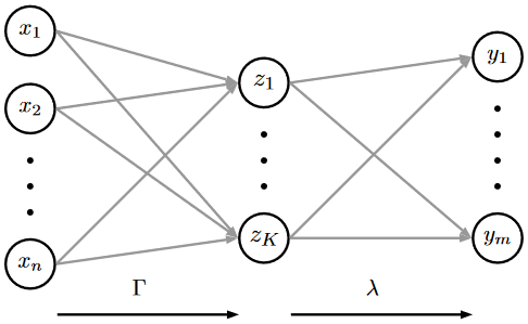
Figure 1 Introduction of intermediate latent states in DBMR for efficient and scalable estimation of Λ.

The task is now to determine the pair of column-stochastic matrices (λ,Γ) from the observation data XY, as given in Eq. (3). Again, we wish to solve the problem with a maximum likelihood approach, which would require solving Eq. (5) by replacing Λ_ij by (λΓ)_ij and the constraints by requiring λ and Γ to be stochastic matrices. This, however, is a computationally hard optimization problem, which in Gerber and Horenko (2017) relaxes to

$$\begin{array}{}\text{(9)}& \left({\mathit{\lambda }}^{*},{\mathbf{\Gamma }}^{*}\right)=\arg \underset{\mathit{\lambda },\mathrm{\Gamma }}{max}\sum _{i=\mathrm{1}}^m\sum _{j=\mathrm{1}}^n\sum _{k=\mathrm{1}}^K{N}_{ij}{\mathrm{\Gamma }}_{kj}\log \left\{{\mathit{\lambda }}_{ik}\right\}\end{array}$$

subject to

$$\begin{array}{}\text{(10)}& {\mathit{\lambda }}_{ik}\ge \mathrm{0},\sum _{i=\mathrm{1}}^m{\mathit{\lambda }}_{ik}=\mathrm{1},{\mathrm{\Gamma }}_{kj}\ge \mathrm{0},\sum _{k=\mathrm{1}}^K{\mathrm{\Gamma }}_{kj}=\mathrm{1}.\end{array}$$

While Eq. (9) produces suboptimal estimates, its advantage comes from the fact that it is concave in both variables λ and Γ, respectively, allowing for a very simple alternating maximization as the optimization procedure (see Gerber and Horenko, 2017). The resulting algorithm is DBMR. Moreover, the method yields ${\mathrm{\Gamma }}_{kj}^{*}\in \mathit{\{}\mathrm{0},\mathrm{1}\mathit{\}}$; i.e., the original input categories are assigned to the reduced system's (latent) categories in a deterministic fashion (no “fuzziness” in the affiliations). The binary nature is a property of the optimal solution (see Gerber and Horenko, 2017). Of course, the number K of latent states is not known in advance and has to be chosen judiciously by compromising between “expressiveness” (the likelihood of the model, i.e., the optimal value in Eq. 9) and “effort” (the number of total parameters to be estimated and their statistical error). This can be done comparing multiple DBMR runs with different K.

The obtained models are also less subject to overfitting issues and are more advantageous in terms of the model quality measures (Gerber and Horenko, 2017; Gerber et al., 2018). This is expressed in the variance of the estimated parameter ${\mathit{\lambda }}_{ik}^{*}$, which shows a $K/n$ times smaller uncertainty than Λ_ij (see Gerber and Horenko, 2017, Theorem and Eq. 7). Again, intuitively this advantage of DBMR over the full model (6) can be seen by noting that from the same amount of data DBMR only needs to estimate k(n+m) parameters, while the full model estimates nm parameters.

Let us emphasize that additionally to all the computational advantages of DBMR that allow it to work with large data sets, its conceptual strength is that it combines model estimation and model reduction in one step. The latent states often have a physical meaning – a property that we shall focus on in our application. All computations in Sect. 4 have been conducted with the DBMR implementation; see Gerber (2017).

3 Meteorological data processing

To apply DBMR, a quantization of the input and output processes into categories has to be performed. First, we discuss the choice of meteorological variables and scales in view of the categorical processes. As input we use a variable related to large-scale atmospheric flow, convective available potential energy (CAPE), a measure for the energy an air parcel would gain if lifted to a specific height in the atmosphere.

3.1 Scales, variables, and data preprocessing

CAPE can be seen as a measure for atmospheric stability, first suggested by Weisman and Klemp (1982). It is defined by

$$\begin{array}{}\text{(11)}& \mathrm{CAPE}=g\underset{z_{\mathrm{LFC}}}{\overset{z_{\mathrm{ET}}}{\int }}{\displaystyle \frac{{\mathit{\theta }}_e-\mathit{\theta }}{\mathit{\theta }}}\mathrm{d}z,\end{array}$$

where θ_e is the pseudo-potential temperature of the ascending air parcel, θ is the potential temperature of the surrounding air, and z_LFC is the so-called level of free convection (LFC). The LFC is the height at which the rising air parcel becomes significantly warmer than its environment; z_ET denotes the height, where the rising air parcel has the same temperature as its environment (ET stands for equal temperature). Thus, regarding its definition (11), CAPE becomes large if the temperature difference between the rising air and the environmental air is large (see Bott, 2016, p. 431ff). For positive CAPE, this difference must be positive. CAPE is determined by the layer thickness between the starting and ending points in space (height) and by the integrand in Eq. (11). Boundary conditions can vary. θ can be a function of z; it depends on the difference between the heights and the potential temperature. As an integral, CAPE is a global variable that we consider a representative variable on the larger scale. To capture convective activity, characterized by strong up- and downdrafts, on the smaller scale, we regard the vertical velocity. Parcel theory predicts

$$\begin{array}{}\text{(12)}& \mathrm{CAPE}\sim {\displaystyle \frac{w_{max}^{\mathrm{2}}}{\mathrm{2}}},\end{array}$$

where w_max is the maximum vertical motion in meters per second expected from the release of CAPE in joules per kilogram (see Dutton, 1976). The relation in Eq. (12) is a kinetic description of a potential which does not have to be released to vertical updraft. Moncrieff and Miller (1976) were the first to use the term CAPE. The USAF Air Weather Service (which changed its name to the Air Force Weather Agency in 1997) simply called it positive area (see Blanchard, 1998). Fritsch and Chappell (1980) called it potential buoyant energy (PBE), while variations of this include +BE and net positive buoyant energy. Despite the abundance of names, it now appears that CAPE is the de facto standard terminology. In Kirkpatrick et al. (2009) over 200 convective storm simulations are analyzed to examine the variability in storm vertical velocity and updraft area characteristics as a function of basic environmental parameter CAPE.

For our studies, the COSMO-REA6 reanalysis data set is used (see Bollmeyer et al., 2015). This reanalysis is based on the non-hydrostatic numerical weather prediction model COSMO (COnsortium for Small scale MOdelling) by the German Meteorological Service (Deutscher Wetterdienst, DWD) using a continuous nudging scheme. It has a horizontal resolution of 6 km and 40 vertical layers (see Bollmeyer et al., 2015). Since we focus on smaller scale convective events conditioned on large-scale dynamics in the atmosphere, we consider the summer months July and August in the years 1995 to 2015. The summer months are predestinated for convective events. The months from May to August are possible. We only worked with 2 months in order not to have too much data. For our analysis, the raw data are hourly REA6 data (Polzin, 2022). We first computed CAPE as a REA6 variable and then averaged it for the respective spatial scale to 12 h means. The sample size of the reanalysis data set used in Sect. 2.2 sums up to S=1302 ($\mathrm{2}\times \mathrm{31}\times \mathrm{21}$). Moreover, REA6 data are available for Germany. In order to focus our method we started at the top left with the first quadrant; see Fig. 2. Here we expect the relatively flat surface in the north of Germany to be more homogeneous and different from the pre-alpine southern regions with forced uplifting. The top left quadrant is bounded by [45.2 to 54.7^∘ N, 5.8 to 15.3^∘ E] and shown in Fig. 2. The northwest coordinate is [5.8^∘ E, 54.7^∘ N], and the southeast coordinate is [15.3^∘ E, 45.2^∘ N]. As a vertical layer the 600 hPa surface is considered because here the latent heat release takes place, and the vertical velocity reaches its maximum (see Müller et al., 2020).

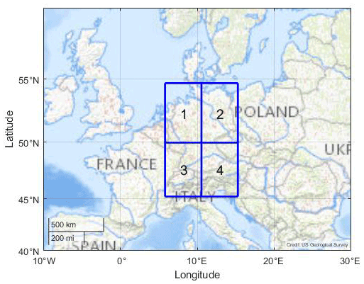
Figure 2 REA6 domain that covers Germany consisting of grid boxes 1 to 4; grid box 1 is applied on the large scale for DBMR and is of approximately 500 km × 500 km. Image credit of the map: US Geological Survey (USGS).

Filtering CAPE and vertical velocity

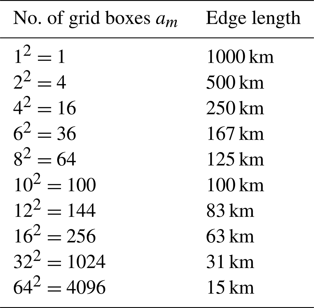
We used the term “domain” for the total region we considered in Fig. 2, “quadrant” for the respective quarters on its large scale, and “grid boxes” for the other partitions of the domain on smaller scales. For the large scale, the domain that covers Germany in Fig. 2 is divided into four 500 km × 500 km quadrants. For smaller scales, the quadrants are refined in a_m grid boxes of different sizes; see Table 1.

Table 1 Number of grid boxes a_m and edge length for box discretization of the atmosphere from the large synoptic scale (1000 km) across intermediate scales up to the meso-γ scale with convective activity (2–20 km).

3.2 CAPE and vertical velocity as in- and output data

According to the meteorological data described in Sect. 3.1, we will set up applicable categories for in- and output. CAPE plays the role of an input variable X as defined in Sect. 2, describing the potential for convection. The spatial arithmetic mean of each of the 500 km × 500 km quadrants is used such that we obtain one CAPE value for each quadrant as the large-scale atmospheric driver. With energy units, CAPE has a nonnegative range of values. The model's output variable Y is vertical velocity, obtained on a smaller scale. Here, Y can take positive and negative values for updrafts and downdrafts, respectively. We average over 250 km × 250 km to 15 km × 15 km according to Table 1.

3.2.1 Categorical input

We consider the range of values for CAPE (X) and generate n categories by $\mathit{\{}x\in X_i\mid b_{i-\mathrm{1}}\le x<b_i\mathit{\}}$. For the category boundaries b_i, we consider the following spaced option in probability using empirical $\mathrm{1}/n$ quantiles as category boundaries b_i. This categorization has the advantage of (almost) equally populated categories. The resulting n categories are denoted by integers $\mathrm{1},\mathrm{\dots },n$. The chosen categorization depends on the amount of available data. We varied input numbers and choose n=10 by subjective physical plausibility. In Sect. 3.1 we set up the meteorological data with a size of the observational data S=1302. That means we have about 130 data points in each CAPE category.

3.2.2 Categorical output

We map vertical velocities ω_i at grid box i on a variable $Y_i\in \mathit{\{}\mathrm{1},\mathrm{2},\mathrm{3}\mathit{\}}$ as

• updraft for Y_i=1, if ω_i≥a₂,

• no draft for Y_i=2, if $a_{\mathrm{1}}\le {\mathit{\omega }}_i<a_{\mathrm{2}}$,

• downdraft for Y_i=3, if ω_i<a₁,

$(a_{\mathrm{1}},a_{\mathrm{2}})\in {\mathbb{R}}^{\mathrm{2}}$ defines a potentially asymmetric interval around zero vertical velocity, which we consider neutral, with a₁<0 and a₂>0. The predefinition of “updraft”, “downdraft”, and “no draft” determines whether there is convection and, if so, how it is directed (upwards or possibly downwards). The choice of (a₁,a₂) depends on the scale of the box over which Y is averaged. In Sect. 4.1 the choice of the interval for our analysis is described. Once this discretization is made, the final output categories needed can be set up. Let Y_i(t) be the discretized vertical velocities at time t with $\mathrm{1}\le i\le a_m$ numbering the grid boxes on the corresponding scale; see Table 1. We define the following categorical process

$$\begin{array}{}\text{(13)}& \widehat{Y}\left(t\right)=\left(\mathit{\#}\left\{Y_i\left(t\right)=\mathrm{1}\right\},\mathit{\#}\left\{Y_i\left(t\right)=\mathrm{2}\right\},\mathit{\#}\left\{Y_i\left(t\right)=\mathrm{3}\right\}\right)\in {\mathbb{N}}^{\mathrm{3}},\end{array}$$

with #{Y_i=k} being the number of grid boxes with vertical velocity mapped onto $k\in \mathit{\{}\mathrm{1},\mathrm{2},\mathrm{3}\mathit{\}}$. Note that ${\sum }_{k=\mathrm{1}}^{\mathrm{3}}\mathit{\#}\mathit{\{}{Y}_i=k\mathit{\}}=m$, the number of grid boxes. There are exactly (a_m+1)² ways to decompose a_m into the (ordered) sum of three nonnegative numbers; thus the number of actually occurring categories $n_{\widehat{Y}}\le (a_m+\mathrm{1}{)}^{\mathrm{2}}$. In DBMR, the numbers of actually occurring categories are counted. These numbers have impact on the probability distribution of the categories for input and output. We try to conclude down- and updraft behavior from the $\widehat{Y}\left(t\right)$, i.e., the distribution of up- and downdrafts. Note that we have no information on the (spatial) structure in this experiment, as the category in Eq. (13) is a triple of numbers for counts of down- and updraft and low vertical velocity.

3.2.3 Interval for vertical draft

The 12 h mean data for day and night serve as a basis for determining the interval for vertical draft which was chosen symmetrically with interval limits $a_{\mathrm{1}}=-\mathrm{0.0048}$ m s⁻¹ and a₂=0.0048 m s⁻¹. In Fig. 3, the histogram of mean vertical velocities for a resolution of 125 km is shown together with the interval that defines the no draft category. For the application of DBMR, the data for day and night are split up and will be applied separately with the same interval for vertical velocity.

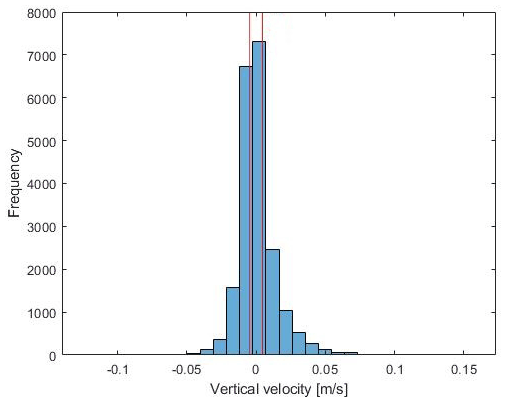
Figure 3 Histogram of spatial mean vertical velocities for day and night for a resolution of 125 km (64 grid boxes on a small scale) is presented. The red vertical lines show the interval for vertical velocity which was selected on the basis of the 75th percentile of the data set. The sample size of the 12 h mean data set for day and night sums up to 2S=2604.

3.3 Reliability and assessment of performance

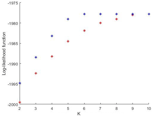
The model reduction is a consequence of using the affiliation matrix Γ, which assigns the n large-scale categories to K<n latent states. In the frame of DBMR we optimize a relaxed log-likelihood; see Eq. (9). We ran DBMR 100 times (with random initializations) for every fixed number K of latent states. For each K, the run with the maximum log-likelihood is presented. We also evaluate the exact log-likelihood, as in Eq. (5), which refers to the case without latent states. Λ in Eq. (5) was replaced by λΓ to compute the likelihood of the reduced model. Figure 4 shows the exact in blue and the relaxed log-likelihood in red, both for the reduced problem, i.e., the one with latent states. The only parameter in the algorithmic procedure introduced above is the reduced process dimension K for the number of latent states. It can be chosen by comparing results for different K and selecting the best reduced model according to one of the standard model selection criteria (cross-validation with a performance criterion, Akaike information criterion (AIC), Bayesian information criterion (BIC), or L-curve approach). For an attempt for model selection, the largest increase in log-likelihood can be found by increasing K=2 to K=3; for K=6, the maximum value has been reached. Note that as n=10, choosing K=10 presents no model reduction. In view of uncertainties and biases for parametrization, vertical velocity can be hard to measure and is likely to be biased in reanalyses. We work with discretize vertical velocity and thus with a less precise variable. This makes the problem of uncertainty and bias less relevant but is definitively not a relief. In a stochastic model for the updraft which is to be developed, one can think of including an additional parameter as a factor to the vertical velocity to allow for tuning with respect to the effect generated by the modeled updraft. Although quantification of model performance is possible here using, e.g., a cross validation study given an adequate score of interest, it is probably not very helpful at this stage. We consider our study rather as a proof of concept ideally preparing grounds for a stochastic model for vertical movement to be inserted into a circulation model. Usefulness should be evaluated then in terms of circulation model simulations. Further work is required to give the latent states a meteorological meaning in the sense of circulation weather types, regarding all seasons separately.

Figure 4 Exact log-likelihood value as in Eq. (5) (blue) and relaxed log-likelihood value as in Eq. (9) (red) of the reduced Bayesian model estimated by DBMR with K latent states for day for a resolution of 125 km (64 grid boxes on a small scale).

4 Reduced model for convective activity

4.1 Dynamics separated by day and night

4.1.1 Affiliation to latent states

In Fig. 5 the box plots show the 12 h averaged CAPE data (spatially averaged over the northwest quadrant of the COSMO-REA6 data) which are assigned to the latent states “high” and “low” on the left and right of each of the two top panels, respectively. The left panel shows the “day” data and the right panel the “night” data. On each box, the central mark indicates the median, and the bottom and top edges of the box indicate the 25th and 75th percentiles of the 10 CAPE categories. The 25th percentiles of the distributions shown for the high latent states overlap the 75th percentiles of distributions shown for the low latent states. The first latent state includes five (for day) and four (at night) CAPE categories with high values. Five (for day) and six (at night) categories are affiliated to the second latent state, which is denoted as low. The structure of the affiliation Γ^* in Eq. (9) is assigned by minimizing information entropy (the likelihood bound). Concerning the question of how the latent states are defined and what criterion the affiliations are based on, we emphasize that the latent states are found by the algorithm itself. During daytime the categories reach values up to 386 J kg⁻¹, whereas at night the values have a range of 343 J kg⁻¹ due to less convective activity; see box plots in Fig. 5. The affiliations to the latent states have no gaps for day and night. That means the latent states are separate from each other. The choice of the spatial scale for the categorical output will influence the latent states identified by the DBMR. The difference between the scales is small (375 km) with 500 km step size on the large scale and 125 km step size on the smaller scale. The scale jump is of factor 4 on the basis of the small scale. The results for three latent states are shown in Appendix A. There is a third latent state which represents mean CAPE categories; see Fig. A1. In the following, the output of the DBMR is discussed.

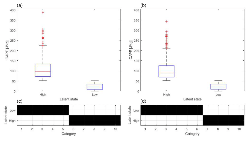
Figure 5 (a, b) Box plots show the 12 h averaged CAPE data which is affiliated to the high and low latent states. Panel (a) presents day data and panel (b) the night data. (c, d) Affiliation of CAPE categories to the latent states. CAPE data are spatially averaged over the northwest quadrant of the COSMO-REA6 data, and the vertical velocity is averaged for a box discretization of 64 grid boxes; see Table 1.

4.1.2 Distributions conditioned on latent states

We discuss probability distributions conditioned on the resulting latent states introduced in Sect. 2.3 in two ways:

• Law[X∣Z] gives the distribution of CAPE X within a latent state Z.

• $\mathrm{Law}[\mathit{\#}\mathrm{1},\mathit{\#}\mathrm{3}\mid Z]$ gives the joint probability distribution of number of grid points with positive and negative vertical velocity. For updraft, #1 denotes #{Y_i=1}, and for downdraft, #3 denotes #{Y_i=3}.

Figure 6 Histograms show probabilities of numbers of updrafts (#1) and downdrafts (#3) conditioned on high (a, b) and low (c, d) latent states. Panels (a) and (c) present day data and panels (b) and (d) the night data. CAPE and vertical velocity data correspond to the data applied in Fig. 5.

The missing number of neutral grid points #{Y_i=2} follows from $\mathit{\#}\mathrm{2}=m-\mathit{\#}\mathrm{1}-\mathit{\#}\mathrm{3}$, with m denoting the total number of grid points. In order to visualize the probabilities of the small scale conditioned on the latent states of the large-scale variable, the entries of the λ matrix in Eq. (9) will be displayed dependent on the number of down- and updrafts. In Fig. 6, K=2 bivariate histograms are shown for day and night respectively. Here the conditional probabilities of matrix λ are displayed for every latent state dependent on the number of up- and downdrafts (#1 and #3). Since the number of smaller scale boxes is a_m, only the lower triangle below the diagonal corresponds to categories. Categories not populated by data are not shown (white). We noticed that in the case that the interval for vertical draft in Sect. 4.1 is increased, fewer data points are in the classifications for the up- and downdrafts (i.e., smaller numbers #1 and #3 change lower triangular probability matrices of Fig. 6). A comparison of different sizes of intervals for vertical draft is not shown here. Increasing the interval makes fewer updrafts and downdrafts, thus moving probability mass away from the diagonal, where large fractions of up-/downdrafts are sitting. In Fig. 6 the results are shown for a 4×4 grid; that means we have 16 grid boxes with vertical velocities. In the histograms the numbers of up- and downdraft range from 0 to 16. Variable Z₁ represents the high latent state and Z₂ the low latent state, as in Fig. 5. The latent states are stochastically disaggregated in probabilities which describe the chance of number of up- and downdrafts conditioned on the high and low latent states. In the top left panel (Z₁, day) of Fig. 6, probability adds up for numbers of updrafts below 10 % to 81 %. In the top right panel, much of the probability mass is allocated to states with no downdraft and little updraft. For $\mathrm{Law}\left[\mathit{\#}\mathrm{1},\mathit{\#}\mathrm{3}\mid Z_{\mathrm{2}}\right]$ in the bottom left panel for the day, high conditional probabilities $\mathbb{P}[\mathit{\#}\mathrm{1},\mathit{\#}\mathrm{3}\mid Z_{\mathrm{2}}]$ concentrate in categories with many boxes with downdraft. Here the probability of numbers of downdrafts of 6 to 16 is 68 %. At night in the latent state Z₂, we observe that a low number of updraft boxes is likely, while the overall up- and downdraft activity seems to be the least probable here (probability concentrating around $(\mathit{\#}\mathrm{1},\mathit{\#}\mathrm{3})\approx (\mathrm{0},\mathrm{0})$). In the bottom left panel (Z₂, night) the probability is accumulated to 82 % for the number of updrafts between 0 and 4.

4.1.3 Output on the smaller scale

Note that the number of possible output categories $\widehat{Y}$ scales quadratically with the number m of grid points considered on the smaller scale. Moving towards the convective scale, m increases, and so does the number of possible output categories; yet the number of data points (1302) stays the same. To avoid the resulting increase of estimation error, we further reduce the number of output categories by dividing the respective numbers for up- and downdraft into three sections, which leaves six categories. We use 15 km × 15 km grid boxes on the convective scale for the output of DBMR. The large scale remains unchanged compared to the previous example. In Fig. 7 the distribution of CAPE in terms of latent states based on kernel density estimation (KDE) is shown. At night, more categories are assigned to the low latent state; the first latent state has a larger mean and median than during daytime.

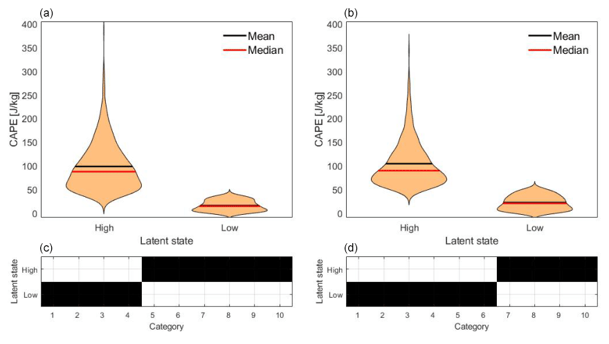
Figure 7 (a, b) Distributions based on kernel density estimation show the 12 h averaged CAPE data which are affiliated to the high and low latent states. Panel (a) presents day data and panel (b) the night data. (c, d) Affiliation of CAPE categories to the latent states. CAPE data are spatially averaged over the northwest quadrant of the COSMO-REA6 data, and the vertical velocity is averaged for a box discretization of 4096 grid boxes; see Table 1.

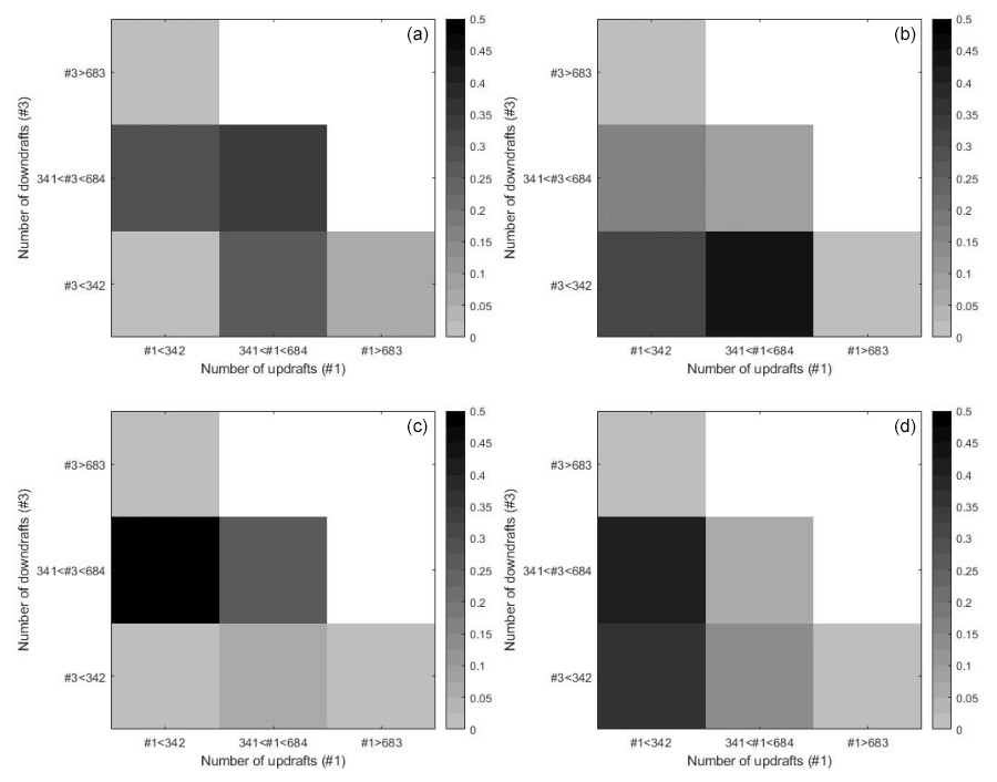
Figure 8 Histograms show probabilities of numbers of updrafts (#1) and downdrafts (#3) conditioned on high (a, b) and low (c, d) latent states. Panels (a) and (c) present day data and panels (b) and (d) the night data. CAPE and vertical velocity data correspond to the data applied in Fig. 7.

In Fig. 8 the conditional probabilities are shown for 1024 boxes of vertical velocities. In the histograms the three sections of numbers of up- and downdraft range from 0 to 1024. The three categories are divided by the following numbers: 0 to 341, 342 to 683, and 684 to 1024 up- and downdrafts. Variable Z₁ again represents the high latent state and Z₂ the low latent state; see Fig. 8. The first latent state is represented in the first row. During daytime, down- or updraft is likely, and during nighttime there is most likely less downdraft than updraft. The smaller scale analysis gives consistent results with the analysis, where the output is on the mesoscale in Fig. 6. There are higher probabilities during daytime for medium to high numbers of up- or downdraft. At night due to less vertical draft, low to medium numbers of up- or downdraft are higher. For the second low latent state, the distributions concentrate on higher and lower numbers of downdrafts and small numbers of updraft.

4.2 Higher number of latent states

The results for three latent states are considered in Appendix A. Figures A1 and A2 show results using CAPE as input with a resolution of 500 km × 500 km on the large scale and a grid of 125 km × 125 km for the output. The scale difference is again of factor 4 according to the first example in Sect. 4.1, where in- and output are on the synoptic scale. Affiliations without gaps lead to a separation of the latent states. “No gaps” means that there is no overlap and a clear separation of the latent states regarding the range of CAPE. This does not apply to every run with DBMR. Here we show the best maximum likelihood bound estimate of 100 runs; see Fig. A1. The affiliations have no gaps for day and night. Again we have more variance of the conditional probabilities during daytime. At night, there is less variance of the conditional probabilities, with a concentration at low numbers of downdraft or updraft boxes. A hierarchy of three different probability configurations arises for updraft, downdraft, and no draft. When the number of latent states K is further increased, the latent states can be clustered in groups of high, low, and medium CAPE categories. In Fig. A1, the top box plots show CAPE categories by three latent states for the daily mean (left – day and right – night), and in the middle the affiliation of CAPE categories to the latent states is presented. For higher K, the number of latent states with affiliation without gaps is higher at night compared to day.

4.3 Implications for general atmospheric dynamics

In Sect. 4.1 we discussed the results of the Bayesian model reduction from a mathematical perspective, and in Sect. 4.2 we interpreted the outcomes for a higher number of latent states. The method groups input categories into fewer latent states. These are interpreted as reduced states for the large-scale atmospheric dynamics with respect to their probabilistic impact on vertical motion. We applied an energetic variable as the driver on the large scale. CAPE is the convective available potential energy. It does not have to be fully available, meaning that high CAPE values do not necessarily lead to convective activity on smaller scales but increase the probability of smaller scale convective activity. The release of kinetic energy of a certain CAPE level to vertical movement needs triggers such as flows over mountains or forests, which lead to instabilities of the hydrostatic equilibrium. The dependence on surface conditions on the earth requires a probabilistic way of thinking. Therefore the mathematical tool DBMR provides a simple probabilistic description. Using the method, we intend to draw conclusions about categorical processes in the atmosphere. Since the system can not be in two different categories simultaneously, categories are disjoint, and the relation between the probability for the large scale and smaller scale can be formulated via the conditional probabilities and the conservation of the total probability. The methodology breaks up probability calculations into distinct parts and relates marginal probabilities to conditional probabilities. The aim of this work is to test the stochastic method in an meteorological application towards a reduced categorical model of smaller scale convective activity in the atmosphere depending on large-scale drivers.

To analyze the relation of large-scale dynamics in the atmosphere to smaller scale categorical processes, the COSMO-REA6 reanalysis data set was applied (see Bollmeyer et al., 2015). We averaged CAPE for 500 km × 500 km and the vertical up- and downdrafts in 125 km × 125 km domains, as described in Sect. 3.2. Regarding the summer months July and August in the years 1995 to 2015, CAPE reaches averaged values between 0 and 400 J kg⁻¹, and the vertical velocities have ranges from −0.15 to 0.2 m s⁻¹ on the mesoscale and −1.7 to 1 m s⁻¹ on the convective scale. In the meteorological setting we showed how the Bayesian model reduction is performed. We combined large-scale CAPE with a subgrid mesoscale time series for vertical velocity and count the numbers of up- and downdrafts. Therefore we mapped vertical velocities as updraft, no draft, and downdraft dependent on an interval around zero vertical velocity. In the preprocessing of Sect. 4.1, we adjusted the interval for vertical draft with a range of 0.0096 m s⁻¹ according to the meteorological data. The interval was chosen symmetrically on the basis of the histogram of mean vertical velocities in Fig. 3. We chose a number of 10 input categories and reduced these to two latent states. This was done for day and night, respectively.

In Fig. 5 the summary statistics with the affiliation of input categories to the latent states are presented. The affiliations in Figs. 5 and 7 have no gaps, meaning that the affiliations are interrelated and are not interrupted. The affiliations lead to a separation of the latent states in the box plots for day and night. Thus a certain range of CAPE values can be assigned to every latent state. During daytime the range of values for the high latent state is at around 400 J kg⁻¹ and greater compared to the corresponding latent state during nighttime. For smaller scales we reduced the number of output categories. In Fig. 7 at the bottom, six high and four low CAPE categories for the daily mean and four high and six low CAPE categories at night are affiliated. As a result of the averaging, the categories are almost evenly distributed over the latent states. The convective activity of the atmosphere is stronger during the day than during nighttime. Therefore, the vertical draft is less at night than during the day. Mean and median are around 100 J kg⁻¹ for the high latent state and 25 J kg⁻¹ for the low latent state. The mean and median are similar for day and night. There is a difference for the variance. At night the distribution of the high latent state is sharper due to less variance; only four categories are affiliated compared to the daily mean.

Joint probability distribution of the number of grid points with positive and negative vertical velocity conditioned on the resulting latent states is shown in Figs. 6 and 8. The sum of the probabilities of all categories for every box is 1. Increasing the interval for vertical draft makes fewer up-/downdrafts, thus moving probability mass away from the diagonal, where large fractions of up-/downdrafts are sitting. There are higher probabilities during daytime for medium to high numbers of up- or downdraft. Lots of updrafts during daytime lead to the existence of a lot of downdrafts due to mass conservation. At night due to less vertical draft, low to medium numbers of up- or downdraft are higher. For the low latent state, the distributions in Figs. 6 and 8 are concentrated on higher and lower numbers of downdrafts and small numbers of updraft. The representation of probabilities of numbers of updrafts and downdrafts conditioned on the latent states in Fig. 8 corresponds to the results on the mesoscale in Fig. 6. The generation of kinetic energy of a certain CAPE level to vertical draft on smaller scales can occur up to a few hours later. A temporal shift for the in- and output could have an effect on the stochastic relation shown in Fig. 6. We consider the 12 h means. For data with a higher temporal resolution, one could realize a shift of 2–4 h for the input. This is deferred to future studies.

5 Conclusions

It is of importance to identify stochastic models using categorical approaches compared to fluid mechanics described by continuous partial differential equations. In this study, a recent algorithmic framework called Direct Bayesian Model Reduction (DBMR) is applied which provides a scalable probability-preserving identification of reduced models directly from data (see Gerber and Horenko, 2017). We assume that the output of a Bayesian model depends on the input through a latent variable, which can merely take a small number of different latent states. In this work, a direct Bayesian model reduction of smaller scale convective activity conditioned on large-scale dynamics is investigated with regard to intermediate latent states. We combined the convective available potential energy (CAPE) as a large-scale flow variable with smaller scale subgrid time series for vertical velocity. Therefore we mapped vertical velocities as updraft, no draft, and downdraft dependent on an interval around zero vertical velocity and count the numbers of up- and downdrafts. Data sets of daily means of 12 h for day and night were computed using COSMO-REA6 reanalysis over a domain that covers Germany for a period of the summer months July and August in the years 1995 to 2015. In the analysis the scales from 500 to 125 km (mesoscale) and up to 15 km were considered. The categorical data analysis was done for day and night and discussed for different numbers of latent states. We chose a number of 10 input categories and reduced these to two and three latent states.

The step from the fluid continuum described by partial differential equations to a categorical stochastic description with DBMR provides a reduced model defined on a set of a few latent variables. These are interpreted as reduced states for the large-scale atmospheric dynamics with respect to their probabilistic impact on vertical motion. For two latent states the input is separated into categories with high and low CAPE values, whereas for three latent states, we have an affiliation to categories with high, medium, and low CAPE values. The output categories for the vertical velocity describe the number of up- and downdrafts. In the result, we gain conditional distributions for the numbers of up- and downdrafts conditioned on the latent states for day and night. In the application we found a probabilistic relation of CAPE and vertical up- and downdraft.

For a resolution of 125 km we applied a 4×4 grid and had 16 boxes with vertical velocities. During daytime the chance for updraft is higher conditioned on the latent state with high CAPE values. Probability adds up for numbers of up- or downdrafts higher than 10 % to 81 %. The distribution for the latent state with low CAPE values has higher probabilities at high numbers of downdrafts. Here the probability of numbers of downdrafts of 6 to 16 is 68 %. At night probability adds up at small numbers of downdrafts for the latent state with high CAPE values. For low CAPE values, we observe that a low number of updrafts is likely. The probability is accumulated to 82 % for the number of updrafts between 0 and 4.

On the smaller scale, with a resolution of 15 km, we applied a 32×32 grid and had 1024 boxes with vertical velocities. We divided the output into three categories of low (0 to 341), medium (342 to 683), and high (84 to 1024) numbers of up- and downdrafts. During daytime, the probability for a medium number of up- and downdrafts is 34 % for the latent state with high CAPE values. Here low and high numbers of up- and downdraft have a small probability. For low CAPE values, the maximum in the distribution occurs for a medium number of downdrafts and low number of updrafts at 50 %. At night the probability adds up at low to medium numbers of downdrafts for the latent state with high CAPE values, and for low CAPE values, we observe that the chance of low and medium numbers of updrafts is 82 %. The distribution for the smaller scale resolution (15 km) is a stochastic aggregation of the distribution with a resolution of 125 km. Therefore the distributions are qualitatively similar. When the number of latent states is further increased, the latent states can be clustered into groups of high, low, and medium CAPE categories.

The model reduction of smaller scale convective activity is part of a development process for a model with a stochastic component for a conceptual description of convection embedded in a deterministic atmospheric flow model. Various energetic variables are applicable on the large scale. A potential driver to control small-scale models is the Dynamic State Index (DSI) in Müller et al. (2020) and Müller and Névir (2019), an “adiabaticity indicator”. Other large-scale variables driving the smaller scale stochastics are the available moisture or vertical wind shear. The presented approach provides a basis for further research on smaller scale convective activity conditioned on other possible large-scale drivers.

Appendix A

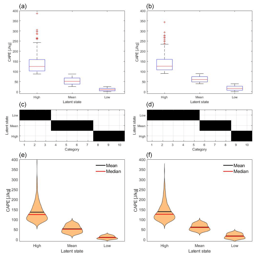
Figure A1 Box plots show the 12 h averaged CAPE data which are affiliated to the high, mean, and low latent states. Panel (a) presents day data and panel (b) the night data. (c, d) Affiliation of CAPE categories to the latent states. (e, f) Distribution of CAPE in terms of latent states based on kernel density estimation. CAPE data are spatially averaged over the northwest quadrant of the COSMO-REA6 data, and the vertical velocity is averaged for a box discretization of 64 grid boxes; see Table 1.

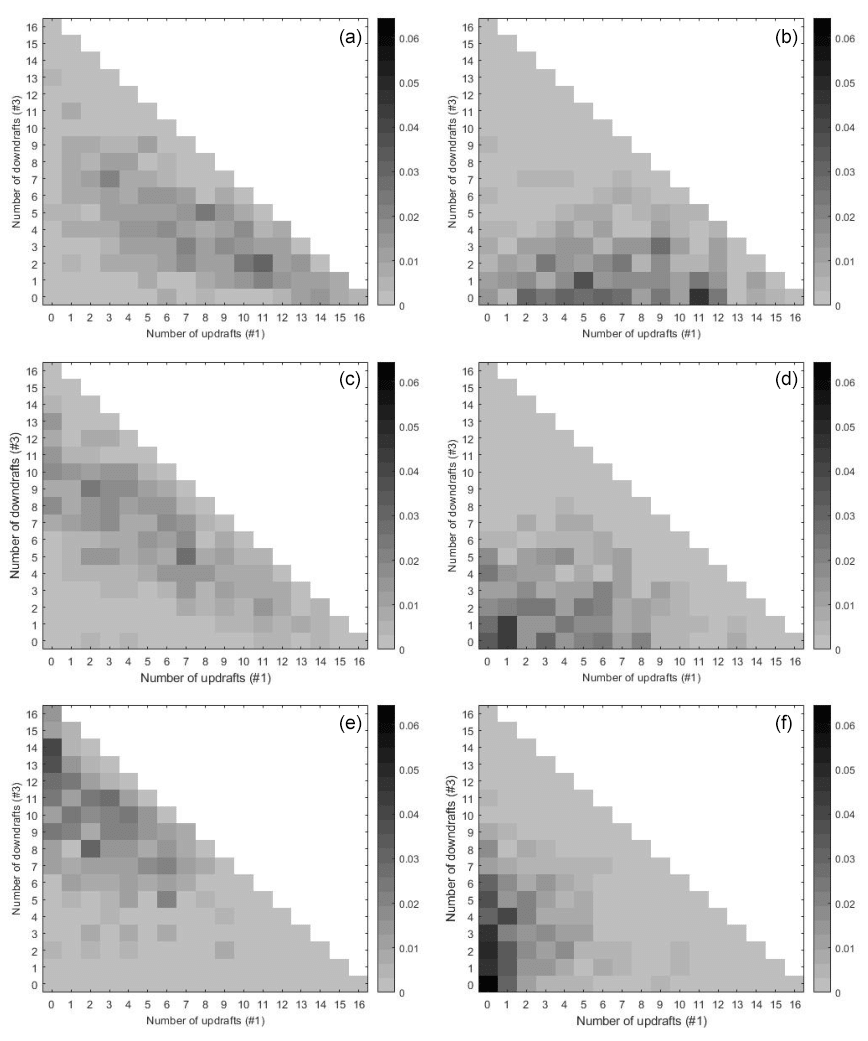
Figure A2 Histograms show probabilities of numbers of updrafts (#1) and downdrafts (#3) conditioned on high (a, b), median (c, d), and low (e, f) latent states. Panels (a), (c), and (e) present day data and panels (b), (d), and (f) the night data. CAPE and vertical velocity data correspond to the data applied in Fig. A1.