the Creative Commons Attribution 4.0 License.
the Creative Commons Attribution 4.0 License.
 | 06 Oct 2022
Using a hybrid optimal interpolation–ensemble Kalman filter for the Canadian Precipitation Analysis
Dikraa Khedhaouiria
Stéphane Bélair
Vincent Fortin
Guy Roy
Franck Lespinas
Several data assimilation (DA) approaches exist to generate consistent and continuous precipitation fields valuable for hydrometeorological applications and land data assimilation. Usually, DA is based on either static or dynamic approaches. Static methods rely on deterministic forecasts to estimate background error covariance matrices, whereas dynamic approaches use ensemble forecasts. Associating the two methods is known as hybrid DA, and it has proven beneficial for different applications as it combines the advantages of both approaches. The present study intends to explore hybrid DA for the 6 h Canadian Precipitation Analysis (CaPA). Based on optimal interpolation (OI), CaPA blends forecasts and observations from surface stations and ground-based radar datasets to provide precipitation fields over the North American domain. The application of hybrid DA to CaPA consisted of finding the optimal linear combination between (i) an OI based on the Regional Deterministic Prediction System (RDPS) and (ii) an ensemble Kalman filter (EnKF) based on the 20-member Regional Ensemble Prediction System (REPS). The results confirmed the known effectiveness of the hybrid approach when low-density observation networks are assimilated. Indeed, the experiments conducted for the summer without radar datasets and for the winter (characterized by very few observations in CaPA) showed that attributing a relatively high weight to the EnKF (50 % and 70 % for summer and winter, respectively) resulted in better analysis skill and a reduction in false alarms compared with the OI method. A deterioration in the moderate- to high-intensity precipitation bias was, however, observed during summer. Reducing the weight attributed to the EnKF to 30 % alleviated the bias deterioration while improving skill compared with the OI-based CaPA.
- Article
(4144 KB) - Full-text XML
- BibTeX
- EndNote


Errors inherent in the observed data, the parameterization of subgrid processes, the initial conditions, and the model physics, to name a few, combined with the chaotic nature of the atmosphere (Lorenz, 1963), lead to uncertain numerical weather prediction (NWP) forecasts, especially for precipitation fields (Ebert, 2001). Today, most meteorological centers have developed their operational ensemble prediction systems (EPSs) to consider these uncertainties (Buizza, 2019). EPSs provide, for the same time and location, a set of forecasts obtained by introducing perturbations at different modeling stages (e.g., initial and boundary conditions; Buizza, 2019).
EPSs deliver probabilistic meteorological information that is also valuable for data assimilation (DA) systems, which will be the focus of this paper for the particular case of the Canadian Precipitation Analysis (CaPA; Mahfouf et al., 2007; Fortin et al., 2015). The CaPA system produces gridded precipitation fields based on NWP forecasts adjusted with observed precipitation (ground stations and radars) using optimal interpolation (OI) assimilation methods (Fortin et al., 2015; Lespinas et al., 2015; Fortin et al., 2018). Using EPSs in CaPA would allow the estimate of the “errors of the day” from short-term ensemble forecasts via the computation of flow-dependent background error covariances (Kalnay et al., 2007). As opposed to a static assimilation approach, weights attributed to the background and the observations would be potentially better distributed (Wang et al., 2007). However, DA systems using EPSs such as ensemble Kalman filter (EnKF; Evensen, 2003) often require large ensembles to avoid sampling errors and the associated rank problem of covariance matrices (Houtekamer and Zhang, 2016). In contrast, DA systems using deterministic forecasts such as standard variational approaches are more computationally efficient (Wang et al., 2008a; Houtekamer and Mitchell, 1998). Nevertheless, these DA methods use assumptions on the homogeneity, the isotropy, and the invariance of error covariance matrices. To combine the desirable aspects of both DA scheme families (Houtekamer and Zhang, 2016), linear combinations of the static and the dynamic error covariance matrices, known as hybrid approaches, have been developed (Hamill and Snyder, 2000; Wang et al., 2008a; Kleist and Ide, 2015).
Hybrid assimilation schemes have been thoroughly and successfully tested for many applications. Hamill and Snyder (2000) combined the three-dimensional variational (3DVar) and EnKF DA schemes for atmospheric assimilation for the United States of America (USA) domain. The authors showed improvements over 3DVar alone, especially in data-poor networks and, to a lesser extent, in denser networks. For the same domain, Wang et al. (2008a) also showed that analyses generated with the same hybrid approach (3DVar–EnKF) produced 12 h forecasts that were more accurate than 3DVar and confirmed the efficiency of the method in regions with low observation density. Other studies worked on different hybridization variants; for example, Wang et al. (2008b) combined the ensemble transform Kalman filter (ETKF) and 3DVar for the DA system over the USA using the Weather Research and Forecasting (WRF) model. The authors drew the same conclusions regarding the density of observations. In ocean forecasting, Counillon et al. (2009) combined optimal interpolation (OI) and an EnKF method. They demonstrated a reduction in forecast errors using hybrid covariances for small dynamic ensembles (10 members) relative to OI or EnKF.
The successful combination of two different DA schemes in order to produce better analysis and forecasts has led various meteorological centers to use this approach for operational products, such as Houtekamer et al. (2019) for the Canadian Centre for Meteorological and Environmental Prediction (CCMEP) of Environment and Climate Change Canada (ECCC), Bonavita et al. (2015) for the European Centre for Medium-Range Weather Forecasts (ECMWF), and Penny et al. (2015) for ocean forecasting at the National Centers for Environmental Prediction (NCEP). Several other studies have shown the relevance of hybrid approaches for DA, but a full review of their uses is beyond this research scope.
At CCMEP, the availability of the Regional Ensemble Precipitation System (REPS) encompassing the North American domain allows the investigation of hybrid approaches for analyses at a higher resolution than those currently existing (see Houtekamer et al., 2019, for the global domain with its horizontal grid spacing of about 39 km). The 20-member REPS product is available at an approximately 10 km grid spacing and has been operational since summer 2019. The purpose of this study is to explore the potential improvements brought by hybrid approaches to the operational 6 h CaPA, which is solely based on an OI where the background field is the Regional Deterministic Prediction System (RDPS; Caron et al., 2015). Various factors motivated the exploration of the well-established and well-documented hybrid DA methods. First of all, the REPS is fully operational and has the same domain and resolution as CaPA; therefore, it can be used as a background field without any interpolation. Second, the hybrid approaches may positively impact the several data-poor areas (e.g., northern Canada) of the CaPA domain where OI has its limitations. Third, to our knowledge, no other studies have explored this approach for precipitation analyses. Finally, the specificity of OI in CaPA makes it interesting to explore in the context of hybrid DA approaches. Indeed, conclusions from several studies on hybrid DA methods have been generally obtained when combining static and dynamic DA approaches (Wang et al., 2007; Counillon et al., 2009). However, OI in CaPA is not, strictly speaking, static as observations, and forecasting errors are updated for each analysis time using variographic analysis (Fortin et al., 2015) as opposed to static errors estimated with the climatology.
The rest of the article is organized as follows: Sects. 2 and 3 introduce the datasets and the hybrid analysis scheme methodology, respectively; Sect. 4 describes the method to select the optimal weighting for the hybrid approach; Sect. 5 presents the experimental design; the verification strategy is given in Sect. 6; the results of the experiments are made available in Sect. 7; and the conclusion is given in Sect. 8.
2.1 Model description
The operational 20-member Regional Ensemble Precipitation System (REPS, version 3.0.0; ECCC, 2019) and the Regional Deterministic Prediction System (RDPS; Caron et al., 2015) use the same configuration. The domain covers the North American continent (Fig. 1) with a horizontal grid spacing of 0.09∘ (∼10 km) and 84 vertical levels. The RDPS and REPS generate 72 h forecasts four times per day – at 00:00, 06:00, 12:00, and 18:00 UTC. Uncertainty in the REPS is represented by perturbed initial conditions (ICs) and lateral boundary conditions (LBCs) and stochastically perturbed physics tendencies (SPPTs; Charron et al., 2010) but with the same physical parameterization for all members. The atmospheric ICs derive from a 20-member interpolated Global Ensemble Prediction System (GEPS; Charron et al., 2010; Houtekamer et al., 2014) analysis perturbation centered around the RDPS initial analysis. Every hour, the LBCs are also provided by the GEPS.
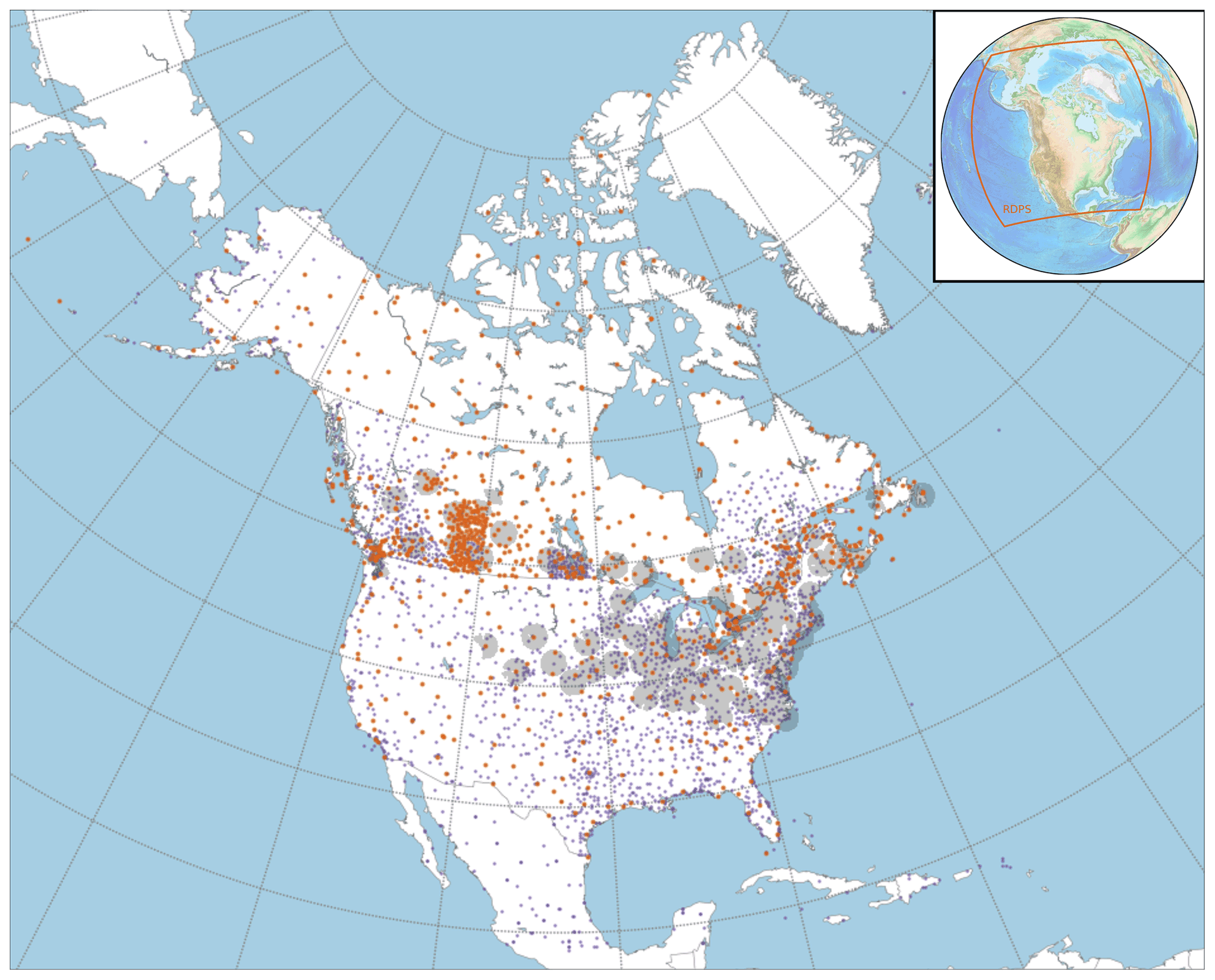
Figure 1Blue and orange dots represent the various precipitation networks and the surface synoptic observation (SYNOP) stations assimilated in summer 2019, respectively. Shaded gray areas denote the assimilated portion of radar beams. The inset illustrates the analysis domain.
2.2 Observations
The 6 h analysis assimilates precipitation from surface stations from Canadian networks and networks in the contiguous United States (CONUS), some of which are operational only during the warm season. A total of 33 and 31 C-band radar quantitative precipitation estimates (QPEs), covering the US and Canada (mostly located along the USA border), respectively, are also assimilated. Since 2017, new Canadian dual-polarization Doppler radars have been progressively replacing their C-band counterparts. They contribute to retrieving information on a broader range of meteorological events than standard C-band radars (Kollias et al., 2020) and would ultimately enable better analysis. Both types of observation follow an extensive quality control, as described in Sect. 3.2.
2.3 Stage IV precipitation
In addition to verification at station locations (see Sect. 6.1), the 6 h analyses were also compared to 6 h Stage IV (ST4) analysis from the National Centers for Environmental Prediction (NCEP; Lin and Mitchell, 2005). The objective is to allow verification against spatially continuous precipitation fields. ST4 is a mosaic of regional multi-sensor (gauges and WSR-88D radars) analysis that is designed differently from CaPA and ensures a certain degree of independence during the verification. The ST4 domain covers the CONUS; however, due to known limitations in the western domain (see Nelson et al., 2016, for more details), only the CONUS east of 105∘ W was used for verification purposes. The ST4 native horizontal spacing of ∼4.7 km was interpolated to the coarser RDPS grid using circular filtering (see Fig. 3a in Jacques et al., 2018) to allow for verification on a common grid. ST4 will not provide a picture of performance over the entire RDPS domain, as Canada and the southern part of the RDPS are not covered. However, ST4 is a valuable dataset that could help compare the results obtained with the different configurations of the hybrid approach.
3.1 Hybrid assimilation approach for the precipitation analysis
Similarly to what was proposed by Hamill and Snyder (2000), the background field error covariance matrix using the hybrid approach () is a weighted sum of the OI-based (PbOI) and dynamically based (Pbd) matrices:
where the parameter β is comprised between 0 and 1, ensuring that the total background error covariances are conserved (Wang et al., 2008a). Thus, when β=0, the analysis is solely based on the OI, whereas the background errors are ruled by the REPS when β=1. The β selection methodology is further detailed in Sect. 4.
It is worth mentioning that the precipitation from both the observation and background model (y) are primarily Box–Cox transformed such that
where in the CaPA configuration. This preprocessing strategy has been used because it provided more skillful analyses (Fortin et al., 2015; Lespinas et al., 2015). The final analyses are obtained from the back-transformation, followed by corrections of the biases induced by this transformation (Evans, 2013).
An exponential and isotropic model is assumed for the spatial correlation function of the background field errors (Fortin et al., 2015). The ith row and jth column of PbOI writes as follows:
where , δ(i,j), and lOI are the variance of the background errors, the Euclidean distance between locations i and j, and the correlation length, respectively. In the CaPA algorithm, parameters , lOI, and (where the latter is the variance errors of the observation), which are needed to build the observation error covariance matrix (explained further below), are estimated before the analysis as such using a variographic analysis of the innovations. The innovations are classically defined as , where d, xf, and H correspond to the measurements, the forecasts, and the observation operator (which is here the nearest-neighbor interpolation), respectively (Fortin et al., 2015).
The degree of spatial dependence of the innovations is described through a theoretical exponential function fitted on the empirical semivariogram (Cressie, 2015) and is defined as
Here, zi and zj correspond to the innovations at locations i and j, respectively, and corresponds to the variance errors of the observation. As opposed to other DA approaches where the error matrix is static, the variographic analysis is computed for each analysis time step and, therefore, allows for time varying elements in .
The covariance matrix Pbd depicts the flow-dependent errors estimated from the REPS and is defined as
where denotes the anomalies estimated from the N-member ensemble at m grid points. The superscript T corresponds to a matrix transpose. To avoid underestimation of the variance of the background errors due to the limited size of the dynamic ensemble (Houtekamer and Mitchell, 1998), the anomaly computation follows the suggestions of Hamill and Snyder (2000) and writes as follows:
where the subscript refers to the jth column of a given matrix, and Xf is the (m×N) precipitation ensemble forecast matrix. The m length vector corresponds to the average across the N members without the jth member.
The analysis is performed sequentially for each grid cell, for which the error matrices are estimated using up to 16 neighbors per observation type to speed up the computation (Fortin et al., 2015). Therefore, when assimilating both surface observations and radar QPEs, is a matrix of size up to 32×32. In cases where no observation is encountered within a radius of 500 km, the analysis process is accelerated by setting the grid-cell value equal to the background field.
The equations for the analysis estimates are solved as follows:
Here, R and W are the observation error covariance matrix (see details in Fortin et al., 2015) and the weight vector, respectively.
The variances of the error made by estimating the precipitation analysis are obtained from the covariance structure and the weights as follows (Fortin et al., 2015):
For the hybrid approach, the variance of background errors is defined as
where is estimated with the variogram modeling presented in Eq. (4). In contrast, has the advantage of being directly estimated from the REPS and is defined for a given grid-cell location, so, as follows:
where is the N-length vector of REPS precipitation at location so, and is the ensemble mean at the same location, as defined in Eq. (5).
In addition to the estimate of the analysis error already provided by the OI, CaPA provides a spatially and temporally varying index that describes the confidence granted to the precipitation analysis. This index is based on the assumption that the most reliable data is observation. For a given grid cell and valid time, the confidence index of the analysis (CFIA) has been defined as 1 minus the ratio of the error variances of the analysis () to the background ():
The CFIA ranges from 0 to 1. CFIA values close to 1 (0) depict high contributions of the observation (background) to the analysis estimates. CFIA values close to 0 occur when no observations are assimilated in the vicinity of a given grid cell. Thus, this index is convenient for users desiring to select only grid cells influenced by observations. Using the hybrid approach in CaPA enables one to account for flow-dependent errors. It would, therefore, have impacts on CFIA estimates, as discussed further in Sect. 7.4.
3.2 Quality control of the observations during the assimilation
Observed surface precipitation and radar QPEs undergo an extensive quality control (QC) process to remove untrustworthy data. The QC is automatically done for each assimilation valid time, leading to a time-varying number of assimilated observations, as described in Lespinas et al. (2015) for surface observations and in Fortin et al. (2015) for radar QPEs. A temporal QC is performed to identify persistent problems that occur over a given period, such as a station that reports no or too much precipitation over a long time period. Rejecting or keeping a surface station is based on the statistical distribution of the differences between the observation and the analysis obtained over the most recent cases (see details in Sect. 2b in Lespinas et al., 2015). A different quality control, hereafter referred to as spatial QC, is carried out to identify surface stations that have very different precipitation than those in their immediate vicinity. For this purpose, an analysis is estimated at a site sk () using neighboring stations in a leave-one-out (LOO) approach. The observation at the same site () is rejected or is deemed invalid if the following is not fulfilled:
where tol is a tolerance factor set equal to 4 for the operational CaPA. Both the observed precipitation and analysis estimates of Eq. (12) underwent a Box–Cox transformation beforehand (see Eq. 2). The size of the neighborhood depends on the background field correlation length, which varies for each analysis and, therefore, adapts with seasons (Lespinas et al., 2015). This approach helps avoid the rejection of very localized summer precipitation events. An additional QC is also applied during the cold season, with the rejection of radar QPEs and surface observations associated with windy condition (Rasmussen et al., 2012). Several other QC measures are applied to precipitation input datasets, but their extensive description is beyond the scope of this paper (see Fortin et al., 2015, and Lespinas et al., 2015, for further information). Figure 1 illustrates the stations and radars that passed the QC for summer.
In CaPA, hybrid DA approaches can impact the QC of observations. Indeed, changing the past analysis values (used in the temporal QC) and the standard deviation of the analysis error (used in the spatial QC) can induce differences in the number of assimilated stations. The results showed slight changes in the number of observations assimilated when using hybrid approaches and are, therefore, not detailed in this study.
Analysis experiments using with a 0.1 step are conducted for each valid time to identify the β value that provides the most accurate precipitation analysis. At least two different options are possible to select the most suitable β. First, the analyses are conducted for a given season, and the β that minimizes an objective function is selected and stored for future use. The second option consists of choosing the most suitable β for each valid time, implying a dynamic selection of β. While the first option is computationally inexpensive, as β values are estimated once for each season, it suggests that this parameter remains constant over years. The second option is more flexible but requires data independent of those used during the precipitation verification step, which is required to evaluate the CaPA system (Sect. 6).
To understand the choice that has been made for either option, the CaPA configuration must be presented first. CaPA generates two types of precipitation analysis. The first is conducted only at surface station locations in a leave-one-out framework (hereafter, CaPA-LOO). This computationally inexpensive analysis is both a QC step to reject suspicious precipitation observations (see Sect. 2b in Lespinas et al., 2015, and Sect. 2.2 below) and a valuable dataset for verification purposes in a cross-validation manner. The second type of analysis is performed for each grid cell of the domain.
A dynamic selection of β for each analysis valid time would have been the preferred option, as it would not have required manual updates during, for example, major operational upgrades of the different systems (CaPA, REPS, or RDPS). For this purpose, preliminary tests using random samplings of the CaPA-LOO datasets have been done. For each valid time, a training sample was employed for the β selection, while the testing sample was kept for objective verification. The training and the testing sample sizes had to be large enough to capture the optimal β value over the domain and to realize consistent precipitation verification, respectively. Different sample sizes were tested with up to 40 % of the initial CaPA-LOO dataset to estimate the optimal β. However, the results were too noisy due to sampling effects, especially during winter when the station density is relatively low. For this reason, the first option to select the β value was preferred. The normalized root-mean-square error (NRMSE) averaged over a selected period and based on the CaPA-LOO datasets was chosen to identify the optimal β. The normalization was realized to lessen the influence of the total precipitation amount during a given analysis time step (Bachmann et al., 2019). For more reliability, the NRMSE is computed only at surface synoptic observation (hereafter SYNOP) stations and manual SYNOP stations during the summer and the winter, respectively, and is defined as follows:
where M, aLOO, and o correspond to the number of cases during a given valid time, the LOO analysis, and the observations, respectively. The NRMSE values of zero (0) illustrate perfect analyses.
Two sets of 2-month experiments were conducted: (i) one over July to August 2019 (hereafter summer) and (ii) one over January to February 2020 (hereafter winter). For each 6 h valid time, 11 sets of analyses were produced with the different β values presented in Sect. 4.
Summer and winter experiments are expected to differ due to both the background model's distinct seasonal performance with respect to representing precipitation and the significantly smaller assimilated datasets in winter. The usefulness of a hybrid configuration has been demonstrated when low-density observation networks are assimilated (Hamill and Snyder, 2000; Wang et al., 2008a, b). Thus, to verify this point without being strongly influenced by seasonal effects, an additional experiment was conducted without the assimilation of radar QPEs. The experiment without radar was only conducted during the summer as no impact is expected during the cold season, during which radar QPEs are not assimilated.
6.1 Comparisons against observations from surface stations
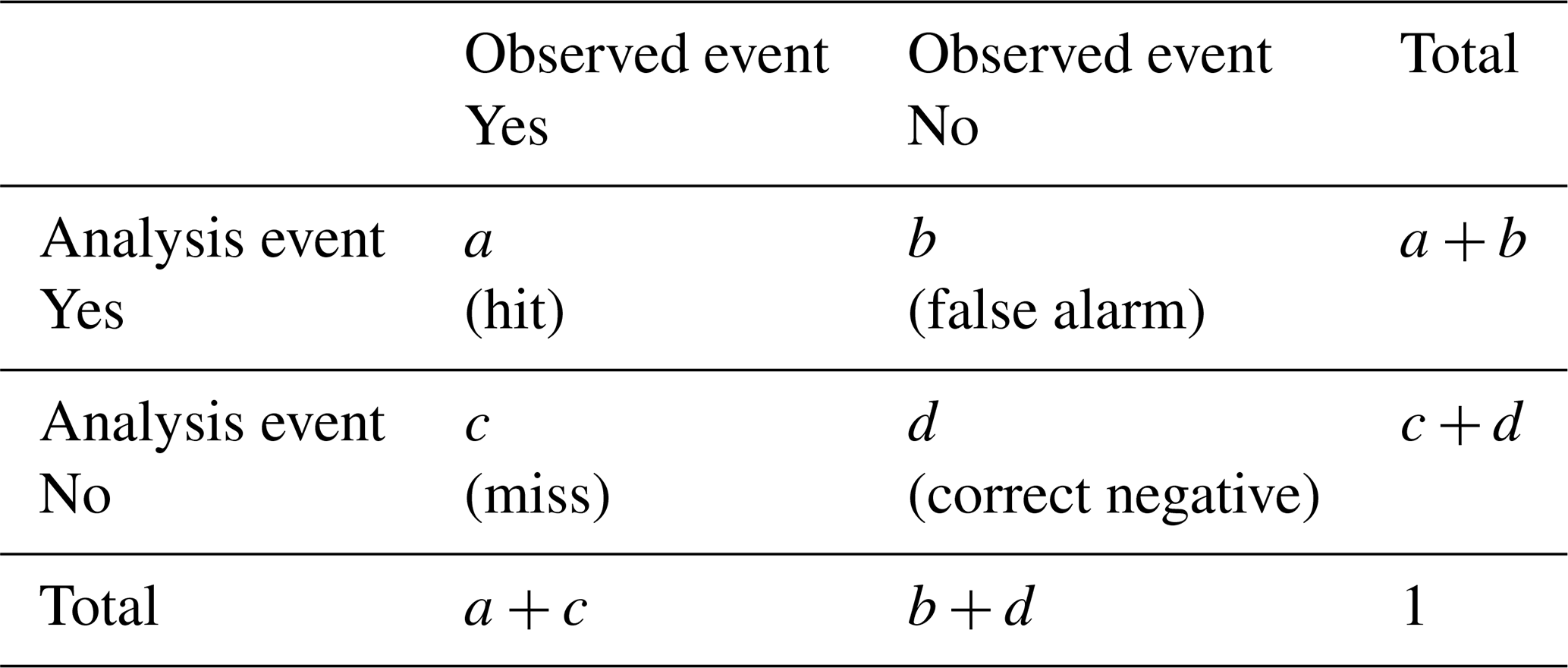
Based on the 2×2 contingency table for binary events (Table 1), four different metrics, commonly used for precipitation objective evaluation, are computed for the different configurations of the LOO analysis. The first is the frequency bias index (FBI), which compares the frequency of events in the analyses to those in the observations. The second is the equitable threat score (ETS), which assess the agreement between the analysis and the observations. Following the annotations in Table 1, the FBI and ETS are expressed as follows:
where illustrates the hits expected by chance and makes the ETS less sensitive to the climatological frequency of precipitation events. The probability of detection (POD) and the false alarm ratio (FAR) are the other two metrics and are defined as follows:
The FBI-1 – which is equivalent to the normalized difference between false alarms and missed events – is preferred in the following, as positive (negative) values imply positive (negative) bias (Lespinas et al., 2015). FBI-1 and FAR values of zero (0) are optimal, while ideal POD and ETS values are one (1). For the four metrics, binary events are defined as 6 h accumulations meeting or exceeding selected thresholds, here 0.2, 1.0, 5.0, and 10.0 mm. Higher thresholds are not shown because the samples were too small, leading to overly noisy scores.
Table 1The 2×2 contingency table for binary events, where a, b, c, and d correspond to the frequency of hits, false alarm, misses, and correct negatives, respectively.
Statistical differences between the scores using β=0.0 (hereafter the reference experiment) and β>0.0 were assessed using stationary block bootstrapping with a 95 % confidence level (Brown et al., 2012). The bootstrapping implementation specific to CaPA is detailed in Lespinas et al. (2015).

Figure 2The NRMSE averaged over the summer period without (a) and with (b) the assimilation of radar QPEs and over the winter (c) for the different β values.
6.2 Comparisons against Stage IV
Two different types of comparison against ST4 were conducted. First, aggregated areal coverages of 6 h accumulated precipitation meeting or exceeding selected accumulation thresholds were assessed to evaluate how precipitation is distributed in ST4 and CaPA.
Second, the fraction skill score (FSS) was computed to assess the analysis skill in spatially placing precipitation events (Roberts and Lean, 2008; Schwartz et al., 2009). A selected threshold is first applied to each grid cell of CaPA and ST4 to define the occurrences of precipitation events for a given valid time and for each grid cell. Then, the fractional values at the ith grid cells (probability of precipitation above a selected threshold) in a preselected neighborhood (e.g., a 30 km square) are estimated in CaPA (fa(i)) and ST4 (fo(i)), respectively. The FSS compares the differences of fractions to the largest possible fractional difference and is expressed as follows:
where Ny is the number of grid cells on the verification domain. The FSS is averaged over the period and was calculated for squares of 20, 30, and 50 km. FSS values close to 1 are optimal, whereas 0 indicates no skill. By construction, as the size of the neighborhood increases, FSS values also increase because overlaps of precipitation events in the observed and analysis datasets are more likely.
7.1 Selection of the optimal β value
Figure 2 shows the NRMSE estimated at the SYNOP stations for the different β values and in the LOO framework. The presence of a minimum at β>0.0 for the three experiments, in summer with and without radar QPEs and in winter, demonstrates the usefulness of the hybrid approach.
Comparing the two summer experiments (Figs. 2a, b), it can be first noticed that, as expected, the addition of radar QPEs generally reduces the NRMSE and, thus, improves the performance of the analysis. It also decreases the added value of the hybrid approach. NRMSE values for β ranging from 0.0 to 0.4 were very similar for the summer experiment assimilating radar QPEs (Fig. 2b), where the optimal β equal to 0.4 corresponds to an NRMSE reduction of 2.2 % compared with β=0.0. On the other hand, the experiment without radar QPEs showed more significant variability in the NRMSE for the different β values. The optimal value of 0.5 reduces the NRMSE by 3.6 % when compared with the experiment using β=0.0. These results suggest that, when the density of assimilated observations is lower, the hybrid approach brings more added value and is, thus, consistent with the literature (Hamill and Snyder, 2000; Wang et al., 2008a). During the summer, the use of β>0.6 (0.9) with (without) radar assimilation reduced the NRMSE values and, therefore, deteriorated the analyses compared with the reference analysis (β=0.0).
Interestingly, the winter experiments illustrated a different pattern. According to the NRMSE values (Fig. 2c), the analysis improved when β values increased and reached a minimum at β=0.7, leading to a 7.5 % reduction in the NRMSE values. The analysis deteriorated for even higher β values but was not worse than the reference experiment, meaning that, in that case, the dynamic approach was more suited than the static one. The low density of assimilated observations during the winter solid-phase precipitation compared with the liquid-phase precipitation season may partly explain this result and is consistent with the experiment with and without radars. Another point that could explain this performance is the higher winter forecast skill of both the RDPS and the REPS, which allow more accurate background fields and a better specification of the matrix.
Both the seasons and the quantity of assimilated observations seem to have an influence on the optimal value of β. Summer 2019, with and without radar QPEs, and winter 2020 have an optimal β that is equal to 0.5, 0.4, and 0.7, respectively. For all three experiments, the hybrid approach showed its relevance, as it overcame both the static (β=0.0) and the dynamic (β=1.0) configuration. Further evaluation metrics to verify that these optimal values contribute to improving different aspects of the 6 h precipitation distribution are presented in the following section.
7.2 Contingency table verification
Metrics based on the contingency table – the FBI-1, ETS, POD, and FAR (Sect. 6.1) – were calculated for the three experiments and for all β values. Attention was paid to the experiments with the optimal β according to the NRMSE presented in the previous section (see Fig. 2). However, experiments with different β values were also investigated because they seemed to provide a good compromise, improving some metrics while deteriorating the others very little. Results with β values that degraded the reference analysis too much are not presented.
Figure 3a illustrates the metrics for the summer without the radar QPEs for the optimal β=0.5 and β=1.0, both compared with β=0.0. Filled markers indicate no significant differences (at the 95 % confidence level) between the two experiments for a given threshold. The 6 h precipitation analysis with β=0.5 displayed a significant increase in skill (at the 95 % confidence level) as shown by the ETS and a decrease in the FAR for all the selected thresholds. The POD was slightly deteriorated, especially for small precipitation events. As illustrated by the FBI-1, the selection of β=0.5 led to generally lower precipitation amounts than with β=0.0. The impact was positive for small precipitation events (thresholds of 0.2 and 1.0 mm), but it tended to smooth out higher-intensity events. Interestingly, using a completely dynamic configuration (β=1.0) showed improved performance compared with β=0.0 and β=0.5, although only for precipitation events above 0.2 and 1.0 mm and except for the POD, which degraded for all thresholds. However, looking at precipitation events of higher intensity with β=1.0 (e.g., 5 and 10 mm) did not necessarily degrade the FBI-1 nor the ETS scores compared with β=0.0, but they were not as well represented as when using β=0.5. Looking at other β values, β=0.3 (Fig. 3b) seemed to be a good compromise between skill and bias of the precipitation analysis. Indeed, the ETS and FAR remained improved compared with the reference experiment, and the deterioration of the POD was less important than with β=0.5, while the degradation of the FBI-1 for heavy precipitation was acceptable.
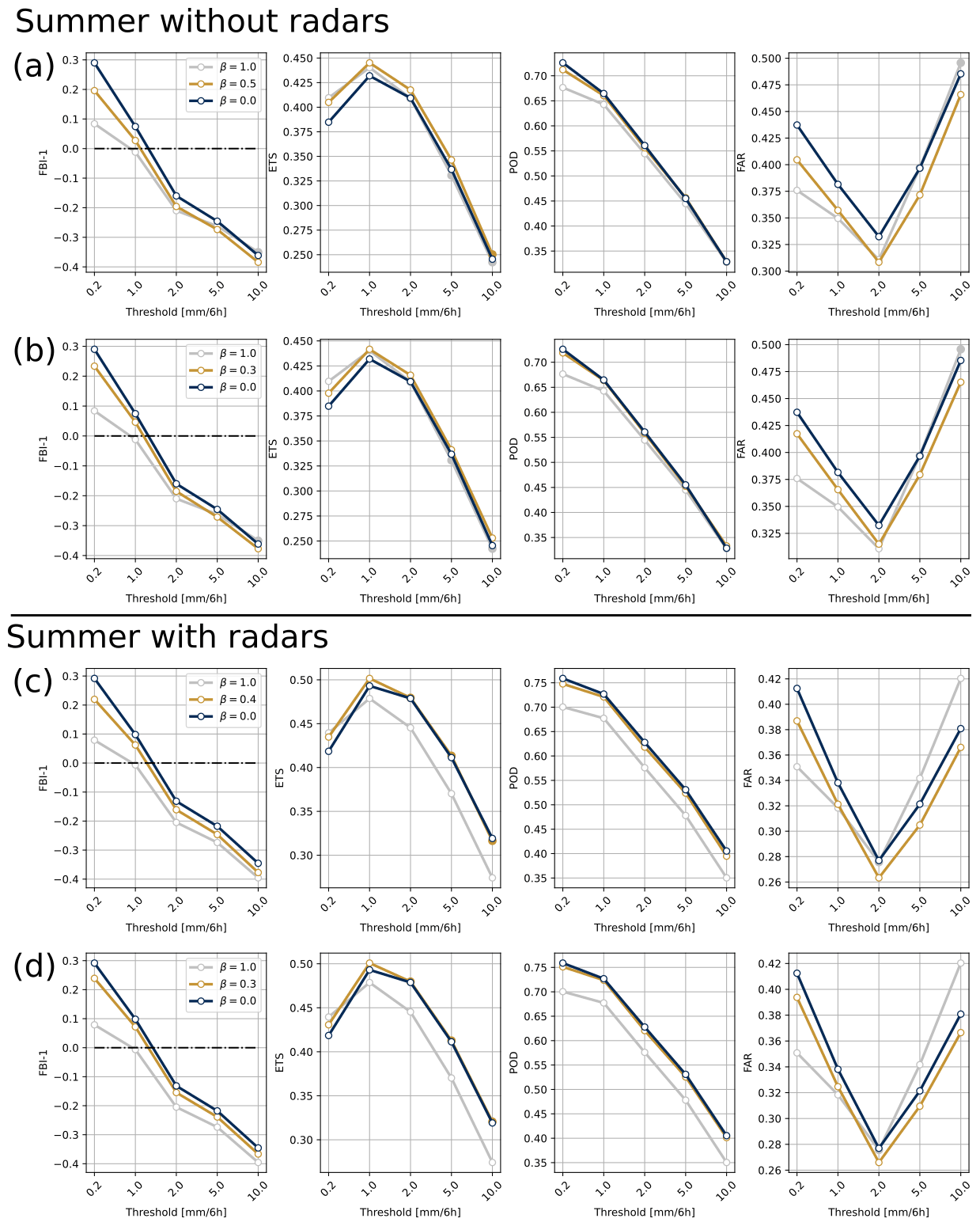
Figure 3Panels (a) and (b) show the FBI-1, ETS, POD, and FAR across the whole domain for the summer experiment without radar QPEs for precipitation analysis with β=0.0 (dark blue line), β=1.0 (gray line), β=0.5 (yellow lines in a), and β=0.3 (yellow lines in b). Panels (c) and (d) are the same figures but for the summer experiment with the assimilation of radar QPEs with β=1.0 (gray lines), β=0.4 (yellow lines in c), and β=0.3 (yellow lines in d), with all three compared to the reference experiment when β=0.0 (blue lines). Filled markers indicate no significant differences (at the 95 % confidence level) between the reference experiment β=0.0 and the β=1.0, β=0.5, β=0.4, or β=0.3 experiments.
The results for the analysis during the same season but with the assimilation of the radar QPEs are showed in Fig. 3c and d. Similarly to what was observed for the NRMSE values, all metrics were generally improved when assimilating the radar QPEs, but the differences between the reference and the optimal β=0.4 were less pronounced. The analysis with β=0.4 showed significantly reduced FARs for all thresholds. However, the improvement in the ETS when compared to the β=0.0 was significant only for small thresholds (0.2 and 1.0 mm). For higher thresholds, the skill was slightly improved, but this improvement was not significant at the 95 % confidence level. Similarly to the experiment without radar QPEs (Fig. 3a, b), the POD slightly deteriorated, and the FBI-1 decreased for small precipitation events but increased for events of medium to high intensity. The dynamic approach, β=1.0, showed a different pattern when assimilating radar datasets. Almost all scores and thresholds were significantly degraded compared with β=0.0 and β=0.4. The only improvement was seen for precipitation events above 0.2 mm, but the degradation for other thresholds was too substantial. The use of β=0.3 seemed again to be a good compromise regarding the bias, as it reduced the analysis smoothness when compared with β=0.4 while also preventing POD deterioration.
Finally, Fig. 4a illustrates the same metrics during the winter and compares β=0.7 and β=1.0 to the reference experiment. With β=0.7, the ETS was significantly improved, and the false alarms at the 95 % confidence level were reduced. Fewer precipitation events were generated for all selected thresholds with the analysis using β=0.7 compared with β=0.0. Again, this improves the performance for 6 h precipitation greater than 0.2 and 1.0 mm but not for accumulations greater than 2.0 mm. However, the degradation of the FBI-1 for high-intensity precipitation was much less pronounced than in summer, especially for such a high β value. The probability of detecting events (POD score) greater than 0.2 mm was significantly reduced, but it was increased for heavy precipitation events (>10 mm). Moderate performance was obtained for the experiment with β=1.0; this experiment did no better than when using β=0.7, but the two experiments were not that different for several thresholds and scores (e.g., FBI-1 for precipitation above 0.2 mm in Fig. 3a).
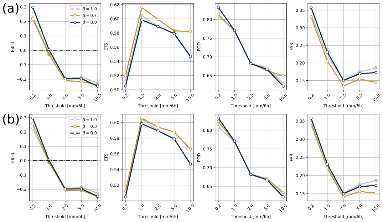
Figure 4Same as Fig. 3 but for the winter experiment with β=0.7 (a), β=0.3 (b), and β=1.0 (a, b), with all three compared to the reference experiment (β=0.0).
For the sake of comparison with the summer season, contingency table metrics using β=0.3 are also displayed in Fig. 4b. It appeared that this value also provides improved metrics even though it was not identified as optimal. Indeed, the FBI-1 was still, although to a lesser extent, reduced for precipitation above 0.2 mm compared with the reference experiment. It is interesting to note that the degradation of the FBI-1 was less pronounced for other thresholds and was not significant in most cases. Similarly, the POD degradation for the 0.2 mm threshold was less pronounced. The ETS and FAR were still significantly improved for all thresholds relative to the reference experiment, although to a lesser extent than with β=0.7.
In light of these results, the optimal β value identified through the use of the NRMSE showed improved performance compared with the static (β=0.0) and dynamic (β=1.0) configurations. Improved skill and reduced FARs were indeed obtained when using the optimal β for both the summer and winter experiments. However, the frequency of moderate- to high-intensity 6 h precipitation was reduced, especially in summer. The latter can be detrimental to very localized high-intensity precipitation events. The examination of the same scores for other values of β highlighted that β=0.3 offered a good compromise between skill gain and not overly damaging the frequency bias for high-intensity precipitation events for both seasons. For these reasons, β=0.3 was maintained as optimal in the sense of the abovementioned compromise and is used for the additional checks presented below.
7.3 Verification against ST4
The impact of radar QPE assimilation in the hybrid approach has been demonstrated in the previous sections. Therefore, to simplify the discussion, the comparison of CaPA analyses with ST4 is only performed for the experiments that assimilated the ground-based radars (i.e., excluding the summer experiment without radar QPE). This point is also justified by the fact that the operational CaPA is integrated with the radar QPEs and that the final objective is a comparison with this system. Thus, in the following, the summer experiments refer to the one that assimilates the radar QPEs.
Figure 5 shows the accumulated precipitation for ST4 and CaPA using β=0.3 and the differences between these two datasets. More spatial patterns and higher summer precipitation amounts were observed in ST4 than in the CaPA using β=0.3 (Fig. 5a). The higher native resolution of ST4 and the limited ability of the CaPA background model to predict convective precipitation, especially at the 10 km grid spacing, may explain such results.
Figure 5Panel (a) displays the 6 h precipitation accumulated over the summer for ST4 (left), for CaPA with β=0.3 (middle), and the difference between the two (right). Panel (b) is the same as panel (a) but for the winter experiment.
The winter (Fig. 5b), generally characterized by spatially larger precipitation events, showed a better agreement between CaPA and ST4. Indeed, ST4 and CaPA with β=0.3 had similar spatial patterns with both over- and underestimated accumulations depending on the location, although to a lesser extent than in summer. These results can be interpreted both by the greater forecasting capacity of the background model in winter and by the expected lower impact of the horizontal resolution during this season. Accumulated precipitation, using either β=0.0 or β=0.3, was compared to ST4 at the grid-point scale to identify the best parameter (not shown for conciseness). It was found that, without spatial consistency, some locations (grid cells) were better represented with β=0.3, while β=0.0 was more suitable for other locations. Therefore, moving from β=0.0 to β=0.3 has a minimal impact on seasonal precipitation accumulations.
Figures 6a and b depict the fraction of grid cells above selected 6 h thresholds averaged for the summer and winter, respectively. During summer, the differences between the configurations with β=0.0 and β=0.3 were very small (<2 %), as shown by the very close yellow and blue curves. Consistent with results on the FBI-1 (Fig. 3), the fraction of precipitation events above 0.2 mm generated in the analysis using β=0.0 or β=0.3 were slightly higher than in ST4 for both season. During summer, the fraction of grid points greater than 1, 2, and 5 mm per 6 h period were systematically underestimated by 2 % to 3 % in CaPA compared with ST4, and these fractions appear to contribute importantly to the underestimation of the ST4 precipitation totals (Fig. 6). Winter was similar (Fig. 6b), as fractions of grid cells for the 6 h precipitation analysis were generally overestimated in the analysis. However, this overestimation was relatively smaller (<1 %) than summer and became almost negligible for the 5 and 10 mm per 6 h thresholds.
Figure 6The fractional areal coverage (%) of the 6 h accumulated precipitation meeting or exceeding selected thresholds (x axis) during the summer (a) and the winter (b) for ST4 (dashed black line) and CaPA using the configuration with β=0.0 (blue line) and β=0.3 (yellow line) over their common domain (Fig. 5).
The FSSs for the 11 analyses differing by β values and using ST4 as a reference were calculated for the 0.2 and 1.0 mm per 6 h thresholds with neighborhood length scales of 20, 30, and 50 km (Fig. 7). For a given neighborhood length scale and for the 0.2 mm threshold during the summer (Fig. 7a), the FSS increased when β went from 0.0 to 0.5 and then decreased for higher β values, consistent with the results obtained for the NRMSE values. Similarly, during the winter and for the same threshold, FSS values increased when β went from 0.0 to 0.7 and decreased thereafter (Fig. 7c). The gain associated with the use of β>0.0 was less marked for the 1.0 mm threshold, especially for the summer (Fig. 7b). These results are consistent with those obtained with scores based on the contingency tables for the summer experiment. For both seasons (Fig. 7b, d), the use of β=0.3 did not, however, deteriorate the FSS values compared to those of the reference experiment, and they even showed a slight improvement during the winter.

Figure 7The fraction skill score (FSS) as a function of the different β values for the 6 h precipitation meeting or exceeding the 0.2 mm (a, c) and 1.0 mm (b, d) thresholds for summer (a, b) and winter (c, d), using ST4 precipitation as reference. Each curve represents a different neighboring length scale (20, 30, or 40 km).
Figure 8The precipitation field (a, d) from CaPA and the associated CFIA values (b, e) for 5 and 18 January 2020, both valid at 12:00 UTC. Panels (c) and (f) show the CFIA for the same date but using the hybrid approach with a high contribution of the REPS – here with β=0.7.
7.4 Confidence index
In the OI-based CaPA, CFIA fields are characterized by circular structures, as shown for two winter cases in Fig. 8b. Small dots of high values are centered around the surface stations, and large disks represent radar footprints. These particular structures are a direct consequence of the assumptions on the error isotropy.
Using the hybrid approach in CaPA enables one to account for flow-dependent errors, allowing CFIA spatial distributions to be linked to meteorological situations and, thus, lessening the influence of the aforementioned assumptions. However, in this configuration, the variances of the background field errors are also spatially variable, in contrast to the spatially constant value used for operational CaPA (Eqs. 4, 9). Therefore, this makes the interpretability of CFIA, in its current definition (Eq. 11), less straightforward. To illustrate this point, two different meteorological situations were selected and are illustrated in Fig. 8a and d. The 6 h precipitation fields for 5 January 2020 (Fig. 8a) and 18 January 2020 (Fig. 8d) valid at 12:00 UTC were both characterized by large synoptic events but at different locations. Increasing the contribution of the REPS in the analysis computation, β=0.7 in Fig. 8c and f, leads to CFIA values following meteorological spatial distributions. Generally, CFIA values tended to be higher at places with precipitation than when using β=0.0, as shown in the eastern part of the domain for the 18 January case (Fig. 8f). Inversely, locations with no precipitation in the background field tended to show small CFIA values. This last result is consistent with the calculation of Pbd (Eq. 5), which, when the ensemble members have no or very little precipitation, will tend to a zero matrix. Nonetheless, CFIA remained close to zero above the Atlantic Ocean for the case of 5 January (Fig. 8c) despite the synoptic event that occurred in that location. This is explained by the current CaPA computation framework. No matter the value of β, analysis precipitation at a given grid cell is equal to the background when no observations are available to be assimilated in the vicinity. This leads to error variances of the analysis () being close to those of the background (); thus, by construction, CFIA will tend towards small values (Eq. 11). As a result, the current CFIA (Eq. 11) revealed two limitations for the hybrid assimilation approach: (i) users interested in grid cells with high CFIA values may indirectly favor locations with precipitation, which, in turn, can lead to biased interpretation, and (ii) low CFIA values may have two different interpretations. To overcome the first limitation, a field representing the density of assimilated observations for each grid cell will come along with the CaPA precipitation fields. In addition, to ease CFIA interpretation, the reference, which is currently in Eq. (11), will be exchanged with a temporal climatology of the background field errors. To do this, the denominator in Eq. (11) will be replaced by the time average of , calculated for each grid cell using an exponential filter that gives more weight to the most recent cases. Different tests made on CFIA estimates are beyond the scope of this paper and will be discussed in a different study.
Based on optimal interpolation, the Canadian Precipitation Analysis (CaPA), currently operational at CCMEP, is used for different applications (see Fortin et al., 2018, for further details). The recently available operational 20-member REPS with a ∼10 km grid spacing naturally led to an examination of whether it was possible to improve the estimation of background error covariances used by the current CaPA OI. From this perspective, the selected approach is a so-called hybrid approach (Hamill and Snyder, 2000; Counillon et al., 2009), and it consists of a weighting of two covariance matrices: one obtained by OI and the other by an ensemble Kalman filter based on the REPS. The primary motivation is to overcome some simplifying assumptions about the structure of background errors when using OI. Indeed, the operational CaPA uses a spatial covariance structure of background errors assumed to be isotropic and is modeled as an exponential function. The second motivation is the documented positive impact of this approach for domains with low observation density, which is the case for some regions of the CaPA domain (e.g., northern Canada) and during the winter season when few stations are assimilated.
In practice, this consists of choosing an optimal weighting between two covariance matrices of background field errors, one from OI and the other from REPS, through a parameter – β – which varies between zero and one. The experiments were conducted for 6 h precipitation accumulations and over two seasons, summer 2019 and winter 2020. To verify the impact of the amount of assimilated observations, an additional experiment without radar QPE assimilation was conducted for summer 2019. This additional experiment was not performed for winter, as the assimilated radar QPEs during the solid precipitation season are anyway negligible in CaPA (Fortin et al., 2015).
First, results have shown that the analysis with the assimilation of the radar QPEs limits the positive impacts of the increase of the weighting towards the REPS (i.e., high β values). Indeed, with and without radar QPE assimilation and according to NRMSE estimates, summer had optimal β values of 0.4 and 0.5, respectively. Winter precipitation showed higher optimal values of β, around 0.7, meaning that a higher weighting in favor of the REPS is preferable during that season. This result confirmed the known positive impact of the hybrid method in a low-station-density configuration. The second reason is the higher forecasting skill of the background model (RDPS) and the REPS during the winter season, leading to a better error specification. Interestingly, these optimal values obtained when comparing precipitation from surface stations to the analysis (in a leave-one-out framework) were consistent with those obtained with the FSSs, using a relatively independent observation dataset and on a smaller domain – the Stage IV analysis (Lin and Mitchell, 2005).
The use of the hybrid approach with optimal β values for each experiment increased the analysis skill of both the operational CaPA (β=0.0) and a purely dynamic approach (β=1.0). This result is especially true for low-intensity precipitation events, for which the FAR has been significantly reduced. In summer, the frequency bias score was improved for small precipitation events (up to 1 mm) but degraded for higher thresholds. High-intensity precipitation events were indeed smoothed when using the optimal β value. This result was also observed for the winter, although to a lesser extent. Using a trade-off value of β=0.3 for the summer experiments reduced the impact of smoothing high-intensity events while allowing for significant skill improvement. According to the winter 2020 experiment results, a higher β would have been more suitable. However, in practice, this means choosing a date in the CaPA configuration for which β must be modified. A more extended test period and further experiments would be needed to distinguish whether the parameter changes should be made during the regular North American domain seasons or during precipitation phase changes (approximately in May and October). In the meantime, other tests, using β=0.3 during the winter, have provided acceptable skill and bias results while being conservative.
Different flavors of the hybrid approach have also been tested but have not been developed in this article as they did not contribute positively or significantly to the selected metrics. As suggested in Counillon et al. (2009), an inflation factor ranging from 1.0 to 2.0 was applied to alleviate the possible lack of spread in the REPS, but the experiments showed no or negative impacts on the verification metrics. Another hybrid configuration was also conducted to mitigate the impact of the smoothing of high-intensity events during summer precipitation. For that test, the hybrid approach was activated only if at least half of the REPS members had strictly positive precipitation; otherwise, β was set to zero. The resulting scores showed higher biases for low-intensity precipitation events than the current approach and no bias reduction for high-intensity events.
In addition to the work planned for a better specification of the CFIA (Sect. 7.4), future developments should focus on improving the current hybrid approach by accounting for the observation density when selecting the optimal β values (i.e., allow for spatial variability of β). Therefore, the hybrid system could benefit places without observations while not degrading the analysis at locations with a high density of observations. This task will be facilitated by the availability of a new field providing information on the amount of data assimilated (Sect. 7.4). Other works should explore the possibility of extending the current approach to create an ensemble version of the precipitation analysis. The REPS members, with prior bias corrections, could be used to create the analysis background field members. The hybrid approach could also help create a global version of CaPA using the Global Deterministic Prediction System (GDPS) and the GEPS (Houtekamer et al., 2014) as a background model and an ensemble system, respectively. A global version of CaPA has already been identified as useful for land surface data assimilation at CCMEP. In that context, the hybrid approach would be especially relevant for the many regions of the world that do not benefit from high-density precipitation observations.
REPS and CaPA (regional configuration) are both available as ECCC operational systems from the following respective locations: https://dd.meteo.gc.ca/ensemble/reps/10km/grib2 (ECCC, 2022a) and https://dd.meteo.gc.ca/analysis/precip/rdpa/grib2/polar_stereographic (ECCC, 2022b). The output data from this study (CaPA using hybrid methodology for the assimilation) have been archived and are available upon request from the corresponding author.
The main contributions from each co-author are as follows: under the supervision of SB and VF, DK proposed the methodology, the experimental design, and the preparation of the paper; GR contributed to the adaptation of the CaPA data assimilation code to integrate the hybrid modeling; and VF, SB, and FL contributed to interpreting results and paper preparation.
The contact author has declared that none of the authors has any competing interests.
Publisher’s note: Copernicus Publications remains neutral with regard to jurisdictional claims in published maps and institutional affiliations.
This paper was edited by Pierre Tandeo and reviewed by two anonymous referees.
Bachmann, K., Keil, C., and Weissmann, M.: Impact of radar data assimilation and orography on predictability of deep convection, Q. J. Roy. Meteor. Soc., 145, 117–130, https://doi.org/10.1002/qj.3412, 2019. a
Bonavita, M., Hamrud, M., and Isaksen, L.: EnKF and Hybrid Gain Ensemble Data Assimilation. Part II: EnKF and Hybrid Gain Results, Mon. Weather Rev., 143, 4865–4882, https://doi.org/10.1175/MWR-D-15-0071.1, 2015. a
Brown, J. D., Seo, D.-J., and Du, J.: Verification of Precipitation Forecasts from NCEP's Short-Range Ensemble Forecast (SREF) System with Reference to Ensemble Streamflow Prediction Using Lumped Hydrologic Models, J. Hydrometeorol., 13, 808–836, https://doi.org/10.1175/JHM-D-11-036.1, 2012. a
Buizza, R.: Ensemble forecasting and the need for calibration, in: Statistical Postprocessing of Ensemble Forecasts, edited by: Vannitsem, S., Messner, J. W., and Wilks, D. S., Elsevier, 15–48, ISBN: 978-0-12-812372-0, 2019. a, b
Caron, J.-F., Milewski, T., Buehner, M., Fillion, L., Reszka, M., Macpherson, S., and St-James, J.: Implementation of Deterministic Weather Forecasting Systems Based on Ensemble–Variational Data Assimilation at Environment Canada. Part II: The Regional System, Mon. Weather Rev., 143, 2560–2580, 2015. a, b
Charron, M., Pellerin, G., Spacek, L., Houtekamer, P., Gagnon, N., Mitchell, H. L., and Michelin, L.: Toward random sampling of model error in the Canadian ensemble prediction system, Mon. Weather Rev., 138, 1877–1901, 2010. a, b
Counillon, F., Sakov, P., and Bertino, L.: Application of a hybrid EnKF-OI to ocean forecasting, Ocean Sci., 5, 389–401, https://doi.org/10.5194/os-5-389-2009, 2009. a, b, c, d
Cressie, N.: Statistics for Spatial Data, Revised Edition, Wiley Classics Library, John Wiley & Sons, ISBN: 978-1-119-11461-1, 2015. a
Ebert, E.: Ability of a poor man's ensemble to predict the probability and distribution of precipitation, Mon. Weather Rev., 129, 2461–2480, 2001. a
ECCC: Regional Ensemble Prediction System (REPS) Version 3.0.0 Summary of changes with respect to version 2.4.0 and validation, Dorval, Qc, Canada, Tech. rep., https://collaboration.cmc.ec.gc.ca/cmc/cmoi/product_guide/docs/lib/technote_reps-300_20190703_e.pdf (last access: 28 September 2022), 2019. a
ECCC: Index of /ensemble/reps/10km/grib2, Government of Canada [data set], https://dd.meteo.gc.ca/ensemble/reps/10km/grib2, last access: 28 September 2022a. a
ECCC: Index of /analysis/precip/rdpa/grib2/polar_stereographic, Government of Canada [data set], https://dd.meteo.gc.ca/analysis/precip/rdpa/grib2/polar_stereographic, last access: 28 September 2022b. a
Evans, A. M.: Investigation of enhancements to two fundamental components of the statistical interpolation method used by the Canadian Precipitation Analysis (CaPA), MS thesis, University of Manitoba,Winnipeg, Manitoba, https://mspace.lib.umanitoba.ca/xmlui/handle/1993/22276 (last access: 28 September 2022), 2013. a
Evensen, G.: The ensemble Kalman filter: Theoretical formulation and practical implementation, Ocean Dynam., 53, 343–367, https://doi.org/10.1007/s10236-003-0036-9, 2003. a
Fortin, V., Roy, G., Donaldson, N., and Mahidjiba, A.: Assimilation of radar quantitative precipitation estimations in the Canadian Precipitation Analysis (CaPA), J. Hydrol., 531, 296–307, https://doi.org/10.1016/j.jhydrol.2015.08.003, 2015. a, b, c, d, e, f, g, h, i, j, k, l
Fortin, V., Roy, G., Stadnyk, T., Koenig, K., Gasset, N., and Mahidjiba, A.: Ten Years of Science Based on the Canadian Precipitation Analysis: A CaPA System Overview and Literature Review, Atmos. Ocean, 56, 178–196, https://doi.org/10.1080/07055900.2018.1474728, 2018. a, b
Hamill, T. M. and Snyder, C.: A hybrid ensemble Kalman filter–3D variational analysis scheme, Mon. Weather Rev., 128, 2905–2919, https://doi.org/10.1175/1520-0493(2000)128<2905:AHEKFV>2.0.CO;2, 2000. a, b, c, d, e, f, g
Houtekamer, P. and Zhang, F.: Review of the Ensemble Kalman Filter for atmospheric data assimilation, Mon. Weather Rev., 144, 4489–4532, https://doi.org/10.1175/MWR-D-15-0440.1, 2016. a, b
Houtekamer, P. L. and Mitchell, H. L.: Data assimilation using an Ensemble Kalman Filter technique, Mon. Weather Rev., 126, 796–811, https://doi.org/10.1175/1520-0493(1998)126<0796:DAUAEK>2.0.CO;2, 1998. a, b
Houtekamer, P. L., Deng, X., Mitchell, H. L., Baek, S.-J., and Gagnon, N.: Higher Resolution in an Operational Ensemble Kalman Filter, Mon. Weather Rev., 142, 1143–1162, https://doi.org/10.1175/MWR-D-13-00138.1, 2014. a, b
Houtekamer, P. L., Buehner, M., and De La Chevrotière, M.: Using the hybrid gain algorithm to sample data assimilation uncertainty, Q. J. Roy. Meteorol. Soc., 145, 35–56, https://doi.org/10.1002/qj.3426, 2019. a, b
Jacques, D., Michelson, D., Caron, J. F., , and Fillion, L.: Latent heat nudging in the Canadian Regional Deterministic Prediction System, Mon. Weather Rev., 146, 3995–4014, https://doi.org/10.1175/MWR-D-18-0118.1, 2018. a
Kalnay, E., Li, H., Miyoshi, T., Yang, S.-C., and Ballabrera-Poy, J.: 4D-Var or ensemble Kalman filter?, Tellus A, 59, 758–773, https://doi.org/10.1111/j.1600-0870.2007.00261.x, 2007. a
Kleist, D. T. and Ide, K.: An OSSE-Based Evaluation of Hybrid Variational–Ensemble Data Assimilation for the NCEP GFS. Part I: System Description and 3D-Hybrid Results, Mon. Weather Rev., 143, 433–451, https://doi.org/10.1175/MWR-D-13-00351.1, 2015. a
Kollias, P., Bharadwaj, N., Clothiaux, E. E., Lamer, K., Oue, M., Hardin, J., Isom, B., Lindenmaier, I., Matthews, A., Luke, E. P., Giangrande, S. E., Johnson, K., Collis, S., Comstock, J., and Mather, J. H.: The ARM Radar Network: At the Leading-edge of Cloud and Precipitation Observations, B. Am. Meteorol. Soc., 101, E588–E607, https://doi.org/10.1175/BAMS-D-18-0288.1, 2020. a
Lespinas, F., Fortin, V., Roy, G., Rasmussen, P., and Stadnyk, T.: Performance Evaluation of the Canadian Precipitation Analysis (CaPA), J. Hydrometeorol., 16, 2045–2064, https://doi.org/10.1175/JHM-D-14-0191.1, 2015. a, b, c, d, e, f, g, h, i
Lin, Y. and Mitchell, K.: The NCEP Stage II/IV hourly precipitation analyses: development and applications, in: Preprints of the 19th Conference on Hydrology, American Meteorological Society, San Diego, CA, 9–13 January 2005, 1–3, https://www.google.com/url2ahUKEwjXvYQ (last access: 28 September 2022), 2005. a, b
Lorenz, E. N.: Deterministic nonperiodic flow, J. Atmos. Sci., 20, 130–141, 1963. a
Mahfouf, J., Brasnett, B., and Gagnon, S.: A Canadian Precipitation Analysis (CaPA) project: Description and preliminary results, Atmos. Ocean, 45, 1–17, https://doi.org/10.3137/ao.v450101, 2007. a
Nelson, B. R., Prat, O. P., Seo, D. J., and Habib, E.: Assessment and implications of NCEP stage IV quantitative precipitation estimates for product intercomparisons, Weather Forecast., 31, 371–394, https://doi.org/10.1175/WAF-D-14-00112.1, 2016. a
Penny, S. G., Behringer, D. W., Carton, J. A., and Kalnay, E.: A Hybrid Global Ocean Data Assimilation System at NCEP, Mon. Weather Rev., 143, 4660–4677, https://doi.org/10.1175/MWR-D-14-00376.1, 2015. a
Rasmussen, R., Baker, B., Kochendorfer, J., Meyers, T., Landolt, S., Fischer, A. P., Black, J., Thériault, J. M., Kucera, P., Gochis, D., Smith, C., Nitu, R., Hall, M., Ikeda, K., and Gutmann, E.: How well are we measuring snow: The NOAA/FAA/NCAR winter precipitation test bed, B. Am. Meteorol. Soc., 93, 811–829, 2012. a
Roberts, N. M. and Lean, H. W.: Scale-Selective Verification of Rainfall Accumulations from High-Resolution Forecasts of Convective Events, Mon. Weather Rev., 136, 78–97, https://doi.org/10.1175/2007MWR2123.1, 2008. a
Schwartz, C. S., Kain, J. S., Weiss, S. J., Xue, M., Bright, D. R., Kong, F., Thomas, K. W., Levit, J. J., and Coniglio, M. C.: Next-Day Convection-Allowing WRF Model Guidance: A Second Look at 2-km versus 4-km Grid Spacing, Mon. Weather Rev., 137, 3351–3372, https://doi.org/10.1175/2009MWR2924.1, 2009. a
Wang, X., Hamill, T. M., Whitaker, J. S., and Bishop, C. H.: A Comparison of Hybrid Ensemble Transform Kalman Filter – Optimum Interpolation and Ensemble Square Root Filter Analysis Schemes, Mon. Weather Rev., 135, 1055–1076, https://doi.org/10.1175/MWR3307.1, 2007. a, b
Wang, X., Barker, D. M., Snyder, C., and Hamill, T. M.: A hybrid ETKF–3DVAR data assimilation scheme for the WRF model. Part I: Observing system simulation experiment, Mon. Weather Rev., 136, 5116–5131, https://doi.org/10.1175/2008MWR2444.1, 2008a. a, b, c, d, e, f
Wang, X., Barker, D. M., Snyder, C., and Hamill, T. M.: A Hybrid ETKF–3DVAR Data Assimilation Scheme for the WRF Model. Part II: Real Observation Experiments, Mon. Weather Rev., 136, 5132–5147, https://doi.org/10.1175/2008MWR2445.1, 2008b. a, b