the Creative Commons Attribution 4.0 License.
the Creative Commons Attribution 4.0 License.
 | 07 Apr 2022
Estimate of energy loss from internal solitary waves breaking on slopes
Kateryna Terletska
Vladimir Maderich
Internal solitary waves (ISWs) emerge in the ocean and seas in various forms and break on the shelf zones in a variety of ways. This results in intensive mixing that affects processes such as biological productivity and sediment transport. As ISWs of depression propagate in a two-layer ocean, from the deep part onto a shelf, two mechanisms are significant: (1) the breaking of internal waves over bottom topography when fluid velocities exceed the wave phase speed that causes overturning of the rear face of the wave, and (2) the changing of polarity at the turning point where the depths of the upper and lower layers are equal. We assume that the parameters that describe the process of the interaction of ISWs in a two-layer fluid with an idealized shelf-slope topography are (1) the nondimensional wave amplitude, normalized on the upper-layer thickness; (2) the ratio of the height of the bottom layer on the shelf to the incident wave amplitude; and (3) the angle of the bottom inclination. Based on a proposed three-dimensional classification diagram, four types of wave propagation over the slopes are distinguished: the ISW propagates over the slope without changing polarity and wave breaking, the ISW changes polarity over the slope without wave breaking, the ISW breaks over the slope without changing polarity, and the ISW both breaks and changes polarity over the slope. The energy loss during ISW transformation over slopes with various angles was estimated using the results of 85 numerical experiments. “Hot spots” of high levels of energy loss were highlighted for an idealized bottom configuration that mimics the continental shelf in the Lufeng region in the South China Sea.
- Article
(3433 KB) - Full-text XML
- BibTeX
- EndNote


Observations demonstrate evidence of internal solitary waves (ISWs) in coastal oceans and seas (Apel et al., 1995). It is generally accepted that one of the main causes of ISWs is the barotropic tide interacting with the bottom topography (Maxworthy, 1979; Gerkema and Zimmerman, 1995).
Generated by tides, ISWs of depression (where the upper-layer thickness is usually much less than the depth of the ocean) are the most energetic and can propagate thousands of kilometers from their origin (Kunze et al., 2012). As a result, ISWs transport energy far from the location of their generation. Like surface waves, internal waves break at the coastal zone of the ocean. Such waves are an important component of mixing and energy dissipation in the ocean (Liu et al., 1998; Davis et al., 2020). The breaking of ISWs upon sloping boundaries in the coastal region also plays an important role in diapycnal mixing (St. Laurent et al., 2012), biological enhancement (Sangrà et al., 2001; Wang et al., 2007), and resuspension of bottom deposits (Pomar et al., 2012; Boegman and Stastna, 2019).
The interaction behavior of ISWs depends on the steepness of the topography and the characteristics of the solitary waves (Garrett and Kunze, 2007). If the slopes are smooth, much of the energy scatters upslope onto the continental shelf where it will dissipate; however, if the slopes are steeper, energy will reflect and return to the deep ocean (Klymak et al., 2010). It is important to understand the mechanisms of the transformation of ISWs at continental slopes and identify “hot spots” of wave energy dissipation. Two shoaling mechanisms can be important: (1) the conversion of ISWs of depression into elevation waves in a two-layer stratification when the thickness of the upper mixed layer is greater than one-half of the total water depth (Helfrich and Melville, 1986; Cheng et al., 2011; Bai et al., 2021); and (ii) ISW breaking on the slope that occurs when fluid velocities in the wave exceed the wave phase speed, which leads to the overturning of the rear face of the wave, shear instability, and intensive mixing. Different types of breaking are commonly distinguished by slope inclination, water column stratification, and wave characteristics. Assuming analogy with surface waves, the breaking regimes of ISWs in a two-layer fluid over a slope have been classified (Aghsaee et al., 2010; Boegman et al., 2005) into surging, plunging, collapsing, and fission. In these studies, the classification of breaking is based on the Iribarren number, which is a ratio of the slope to the square root of the wave steepness (amplitude divided by the wavelength). This criterion was modified by Nakayama et al. (2019) for collapsing and plunging breakers using a new wave Reynolds number that takes nonlinear wave steepening into account. A simple three-dimensional α β γ classification diagram was proposed by Terletska et al. (2020) to distinguish different regimes of ISW interactions with the shelf-slope topography. The classification is based on three parameters: the slope angle γ; the nondimensional wave amplitude α (wave amplitude normalized on the upper-layer thickness); and the blocking parameter β, which is the ratio of the height of the bottom layer of the shelf to the incident wave amplitude.
ISWs breaking over slopes have been observed in many coastal locations worldwide (New and Pingree, 1990; Alford et al., 2015; Vlasenko et al., 2014; Osborn et al., 1980; Nam and Send, 2011; Fu et al., 2016; Orr and Mignerey, 2003; Klymak et al., 2006). Observational studies have also shown that the amplitudes of depression ISWs in the South China Sea (SCS) could reach extreme values of over 200 m (Huang et al., 2016; Ramp et al., 2010; Klymak et al., 2010). Based on the analysis of satellite images (Wang et al., 2013; Jackson, 2004), it has been found that most internal waves in the northeastern South China Sea are generated in the Luzon Strait. Further, solitary waves propagate westward and then diffract around the Dongsha Atoll. In the shallow-water regions of the northern SCS, changes in water depth may cause polarity conversion, leading to the transformation of depression ISWs into elevation ISWs (Liu et al., 1998). Orr and Mignerey (2003) showed that the kinetic energy of ISWs decreased three times after changing polarity, while Zhang et al. (2018) showed that the seasonal variations in stratification caused these seasonal variations in polarity. The present study is focused on ISW transformation over an idealized shelf-slope topography with a two-layer stratification. The objectives of this work are (1) to compare α β γ classification with the results of numerical modeling, laboratory studies, and field observations; (2) to identify high-energy-dissipation zones of ISWs that pass over the shelf-slope topography using the α, β, γ classification; (3) to apply the α, β, γ classification to numerical modeling data that mimic ISW transformation over a continental shelf in the Lufeng region (SCS); and (4) to determine energy loss as a result of the transformation of ISWs over the shelf-slope topography. Information about polarity change criteria and breaking criteria in the α β γ classification of ISW transformation regimes over shelf topography is presented in Sect. 2. An overview of field and laboratory measurement data and their comparison with the numerical modeling data are given in Sect. 3. The energy dissipation of ISWs breaking over shelf topography is considered in Sect. 4. Finally, the results are summarized in the Sect. 5.
A two-layer approximation is a simple model of stably stratified oceans and lakes. In this model, we approximated stratification using two continuous layers of depths h1 (upper layer) and h2 (lower layer) with a relatively thin pycnocline. When h1>h2, ISWs propagate in the form of elevation ISWs, whereas if h1<h2, they propagate in the form of waves of depression. In this study, we consider ISWs of depression (with amplitude ain) propagating over an idealized shelf slope with a slope γ and a minimum depth of the lower layer over the shelf of h2+. The idealized shelf-slope topography is shown in Fig. 1b, and the idealized configuration that mimics the continental shelf in the Lufeng region (Fig. 1a) in the SCS is shown in Fig. 1c.
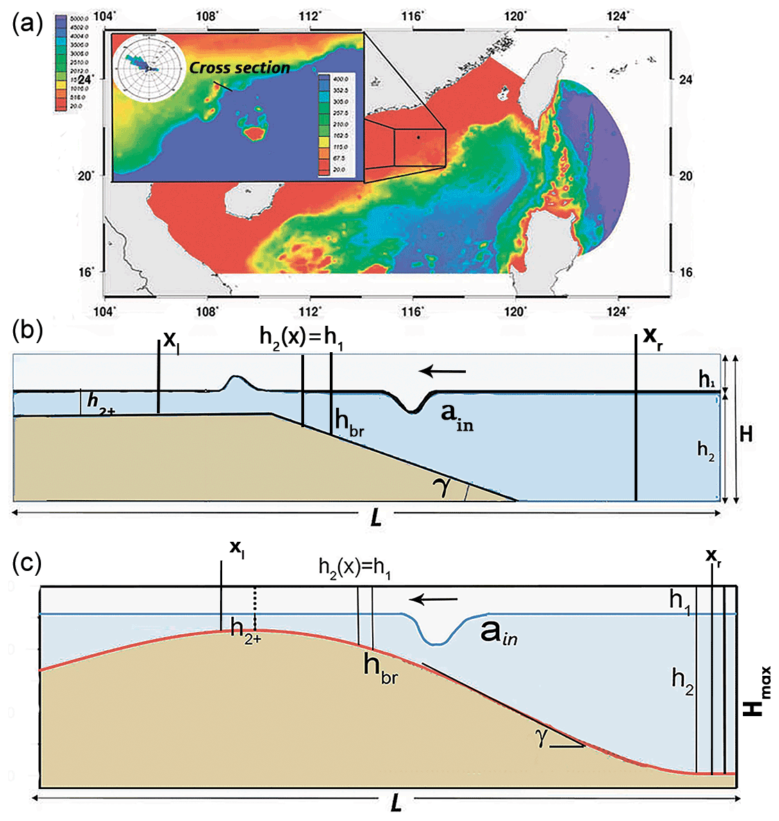
Figure 1Sketch of the transformation of a depression ISW over a shelf slope. Panel (a) shows the Lufeng region in the South China Sea, panel (b) is a sketch of wave breaking and the changing of the polarity of an ISW of depression after passing through a turning point, and panel (c) displays the idealized topography in the Lufeng region.
It was assumed that ISW transformation over a slope is controlled by stratification, slope inclination, and amplitudes (wavelength) of the incident wave (Terletska et al., 2020). Two possibilities that could occur with the wave during shoaling were determined: (i) ISW breaking, which was associated with gravitational instability due to the wave overturning and shear instability, and (ii) changing ISW polarity on the slope.
Three parameters, α, β, and γ, can be important for the behavior of the incident wave on a shelf slope (Fig. 1b, c):
-
the slope inclination γ, which is measured as an angle;
-
the blocking parameter β, which is the ratio of the height of the minimum depth of the lower layer over the shelf h2+ (Fig. 1b, c) to the incident wave amplitude ain, calculated as
-
the nonlinearity parameter, which is the ratio of the incident wave amplitude to the depth of upper layer, calculated as
The idea for the blocking parameter β comes from numerical and laboratory experiments as the “degree of blocking”, which is an important parameter that controls the loss of energy into transmitted and reflected waves passing an obstacle (Vlasenko and Hutter, 2002; Wessels and Hutter, 1996). Parameter β was modified by Talipova et al. (2013), who considered ISWs (as depression and elevation types) passing over a step (γ=90∘). It was shown that the transformation of an ISW of depression over an underwater step is weak for β>3 (when the dynamics of the ISW could be described by weakly nonlinear theory); for , the interaction is moderate (when the main mechanism for ISW breaking over a bottom step produces shear instability); for , the interaction is strong, with maximal energy loss, and the ISW produces a flow that results in jets and vortices. Interaction in the range is called the “transitional regime”, as it represents the step height between strong interaction and full reflection from the step, whereas full reflection from the underwater step takes place for .
Internal waves in the framework of weakly nonlinear theory change their polarity at the point where the upper and lower layers are equal (Grimshaw et al., 2004). Numerical experiments using full Navier–Stokes equations (Maderich et al., 2010) confirm the applicability of the Gardner equation to predict the turning point h1=h2, even for waves of large amplitude. This relation for the turning point can be expressed through parameters using
For the breaking point, the criterion was taken from that proposed by Vlasenko and Hutter (2002). It was built based on the Navier–Stokes numerical model simulation data. It was found that the ratio of the amplitude of the incident wave ain to the value of the undisturbed thickness of the lower layer at the point where wave breaking takes place hbr (Fig. 1b, c) is the function of the slope γ:
For each slope angle γ, the blocking parameter value of βbr that divides the zone of the non-breaking regime for β>βbr and the breaking regime for β<βbr can be found from Eqs. (3) and (4) at :
We can also obtain the value of αbr that divides Zone 4 into the breaking regime, when the ISW first breaks (α>αbr), and the area of the zone where the wave first changes polarity and then breaks (α<αbr). It can be found from Eq. (3) using Eq. (5) that
Thus, four different scenarios of ISW interaction with the shelf-slope topography in a two-layer approximation can be realized: (1) a non-breaking regime without changing polarity, (2) a non-breaking regime with changing polarity, (3) a breaking regime without changing polarity, and (4) a breaking regime with changing polarity.
Analyzing Eqs. (3) and (5), we conclude that parameters α, β, and γ control the processes of both wave breaking and wave polarity change. A three-dimensional diagram with the dependence on parameters α, β, and γ (an α β γ diagram) is given in Fig. 2 and shows four zones: ISWs transform without changing polarity and wave breaking (Zone 1), ISWs transform with changing polarity but without wave breaking (Zone 2), ISWs break without changing polarity (Zone 3), and ISWs break with changing polarity (Zone 4). In the space of α, β, and γ, these regimes are separated by the surfaces (Eqs. 3, 5).

Figure 2Three-dimensional α β γ diagram of regimes (Zone 1) without changing polarity and wave breaking, (Zone 2) with changing polarity but without wave breaking, (Zone 3) with wave breaking but without changing polarity, and (Zone 4) with wave breaking and changing polarity.
Table 1Parameters α, β, and γ of ISWs from numerical experiments, laboratory experiments, and field observations.
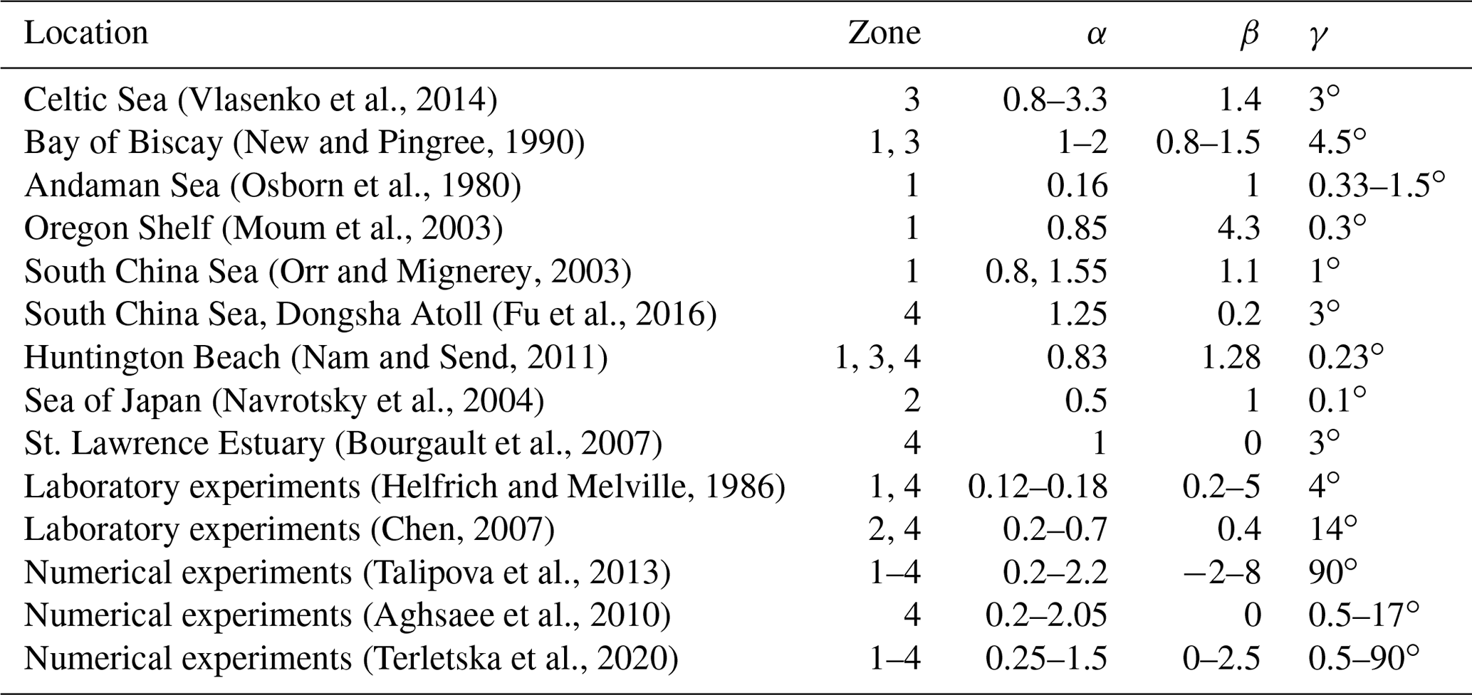
To compare the α β γ diagram with the data from field observations, the results of laboratory measurements and numerical simulations were analyzed by Terletska et al. (2020). They are presented in Table 1.
Terletska et al. (2020) showed that the results of field observations (Moum et al., 2003; Vlasenko et al., 2014; New and Pingree, 1990; Navrotsky et al., 2004; Osborn et al., 1980; Orr and Mignerey, 2003; Nam and Send, 2011; Fu et al., 2016), laboratory experiments (Helfrich and Melville, 1986; Cheng et al., 2011), and numerical experiments that simulate ISW transformation at laboratory scales (Talipova et al., 2013; Terletska et al., 2020) are in good agreement with the proposed classification. All data were identified as belonging to the corresponding diagram domain.
Let us consider the transformation of ISWs in the case of idealized topography and stratification that approximately follow the cross section in the Lufeng region in the SCS. The position of the cross section is shown in Fig. 1a. The data indicate (Ramp et al., 2010; Wang et al., 2013; Jackson, 2004) that internal waves from the Luzon Strait propagate westward to the Dongsha Atoll and then further to the Lufeng region and that the measured current in waves is about 1.5–2.0 m s−1. Wave amplitudes obtained using synthetic-aperture radar (SAR) images (during May after a strong thermocline developed in April) at a depth of about 300 m vary from 10 to 50 m with the depth of thermocline being about 40–65 m (Meng and Zhang, 2003). For numerical modeling of the idealized case that mimics the Lufeng region computational domain with a length L=18 km, a maximal depth m was considered (Fig. 1a). We approximated stratification in the Lufeng region using the two-layer density profile. The densities of the layers are ρ1 and ρ2 (depths h1 and h2, and ), and the pycnocline layer thickness is dh:
In numerical experiments, we vary the wave amplitudes (), m, m, and m, and we vary the slopes (γ), , , and . The slope inclination γ for a smooth curvilinear slope is measured as the maximal slope value. Corresponding values of α, β, and γ are given in Table 2. Density ρ1=1021.5 and ρ2=1025.5 (kg m−3), and the pycnocline layer thickness dh=15 m. The flux of salinity through the flume boundaries is also set to zero. The density profile from measurements from the SCS (May) (Orr and Mignerey, 2003) and the initial density profile (Eq. 7) are shown in Fig. 3. Depths layers are h1=50 m and h2=250 m for all runs.
Table 2ISW parameters from numerical experiments for the idealized Lufeng region in the SCS.
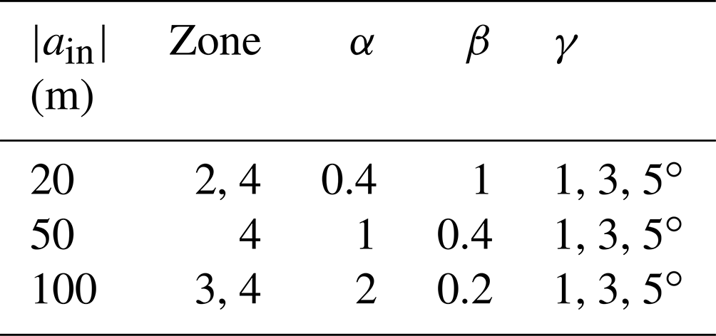
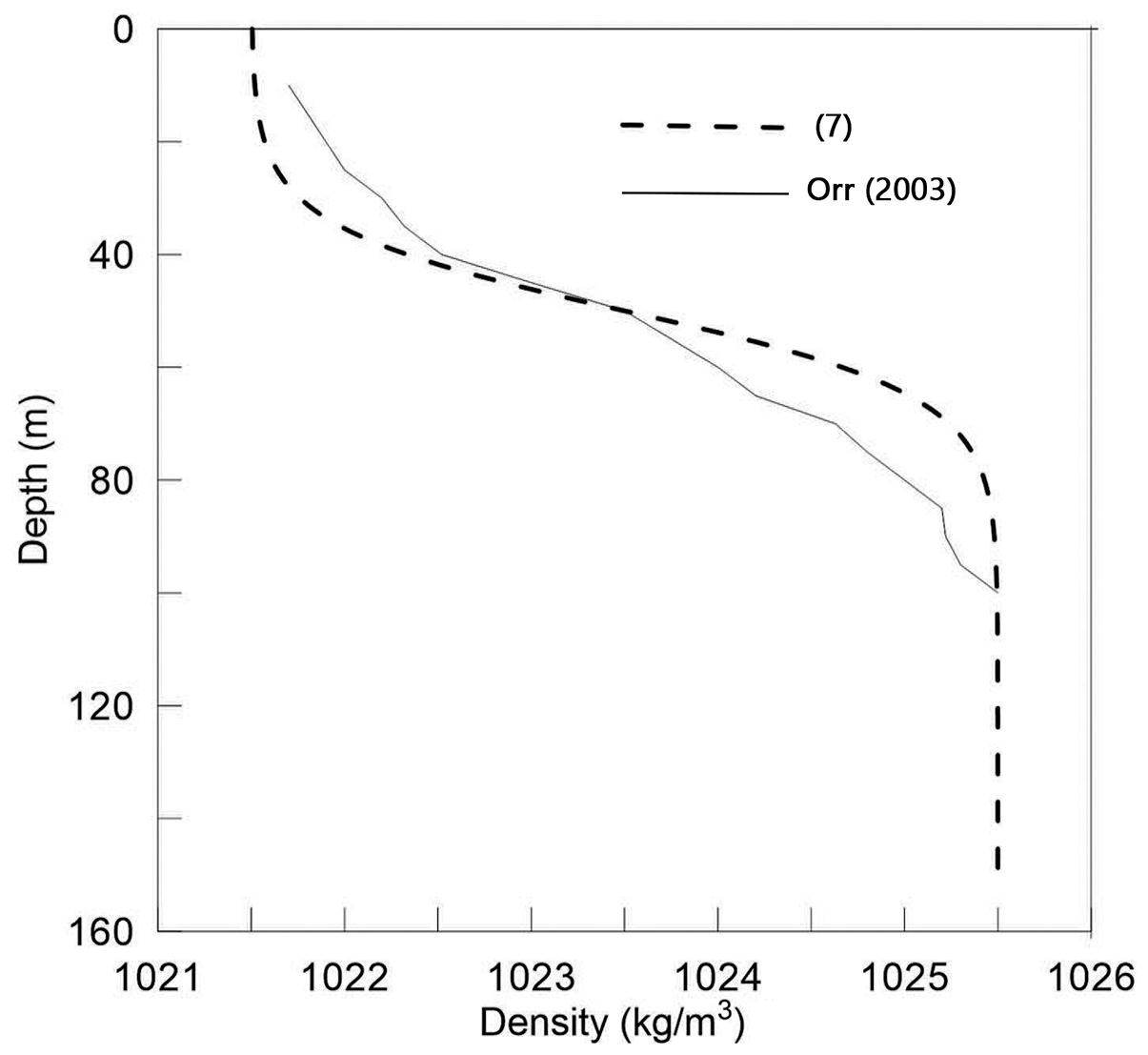
Figure 3Density profile from measurements from the SCS (May) (Orr and Mignerey, 2003), and the initial density profile (Eq. 7) used for numerical calculations.
The numerical simulations were carried out using a free-surface nonhydrostatic numerical model (Kanarska and Maderich, 2003; Maderich et al., 2012). The Smagorinsky model extended for stratified fluid (Siegel and Domaradzki, 1994) was used to explicitly describe the small-scale turbulent mixing and dissipation effects in the ocean-scale ISWs. In total, nine (three γ and three α) runs were carried out for all cases. The spatial resolution was m for all cases. A bottom-following sigma coordinate vertical system was used in the present model. A quasi-two-dimensional model with a resolution of 4 nodes across a wave tank with a resolution of 4200×250 nodes was used for the present calculations. No-slip boundary conditions were applied at the bottom and two end walls. Free-slip conditions were applied at the side walls. A mode-splitting technique and the decomposition of pressure and velocity fields on the hydrostatic and nonhydrostatic components were used in the numerical method; this is described in detail in Maderich et al. (2012).

Figure 4The evolution of an ISW with m in cross sections at times t=0, 60, 90, 120, 150, 160, 180, 210, 270 and 300 min (, α=1, β=0.4), respectively. xbr and xch.pol are the points of breaking and changing polarity, respectively.
The model was initialized using the iterative solution of the Dubreil-Jacotin–Long (DJL) (Dubreil-Jacotin, 1932) equation with the initial guess obtained from a weakly nonlinear theory. The “DJLES” spectral solver package (https://github.com/mdunphy/DJLES/, last access: 19 February 2018) in MATLAB was used. The transformation of an ISW with an initial amplitude of m is shown in Fig. 4. The minimum depth of the lower layer over the shelf is m, and the slope is . The parameters are α=1, β=0.4, and and correspond to the regime of breaking with changing polarity. The ISW propagation velocity is about 1.2 m s−1, which is typical for the Lufeng region in the SCS (Meng and Zhang, 2003). Using Eqs. (3) and (4), we could find the location on the slope where the ISW would change polarity ( m), and we found ISW breaking at the place where hbr≈40 m. It can be seen from Fig. 4 that ISW m first changes its polarity at time t=2 h 30 min and then breaks at the slope at t=2 h 40 min.
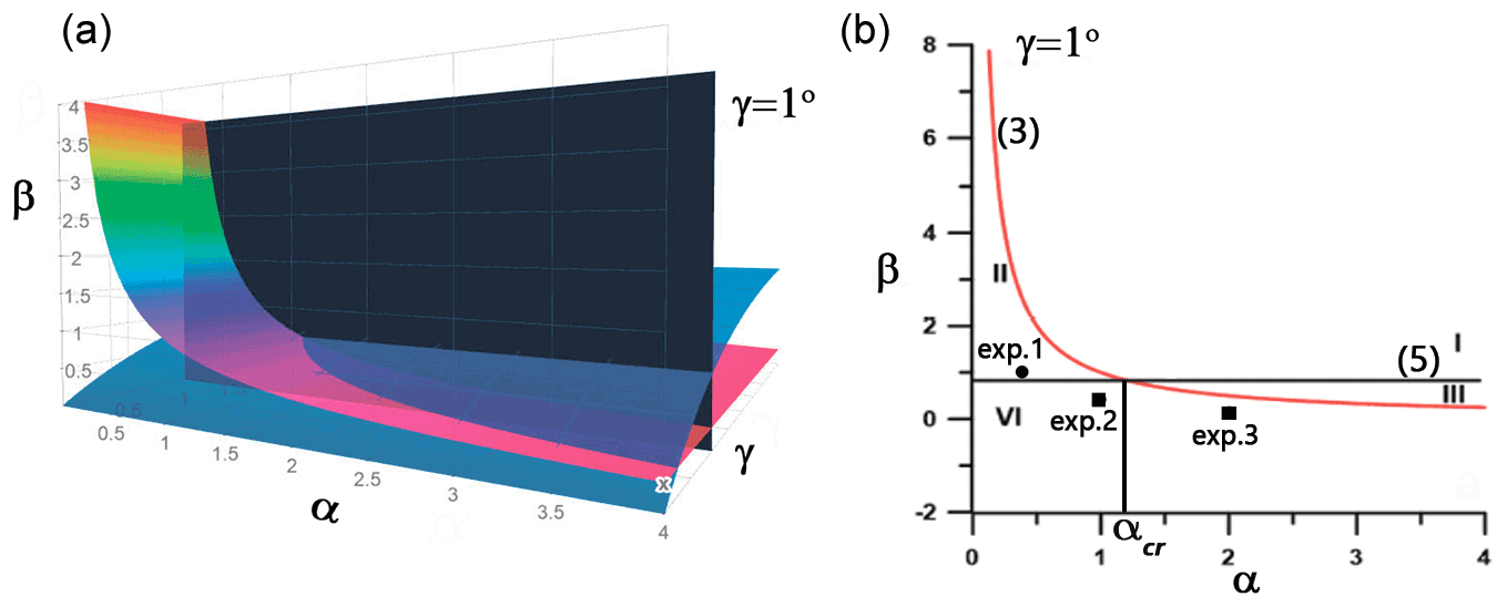
Figure 5(a) A three-dimensional diagram of regimes with the cross section αβ for . In panel (b), the red line corresponds to the polarity change criterion (3), and the black line corresponds to the breaking criterion (5); the circles represent cases of changing polarity but without wave breaking, and squares represent cases of changing polarity with wave breaking.
In Fig. 5a, a three-dimensional diagram of regimes with the cross section αβ for is shown. In Fig. 5b, the red line corresponds to the polarity change criterion (3), and the black line corresponds to the breaking criterion (5). Three experiments are also marked in panel (b): exp.1 – α=0.4, β=1, ; exp.2 – α=1, β=0.4, ; and exp.3 – α=2, β=0.2, . The first experiment, exp.1, represents cases of interaction of the ISW ( m) with polarity change but without wave breaking. The second experiment, exp.2, represents cases in which the ISW first changes its polarity from a depression- to an elevation-type wave and then breaks (Fig. 4). The final experiment, exp.3, represents cases in which the ISW breaks on the slope before it passes the changing polarity point.
An important characteristic of the wave–slope interaction is the loss of kinetic and available potential energy during the transformation. Energy transformation due to mixing leads to the transition of energy to background potential energy and then to energy dissipation. This can be estimated based on the budget of the wave energy before and after the transformation.
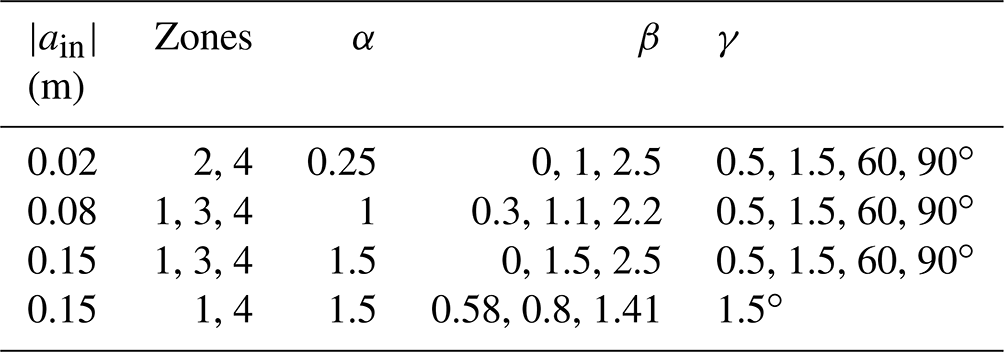
A calculation of energy dissipation was carried out for two configurations: (1) a real-scale experiment for the idealized Lufeng region in the SCS and (2) a laboratory-scale experiment with a trapezoid shelf-slope configuration (Terletska et al., 2020). The parameters of ISWs from the laboratory-scale numerical experiments by Terletska et al. (2020) are given in Table 3.
Table 3ISW parameters from laboratory-scale numerical experiments (Terletska et al., 2020).
The characteristics of the incoming and reflected wave were recorded in the cross sections xr, which are located near the foot of the slope, and the wave passing on the shelf was recorded in the cross section xl (Fig. 1b, c).
Energy loss from breaking waves was estimated following Lamb (2007) and Maderich et al. (2010) from the budget of depth-integrated pseudoenergy. To find the balance of the total energy, we have calculated the total energy of the incident, reflected, and transmitted waves before the slope and on the plateau using the depth-integrated pseudoenergy flux F(x,t):
where p is pressure disturbance due to a passing wave; U represents the horizontal velocities; and EPSE is the pseudoenergy density, which is the sum of the kinetic energy density Ek and the available potential density Ea (part of the potential energy available for conversion into kinetic energy). For the calculation of Ea, we used a reference density profile that was obtained by an adiabatic rearranging of the density field. Volume integration of these flows outside of the mixing zone then allows us to estimate the energy of the incoming PSEin waves, the reflected PSEref waves, and the transmitted PSEtr waves on the plateau.
where t1, t2, t3, t4, t5, and t6 are the time intervals at which incoming, reflected, and transmitted waves pass the given cross section.
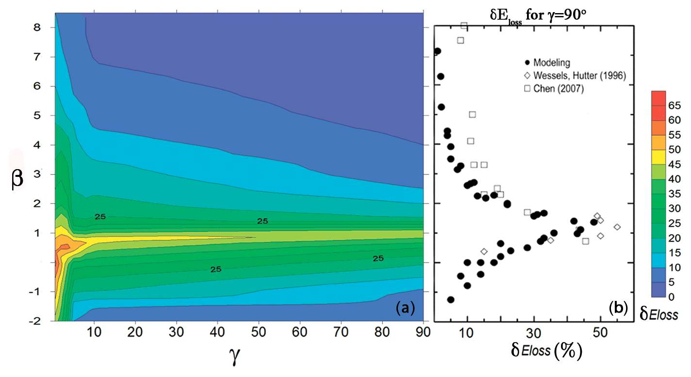
Figure 6(a) Energy loss (δEloss) from internal waves breaking on slopes for γ values from 0.5 to 90∘. (b) The limiting case, , corresponds to the numerical experiments by Talipova et al. (2013) and the results of laboratory experiments by Wessels and Hutter (1996) and Chen (2007) with steep obstacles.
The relative estimation of the energy loss (δEloss) is then given by
where PSEin is the pseudoenergy of the incident wave, and PSEtr and PSEref are the pseudoenergy of transmitted and incident waves, respectively. The energy loss from mixing during the interaction of the wave with the slope of δEloss (%) from the blocking parameter β is shown in Fig. 6a. This field of values, γβ, is built by 39 numerical experiments described in Table 3, 37 numerical experiments from Talipova et al. (2013) for , and 9 experiments from the present study. δEloss was estimated for a wide the range of slopes () and blocking parameters (). ISW energy loss for the limiting case of an underwater step when was compared with the results of laboratory experiments by Wessels and Hutter (1996) and Chen (2007) (Fig. 6b). It can be seen that wave transformation in Zone 4 is the most dissipative. With this type of transformation, energy losses reach up to 55 %. For slopes in the range of , the dependence of the energy dissipation on the blocking parameter β has almost the same pick shape as in the limiting case . For mild slopes of γ, we expect an increase in dissipation for all ranges of blocking parameter values of β.
We can compare the energy dissipation for a real-scale experiment with a laboratory-scale experiment with similar values of α and β and a slope of γ≈1. Considering cases with α=1 and β=0.4 for a slope of (real scale experiments in Table 2) and α=1 and β=0.3 for a slope of (laboratory-scale experiments in Table 3) (Zone 4 – wave breaking regime with polarity change), the difference is about 5 % ( % and %) for strong mixing.
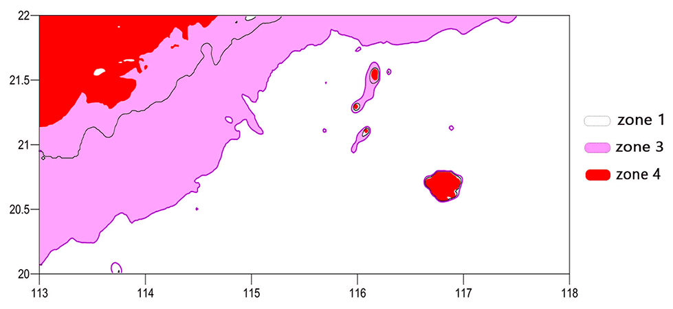
Figure 7Zone map for internal waves' transformation over the South China Sea shelf with an initial amplitude of 50 m and a depth of the mixed layer of 50 m.
To build a zone map for the shelf zone, the direction of the propagation of internal waves, the amplitude of incoming waves, and the stratification should be defined. These parameters could be found using the approach for estimating the geographic location of high-frequency nonlinear internal waves from Jackson et al. (2012), the amplitudes of the incoming internal waves, and the depth of the mixed layer. Figure 7 shows an example of a map with zones corresponding to the different regimes of interaction described above. These maps were constructed for the case of internal waves with an amplitude of ain=50 m and a mixed layer depth of h1=50 (Meng and Zhang, 2003). On this map, the black line is the 120 m isobath (shelf), the violet line is the polarity change curve h1=h2, and the red area is the zone of internal wave breaking (where ).
A three-dimensional α β γ classification diagram describing four types of ISW interaction with the slopes is discussed. Relations between the α, β, and γ parameters for each regime were obtained using the empirical relation for wave breaking conditions and weakly nonlinear theory for the criterion of the changing the polarity of the wave. The distinguished regimes are as follows: (1) the ISW propagates over a slope without changing polarity and wave breaking, (2) the ISW changes polarity over a slope without wave breaking, (3) the ISW breaks over a slope but without changing polarity, and (4) the ISW both breaks and changes polarity over a slope. The diagram is validated for realistic topography configurations. Numerical modeling of the idealized configuration that mimics the continental shelf in the Lufeng region (SCS) is carried out. The results of numerical experiments from the present study and from other laboratory experiments are in good agreement with the proposed classification and estimations. Based on present numerical experiments, internal solitary loss of wave energy from transformation over slope topography is estimated. We concluded that the results of field, laboratory, and numerical experiments are in good agreement with the proposed classification, which can be used for the identification of “hot spots” of energy dissipation in the ocean.
The output files for all of the numerical experiments reported in the paper are available from the corresponding author upon reasonable request.
KT and VM conceived the idea for the study; KT also carried out the numerical simulations, contributed to the design of figures, and participated in writing the paper. VM contributed to writing the paper and the interpretation of the results.
The contact author has declared that neither they nor their co-author has any competing interests.
Publisher’s note: Copernicus Publications remains neutral with regard to jurisdictional claims in published maps and institutional affiliations.
This article is part of the special issue “Nonlinear internal waves”. It is not associated with a conference.
This paper was edited by Zhenhua Xu and reviewed by two anonymous referees.
Aghsaee, P., Boegman, L., and Lamb, K. G.: Breaking of shoaling internal solitary waves, J. Fluid Mech., 659, 289–317, https://doi.org/10.1017/S002211201000248X, 2010. a, b
Alford, M. N., Peacok, T., Mackinnon, J. A., and Tang, D.: The formation and fate of internal waves in the South China Sea, Nature, 521, 65–69, 2015. a
Apel, J. R., Ostrovsky, L. A., and Stepanyants, Y. A.: Internal solitons in the ocean, J. Acoust. Soc. Am., 98, 2863, https://doi.org/10.1121/1.414338, 1995. a
Bai, X., Lamb, K., Xu, J., and Liu, Z.: On Tidal Modulation of the Evolution of Internal Solitary-Like Waves Passing Through a Critical Point, J. Phys. Oceanogr., 51, 2533–2552, https://doi.org/10.1175/JPO-D-20-0167.1, 2021. a
Boegman, L. and Stastna, M.: Sediment Resuspension and Transport by Internal Solitary Waves, Annu. Rev. Fluid Mech., 51, 129–154, https://doi.org/10.1146/annurev-fluid-122316-045049, 2019. a
Boegman, L., Ivey, G. N., and Imberger, J.: The degeneration of internal waves in lakes with sloping topography, Limnol. Oceanogr., 50, 1620–1637, https://doi.org/10.4319/lo.2005.50.5.1620, 2005. a
Bourgault, D., Blokhina, M. D., Mirshak, R., and Kelley, D. E.: Evolution of a shoaling internal solitary wavetrain, Geophys. Res. Lett., 34, L03601, https://doi.org/10.1029/2006GL028462, 2007. a
Chen, C.-Y.: An experimental study of stratified mixing caused by internal solitary waves in a two-layered fluid system over variable seabed topography, Ocean Eng., 34, 1995–2008, https://doi.org/10.1016/j.oceaneng.2007.02.014, 2007. a, b, c
Cheng, M. H., Hsu, J. R. C., and Chen, C. Y.: Laboratory experiments on waveform inversion of an internal solitary wave over a slope-shelf, Environ. Fluid Mech., 11, 353–384, 2011. a, b
Davis, K. A., Arthur, R. S., Reid, E. C., Rogers, J. S., Fringer, O. B., DeCarlo, T. M., and Cohen, A. L.: Fate of Internal Waves on a Shallow Shelf, J. Geophys. Res., 521, 65–69, https://doi.org/10.1029/2019JC015377, 2020. a
Dubreil-Jacotin, L.: Sur les ondes type permanent dans les liquides heterogenes, Atti R. Accad. Naz. Lincei, Mem. Cl. Sci. Fis., Mat. Nat., 15, 44–72, 1932. a
Fu, K.-H., Wang, Y.-H, Lee, C. P., and Lee, I. H.: The deformation of shoaling internal waves observed at the Dongsha Atoll in the northern South China Sea, Coast. Eng. J., 58, 1650001, 10.1142/S0578563416500017, 2016. a, b, c
Garrett, C. and Kunze, E.: Internal Tide Generation in the Deep Ocean, Annu. Rev. Fluid Mech., 39, 57–87, https://doi.org/10.1146/annurev.fluid.39.050905.110227, 2007. a
Gerkema, T. and Zimmerman, J. T. F.: Generation of Nonlinear Internal Tides and Solitary Waves, J. Phys. Oceanogr., 25, 1081–1094, https://doi.org/10.1175/1520-0485(1995)025<1081:GONITA>2.0.CO;2, 1995. a
Grimshaw, R., Pelinovsky, E., Talipova, T., and Kurkin, A.: Simulation of the transformation of internal solitary wave on oceanic shelves, J. Phys. Oceanogr., 34, 2774–2791, 2004. a
Helfrich, K. R. and Melville, W. K.: On long nonlinear internal waves over slope-shelf topography, J. Fluid Mech., 167, 285–308, 1986. a, b, c
Huang, X., Chen, Z., Zhao, W., Zhang, Z., Zhou, C., Yang, Q., and Tian, J.: An extreme internal solitary wave event observed in the northern South China Sea, Sci. Rep., 6, 30041, https://doi.org/10.1038/srep30041, 2016. a
Jackson, C. R.: An Atlas of Internal Solitary-like Waves and Their Properties, 2nd ed., Global Ocean Associates, Alexandria, VA, 560 pp., http://www.internalwaveatlas.com (last access: 26 May 2012), 2004. a, b
Jackson, C. R., da Silva, J. C. B., and Jeans, G.: The generation of nonlinear internal waves, Oceanography, 25, 108–123, 2012. a
Kanarska, Y. and Maderich, V.: A non-hydrostatic numerical model for calculating free-surface stratified flows, Ocean Dynam., 53, 176–185, 2003. a
Klymak, J. M., Pinkel, R., Liu, C. T., Liu, A. K., and David, L.: Prototypical solitons in the South China Sea, Geophys. Res. Lett., 33, L11607, https://doi.org/10.1029/2006GL025932, 2006. a
Klymak, J. M., Legg, S., and Pinkel, R.: A simple parameterization of turbulent tidal mixing near supercritical topography, J. Phys. Oceanogr., 40, 2059–2074, https://doi.org/10.1175/2010JPO4396.1, 2010. a, b
Kunze, E., MacKay, C., McPhee-Shaw, E. E., Morrice, K., Girton, J. B., and Terker, S. R.: Turbulent mixing and exchange with interior waters on sloping boundaries, J. Phys. Oceanogr., 42, 910–927, https://doi.org/10.1175/JPO-D-11-075.1, 2012. a
Lamb, K.: Energy and pseudoenergy flux in the internal wave field generated by tidal flow over topography, Cont. Shelf Res., 27, 1208–1232, https://doi.org/10.1016/j.csr.2007.01.020, 2007. a
Liu, A. K., Chang, S. Y., Hsu, M.-K., and Liang, N. K.: Evolution of nonlinear internal waves in the East and South China Seas, J. Geophys. Res., 103, 7995–8008, 1998. a, b
Maderich, V., Talipova, T., Grimshaw, R., Terletska, K., Brovchenko, I., Pelinovsky, E., and Choi, B. H.: Interaction of a large amplitude interfacial solitary wave of depression with a bottom step, Phys. Fluids, 22, 076602, https://doi.org/10.1063/1.3455984, 2010. a, b
Maderich, V., Brovchenko, I., Terletska, K., and Hutter, K.: Numerical simulations of the nonhydrostatic transformation of basin-scale internal gravity waves and wave-enhanced meromixis in lakes, chap. 4, in: Nonlinear internal waves in lakes, edited by: Hutter, K., Springer, Series: Advances in Geophysical and Environmental Mechanics, 193–276, https://doi.org/10.1007/978-3-642-23438-5_4, 2012. a, b
Maxworthy, T.: A note on the internal solitary waves produced by tidal flow over a three-dimensional ridge, J. Geophys. Res., 84, 338–346, https://doi.org/10.1029/JC084iC01p00338, 1979. a
Meng, J. and Zhang, J.: An Experiment of Internal Waves Observation by Synthetic Aperture Radar, P. ACRS, 1343–1345, https://scienceon.kisti.re.kr/srch/selectPORSrchArticle.do?cn=NPAP08058489 (last access: 10 December 2021), 2003. a, b, c
Moum, J. N., Farmer, D. M., Smyth, W. D., Armi, L., and Vagle, S.: Structure and generation of turbulence at interfaces strained by internal solitary waves propagating shoreward over the continental shelf, J. Phys. Oceanogr., 33, 2093–2112, 2003. a, b
Nakayama, K., Sato, T., Shimizu, K., and Boegman, L.: Classification of internal solitary wave breaking over a slope, Phys. Rev. Fluids, 4, 014801, https://doi.org/10.1103/PhysRevFluids.4.014801, 2019. a
Nam, S. H. and Send, U.: Direct evidence of deep water intrusions onto the continental shelf via surging internal tides, J. Geophys. Res., 116, C05004, https://doi.org/10.1029/2010JC006692, 2011. a, b, c
Navrotsky, V. V., Lozovatsky, I. D., Pavlova, E. P., and Fernando, H. J. S.: Observations of internal waves and thermocline splitting near a shelf break of the Sea of Japan (East Sea), Cont. Shelf Res., 24, 1375–1395, https://doi.org/10.1016/j.csr.2004.03.008, 2004. a, b
New, A. L. and Pingree, R. D.: Large amplitude internal soliton wave packets in the Bay of Biscay, Deep-Sea Res., 37, 513–524, 1990. a, b, c
Orr, M. H. and Mignerey, P. C.: Nonlinear internal waves in the South China Sea: observation of the conversion of depression internal waves to elevation internal waves, J. Geophys. Res., 108, 3064–2010, 2003. a, b, c, d, e, f
Osborn, A., Burch, T., Butman, B., and Pineda, J.: Internal solitons in the Andaman Sea, Science, 208, 451–460, https://doi.org/10.1126/science.208.4443.451, 1980. a, b, c
Pomar, L., Morsilli, M., Hallock, P., and Badenas, B.: Internal waves, an under-explored source of turbulence events in the sedimentary record, Earth-Sci. Rev., 111, 56–81, https://doi.org/10.1016/j.earscirev.2011.12.005, 2012. a
Ramp, S. R., Yang, Y. J., and Bahr, F. L.: Characterizing the nonlinear internal wave climate in the northeastern South China Sea, Nonlin. Processes Geophys., 17, 481–498, https://doi.org/10.5194/npg-17-481-2010, 2010. a, b
Sangrà, P., Basterretxea, G., Pelegrí, J. L., and Aristegui, J.: Chlorophyll increase due to internal waves in the shelf-break of Gran Canaria Island (Canary Islands), Sci. Mar., 65, 89–97, https://doi.org/10.3989/scimar.2001.65s189, 2001. a
Siegel, D. A. and Domaradzki, J. A.: Large-eddy simulation of decaying stably stratified turbulence, J. Phys. Oceanogr., 24, 2353–2386, 1994. a
St. Laurent, L. C., Garabato, A. C. N., Ledwell, J. R., Thurnherr, A. M., Toole, J. M., and Watson, A. J.: Turbulence and diapycnal mixing in Drake Passage, J. Phys. Oceanogr., 42, 2143–2152, https://doi.org/10.1175/JPO-D-12-027.1, 2012. a
Talipova, T., Terletska, K., Maderich, V., Brovchenko, I., Pelinovsky, E., Jung, K. T., and Grimshaw, R.: Solitary wave transformation on the underwater step: Asymptotic theory and numerical experiments, Phys. Fluids, 25, 032110, https://doi.org/10.1063/1.4797455, 2013. a, b, c, d, e
Terletska, K., Choi, B. H., Maderich, V., and Talipova, T.: Classification of internal waves shoaling over slope-shelf topography, Russian Journal of Earth Scienses, 20, ES4002, https://doi.org/10.2205/2020ES000730, 2020. a, b, c, d, e, f, g, h, i
Vlasenko, V., Stashchuk, N., Inall, M., and Hopkins, J. E.: Tidal energy conversion in a global hot spot: On the 3D dynamics of baroclinic tides at the Celtic Sea shelf break, J. Geophys. Res.-Oceans, 119, 3249–3265, 2014. a, b, c
Vlasenko, V. I. and Hutter, K.: Numerical experiments on the breaking of solitary internal waves over a slope shelf topography, J. Phys. Oceanogr., 32, 1779–1793, 2002. a, b
Wang, J., Huang, W., Yang, J., Zhang, H., and Zheng, G.: Study of the propagation direction of the internal waves in the South China Sea using satellite images, Acta Oceanol. Sin., 32, 42–50, https://doi.org/10.1007/s13131-013-0312-6, 2013. a, b
Wang, Y. H., Dai, C. F., and Chen, Y. Y.: Physical and ecological processes of internal waves on an isolated reef ecosystem in the South China Sea, Geophys. Res. Lett., 34, 1–7, 2007. a
Wessels, F. and Hutter, K.: Interaction of internal waves with a topographic sill in a two-layered fluid, J. Phys. Oceanogr., 26, 5–20, 1996. a, b, c
Zhang, X., Huang, X., Zhang, Z., Zhou, C., Tian, J., and Zhao, W.: Polarity Variations of Internal Solitary Waves over the Continental Shelf of the Northern South China Sea: Impacts of Seasonal Stratification, Mesoscale Eddies, and Internal Tides, J. Phys. Oceanogr., 48, 1349–1365, https://doi.org/10.1175/JPO-D-17-0069.1, 2018. a
- Abstract
- Introduction
- Regimes of ISW transformation over shelf-slope topography
- Data and methods
- Estimate of energy loss for internal waves breaking on slopes
- Conclusions
- Code and data availability
- Author contributions
- Competing interests
- Disclaimer
- Special issue statement
- Review statement
- References