Regional study of mode-2 internal solitary waves at the Pacific coast of Central America using marine seismic survey data

In this paper, a regional study of mode-2 internal solitary waves (ISWs) at the Pacific coast of Central America is carried out using the seismic reflection method. The observed relationship between the dimensionless propagation speed and the dimensionless amplitude (DA) of the mode-2 ISW is analyzed. When DA < 1.18, the dimensionless propagation speed seems to increase with increasing DA, divided into two parts with different growth rates. When DA > 1.18, the dimensionless propagation speed increases with increasing DA at a relatively small growth rate. We suggest that the influences of seawater depth (submarine topography), pycnocline depth, and pycnocline thickness on the propagation speed of the mode-2 ISW in the study area cause the relationship between dimensionless propagation speed and DA to diversify. The observed relationship between the dimensionless wavelength and the DA of the mode-2 ISW is also analyzed. When DA < 1, the nondimensional wavelengths seem to change from 2.5 to 7 for a fixed nondimensional amplitude. When DA > 1.87, the dimensionless wavelength increases with increasing DA. Additionally, the seawater depth has a great influence on the wavelength of the mode-2 ISW in the study area. Overall, the wavelength increases with increasing seawater depth. As for the vertical structure of the amplitude of the mode-2 ISW in the study area, we find that it is affected by the nonlinearity of the ISW and the pycnocline deviation (especially the downward pycnocline deviation).

1 Introduction

The amplitude and propagation speed of the mode-1 internal solitary wave (ISW) are larger than those of the mode-2 ISW. Mode-1 ISWs are more common in the ocean. In recent years, with the advancement of observation instruments, mode-2 ISWs in the ocean have been gradually observed, such as on the New Jersey shelf (Shroyer et al., 2010), in the South China Sea (Liu et al., 2013; Ramp et al., 2015; Yang et al., 2009), at Georges Bank (Bogucki et al., 2005), over the Mascarene Ridge in the Indian Ocean (Da Silva et al., 2011), and on the Australian North West Shelf (Rayson et al., 2019). Conventional physical oceanography observation and remote-sensing observation have their limitations: the horizontal resolution of conventional physical oceanography observation methods (such as mooring) is low and satellite remote sensing cannot see the ocean interior. Seismic oceanography (Holbrook et al., 2003; Ruddick et al., 2009; Song et al., 2021), as a new oceanography survey method, has high spatial resolution (vertical and horizontal resolution can reach about 10 m). It can better describe the spatial structure and related characteristics of mesoscale and small-scale phenomena in the ocean (Biescas et al., 2008, 2010; Fer et al., 2010; Holbrook and Fer, 2005; Holbrook et al., 2013; Pinheiro et al., 2010; Sallares et al., 2016; Sheen et al., 2009; Tsuji et al., 2005). Scholars have used the seismic oceanography method to carry out related studies on the geometry and kinematic characteristics (mainly related to propagation speed) of ISWs in the South China Sea, the Mediterranean Sea, and at the Pacific Coast of Central America (Bai et al., 2017; Fan et al., 2021a, b; Geng et al., 2019; Sun et al., 2019; Tang et al., 2014, 2018).

At present, research on the mode-2 ISW is mainly based on simulation. Through simulation, scholars have found that the pycnocline deviation affects the stability of the mode-2 ISW, and makes the top and bottom structure of the mode-2 ISW asymmetrical (Carr et al., 2015; Cheng et al., 2018; Olsthoorn et al., 2013). The instability caused by the pycnocline deviation mainly appears at the bottom of the mode-2 ISW. It manifests in the amplitude of the mode-2 ISW peak being smaller than the amplitude of the trough, because the upper sea layer is thinner than the bottom sea layer. The wave tail appears similar to a Kelvin–Helmholtz (KH) instability billow and the wave core appears as small-scale overturning motions (Carr et al., 2015; Cheng et al., 2018). Regarding the propagation speed of the mode-2 ISW, through simulation experiments, scholars found that it increases with increasing amplitude (Maxworthy, 1983; Salloum et al., 2012; Stamp and Jacka, 1995; Terez and Knio, 1998). Brandt and Shipley (2014) simulated the material transport of mode-2 ISWs with large amplitude in the laboratory. They found that when $\mathrm{2}a/h_{\mathrm{2}}>\mathrm{4}$ (a is the amplitude of the mode-2 ISW and h₂ is the pycnocline thickness; we define the dimensionless amplitude $\stackrel{\mathrm{̃}}{a}=\mathrm{2}a/h_{\mathrm{2}}$ for the convenience of using in the following text), the linear relationship between propagation speed (wavelength) and amplitude is destroyed, i.e., when the amplitude $\stackrel{\mathrm{̃}}{a}$ ≥ 4, the propagation speed increases relatively slowly and the wavelength increases rapidly. The authors believe that the above results are caused by strong internal circulation related to the very large amplitude and the influence of the top and bottom boundaries. Chen et al. (2014) calculated the Korteweg–de Vries (KdV) propagation speed and the fully nonlinear propagation speed of the ISW as a function of the pycnocline depth and the pycnocline thickness, respectively. They found that the propagation speed of the mode-2 ISW increases monotonously with increasing pycnocline depth, first increasing and then decreasing with the increasing pycnocline thickness. Carr et al. (2015) found by simulations that the pycnocline deviation has little effect on the propagation speed, wavelength, and amplitude of the mode-2 ISW. Maderich et al. (2015) found that for mode-2 ISWs, when the dimensionless amplitude $\stackrel{\mathrm{̃}}{a}<\mathrm{1}$, the deep-water weakly nonlinear theory (Benjamin, 1967) can describe the numerical simulation and experimental simulation results well. When $\stackrel{\mathrm{̃}}{a}>\mathrm{1}$, the wavelength (propagation speed) increases with the amplitude faster than the results predicted by the deep-water weakly nonlinear theory. However, the solution of Kozlov and Makarov (1990) can estimate the corresponding wavelength and propagation speed when the amplitude is $\mathrm{1}<\stackrel{\mathrm{̃}}{a}<\mathrm{5}$ well. Terletska et al. (2016) found that the propagation speed and amplitude of the mode-2 ISW decreases after passing the step. Moreover, the closer the mode-2 ISW is to the step in the vertical direction at the time of incidence, the smaller the propagation speed and amplitude of the mode-2 ISW are after passing the step. Kurkina et al. (2017) used the Generalized Digital Environmental Model (GDEM) to find that seawater depth in the South China Sea is the main controlling factor of the mode-2 ISW propagation speed, and that the propagation speed increases exponentially with increasing seawater depth. Deepwell et al. (2019) found by simulation that the relationship between the mode-2 ISW propagation speed and amplitude has a strong quadratic trend. They speculated that this quadratic relationship comes from the influence of seawater depth (at a smaller seawater depth, the propagation speed is also lower).

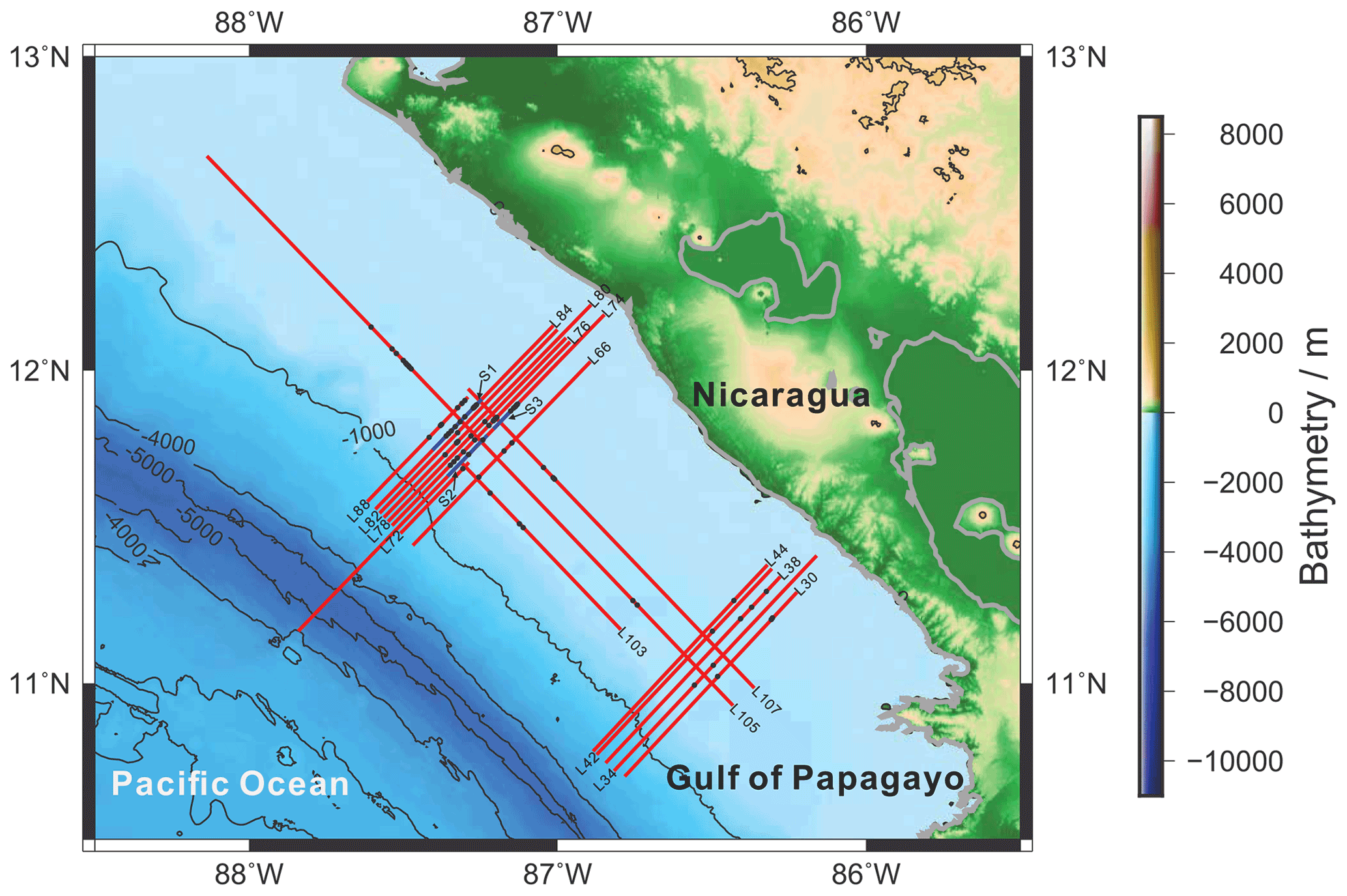
Figure 1 Distribution of multichannel seismic data. The red lines indicate the positions of the survey lines, and the black filled circles on the red lines indicate the positions of the observed mode-2 ISWs. The blue lines S1, S2, and S3 are part of the seismic sections containing the mode-2 ISWs, which will be displayed in Figs. 3 and 4.

The simulation can reveal the kinematic characteristics of the mode-2 ISW well. However, the actual ocean conditions are often more complicated, which is manifested in the diversity of controlling factors in the kinematic process. The observations, including the seismic oceanography method, are also required to continually provide a basic understanding of the geometry and kinematic characteristics of the mode-2 ISW. For example, limited by factors such as lower spatial resolution of the observation methods, previous scholars have performed less direct observational research on the propagation speed and wavelength of the mode-2 ISW in the ocean. Furthermore, there is even less research (including observational research) on the vertical structure of the mode-2 ISW. The seismic oceanography method has advantages for carrying out the abovementioned research, due to its higher spatial resolution. The Pacific coast of Central America (western Nicaragua) has relatively continuous submarine topography along the coastline, including the continental shelf and continental slope, with a seawater depth of 100–2000 m (Fig. 1). At present, there is relatively little research work available on internal waves in this area. We reprocessed the historical seismic data in this area and identified a large number of mode-2 ISWs with relatively complete spatial structures in the region. This discovery is very helpful for carrying out observational research on the geometry and kinematic characteristics of mode-2 ISWs. Fan et al. (2021a, b) used the multichannel seismic data of the survey lines L88 and L76 (cruise EW0412; see Fig. 1 for the survey line locations) on the Pacific coast of Central America to report the mode-2 ISWs in this area and study their shoaling features of the mode-2 ISW in this area, respectively. However, a single survey line can only reveal the local characteristics of the mode-2 ISW in the study area. A in-depth understanding of the geometry and kinematic characteristics (mainly related to propagation speed) of the mode-2 ISW in the study area requires a regional systematic study. In this work, we reprocessed the seismic data of the entire study area and identified numerous mode-2 ISWs on multiple survey lines in the region (the positions of the observed ISWs and the survey lines they located to are shown by the black filled circles and the red lines in Fig. 1, respectively). Based on the numerous mode-2 ISWs observed by multiple survey lines in the study area, this paper will conduct a regional study on the characteristic parameters. These characteristic parameters include the pycnocline deviation degree, propagation speed, and wavelength of the mode-2 ISW, as well as the vertical structure characteristics of the mode-2 ISW amplitude in the study area.

2 Data and methods

This paper mainly uses seismic reflection to conduct a regional study on the mode-2 ISWs at the Pacific coast of Central America. The seismic data of the cruise EW0412 used in this study were provided by the Marine Geoscience Data System (MGDS; http://www.marine-geo.org/, last access: 30 March 2022). The cruise EW0412 collected high-resolution multichannel seismic data from the continental shelf to the continental slope in the coastal areas of the Sandino Forearc Basin, Costa Rica, Nicaragua, Honduras, and El Salvador (Fulthorpe and McIntosh, 2014). The seismic acquisition parameters of the cruise EW0412 are as follows: the sampling interval is 1 ms, each shot gather has 168 traces, the shot interval is 12.5 m, the trace interval is 12.5 m, and the minimum offset is 16.65 m. The seawater seismic reflection sections used in this study were obtained through the following processing processes: defining geometry, noise attenuation, common midpoint (CMP) sorting, velocity analysis, normal moveout (NMO), stacking, and post-stack denoising. Previous studies have demonstrated that seismic reflections generally track isopycnal surfaces (Holbrok et al., 2013; Krahmann et al., 2009; Sheen et al., 2011). We believe that the seismic stacked sections (e.g., Figs. 3 and 4) include the information on density profile. Therefore, we do not provide plots of the density profile upon which the waves propagate (even in schematic form) in the following sections.

In this research, we try to use the maximum amplitude (the maximum vertical displacement of isopycnals) to study the amplitude-related characteristics of mode-2 ISWs, such as the relationship between propagation speed and maximum amplitude in Fig. 9. However, the correlativity is not very strong. We also noticed that the amplitude, defined as the maximum vertical displacement of isopycnals, is used less for quantitatively describing the amplitude-related characteristics of mode-2 ISWs. Particularly, in mode-2 ISW simulation research, scholars often use the dimensionless amplitude $\stackrel{\mathrm{̃}}{a}$ to quantitatively describe the amplitude-related characteristics of mode-2 ISWs, like the relationship between propagation speed and dimensionless amplitude (Brandt and Shipley, 2014; Carr et al., 2015). It is important to point out that in mode-2 ISW simulation research, the dimensionless amplitude used comes from the three-layer model. However, the mode-2 ISW in the actual ocean has a multilayer structure (multiple continuous density displacements above and below the mid-depth of the pycnocline). It is different from the three-layer model used in the simulation experiment to describe the convex mode-2 ISW. As for the three-layer model, the upper layer of the convex mode-2 ISW is the peak and the lower layer is the trough. Because there is almost no work from the previous scholars to define the mode-2 ISW dimensionless amplitude based on the mode-2 ISW in the actual ocean, we attempt to build an equivalent three-layer model to compare our observational results with the simulation results and to quantitatively describe the amplitude-related characteristics of mode-2 ISWs. The equivalent three-layer model results from the mode-2 ISW with a continuous structure in the actual ocean. It should be pointed that the equivalent three-layer model is defined by attempting to analogize with the three-layer model. Therefore, it is not identical to the three-layer model as shown in Fig. 1 in Brandt and Shipley (2014). We use the equivalent three-layer model to calculate the equivalent amplitude, the equivalent pycnocline thickness, and the equivalent wavelength of the mode-2 ISW. Similarly, as the equivalent three-layer model is defined by seeking to analogize with the three-layer model, the equivalent amplitude (dimensionless amplitude) is not completely equivalent to that used by Brandt and Shipley (2014). For the mode-2 ISW with a multilayer structure, the sum of all ISW peak amplitudes a_p and the sum of all ISW trough amplitudes a_t are taken as the equivalent peak and trough amplitudes, respectively, of the mode-2 ISW with a three-layer model structure. The equivalent amplitude of the mode-2 ISW with a three-layer model structure is then the average of a_p and a_t. The equivalent pycnocline thickness is calculated by $h_{\mathrm{2}}=h-a_{\mathrm{p}}-a_{\mathrm{t}}$, where h is the seawater thickness affected by the mode-2 ISW with a multilayer structure. The equivalent wavelength of the mode-2 ISW with a three-layer model structure is the average of all ISW peak and trough wavelengths in the multilayer structure. The detailed calculation process is described in Fan et al. (2021a). This study uses an improved ISW apparent propagation speed calculation method to calculate the apparent propagation speed of ISW. This method firstly performs pre-stack migration of the common-offset gather sections, and then picks the CMP and shotpoint pairs corresponding to the ISW trough or peak from the pre-stack migration sections of different offsets with a high signal-to-noise ratio. By fitting the CMP–shotpoint pairs, we can calculate the apparent propagation speed and apparent propagation direction of the ISW. The ISW horizontal velocity can be expressed by the equation as follows:

$$\begin{array}{}\text{(1)}& v={\displaystyle \frac{\mathrm{cmp}\mathrm{2}-\mathrm{cmp}\mathrm{1}}{T}}={\displaystyle \frac{\mathrm{cmp}\mathrm{2}-\mathrm{cmp}\mathrm{1}}{(s\mathrm{2}-s\mathrm{1})\mathrm{d}t}},\end{array}$$

where cmp1 and cmp2​​​​​​​ are the peak or trough positions of the ISW at different times, s1 and s2 are the shot numbers corresponding to cmp1 and cmp2, and dt is the time interval of shots. The detailed calculation process is described in Fan et al. (2021a).

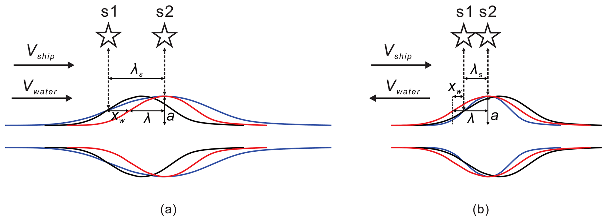
Figure 2 Schematic diagram of the apparent wavelength correction of the mode-2 ISW. (a) The ISW moves in the same direction as the ship. (b) The ISW moves in the opposite direction to the ship. S1 denotes the self-excitation and self-reception position of the ship at $\mathrm{1}/\mathrm{2}$ amplitude of the ISW at the beginning. S2 denotes the self-excitation and self-reception position of the ship at the peak of the amplitude of the ISW. V_ship is the ship speed and V_water is the ISW propagation speed, λ_s is the apparent wavelength of the ISW observed by the seismic stacked section, λ is the actual wavelength of the ISW, a is the amplitude of the ISW, and x_w is the distance moved by the ISW during the time the ship moves from S1 to S2. The black curve denotes the ISW at the beginning. The red curve denotes the ISW moved x_w distance from the starting position. The blue curve denotes the ISW observed on the seismic stacked section.

The wavelength of the mode-2 ISW is usually defined as the half-width at half-amplitude of the ISW (Carr et al., 2015; Stamp and Jacka, 1995), as shown by λ in Fig. 2. In a seismic survey, the sound is sent from a towed source, reflected from aquatic structures, and received by an array of towed hydrophones with time delays that depends on the geometry of the ray paths taken. A detailed introduction to seismic principles is provided by Ruddick et al. (2009). Traditional seismic reflection imaging assumes that the underground structure is fixed. Since mode-2 ISWs move relatively fast in the horizontal direction (about 0.5 m s⁻¹) during the seismic acquisition process, seismic reflection imaging of mode-2 ISWs needs to consider the influence of the horizontal motion of the ISW. The wavelength of the mode-2 ISW observed by the seismic reflection method is the apparent wavelength. The apparent wavelength of the mode-2 ISW is controlled by the relative motion direction of the ship and the ISW, the ship speed, and the propagation speed of the ISW. The propagation speed of the mode-2 ISW (about 0.5 m s⁻¹) is generally lower than the ship speed (about 2.5 m s⁻¹) during seismic acquisition. When correcting the apparent wavelength of the mode-2 ISW to obtain the actual wavelength, one distinguishes between two situations: the situation in which the motion direction of the ISW and the ship are the same, and the situation in which these are opposite to each other, as shown in Fig. 2. When the ISW and the ship move in the same direction, the wavelength (apparent wavelength) estimated from the seismic stacked section is larger, i.e., the wavelength (apparent wavelength λ_s) of the ISW observed on the seismic stacked section denoted by the blue curve in Fig. 2a is greater than the wavelength λ of the actual ISW at the beginning and end, denoted by the black and red curves in Fig. 2a, respectively. The influence of the horizontal movement of the ISW should be eliminated. When correcting the apparent wavelength λ_s to obtain the actual wavelength λ, it is necessary to subtract the distance x_w moved by the ISW within the seismic acquisition time corresponding to the apparent wavelength distance of the ISW, i.e.,

$$\begin{array}{}\text{(2)}& \mathit{\lambda }={\mathit{\lambda }}_{\mathrm{s}}-x_{\mathrm{w}}={\mathit{\lambda }}_{\mathrm{s}}-{\displaystyle \frac{{\mathit{\lambda }}_{\mathrm{s}}}{V_{\mathrm{ship}}}}{V}_{\mathrm{water}},\end{array}$$

where V_ship is the ship speed, and V_water is the propagation speed of the ISW (Fig. 2a).

When the ISW and the ship move in opposite directions, the wavelength (apparent wavelength) estimated from the seismic stacked section is smaller, i.e., the wavelength (apparent wavelength λ_s) of the ISW observed on the seismic stacked section denoted by the blue curve in Fig. 2b is smaller than the wavelength λ of the actual ISW at the beginning and end, denoted by the black and red curves in Fig. 2b, respectively. The influence of the horizontal movement of the ISW should be eliminated. When correcting the apparent wavelength λ_s to obtain the actual wavelength λ, it is necessary to add the distance x_w moved by the ISW within the seismic acquisition time corresponding to the apparent wavelength distance of the ISW, i.e.,

$$\begin{array}{}\text{(3)}& \mathit{\lambda }={\mathit{\lambda }}_{\mathrm{s}}+x_{\mathrm{w}}={\mathit{\lambda }}_{\mathrm{s}}+{\displaystyle \frac{{\mathit{\lambda }}_{\mathrm{s}}}{V_{\mathrm{ship}}}}{V}_{\mathrm{water}},\end{array}$$

where V_ship is the ship speed, and V_water is the propagation speed of the ISW (Fig. 2b).

3 Results and interpretations

3.1 Typical sections interpretation and regional distribution characteristics of the mode-2 ISW

In addition to the survey lines L88 and L76 with mode-2 ISWs observed by Fan et al. (2021a, b), we also found mode-2 ISWs on many other survey lines in the study area. Two typical survey lines are L84 and L74 (see the red lines in Fig. 1 for the locations of these two survey lines). Figure 3 shows the partial seismic stacked section S1 of the survey line L84 (see the blue line in Fig. 1 for the location of section S1). We have identified 10 mode-2 ISWs from the seismic section S1 (see Fig. 3 for their positions and corresponding numbers. ISW1–ISW4 are located at the shelf break and ISW5–ISW10 are located on the continental shelf) and calculated their characteristic parameters such as seafloor depth (seawater depth) H, maximum amplitude (in the vertical direction), equivalent amplitude a, equivalent pycnocline thickness h₂, dimensionless amplitude $\stackrel{\mathrm{̃}}{a}$, mid-depths of the pycnocline h_c, the degree to which the mid-depth of the pycnocline deviates from $\mathrm{1}/\mathrm{2}$ seafloor depth P_d, equivalent wavelength λ, dimensionless wavelength (we define the dimensionless wavelength ${\mathit{\lambda }}_{\mathrm{0}}=\mathrm{2}\mathit{\lambda }/h_{\mathrm{2}}$ for the convenience of using in the following text), and apparent propagation speed U_c (Table 1). The equivalent wavelength and the dimensionless wavelength in Table 1 have been corrected using Eq. (2) as the ISWs have the same motion direction as the ship, and the ISWs with the large propagation speed estimation error have been corrected using a propagation speed of 0.5 m s⁻¹. The maximum amplitudes of the ISWs ISW1–ISW7 on survey line L84 are all less than 10 m and the maximum amplitudes of ISW8–ISW10 are larger, around 15 m. The $\stackrel{\mathrm{̃}}{a}$ values ($\stackrel{\mathrm{̃}}{a}=\mathrm{2}a/h_{\mathrm{2}}$) of these 10 mode-2 ISWs on the survey line L84 are all less than 2 (Table 1). We define an ISW whose $\stackrel{\mathrm{̃}}{a}$ value is less than 2 as a mode-2 ISW with a small amplitude and an ISW whose $\stackrel{\mathrm{̃}}{a}$ value is larger than 2 as a mode-2 ISW with a large amplitude. The 10 mode-2 ISWs on the survey line L84 belong to the mode-2 ISWs with small amplitude. The $\stackrel{\mathrm{̃}}{a}$ values of ISW8, ISW9, and ISW10 are around 1; their amplitudes are relatively large compared to the other small-amplitude mode-2 ISWs. When calculating the P_d values, we find that the pycnocline centers of ISW8, ISW9, and ISW10 are deeper than $\mathrm{1}/\mathrm{2}$ seafloor depths, whereas the pycnocline centers of the other seven mode-2 ISWs are shallower than $\mathrm{1}/\mathrm{2}$ seafloor depths (Table 1). For ISW1, ISW2, and ISW3, the P_d values are greater than 20 %, which appears as asymmetry of the waveforms (the asymmetry of the front and rear waveform, and the asymmetry of the top and bottom waveform). When the P_d value is small, the waveform of the mode-2 ISW is more symmetrical, such as in ISW8, ISW9, and ISW10. The waveforms of ISW1, ISW2, and ISW3 at the shelf break are asymmetrical and their dimensionless wavelengths λ₀ (${\mathit{\lambda }}_{\mathrm{0}}=\mathrm{2}\mathit{\lambda }/h_{\mathrm{2}}$) are significantly larger than the λ₀ values of the ISWs on the continental shelf which have the same level of dimensionless amplitudes ($\stackrel{\mathrm{̃}}{a}$), for example, the $\stackrel{\mathrm{̃}}{a}$ value of ISW2 is 0.45 and the value of λ₀ is 9.55; the value of $\stackrel{\mathrm{̃}}{a}$ of ISW7 is 0.42 and the value of λ₀ is 3.49). It means that the overall relationship between dimensionless wavelength λ₀ and the dimensionless amplitude $\stackrel{\mathrm{̃}}{a}$ is not an absolutely linear correlation (the λ₀ increases with the increasing $\stackrel{\mathrm{̃}}{a}$). The apparent propagation speeds U_c of the 10 mode-2 ISWs on the survey line L84 are about 0.5 m s⁻¹ and the apparent propagation directions are all shoreward. For ISWs with small apparent propagation speed calculation errors in shallow water (ISW6, ISW7, and ISW9), the U_c does not strictly increase with increasing $\stackrel{\mathrm{̃}}{a}$. For example, the $\stackrel{\mathrm{̃}}{a}$ value of ISW6 is 0.4 and the U_c value is about 0.58 m s⁻¹, and the $\stackrel{\mathrm{̃}}{a}$ value of ISW9 is 1.19 and the U_c value is about 0.38 m s⁻¹.

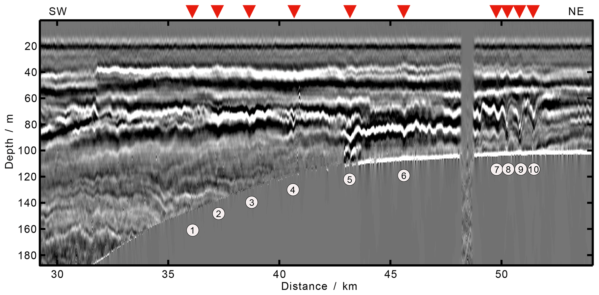
Figure 3 Seismic stacked section S1, with observed mode-2 ISWs on the survey line L84. Arrows and numbers indicate the 10 identified mode-2 ISWs ISW1–ISW10. The location of the S1 seismic stacked section is shown in Fig. 1. The horizontal axis indicates the distance to the starting point of survey line L84. The survey line L84 acquisition time was from 07:15:14 GMT on 17 December 2004 to 17:26:49 GMT on 17 December 2004.

Table 1 Characteristic parameters of the 10 mode-2 internal solitary waves in Survey Line L84.

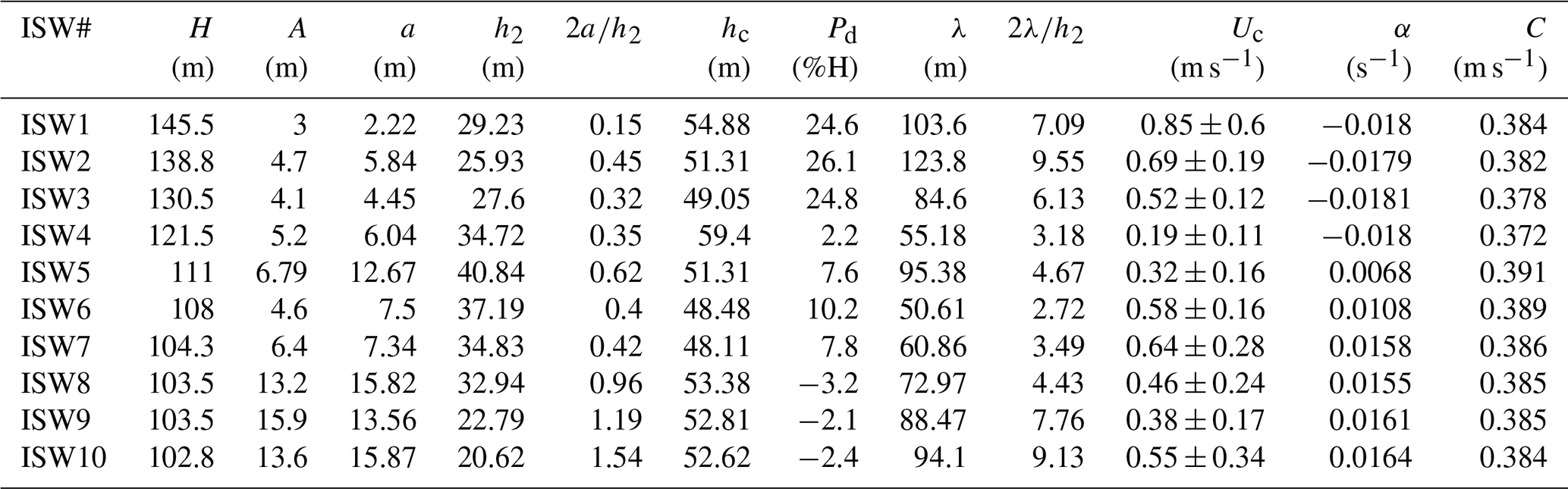
Note. H, seafloor depths; A, maximum amplitudes; a, equivalent ISW amplitudes; h₂, equivalent pycnocline thicknesses; h_c, the mid-depths of the pycnocline; P_d, the degree to which the mid-depth of the pycnocline deviates from $\mathrm{1}/\mathrm{2}$ seafloor depth; λ, equivalent wavelengths; U_c, apparent propagation speeds obtained from seismic observation; α, quadratic nonlinear coefficient shown in Eq. (9) and obtained by solving Eq. (6); C, linear phase speed which is obtained by solving Eq. (6).

Figure 4 Panels (a) and (b) are the seismic stacked sections S2 and S3, respectively, with observed mode-2 ISWs on the survey line L74. The arrows and the numbers indicate the seven identified mode-2 ISWs ISW11–ISW17. The locations of the seismic stack section S2 and S3 are shown in Fig. 1. The horizontal axis indicates the distance to the starting point of survey line L74. The survey line 74 acquisition time was from 06:31:03 GMT on 3 December 2004 to 02:30:01 GMT on 4 December 2004.

Table 2 Characteristic parameters of the seven mode-2 internal solitary waves in survey line L74.

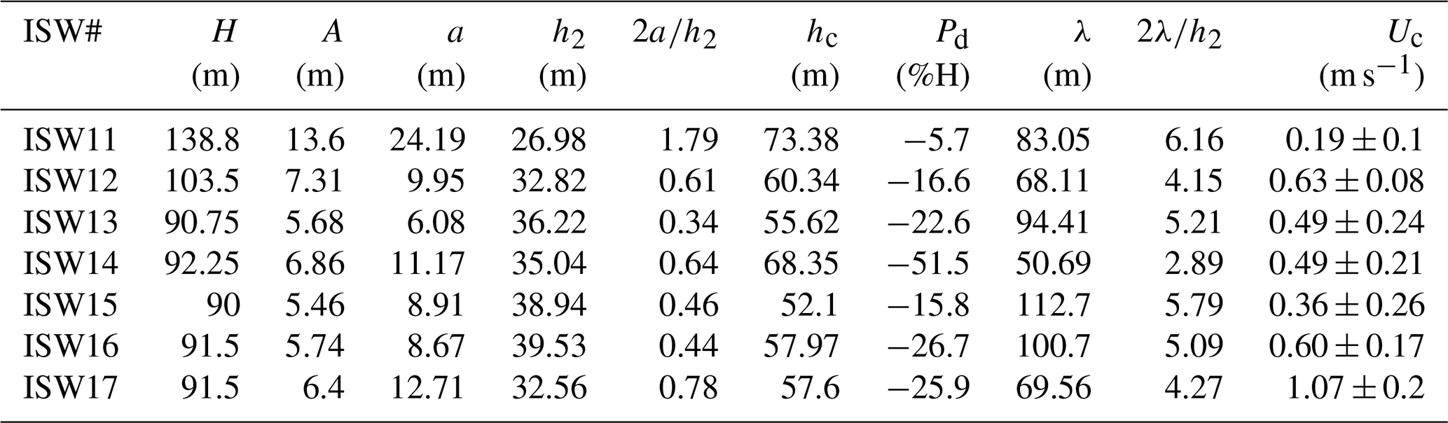
Note. H  seafloor depths; A, maximum amplitudes; a, equivalent ISW amplitudes; h₂, equivalent pycnocline thicknesses; h_c, the mid-depths of the pycnocline; P_d, the degree to which the mid-depth of the pycnocline deviates from $\mathrm{1}/\mathrm{2}$ seafloor depth; λ, equivalent wavelengths; U_c, apparent propagation speeds obtained from seismic observation.

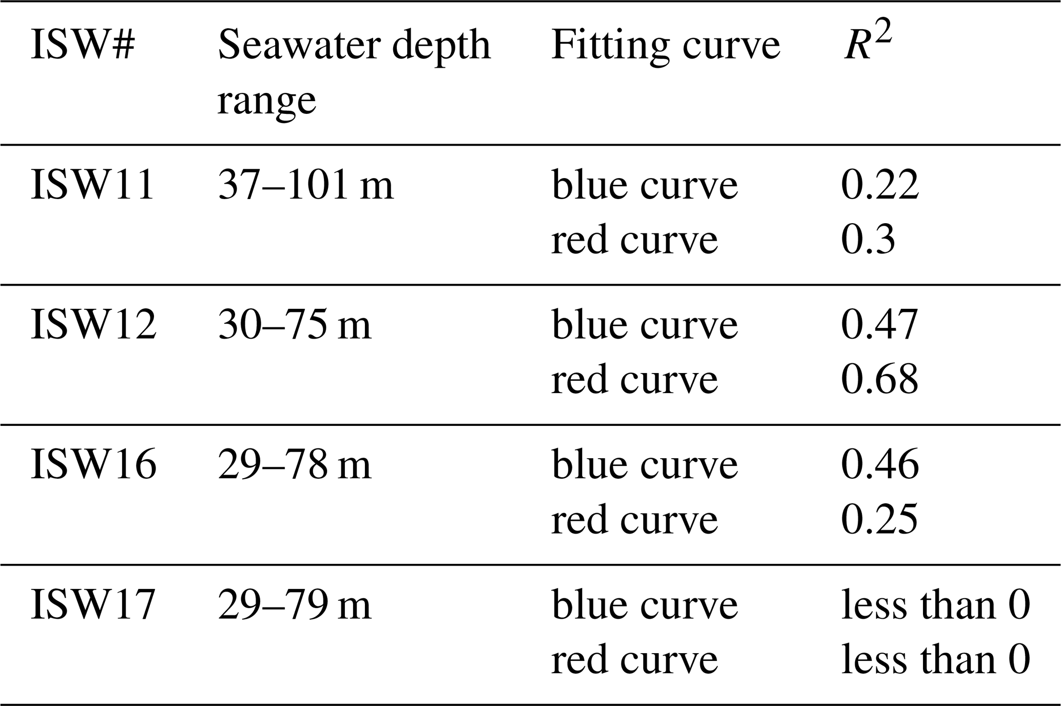
Survey line L74 is located southeast of survey line L84 (see Fig. 1 for the specific location). Figure 4 shows the partial seismic stacked sections (S2 and S3) of survey line L74. We have identified seven mode-2 ISWs from the seismic sections S2 and S3. Their positions and corresponding numbers are shown in Fig. 4 and the characteristic statistical parameters are shown in Table 2. The equivalent wavelength and the dimensionless wavelength in Table 2 have been corrected using Eq. (2) as the ISWs have the same motion direction as the ship, and the ISWs with the large propagation speed estimation error have been corrected using a propagation speed of 0.5 m s⁻¹. The maximum amplitudes of the ISWs ISW12–ISW17 on the survey line L74 are all less than 10 m, whereas the maximum amplitude of ISW11 is larger, 13.6 m. The $\stackrel{\mathrm{̃}}{a}$ values of these seven mode-2 ISWs are all less than 2 (Table 2); they are the mode-2 ISWs with small amplitude. Among them, the amplitude of ISW11 is slightly larger. When calculating the P_d value, we find that the pycnocline centers of the mode-2 ISWs ISW11–ISW17 are all deeper than $\mathrm{1}/\mathrm{2}$ of the seafloor depths (Table 2). Except for ISW11 (the bottom reflection event is broken), for the other six mode-2 ISWs ISW12–ISW17, the P_d values are greater than 15 %. The asymmetry of ISW12 and ISW13 is manifested in that the connection between the top peaks of the ISW and the bottom troughs of the ISW is not vertical. The pycnocline center of ISW14 deviates from $\mathrm{1}/\mathrm{2}$ of the seafloor depth the most, by 51.5 %. Its asymmetry is manifested in the large difference between the top and bottom waveforms near the pycnocline center. ISW15, ISW16, and ISW17 are located on the continental shelf, and their pycnocline deviations are larger. However, their waveforms are more symmetrical than other ISWs. When the downward pycnocline deviation is large, the influence of pycnocline deviation on the stability of the mode-2 ISW is more complicated than when the pycnocline deviates upwards, and may be controlled by factors such as wavelength. There is no absolute linear correlation relationship between the dimensionless wavelengths λ₀ and the dimensionless amplitudes $\stackrel{\mathrm{̃}}{a}$ of the seven mode-2 ISWs on survey line L74 (the λ₀ increases with the increasing $\stackrel{\mathrm{̃}}{a}$). For example, the $\stackrel{\mathrm{̃}}{a}$ values of ISW12 and ISW14 are greater than that of ISW16, but the λ₀ value of ISW16 is greater than the λ₀ values of ISW12 and ISW14. The apparent propagation speeds U_c of the seven mode-2 ISWs on survey line L74 are about 0.5 m s⁻¹ and their propagation directions are all shoreward. For the ISWs in shallow water whose apparent propagation speed calculation errors are small (ISW12, ISW14, ISW16, and ISW17), the U_c value generally increases with increasing $\stackrel{\mathrm{̃}}{a}$.

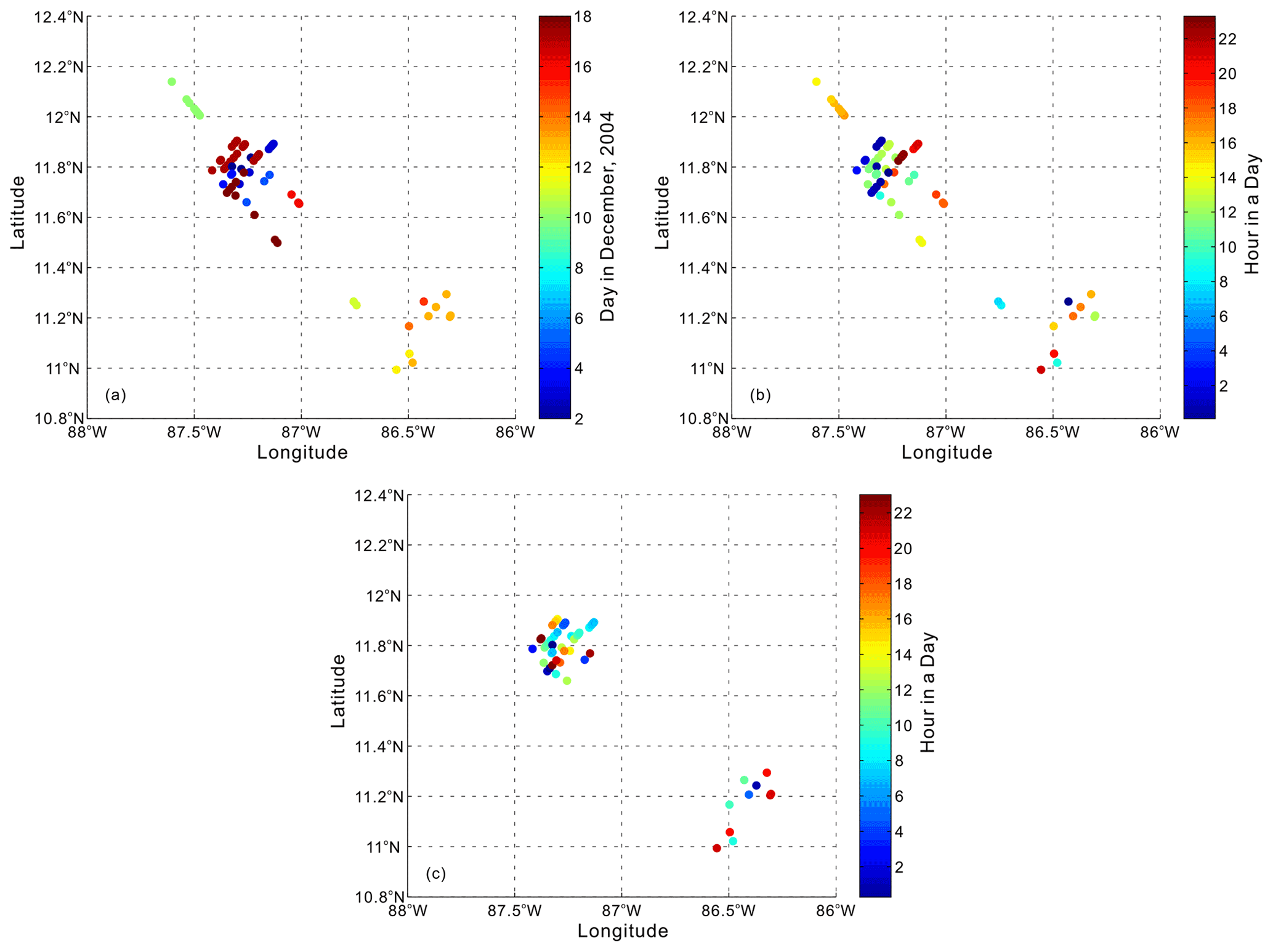
Figure 5 (a) The time at which the mode-2 ISWs observed in the study area appeared in days. (b) The time at which the mode-2 ISWs observed in the study area appeared in hours. (c) Tracing back the time (in hours) at which internal solitary waves appeared at the continental shelf break in the study area.

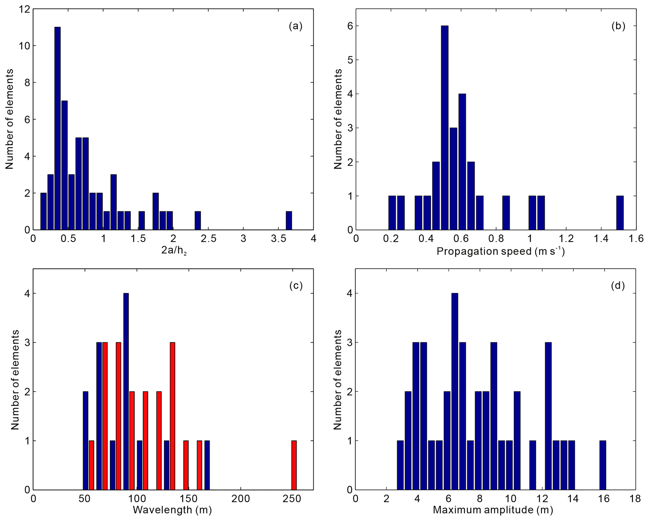
Figure 6 (a) Histogram of the dimensionless amplitude of the mode-2 ISW in the study area. (b) Histogram of the propagation speed of the mode-2 ISW in the study area. (c) Histogram of the wavelength of the mode-2 ISW in the study area. The dark blue and red bars denote the ISWs on the survey lines in the SW–NE and NE–SW directions, respectively. (d) Histogram of the maximum amplitude of the mode-2 ISW in the study area.

In addition to survey lines L74 and L84, the mode-2 ISWs also have sporadic distribution on other survey lines in the area (see the black filled circles in Fig. 1). We have identified 70 mode-2 ISWs in the study area. They appeared from 2 to 18 December 2004. On 17 and 18 December 2004, there were more mode-2 ISWs (Fig. 5a): 21 (10 for survey line L84, 6 for survey line L88, and 5 for survey line L76) and 9 (1 for survey line L72, 5 for survey line L76, and 3 for survey line L103), respectively. Observe the distribution of the appearance time of mode-2 ISWs observed in the study area in Fig. 5a (in days). We find that the mode-2 ISWs frequently appeared on the northwest side of the study area in December 2004, and appeared in early and late December. In addition, the spatial distribution range of the mode-2 ISWs is large, ranging from the continental slope to the continental shelf (see Figs. 1, 3, and 4). Figure 5b shows the time at which the mode-2 ISWs observed in the study area appeared in hours. Combined with Fig. 5a, we can find that from 2 to 8 December 2004, the ISWs appeared at around 12:00 and 00:00 GMT (Greenwich Mean Time)​​​​​​​ (or 24:00 GMT) in a day. From 10 to 13 December 2004, the ISWs appeared at around 12:00 and 24:00 GMT in a day, and relatively more appeared around 12:00 GMT. From 14 to 18 December 2004, the ISWs appeared at around 12:00 and 00:00 GMT (or 24:00 GMT) in a day, and relatively more appeared around 00:00 GMT (or 24:00 GMT). Survey lines L103, L105, and L107 are perpendicular to the propagation direction of the mode-2 ISWs in the study area (Fig. 1). Therefore, these three survey lines are not included in the subsequent statistical analysis of the mode-2 ISW characteristic parameters. We have counted the characteristic parameters of 53 mode-2 ISWs in the study area. In these 53 mode-2 ISWs, there are 51 small-amplitude ISWs ($\stackrel{\mathrm{̃}}{a}<\mathrm{2}$), and there are 40 ISWs with smaller amplitude ($\stackrel{\mathrm{̃}}{a}<\mathrm{1}$) among these 51 small-amplitude ISWs (Fig. 6a). The mode-2 ISWs in the study area are dominated by smaller amplitudes (Fig. 6a). The maximum amplitudes (in the vertical direction) of the mode-2 ISWs mainly change in the range of 3 to 13 m (Fig. 6d) and the equivalent wavelengths of most of the mode-2 ISWs are in the order of about 100 m (Fig. 6c, the equivalent wavelength in the figure has been corrected according to Eqs. 2 and 3). When calculating the propagation speed of the mode-2 ISW, due to the low signal-to-noise ratio of some survey lines, the calculation errors of some ISW propagation speeds are relatively large. Therefore, when analyzing the apparent propagation speed of the mode-2 ISW of the study area, we only used 26 ISWs with relatively small errors (the error is less than half of the calculated value). The apparent propagation speeds of the mode-2 ISWs in the study area are in the order of 0.5 m s⁻¹ (Fig. 6b), and most of the mode-2 ISWs propagate in the shoreward direction. We have traced back the time at which each ISW in the study area (mainly the ISWs located on the continental shelf) appeared at the continental shelf break using the ISW propagation speed of 0.5 m s⁻¹, as shown in Fig. 5c, in hours. Combined with Fig. 5a, we find that from 2 to 8 December 2004, the ISWs traced back to the continental shelf break appeared at around 12:00 and 00:00 GMT (or 24:00 GMT) in a day, and relatively more appeared around 12:00 GMT. From 10 to 13 December 2004, most of the ISWs traced back to the continental shelf break appeared at around 24:00 GMT (or 00:00 GMT) in a day. From 14 to 18 December 2004, the ISWs traced back to the continental shelf break appeared at around 12:00 and 24:00 GMT (or 00:00 GMT) in a day. The mode-2 ISWs observed in the study area may be generated by the interaction between the internal tide and the continental shelf break.

3.2 Propagation speed and wavelength characteristics of mode-2 ISWs in the study area

Inspired by the work of Maderich et al. (2015) and Chen et al. (2014), we calculated the relationships between the dimensionless propagation speed and the dimensionless amplitude $\stackrel{\mathrm{̃}}{a}$, the dimensionless wavelength λ₀ and the $\stackrel{\mathrm{̃}}{a}$, the propagation speed (U_c) and the maximum amplitude A, the wavelength (λ) and the A, the U_c and the pycnocline depth, and the U_c and the pycnocline thickness. Figure 7 shows the relationship between the dimensionless propagation speeds (we define the dimensionless propagation speed $\stackrel{\mathrm{̃}}{U}=U_{\mathrm{c}}/C$ for the convenience of using in the following text) and the dimensionless amplitudes $\stackrel{\mathrm{̃}}{a}$ of the observed 26 mode-2 ISWs (with relatively small errors) in the study area. When $\stackrel{\mathrm{̃}}{a}<\mathrm{1.18}$, it seems that the relationship between the $\stackrel{\mathrm{̃}}{U}$ values and the $\stackrel{\mathrm{̃}}{a}$ values of the observed mode-2 ISWs in the study area has the trends given by Kozlov and Makarov (1990) and Salloum et al. (2012), respectively; i.e., the $\stackrel{\mathrm{̃}}{U}$ of the mode-2 ISW increases with increasing $\stackrel{\mathrm{̃}}{a}$, but with different growth rates. The fitting effects of Kozlov and Makarov (1990), Salloum et al. (2012), and the segmentation fitting in Fig. 7 are shown in Table 3. The segmentation fitting computed by ourselves in Fig. 7 can be expressed by the equation as follows:

$$\begin{array}{}\text{(4)}& \stackrel{\mathrm{̃}}{U}={\displaystyle \frac{\mathrm{9.441}{\stackrel{\mathrm{̃}}{a}}^{\mathrm{4}}-\mathrm{27.19}{\stackrel{\mathrm{̃}}{a}}^{\mathrm{3}}+\mathrm{28.14}{\stackrel{\mathrm{̃}}{a}}^{\mathrm{2}}-\mathrm{10.93}\stackrel{\mathrm{̃}}{a}+\mathrm{1.016}}{\stackrel{\mathrm{̃}}{a}-\mathrm{0.6401}}}.\end{array}$$

When $\stackrel{\mathrm{̃}}{a}>\mathrm{1.18}$, the relationship between the $\stackrel{\mathrm{̃}}{U}$ values and the $\stackrel{\mathrm{̃}}{a}$ values of the observed mode-2 ISWs in the study area is closer to the result predicted by the deep-water weakly nonlinear theory (Benjamin, 1967). That is, the $\stackrel{\mathrm{̃}}{U}$ of the mode-2 ISW increases with increasing $\stackrel{\mathrm{̃}}{a}$ at a relatively small growth rate. The fitting effect of Benjamin (1967) in Fig. 7 is shown in Table 3. Figure 8 shows the relationship between the dimensionless wavelengths λ₀ and the dimensionless amplitudes $\stackrel{\mathrm{̃}}{a}$ of the 32 observed mode-2 ISWs (there are 13 ISWs on the survey lines in the SW–NE direction, and 19 ISWs on the survey lines in the NE–SW direction; see Fig. 6c) in the study area. In Fig. 8, the black and red crosses denote the ISWs on the survey lines in the SW–NE direction and in the NE–SW direction, respectively. The survey line in the SW–NE direction is consistent with the movement direction of the ISWs. Use Eq. (2) to correct the apparent wavelength to obtain the actual wavelength. The survey line in the NE–SW direction is opposite to the movement direction of the ISWs. Use Eq. (3) to correct the apparent wavelength to obtain the actual wavelength. Figure 8 shows the result after correcting the apparent wavelength of the ISW. When using Eqs. (2) and (3) to correct the apparent wavelength, the propagation speed of the ISW estimated in Fig. 7 needs to be used. The dimensionless wavelengths λ₀ of the ISWs with a large error in the estimation of the propagation speed are not shown in Fig. 8. Observing Fig. 8, it can be seen that when $\stackrel{\mathrm{̃}}{a}<\mathrm{1}$, the relationship between the λ₀ values and the $\stackrel{\mathrm{̃}}{a}$ values of the observed mode-2 ISWs in the study area is closer to the result predicted by the deep-water weakly nonlinear theory (Benjamin, 1967). However, the λ₀ values change from 2.5 to 7 for a fixed $\stackrel{\mathrm{̃}}{a}$ value. The fitting effect of Benjamin (1967) in Fig. 8 is shown in Table 4. When $\stackrel{\mathrm{̃}}{a}>\mathrm{1.87}$, the relationship between the λ₀ values and the $\stackrel{\mathrm{̃}}{a}$ values of the observed mode-2 ISWs in the study area is closer to the solution of Salloum et al. (2012). That is, the λ₀ of the mode-2 ISW increases with increasing $\stackrel{\mathrm{̃}}{a}$. The fitting effects of Salloum et al. (2012) and the segmentation fitting in Fig. 8 are shown in Table 4. The segmentation fitting computed by ourselves in Fig. 8 can be expressed by the equation as follows:

$$\begin{array}{}\text{(5)}& {\mathit{\lambda }}_{\mathrm{0}}=\mathrm{1.865}\stackrel{\mathrm{̃}}{a}+\mathrm{2.066}.\end{array}$$

When 1 < $\stackrel{\mathrm{̃}}{a}$ < 1.87, the λ₀ values of the observed mode-2 ISWs in the study area are higher than those predicted by the deep-water weakly nonlinear theory (Benjamin, 1967) and Salloum et al. (2012).

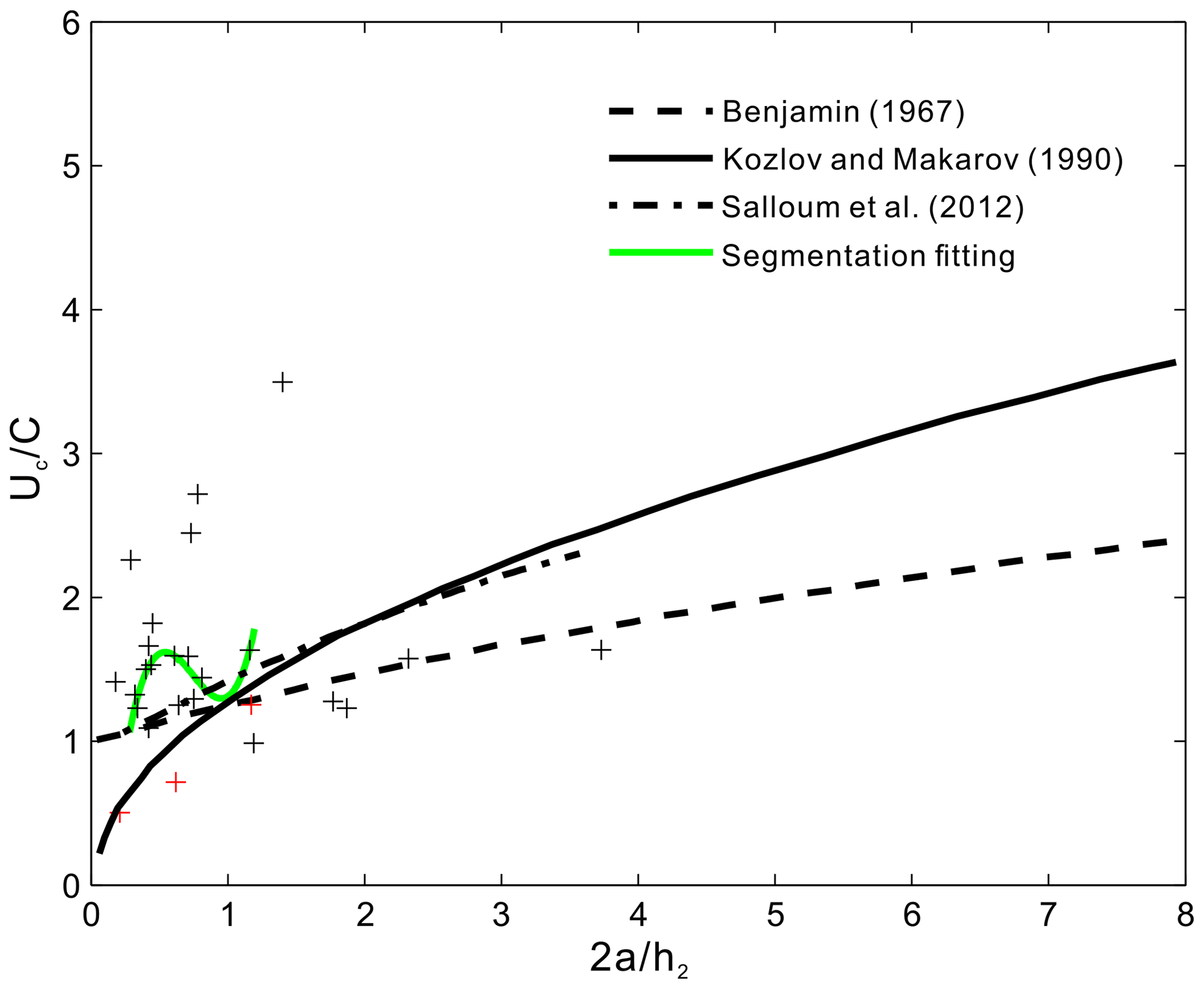
Figure 7 Relationship between the dimensionless propagation speeds and the dimensionless amplitudes of the mode-2 ISWs observed in the study area. The black and red crosses denote the seismic observation results of the mode-2 ISWs.

Table 3 Fitting effects of each curve in Fig. 7 on the observation points.

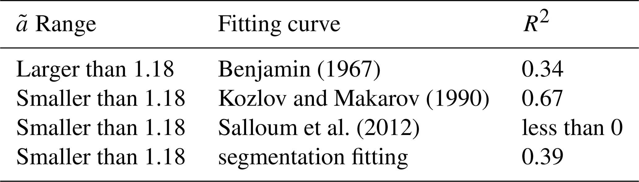
Note. For the fitting curve of Kozlov and Makarov (1990), we use the three red cross observation points to compute the R² value. For the fitting curves of Salloum et al. (2012) and segmentation fitting, we use the black cross observation points, whose $\stackrel{\mathrm{̃}}{U}$ are less than 2, to compute the R² values.

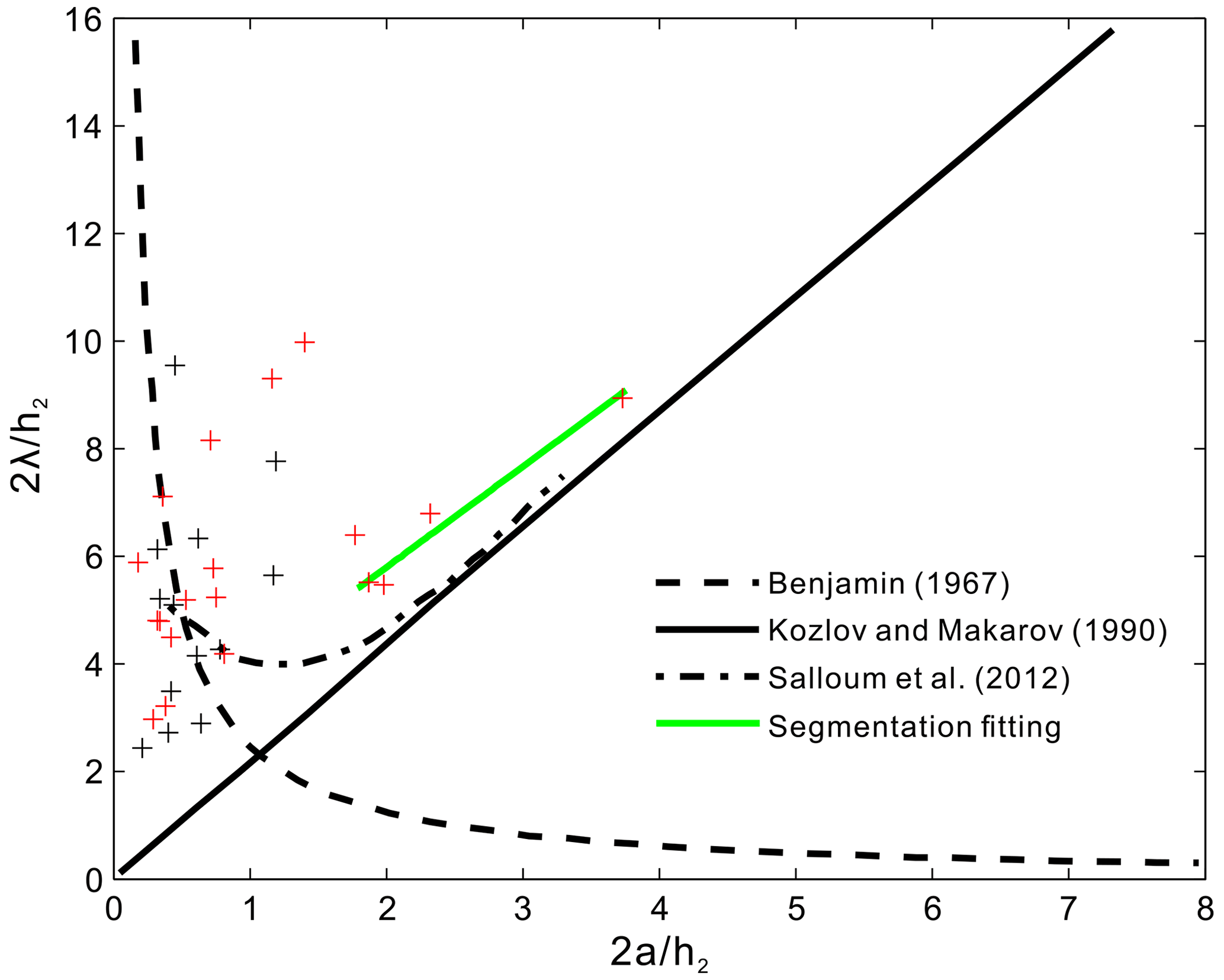
Figure 8 Relationship between the dimensionless wavelengths and the dimensionless amplitudes of the mode-2 ISWs observed in the study area. The black and red crosses denote the ISWs on the survey lines in the SW–NE and NE–SW directions, respectively.

Table 4 Fitting effects of each curve in Fig. 8 on the observation points.

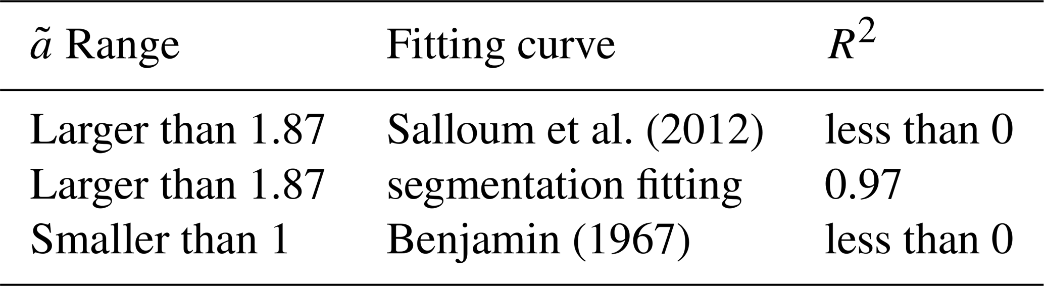
Figure 9 (a) Relationship between the propagation speeds and the maximum amplitudes of the mode-2 ISWs observed in the study area. (b) Relationship between the wavelengths and the maximum amplitudes of the mode-2 ISWs observed in the study area. The black and red triangles in panel (b) denote the ISWs on the survey lines in the SW–NE and NE–SW directions, respectively.

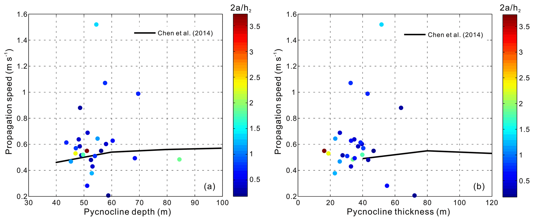
Figure 10 (a) Relationship between propagation speeds and pycnocline depths of the mode-2 ISWs observed in the study area. (b) Relationship between propagation speeds and pycnocline thicknesses of the mode-2 ISWs observed in the study area. The color-filled circles indicate the dimensionless amplitude.

The relationship between the propagation speeds U_c and the maximum amplitudes A of the mode-2 ISWs observed in the study area is shown in Fig. 9a. The relationship between the wavelengths λ and the maximum amplitudes A is shown in Fig. 9b. It can be seen that U_c and λ of the mode-2 ISW in the study area are less affected by A. There is no obvious linear correlation between U_c and A, or between λ and A (Fig. 9a and b). When the A values are between 6 and 11 m, the range of U_c is relatively large and there is a significant increase in U_c (Fig. 9a). When the A values are between 7 and 13 m, there is a significant increase in wavelength λ (Fig. 9b). The relationship between the propagation speeds U_c and the pycnocline depths h_c of the observed mode-2 ISWs in the study area is shown in Fig. 10a, and the relationship between the propagation speed U_c and the pycnocline thicknesses h₂ is shown in Fig. 10b. As for the observed mode-2 ISWs in the study area, their h_c values are mainly concentrated in the range of 40–70 m (Fig. 10a) and their h₂ values are mainly concentrated in the range of 10–60 m (Fig. 10b). As with the numerical simulation results of Chen et al. (2014), the U_c values of the observed mode-2 ISWs in the study area seem to have a trend to increase slowly with increasing h_c and h₂ values. The fitting effects of Chen et al. (2014) in Fig. 10 are shown in Table 5. The trends mentioned above are not completely monotonous in Fig. 10, as manifested in the large variation in U_c on the vertical axis. We postulate that this is due to the fact that other factors (such as seawater depth) in addition to pycnocline depth h_c and pycnocline thickness h₂ also affect the propagation speed U_c.

Table 5 Fitting effects of each curve in Fig. 10 on the observation points.

Note. For the fitting curve of Chen et al. (2014) in Fig. 10a, we use the observation points whose propagation speeds are less than 0.8 m s⁻¹ and larger than 0.21 m s⁻¹ to compute the R² value. For the fitting curve of Chen et al. (2014) in Fig. 10b, we use the observation points whose propagation speeds are less than 0.9 m s⁻¹ and pycnocline thicknesses are larger than 40 m to compute the R² value.

3.3 Vertical structure characteristics of the mode-2 ISW amplitude in the study area

The vertical distribution of ISW amplitude (the vertical displacement of isopycnal) is called its vertical structure. ISWs have different modes which correspond to different vertical structures (Fliegel and Hunkins, 1975). Previous scholars have used different theoretical models to study the vertical structure of ISW amplitude (Fliegel and Hunkins, 1975; Vlasenko et al., 2000; Small and Hornby, 2005). Among them, only Vlasenko et al. (2000) compared the results of numerical simulation with the results of local observations. They found that the depths corresponding to the ISW maximum amplitude (the maximum vertical displacement of isopycnals) given by the two are in good agreement. At present, there is less work comparing the theoretical vertical structure of mode-2 ISW amplitude with observed results. This work is conducive to improving our understanding of the vertical structure of the mode-2 ISW in the ocean (including the factors that affect the vertical structure). It can also test the validity and applicability of the theoretical vertical structure to a certain extent. The seismic oceanographic method has high spatial resolution, and its clear ISW imaging results are more conducive to the study of vertical structure. The vertical structure of ISW amplitude is controlled by a variety of environmental factors. Geng et al. (2019) used the seismic oceanography method to study the vertical structure of ISW amplitude near Dongsha Atoll in the South China Sea. They found that when the ISW interacts intensely with the seafloor, the observed vertical structure of ISW amplitude may be significantly different from the theoretical result. Gong et al. (2021) compared the vertical structure of ISW estimated by theoretical models with the vertical structure of ISW observed by the seismic oceanography method. They analyzed in detail the factors affecting the vertical structure of ISW amplitude near Dongsha Atoll in the South China Sea and found that the vertical structure of ISW is mainly controlled by nonlinearity. It usually appears that the quadratic nonlinear coefficients of ISWs that conform to the linear vertical structure function are small, while the quadratic nonlinear coefficients of ISWs conforming to the first-order nonlinear vertical structure function are larger. In addition, topography, ISW amplitude, seawater depth, and background flow may all affect the vertical structure of ISW amplitude. It appears that larger seawater depth may weaken the influence of the nonlinearity of the ISW on the vertical structure, making the vertical structure of ISW more in line with linear theory. Larger amplitude will make ISW more susceptible to the influence of topography, which will change the vertical structure. Vlasenko et al. (2000) observed that the vertical structure of ISW has local extrema, which they thought to be caused by smaller-scale internal waves. In addition, the background flow shear also has an important effect on the vertical structure (Stastna and Lamb, 2002; Liao et al., 2014). Xu et al. (2020) found that the background flow at the center of the eddy can weaken the amplitude of ISW.

Figure 11 Panels (a)–(j) demonstrate the vertical structure characteristics of the amplitude of the 10 mode-2 ISWs ISW1–ISW10 on survey line L84 as well as the vertical mode function fitting results. The black circles denote the observed ISWs' amplitudes at different depths. The blue curves are the linear vertical mode function (nonlinear correction is not considered) and the red curves are the first-order nonlinear vertical mode function (nonlinear correction is considered).

Observing the vertical structure of the mode-2 ISW amplitude in the study area, we find that it follows the following characteristics as a whole: the amplitude of ISWs in the upper half of the pycnocline decreases with increasing seawater depth; the amplitude of ISWs in the lower half of the pycnocline first increases, and then decreases with increasing seawater depth (see Figs. 11 and 12 in this paper, Fig. 5 of Fan et al., 2021a, and Fig. 6 of Fan et al., 2021b). Due to the influence of the pycnocline center deviation on development of the vertical structure of ISW amplitude, the vertical structure of the mode-2 ISW amplitude in the study area generally only exhibits a part of the characteristics given by the vertical mode function. As for the vertical mode function, the amplitude of the ISW in the upper and lower half of the pycnocline firstly increases and then decreases with the increasing seawater depth, as shown by the blue and red curves in Figs. 11 and 12. Since the pycnocline centers of most of the mode-2 ISWs observed in the study area deviate upwards, the ISW structure at the top is not as well developed as the ISW structure at the bottom. Therefore, the amplitude of the ISW in the upper half of the pycnocline usually decreases with increasing seawater depth. Figure 11 shows the vertical structures of the amplitude of the 10 mode-2 ISWs ISW1–ISW10 in survey line L84. The pycnocline centers corresponding to ISW1–ISW7 all deviate upwards (see the degree to which the mid-depth of the pycnocline deviates from $\mathrm{1}/\mathrm{2}$ seafloor depth in Table 1; the positive sign indicates that the pycnocline deviates upward and the negative sign indicates that the pycnocline deviates downward). Among them, ISW1–ISW4 (Fig. 11a–d) and ISW7 (Fig. 11g) only have one reflection event in the upper half of the pycnocline. From ISW6 (Fig. 11f), we can see that the amplitude of ISWs in the upper half of the pycnocline decreases with increasing seawater depth. From ISW2 (Fig. 11b), ISW4 (Fig. 11d), ISW5 (Fig. 11e), and ISW7 (Fig. 11g), it can be seen that the amplitude of ISW in the lower half of the pycnocline firstly increases and then decreases with the increasing seawater depth. The pycnocline centers corresponding to ISW8–ISW10 all deviate slightly downwards (see the degree to which the mid-depth of the pycnocline deviates from $\mathrm{1}/\mathrm{2}$ seafloor depth in Table 1; the positive sign indicates that the pycnocline deviates upward and the negative sign indicates that the pycnocline deviates downward). From ISW8 (Fig. 11h) and ISW10 (Fig. 11j), it can be seen that the amplitude of the ISW in the upper half of the pycnocline decreases with increasing seawater depth. Figure 12 shows the vertical structures of the amplitude of the four mode-2 ISWs (ISW11, ISW12, ISW16, and ISW17) in survey line L74. The pycnocline centers corresponding to ISW11, ISW12, ISW16, and ISW17 deviate significantly downwards (see the degree to which the mid-depth of the pycnocline deviates from 1/2 seafloor depth in Table 2; the positive sign indicates that the pycnocline deviates upward and the negative sign indicates that the pycnocline deviates downward). This renders the ISW structure at the top more developed. From ISW11, ISW12, and ISW17 (Fig. 12a, b, d), it can be seen that the amplitude of the ISW in the upper half of the pycnocline first increases and then decreases with increasing seawater depth.

Figure 12 Panels (a)–(d) demonstrate the vertical structure characteristics of the amplitude of the four mode-2 ISWs (ISW11, ISW12, ISW16, and ISW17) on survey line L74 as well as the vertical mode function fitting results. The black circles denote the observed ISWs' amplitudes at different depths. The blue curves are the linear vertical mode function (nonlinear correction is not considered) and the red curves are the first-order nonlinear vertical mode function (nonlinear correction is considered).

To study the vertical structure of the mode-2 ISW amplitude in more detail for the study area, we compare the observation result with the linear vertical mode function (nonlinear correction is not considered, the blue curves in Figs. 11 and 12) and the first-order nonlinear vertical mode function (considering nonlinear correction, the red curves in Figs. 11 and 12). The linear vertical mode function can be obtained by solving the eigenvalue equation that satisfies the Taylor–Goldstein problem (Holloway et al., 1999):

$$\begin{array}{}\text{(6)}& \begin{array}{rl}& {\displaystyle \frac{{\mathrm{d}}^{\mathrm{2}}\mathit{\phi }\left(z\right)}{\mathrm{d}{z}^{\mathrm{2}}}}+{\displaystyle \frac{N^{\mathrm{2}}\left(z\right)}{C^{\mathrm{2}}}}\mathit{\phi }\left(z\right)=\mathrm{0}\\ & \mathit{\phi }\left(\mathrm{0}\right)=\mathit{\phi }(-H)=\mathrm{0},\end{array}\end{array}$$

where φ(z) represents the linear vertical mode function, C is the linear phase speed, and N(z) is the Brunt–Väisälä frequency. We use the temperature and salinity data coming from the Copernicus Marine Environment Monitoring Service (CMEMS) to compute the Brunt–Väisälä frequency. The first-order nonlinear vertical mode function is obtained by adding a nonlinear correction term to the linear vertical mode function (Lamb and Yan, 1996). It can be expressed by the following equation:

$$\begin{array}{}\text{(7)}& {\mathit{\phi }}_m\left(z\right)=\mathit{\phi }\left(z\right)+{\mathit{\eta }}_{\mathrm{0}}T\left(z\right),\end{array}$$

where η₀ is the ISW maximum amplitude in the vertical direction and T(z) is the first-order nonlinear correction term. T(z) satisfies equations as follows (Grimshaw et al., 2002, 2004):

$$\begin{array}{}\text{(8)}& {\displaystyle }\begin{array}{rl}{\displaystyle \frac{{\mathrm{d}}^{\mathrm{2}}T\left(z\right)}{\mathrm{d}{z}^{\mathrm{2}}}}+{\displaystyle \frac{N(z{)}^{\mathrm{2}}}{C^{\mathrm{2}}}}T\left(z\right)& =-{\displaystyle \frac{\mathit{\alpha }}{C}}{\displaystyle \frac{{\mathrm{d}}^{\mathrm{2}}\mathit{\phi }\left(z\right)}{\mathrm{d}{z}^{\mathrm{2}}}}\\ & +{\displaystyle \frac{\mathrm{3}}{\mathrm{2}}}{\displaystyle \frac{\mathrm{d}}{\mathrm{d}z}}\left[{\left({\displaystyle \frac{\mathrm{d}\mathit{\phi }\left(z\right)}{\mathrm{d}z}}\right)}^{\mathrm{2}}\right]\end{array}\text{(9)}& {\displaystyle }\begin{array}{rl}& T\left(\mathrm{0}\right)=T(-H)=\mathrm{0}\\ & \mathit{\alpha }={\displaystyle \frac{\mathrm{3}C}{\mathrm{2}}}{\displaystyle \frac{{\int }_{-H}^{\mathrm{0}}{\left(\frac{\mathrm{d}\mathit{\phi }\left(z\right)}{\mathrm{d}z}\right)}^{\mathrm{3}}\mathrm{d}z}{{\int }_{-H}^{\mathrm{0}}{\left(\frac{\mathrm{d}\mathit{\phi }\left(z\right)}{\mathrm{d}z}\right)}^{\mathrm{2}}\mathrm{d}z}},\end{array}\end{array}$$

where α is the quadratic nonlinear coefficient. Equation (8) has a unique solution by adding the restriction condition of $T\left(z_{max}\right)=\mathrm{0}$ (Grimshaw et al., 2002), where z_max represents the depth of the maximum amplitude of ISW. The detailed calculation process is described in Gong et al. (2021). The fitting effects of the linear vertical mode function and the first-order nonlinear vertical mode function in Fig. 11 are shown in Table 6. We comprehensively evaluate the goodness of fit by the computed R², the depths corresponding to the maximum amplitude between the observation results and the fitting results, and the overall trends between the observation results and the fitting results. Observing Fig. 11 and Table 6, we find that the overall nonlinearity of the ISWs ISW5 (Fig. 11e) and ISW8 (Fig. 11h) on survey line L84 is relatively strong, and the first-order nonlinear vertical mode function considering nonlinear correction can be used to better fit the vertical structure of the amplitude (the red curves in Fig. 11e, h). The nonlinearity is relatively strong at the bottom of ISW2 (the seawater depth range is 60–80 m in Fig. 11b), the top of ISW7 (the seawater depth range is 40–60 m in Fig. 11g), and the top of ISW10 (the seawater depth is about 40 m in Fig. 11j), and the first-order nonlinear vertical mode function considering nonlinear correction can be used to better fit the vertical structure of the amplitude (the red curves in Fig. 11b, g, j). The overall nonlinearity of ISW1 (Fig. 11a), ISW3 (Fig. 11c), ISW6 (Fig. 11f), and ISW9 (Fig. 11i) is relatively weak, and the linear vertical mode function can be used to better fit the vertical structure of the amplitude (the blue curves in Fig. 11a, c, f, i). The nonlinearity is relatively weak at the top of ISW2 (the seawater depth range is 40–60 m in Fig. 11b), the bottom of ISW7 (the seawater depth range is 60–90 m in Fig. 11g), and the bottom of ISW10 (the seawater depth is below 40 m in Fig. 11j). The linear vertical mode function can be used to better fit the vertical structure of the amplitude (the blue curves in Fig. 11b, g, j). The above analysis reflects that the vertical structure of the mode-2 ISW amplitude in the study area is affected by the degree of nonlinearity of the ISW. The fitting effects of the linear vertical mode function and the first-order nonlinear vertical mode function in Fig. 12 are shown in Table 7. We comprehensively evaluate the goodness of fit by the computed R², the depths corresponding to the maximum amplitude between the observation results and the fitting results, and the overall trends between the observation results and the fitting results. Observing Fig. 12 and Table 7, we find that neither the linear vertical mode function (without considering nonlinear correction) nor the first-order nonlinear vertical mode function (with consideration of nonlinear correction) can be used to fit the vertical structure of the amplitude of the ISWs ISW11, ISW12, ISW16, and ISW17 on L74 well (especially the position of the upper half of the pycnocline). The ISWs ISW11, ISW12, ISW16, and ISW17 on survey line L74 have a large downward deviation of the pycnocline center (see the degree to which the mid-depth of the pycnocline deviates from $\mathrm{1}/\mathrm{2}$ seafloor depth in Table 2; the positive sign indicates that the pycnocline deviates upward and the negative sign indicates that the pycnocline deviates downward). We have observed the fitting result of the vertical amplitude of the ISW with the large downward pycnocline deviation on other lines of the study area (not shown in this article) and found that the fitting result of the vertical amplitude is usually poorer than that of the ISW corresponding to the upward deviation of the pycnocline (especially the position of the upper half of the pycnocline). We believe that when the pycnocline center has a large downward deviation, the vertical mode function (including the linear vertical mode function without considering nonlinear correction, and the first-order nonlinear vertical mode function considering nonlinear correction) cannot be used to well fit the vertical structure of the mode-2 ISW amplitude in the study area. The above analysis once again reflects that the pycnocline deviation (especially the downward deviation of the pycnocline) affects the vertical structure of the mode-2 ISW amplitude in the study area. In addition, we could not find a good way to fit the vertical amplitude structure in Fig. 12 based on the basic KdV theory. Another theory may be needed to fit this kind of vertical amplitude structure. We hope this can be solved in future studies.

Table 6 Fitting effects of each curve in Fig. 11 on the observation points.

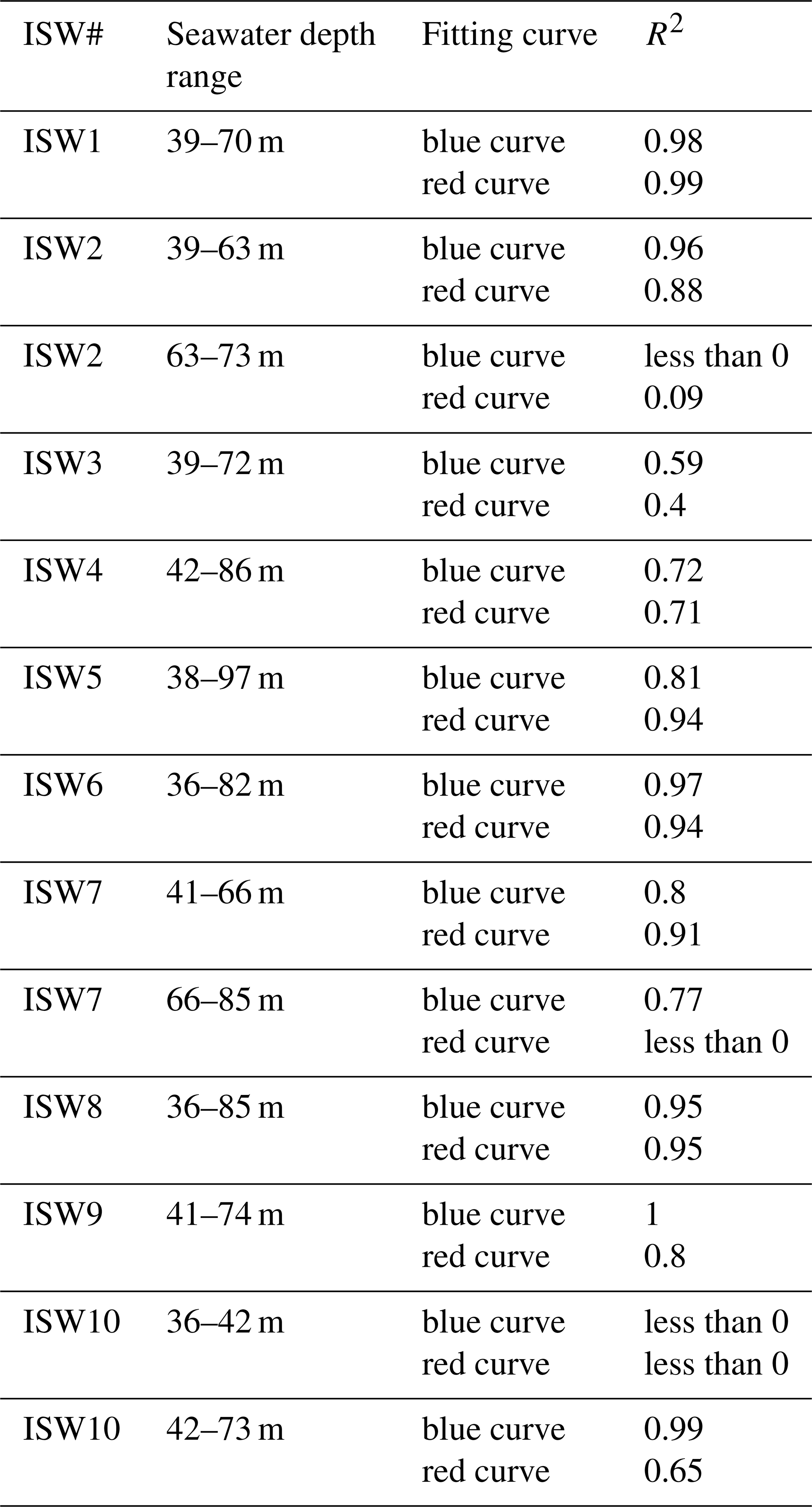
Table 7 Fitting effects of each curve in Fig. 12 on the observation points.

4 Discussion

Regarding the relationship between the dimensionless propagation speed $\stackrel{\mathrm{̃}}{U}$ and dimensionless amplitude $\stackrel{\mathrm{̃}}{a}$ of the mode-2 ISW in the study area, as well as the relationship between the dimensionless wavelength λ₀ and dimensionless amplitude $\stackrel{\mathrm{̃}}{a}$, neither is strictly monotonous in the case of smaller amplitude ($\stackrel{\mathrm{̃}}{a}<\mathrm{1}$) and both show the characteristics of multi-parameter controlling (Figs. 7 and 8). For this reason, we analyzed the influence of seawater depth (seafloor depth) on $\stackrel{\mathrm{̃}}{U}$ and λ₀ of the mode-2 ISWs in the study area. The results are shown in Fig. 13a and b, respectively. Observing Fig. 13a, we find that in shallow seawater (seafloor depth less than 120 m), the $\stackrel{\mathrm{̃}}{U}$ variation range is small and there are both large-amplitude mode-2 ISWs ($\stackrel{\mathrm{̃}}{a}>\mathrm{2}$) and small-amplitude mode-2 ISWs ($\stackrel{\mathrm{̃}}{a}<\mathrm{2}$). In deep seawater (or at the shelf break; seafloor depth is greater than 120 m), the smaller-amplitude mode-2 ISWs ($\stackrel{\mathrm{̃}}{a}$ < 1; dark blue filled circles in Fig. 13a) have a large $\stackrel{\mathrm{̃}}{U}$ variation range. The maximum $\stackrel{\mathrm{̃}}{U}$ can reach 2.45, and the minimum can reach 0.5. In particular, the smaller $\stackrel{\mathrm{̃}}{U}$ values are mainly concentrated in the deep seawater, so that in Fig. 7, when $\stackrel{\mathrm{̃}}{a}$ < 1.18, the relationship between $\stackrel{\mathrm{̃}}{U}$ and $\stackrel{\mathrm{̃}}{a}$ of the mode-2 ISW seems to have the trend given by Kozlov and Makarov (1990). The sharp decrease in the $\stackrel{\mathrm{̃}}{U}$ values of the mode-2 ISWs with smaller amplitudes in deep seawater may be caused by collision of the ISWs with the seafloor topography (including the step) at the shelf break. In addition, from Fig. 10a and b, it can be seen that on the whole, the pycnocline depths and the pycnocline thicknesses of the larger-amplitude mode-2 ISWs ($\stackrel{\mathrm{̃}}{a}$ > 1) are smaller than the pycnocline depths and the pycnocline thicknesses of the smaller-amplitude mode-2 ISWs ($\stackrel{\mathrm{̃}}{a}$ < 1). Therefore, the propagation speeds of the larger-amplitude mode-2 ISWs ($\stackrel{\mathrm{̃}}{a}$ > 1) are generally smaller than the propagation speeds of the smaller-amplitude mode-2 ISWs ($\stackrel{\mathrm{̃}}{a}$ < 1). In Fig. 7, when $\stackrel{\mathrm{̃}}{a}$ > 1.18, this makes the relationship between $\stackrel{\mathrm{̃}}{U}$ and $\stackrel{\mathrm{̃}}{a}$ of the mode-2 ISWs closer to the result predicted by the deep-water weakly nonlinear theory (Benjamin, 1967). The above-analyzed influences of seawater depth (seafloor topography), pycnocline depth, and pycnocline thickness on the mode-2 ISW propagation speed in the study area have caused the diversity of the relationship between $\stackrel{\mathrm{̃}}{U}$ and $\stackrel{\mathrm{̃}}{a}$: when $\stackrel{\mathrm{̃}}{a}$ < 1.18, the relationship between the $\stackrel{\mathrm{̃}}{U}$ values and the $\stackrel{\mathrm{̃}}{a}$ values of the observed mode-2 ISWs in the study area seems to have the trends given by Kozlov and Makarov (1990) and Salloum et al. (2012); when $\stackrel{\mathrm{̃}}{a}$ > 1.18, the relationship between the $\stackrel{\mathrm{̃}}{U}$ values and the $\stackrel{\mathrm{̃}}{a}$ values of the observed mode-2 ISWs in the study area is closer to the result predicted by the deep-water weakly nonlinear theory (Benjamin, 1967).

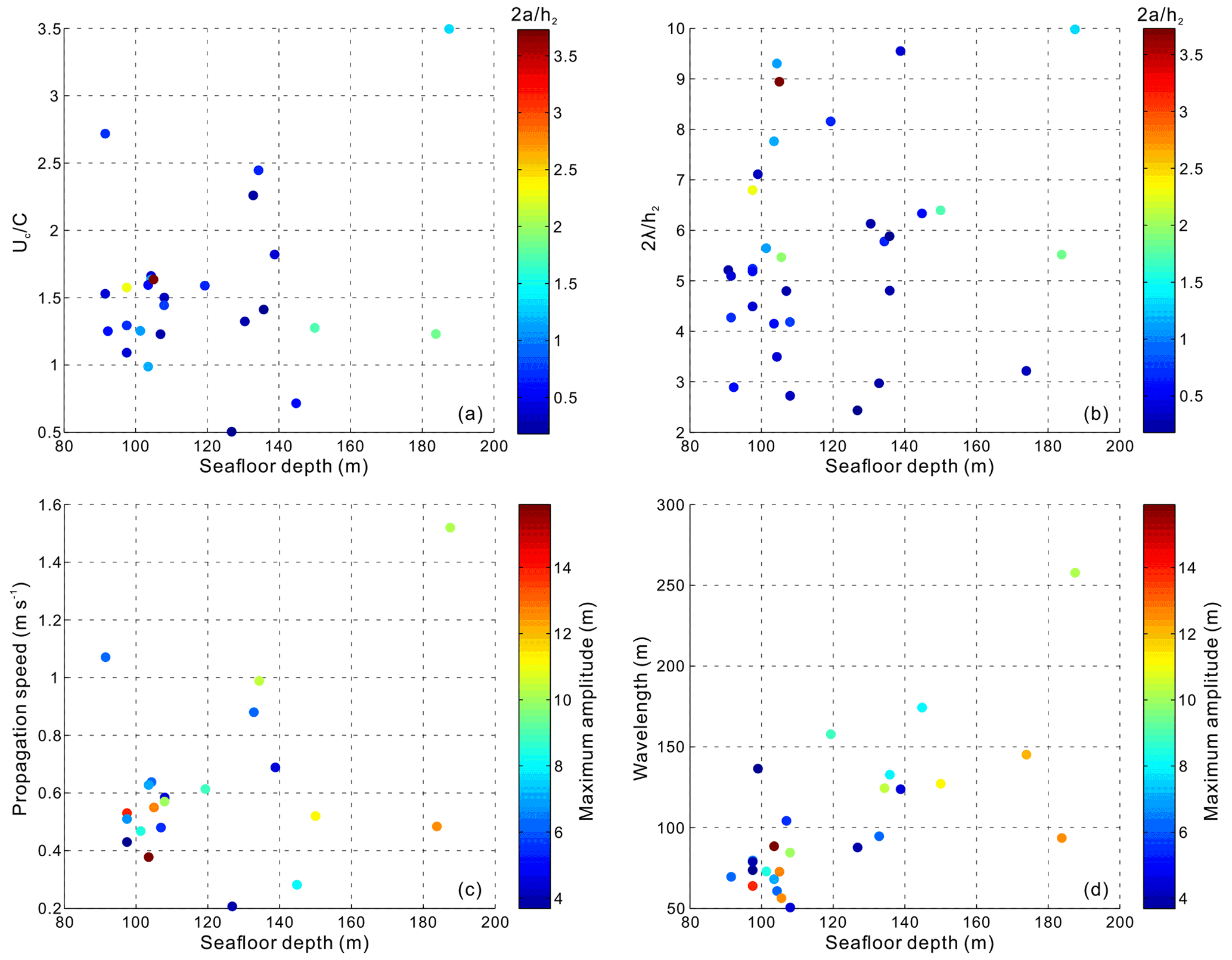
Figure 13 (a) Relationship between dimensionless propagation speeds and seawater depths of the mode-2 ISWs observed in the study area. The color of the filled circle indicates the dimensionless amplitude. (b) Relationship between dimensionless wavelengths and seawater depths of the mode-2 ISWs observed in the study area. The color of the filled circle indicates the dimensionless amplitude. (c) Relationship between propagation speeds and seawater depths of the mode-2 ISWs observed in the study area. The color of the filled circle indicates the maximum amplitude. (d) Relationship between wavelengths and seawater depths of the mode-2 ISWs observed in the study area. The color of the filled circle indicates the maximum amplitude.

Observing Fig. 13b, we find that the mode-2 ISWs with smaller amplitudes ($\stackrel{\mathrm{̃}}{a}$ < 1; dark blue filled circles in Fig. 13b) have a relatively large variation range of the dimensionless wavelength λ₀ in deep seawater (seafloor depth greater than 120 m). The largest λ₀ can reach up to 9.55 (corresponding to ISW2 on survey line L84, whose pycnocline deviation is large and waveform is asymmetric), and the smallest λ₀ can reach 2.44, so that the λ₀ of the vertical axis in Fig. 8 can be reduced to 2.44 when $\stackrel{\mathrm{̃}}{a}$ < 1. The sharp decrease in the λ₀ values of the mode-2 ISWs with smaller amplitudes ($\stackrel{\mathrm{̃}}{a}$ < 1) in deep seawater may be caused by collision of the ISWs with the seafloor topography at the shelf break. The sharp increase in λ₀ values of the mode-2 ISWs with smaller amplitudes in deep seawater may be related to the waveform asymmetry caused by the pycnocline deviation.

Figure 13c and d show the relationship between propagation speed U_c and seawater depth, and between wavelength λ and seawater depth of the mode-2 ISWs in the study area, respectively. The color of the filled circles in the figures represents the maximum amplitude. Observing Fig. 13c, we find that the seawater depth in the study area has a great influence on the U_c of the mode-2 ISWs. In the shallow seawater area (seawater depth less than 120 m), the U_c range is small. In the deep seawater area (seawater depth greater than 120 m),U_c has a large range. The maximum U_c is 1.52 m s⁻¹ and the minimum U_c is 0.21 m s⁻¹. In Fig. 9a, when the maximum amplitude is between 6 and 11 m, U_c has a large range and there is a significant increase in U_c. The above phenomenon is controlled by seawater depth, i.e., in the deep seawater area (seawater depth greater than 120 m), for the ISWs with a maximum amplitude of 6–11 m, U_c varies widely and the maximum U_c of 1.52 m s⁻¹ appears (Fig. 13c). Observing Fig. 13d, we find that the seawater depth in the study area has a great influence on the wavelength λ of the mode-2 ISW. On the whole, the λ of the ISW increases with increasing seawater depth. For the ISWs with a maximum amplitude of 7–13 m, considerable parts of the waves are distributed in the deep seawater area (seawater depth is greater than 120 m), making their λ values increase significantly. As a result, when the maximum amplitude is between 7 and 13 m in Fig. 9b, there is a significant increase in the wavelength λ.

McSweeney et al. (2020a, b) conducted observational studies on the cross-shore and alongshore evolution characteristics of internal bores near Point Sal, California. They used the quadratic nonlinear coefficient α calculated by the KdV theory to characterize the stratification, and found that when the α calculated from the background density is greater than 0, the waveform of the internal bore becomes steep as the internal bore passes the site. When the α calculated from the background density is less than 0, the waveform of the internal bore becomes rarefied as the internal bore passes the site. Background stratification affects the evolution of internal bores and the passage of an internal bore will also change the stratification, which, in turn, affects the evolution of a subsequent internal bore. They found that the change in α after the internal bore had passed is positively correlated with the background α. By analogy with the work of McSweeney et al. (2020a, b), we calculated the background quadratic nonlinear coefficient α (corresponding to the stratification before the arrival of the ISW) and the linear phase speed C at the position of the ISWs in the study area by solving Eqs. (6) and (9). Because the theoretical vertical structures calculated based on KdV theory cannot well describe the ISWs appearing on the survey line L74 (Fig. 12), we have only calculated α and C at each ISW position on survey line L84. The calculation results are shown in columns 12 and 13 of Table 1, respectively. Observing the calculated α values in Table 1, we find that the α values of ISW1-ISW4 are all less than 0. And the α values of ISW5-ISW10 are all greater than 0. It corresponds well to the waveform characteristics of the ISWs in Fig. 3. That is, for ISW1–ISW4, whose α values are less than 0, their waveforms are relatively rarefied. For ISW5–ISW10, whose α values are greater than 0, their waveforms are relatively steep. This indicates that background stratification has an influence on the shape of the mode-2 ISWs in the study area. Observing the calculated C values in Table 1, we find that from ISW1 to ISW4, the calculated C values gradually decrease with decreasing seafloor depths. This is consistent with the observed trend that the propagation speeds U_c of the ISWs (column 11 of Table 1) also gradually decrease with decreasing seafloor depths. ISW5 is shallower than ISW4, but the calculated C and the observed U_c of ISW5 are both greater than those of ISW4. From ISW5 to ISW10, as the seafloor depth gradually decreases, the calculated C values and the observed ISW U_c values again show an overall decreasing trend. We think the above phenomenon is caused by background stratification, as ISW1–ISW4 have a similar background stratification and ISW5–ISW10 have another similar background stratification. This makes the calculated C values and observed U_c values of SW1–ISW4 decrease with decreasing seafloor depth. The calculated C and observed U_c of ISW5 are greater than those of ISW4. On the whole, the calculated C values and the observed U_c values of ISW5–ISW10 decrease with decreasing seafloor depth. The above discussion indicates that background stratification has an influence on the propagation speed of mode-2 ISWs in the study area.

5 Conclusions

We carried out a regional study of mode-2 ISWs at the Pacific coast of Central America using the seismic reflection method. Via analysis of the typical seismic sections L84 and L74, we find that when the degree of downward pycnocline deviation is large, the influence of pycnocline deviation on the stability of the mode-2 ISW is more complicated than when the pycnocline deviates upwards – there are mode-2 ISWs with a large degree of downward pycnocline deviation, but with a relatively symmetrical waveform.

The observed relationship between dimensionless propagation speed $\stackrel{\mathrm{̃}}{U}$ and dimensionless amplitude $\stackrel{\mathrm{̃}}{a}$ of the mode-2 ISWs in the study area was analyzed. When $\stackrel{\mathrm{̃}}{a}$ < 1.18, $\stackrel{\mathrm{̃}}{U}$ seems to increase with increasing $\stackrel{\mathrm{̃}}{a}$, divided into two parts with different growth rates. When $\stackrel{\mathrm{̃}}{a}$ > 1.18, $\stackrel{\mathrm{̃}}{U}$ increases with increasing $\stackrel{\mathrm{̃}}{a}$ at a relatively small growth rate. The observed relationship between dimensionless wavelength λ₀ and dimensionless amplitude $\stackrel{\mathrm{̃}}{a}$ of the mode-2 ISWs in the study area was also analyzed. When $\stackrel{\mathrm{̃}}{a}$ < 1, λ₀ seems to change from 2.5 to 7 for a fixed $\stackrel{\mathrm{̃}}{a}$ value. When $\stackrel{\mathrm{̃}}{a}$ > 1.87, λ₀ increases with increasing $\stackrel{\mathrm{̃}}{a}$. As for the relationships between $\stackrel{\mathrm{̃}}{U}$ and $\stackrel{\mathrm{̃}}{a}$, and λ₀ and $\stackrel{\mathrm{̃}}{a}$ of the mode-2 ISWs in the study area, both show the characteristics of multi-parameter controlling. Seawater depth (seafloor topography), pycnocline depth, and pycnocline thickness all have an influence on the mode-2 ISW propagation speed in the study area. This causes the diversity of the relationship between $\stackrel{\mathrm{̃}}{U}$ and $\stackrel{\mathrm{̃}}{a}$.

The vertical structure of the mode-2 ISW amplitude in the study area is affected by the degree of nonlinearity of the ISW. The first-order nonlinear vertical mode function considering nonlinear correction can be used to better fit the vertical amplitude structure of the mode-2 ISWs with strong nonlinearity. The first-order nonlinear vertical mode function can also be used to better fit the vertical amplitude structure of the ISW position with strong nonlinearity in the vertical direction. The pycnocline deviation (especially the downward deviation of the pycnocline) affects the vertical structure of the mode-2 ISW amplitude in the study area. When the pycnocline center has a large downward deviation, the vertical mode function cannot be used to well fit the vertical structure of the mode-2 ISW amplitude in the study area.