the Creative Commons Attribution 4.0 License.
the Creative Commons Attribution 4.0 License.
 | 08 Feb 2021
Behavior of the iterative ensemble-based variational method in nonlinear problems
The behavior of the iterative ensemble-based data assimilation algorithm is discussed. The ensemble-based method for variational data assimilation problems, referred to as the 4D ensemble variational method (4DEnVar), is a useful tool for data assimilation problems. Although the 4DEnVar is derived based on a linear approximation, highly uncertain problems, in which system nonlinearity is significant, are solved by applying this method iteratively. However, the ensemble-based methods basically seek the solution within a lower-dimensional subspace spanned by the ensemble members. It is not necessarily trivial how high-dimensional problems can be solved with the ensemble-based algorithm which employs the lower-dimensional approximation based on the ensemble. In the present study, an ensemble-based iterative algorithm is reformulated to allow us to analyze its behavior in high-dimensional nonlinear problems. The conditions for monotonic convergence to a local maximum of the objective function are discussed in a high-dimensional context. It is shown that the ensemble-based algorithm can solve high-dimensional problems by distributing the ensemble in different subspace at each iteration. The findings as the results of the present study were also experimentally supported.
- Article
(2163 KB) - Full-text XML
- BibTeX
- EndNote


The 4D ensemble variational method (4DEnVar; Lorenc, 2003; Liu et al., 2008) is a useful tool for practical data assimilation. The 4DEnVar obtains the derivative of the objective function from the approximate Jacobian of a dynamical system model, which is estimated by using the ensemble of simulation results. In contrast with the adjoint method, the 4DEnVar does not require an adjoint code which is usually time-consuming to develop. This ensemble method thus allows us to treat the simulation code as a black box, and it can easily be implemented.
The 4DEnVar algorithm is derived based on a low-dimensional linear approximation of the high-dimensional nonlinear system model. If the uncertainties in state variables are small, then the solution could be found within the range where a linear approximation is valid. However, geophysical systems are often highly uncertain. If the scale of uncertainty is much larger than the range of linearity, a linear approximation would not be justified. In atmospheric applications, uncertainty can usually be reduced by taking sufficient spin-up time. On the other hand, in some geophysical applications, it is difficult to obtain a sufficiently long sequence of observations to allow spin-up. For example, in data assimilation for the interior of the Earth, such as lithospheric plates (e.g., Kano et al., 2015) and the outer core (e.g., Sanchez et al., 2019; Minami et al., 2020), the timescale of the system dynamics is so long that a sufficient length of an observation sequence is not feasible. It is also difficult to use a long sequence of observations in the Earth's magnetosphere where the amount of observations is limited (e.g., Nakano et al., 2008; Godinez et al., 2016). It is therefore an important issue to consider large uncertainties which could deteriorate the validity of the linear approximation.
Several studies have suggested that estimations in nonlinear problems can be improved by iterative algorithms in which the ensemble is repeatedly updated in each iteration (e.g., Gu and Oliver, 2007; Kalnay and Yang, 2010; Chen and Oliver, 2012; Bocquet and Sakov, 2013, 2014; Raanes et al., 2019). These iterative algorithms can be regarded as a variant of the 4DEnVar method, based on an approximation of the Gauss–Newton method or the Levenberg–Marquardt method. The Gauss–Newton and the Levenberg–Marquardt methods are variants of the Newton–Raphson method for solving nonlinear least squares problems by using the Jacobian of a nonlinear function. Thus, when the Gauss–Newton or the Levenberg–Marquardt framework is strictly applied to data assimilation problems, the tangent linear of the system model is required. Indeed, if the tangent linear of the system model is obtained, 4D variational data assimilation problems can be solved with the incremental formulation (Courtier et al., 1994), which can be regarded as an instance of the Gauss–Newton framework (Lawless et al., 2005). The ensemble-based methods avoid computing the Jacobian of a nonlinear system model by a linear approximation using the ensemble. This ensemble-based approximation is justified if linearity can be assumed over the range where the ensemble members are distributed. However, the ensemble-based methods basically seek the solution within a lower-dimensional subspace spanned by the ensemble members. In many applications in atmospheric sciences, it has been demonstrated that the localization of the covariance matrix is useful for coping with high-dimensional problems (e.g., Buehner, 2005; Liu et al., 2009; Buehner et al., 2010; Yokota et al., 2016). However, it has not necessarily been clarified how general high-dimensional problems, in which the localization of the covariance matrix might not be appropriate, can be solved with the ensemble-based algorithm which employs the lower-dimensional approximation based on the ensemble.
The present study aims to reformulate an ensemble-based iterative algorithm in order to analyze its behavior in high-dimensional nonlinear problems. We then explore the conditions for achieving monotonic convergence to a local maximum of the objective function in a high-dimensional nonlinear context. The monotonic convergence means that the discrepancies between estimates and observations are reduced in each iteration. It is ensured that the algorithm would attain a satisfactory result in high-dimensional problems if the ensemble is distributed in a different subspace at each iteration. This study is originally motivated by data assimilation into a geodynamo model to which the author contributed (Minami et al., 2020). However, the present paper focuses on the iterative variational data assimilation algorithm for general uncertain problems in order to avoid the discussion on specific physical processes of geodynamo. In Sect. 2, the formulation of the variational data assimilation problem is described. In Sect. 3, the basic idea of the ensemble variational method is explained. The iterative version is introduced as an algorithm for maximizing the log-likelihood function in Sect. 4, and the behavior of the iterative algorithm is evaluated in Sect. 5. In Sect. 6, a Bayesian extension is introduced. Section 7 experimentally verifies our findings. Finally, a discussion and conclusions are presented in Sect. 8.
In the following, the system state at time tk is denoted as xk, and the observation at tk is denoted as yk. We consider a strong-constraint data assimilation problem where the evolution of state xk is given by the following:
and the relation between yk and xk is written in the following form:
where wk indicates the observation noise. Assuming that wk obeys a Gaussian distribution with mean 0 and covariance matrix Rk, then, in the following:
The likelihood of xk given yk is as follows:
Since we assume a deterministic system as stated in Eq. (1), hk(xk) can be written as a function of an initial value x0 as follows:
where gk is the following composite function:
The likelihood in Eq. (4) is then written as follows:
When the prior distribution of x0 is assumed to be Gaussian with a mean and covariance matrix P0,b defined by the following:
the Bayesian posterior distribution of x0, given the whole sequence of observations from t1 to tK, y1:K, can be obtained as follows:
The maximum of the posterior can be found by maximizing the following objective function:
The maximization of the objective function J is conventionally performed by the adjoint method, which differentiates J based on the adjoint matrix of the Jacobian of the function fk in Eq. (1). For a practical high-dimensional simulation model, however, it is an extremely laborious task to develop the adjoint code which represents the adjoint matrix of the Jacobian of the forward simulation model. The 4DEnVar is an alternative method for obtaining an approximate maximum of J without using the adjoint code. The 4DEnVar employs an ensemble of N simulation results , where x0:K indicates the whole sequence of the states from t0 to tK; that is, . The initial state of each ensemble member is assumed to be sampled from the Gaussian distribution . The objective function in Eq. (10) is approximated by using this ensemble.
For convenience, we define the following matrix X0,b from the initial states of ensemble members:
Assuming that the optimal x0 can be written as a linear combination of the ensemble members, we can write x0 in the following form:
This assumption means that x0 is within the subspace spanned by the ensemble members. The quality of an estimate with the 4DEnVar can thus be poor if there are insufficient ensemble members. In practical applications of the 4DEnVar, a localization technique is usually used to avoid this problem (e.g., Buehner, 2005; Liu et al., 2009; Buehner et al., 2010; Yokota et al., 2016). However, the present paper does not consider localization because the focus here is on the basic behavior of the 4DEnVar. If we assume that the rank of X0,b is N(<dimx0) and approximate the inverse of P0,b by the Moore–Penrose inverse matrix of , the first term of the right-hand side of Eq. (10) can be approximated as follows:
This corresponds to a low-rank approximation within the subspace spanned by the ensemble members. The prior mean is usually given by the ensemble mean of . In such a case, it is necessary to ignore the subspace along the vector 1=(1⋯1)T to reach the approximation of Eq. (13). The function gk(x0) is approximated based on the first-order Taylor expansion as follows:
where Gk is the Jacobian of gk at . The matrix GkX0,b in Eq. (14) is approximated as follows:
Defining the right-hand side of Eq. (15) as Γk, that is, in the following:
we obtain a further approximation of the function gk(x0) in Eq. (14) as follows:
(e.g., Zupanski et al., 2008; Bannister, 2017). Using Eqs. (13) and (17), the objective function in Eq. (10) can be approximated as a function of w as follows:
where we defined .
The approximate objective function is a quadratic function of w, and it no longer contains the Jacobian of the function gk. The maximization of is thus much easier than that of the original objective function in Eq. (10). The derivative of with respect to w becomes the following:
(Liu et al., 2008). The Hessian matrix of is then obtained as follows:
We can thus immediately find the value of w when maximizing as follows:
Inserting into Eq. (12), we obtain an estimate of x0 as follows:
This solution in Eq. (22) is similar to the ensemble Kalman smoother (van Leeuwen and Evensen, 1996; Evensen and van Leeuwen, 2000), although the whole sequence of observations is referred to in Eq. (21). Even if a large amount of data are used, it would not seriously affect the computational cost because the computation of the inverse matrix can be conducted in N-dimensional space. This is also an advantage of the ensemble-based method.
Since Eqs. (21) and (22) do not require the Jacobian of the function gk, it can be applied as a post-process – provided that an ensemble of the simulation runs is prepared in advance. However, this solution, which maximizes the objective function in Eq. (18), relies on Eq. (15) which approximates the matrix GkX0,b by using the ensemble. This approximation is based on the first-order approximation shown in Eq. (14). Where x0 exhibits high uncertainty and can be large, this approximation appears to be invalid. Therefore, it is not guaranteed that the estimate with Eq. (22) provides the optimal x0 which maximizes the original log-posterior density function in Eq. (10), even if we accept that the solution is limited within the ensemble subspace.
Where the initially prepared ensemble is used, it is unlikely that a better solution than Eq. (22) could be achieved. We then consider an iterative algorithm which generates a new ensemble based on the previous estimate in each iteration. The algorithm introduced in the following is basically the same as the method referred to as the iterative ensemble Kalman filter (Bocquet and Sakov, 2013, 2014), but we employ a formulation that allows evaluation of the behavior and a slight extension. To derive an algorithm analogous to that in the previous section, we at first consider the following log-likelihood function:
instead of the log-posterior density function in Eq. (10). Maximization of the Bayesian-type objective function in Eq. (10) will be discussed in Sect. 6.
In the following, we combine the vectors of the whole time sequence from t1 to tK into one single vector; that is, and . The covariance matrices are also combined into one block diagonal matrix R, which satisfies the following:
Accordingly, the log-likelihood function of Eq. (23) is rewritten as follows:
In our iterative algorithm, the mth step starts with an ensemble of initial values obtained in the neighbor of the (m−1)th estimate . Typically, the ensemble is generated so that the ensemble mean is equal to ; that is, in the following:
although it is not necessary to satisfy this equation. A simulation run initialized at yields , and we obtain the ensemble of the simulation results . Defining the matrices as follows:
we consider the following mth objective function:
where σm is an appropriately chosen parameter. This objective function is maximized when, in the following:
and provides the mth estimate of as follows:
Unless converged, members of the next ensemble are generated in the neighbor of so that is small for each i, and we proceed to the next iteration. By iterating the above procedures until convergence, the optimal which maximizes Jℓ is attained.
The form of in Eq. (29) looks similar to that of in Eq. (18). However, the meaning of the first term of Eq. (29) is different from that of the first term of Eq. (18). The first term of Eq. (18) corresponded to the Bayesian prior. On the other hand, the first term of Eq. (29) is a penalty term to ensure monotonic convergence, as explained later. After iterations until convergence, the contribution of this penalty term would decay, and the log-likelihood function in Eq. (23) is maximized in the end.
We can consider various ways to obtain an ensemble satisfying Eq. (26). Bocquet and Sakov (2013) proposed obtaining a matrix Xm as a scalar multiple of X0,b, as follows:
where X0,b is a matrix defined in Eq. (11). A new ensemble for next iteration is generated to satisfy the following:
As discussed later, αm should be taken to be so small that a linear approximation is valid over the range of the ensemble dispersion. The value of αm can be fixed at a small value. Otherwise, αm may be reduced gradually in each iteration so that the spread of the ensemble eventually becomes small. We can also shrink the ensemble by using a similar scheme to the ensemble transform Kalman filter (Bishop et al., 2001; Livings et al., 2008), which obtains Xm as outlined by Bocquet and Sakov (2012); that is, in the following:
where Tm is the ensemble transform matrix given as follows:
In Eq. (35), I is the identity matrix and is the eigenvalue decomposition of the matrix , where Um is an orthogonal matrix consisting of the eigenvectors, and the matrix Λm is a diagonal matrix of the eigenvalues.
If the ensemble is updated according to Eq. (32) or (34), the estimate of x0 is constrained within the subspace spanned by the initial ensemble members . We can avoid confining the ensemble within a subspace by randomly generating ensemble members from a Gaussian distribution with a mean and variance Qm as follows:
Although this method has a limitation when applying it to Bayesian estimation, as explained later, it would be effective if applicable.
The iterative algorithm is summarized in Algorithm 1. The procedures in this iterative algorithm are similar to those in the ensemble-based multiple data assimilation method (Emerick and Reynolds, 2012, 2013), which aims to obtain the maximum of the Bayesian posterior function, especially if the ensemble is updated with Eq. (34). The multiple data assimilation method does not perform iterations until convergence, but it performs iterations only a few times to estimate the maximum of the posterior, although it can provide a biased solution in nonlinear problems (Evensen, 2018). In order to achieve the convergence to the maximum of the Bayesian posterior in our framework, the objective function in each iteration should be modified as discussed in Sect. 6.
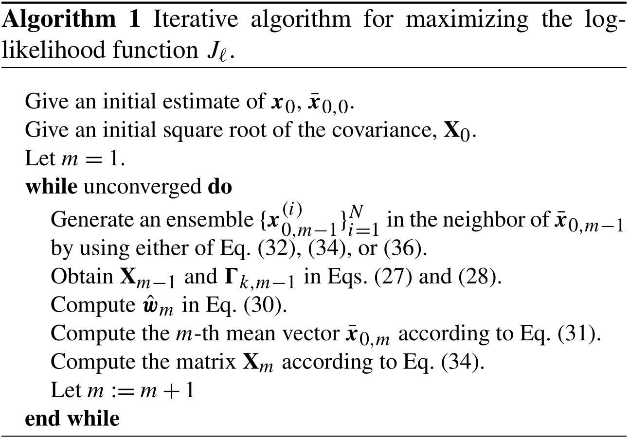
Equation (30) can be regarded as an approximation of the Levenberg–Marquardt method (e.g., Nocedal and Wright, 2006) for maximizing the log-likelihood function in Eq. (23) within the subspace spanned by . In particular, if is zero, Eq. (30) can be regarded as an approximation of the Gauss–Newton method. Indeed, Bocquet and Sakov (2013, 2014) derived a similar algorithm as an approximation of the Levenberg–Marquardt method or the Gauss–Newton method. However, the Levenberg–Marquardt method basically requires the Jacobian of the function gk, Gm−1. Since the above iterative algorithm does not directly use Gm−1, it would not be trivial to determine how the convergence of this algorithm is achieved. This issue is explored in this section.
We hereinafter assume that g(x0) is at least twice differentiable. The Taylor expansion up to the second-order term of Jℓ becomes the following:
where Gm−1 is the Jacobian at , and (∇2g) is a third-order tensor which consists of the Hessian matrix of each element of the vector-valued function g(x0). As in Eq. (12), we assume the following:
where Xm−1 is obtained by Eq. (27) given the ensemble . We then have the following:
In practical cases, the Jacobian matrix Gm−1 is typically unavailable. Ensemble variational methods thus employ the first-order approximation in Eq. 15 for ; that is, in the following:
where, in the following:
To evaluate this approximation when x0 has a large uncertainty, we consider the following expansion of g(x0) for each ensemble member :
If we consider a vector Γm−1wm, it becomes the following:
If , which is contained in the first-order term in Eq. (39), is approximated by Γm−1wm, then this means that the second- and higher-order terms of the right-hand side of Eq. (43) are neglected. Indeed, this can be justified if the spread of the ensemble is taken to be small. In our iterative scheme, the ensemble spread can be tuned freely. Even if the scale of is very small, any x0, which may have a large uncertainty, can be represented by taking the scale of to be large according to Eq. (38). The nonlinear terms of the right-hand side of Eq. (43) are of the order of , while they are of the order of or higher order. Thus, if the spread of the ensemble is taken to be small, the nonlinear terms of Eq. (43) would be suppressed, and we obtain the following:
Consequently, we can apply the approximation in Eq. (40) to Eq. (39). Defining a function as follows:
gives an approximation of in Eq. (39) as follows:
The fourth term on the right-hand side of Eq. (45) would not necessarily be suppressed, even if the ensemble variance were taken to be small, because it is of the order of and of the order of . To control the effect of this term, we introduce the idea of the minorize–maximize algorithm (MM algorithm; Lange et al., 2000; Lange, 2016). The MM algorithm is a class of iterative algorithms which considers a surrogate function which minorizes the objective function ϕ(z) and maximizes the surrogate function. Although the Levenberg–Marquardt method can also be regarded as an instance of the MM algorithm, the generic idea of the MM algorithm gives striking insight into the behavior of the algorithm.
At the mth step of the MM algorithm, the surrogate function, given the (m−1)th estimate zm−1, , is chosen to satisfy the following conditions:
The mth estimate, zm, is obtained by maximizing the mth surrogate function, . Since zm obviously satisfies the following:
it is guaranteed that the mth estimate is as good as or better than the (m−1)th estimate. After iterations, zm converges to a stationary point zs of the objective function ϕ(z) (Lange, 2016). If the Hessian matrix of ϕ(z) is negative definite in a neighborhood of zs, the stationary point zs becomes a local maximum (e.g., Nocedal and Wright, 2006). Therefore, the estimate would monotonically converge to a local maximum of ϕ(z) by repeating iterations if the following conditions are met:
-
the surrogate function ψ(z|zm) is twice differentiable and satisfies Eqs. (47a) and (47b),
-
and the Hessian of ϕ(z) is a negative definite in a neighborhood of the stationary point zs.
Here we consider the following surrogate function :
which is a similar treatment to Böhning and Lindsay (1988). For a given Δ, we can take so that the following inequality holds over :
where the equality holds if wm=0. If is chosen so that the inequality (50) is satisfied, satisfies the following:
This means that can be used as a surrogate function for maximizing according to the MM algorithm. Since Eq. (49) is the same as Eq. (29), the maximum of is achieved when where is given by Eq. (30). Obviously, satisfies the following inequality:
and therefore, if the approximation in Eq. (40) is valid, then we obtain the following result:
where is given by Eq. (31).
The above discussion is valid regardless of the choice of the ensemble in each iteration as far as the approximation in Eq. (40) is applicable. This suggests that we can use various ways to update the ensemble, including Eq. (36) which does not confine the ensemble within a particular subspace. It should be noted that the equality of Eq. (53) holds at a stationary point in the subspace spanned by the ensemble members. If the update of the ensemble in each iteration is carried out with Eq. (32) or (34), then the ensemble is confined within a particular subspace spanned by the initial ensemble, and would converge to a stationary point in this subspace. According to Eq. (37), if the nonlinearity of g is not severe when (∇2g) is not dominant, the Hessian of Jℓ is negative definite in a region where is small enough. This suggests that the iterative algorithm in Sect. 4 would attain at least a local maximum of Jℓ in the subspace for weakly nonlinear problems if Eq. (36) is applicable. If the ensemble is updated according to Eq. (36), a stationary point is sought in a different subspace in each iteration. If Qm is full rank, Jℓ would increase until a point which can be regarded as a stationary point in any N-dimensional subspace, and would thus converge to a local maximum in the full vector space after infinite iterations.
Based on the foregoing, convergence to a local maximum of the objective function Jℓ can be achieved for weakly nonlinear systems if the ensemble variance is taken to be small enough. If the ensemble with large spread is used, the estimate can be biased due to the nonlinear terms in Eq. (43). Hence, an ensemble with small spread would provide a satisfactory result for weakly nonlinear systems where we can assume the Hessian of Jℓ is a negative definite over the region of interest. However, this iterative algorithm does not necessarily guarantee convergence to the global maximum. If there are multiple peaks in Jℓ, it might be effectual to start with an ensemble with a large spread to approach the global maximum. An ensemble with a large spread would grasp a large-scale structure of the objective function because the ensemble approximation of the Jacobian gives the gradient averaged over the region where the ensemble members are distributed under a certain assumption (Raanes et al., 2019). Even if the spread is taken to be large at first, convergence would eventually be achieved by reducing the ensemble spread in each iteration, as described in the previous section.
Our formulation refers to the result of a simulation run initialized at the (m−1)th estimate for obtaining the mth estimate in Eq. (31). On the other hand, in many studies, the ensemble mean of simulation runs is used as a substitute for . If the ensemble mean is used, the ensemble in each iteration must be generated so as to satisfy Eq. (26), which is not required in our formulation; that is, the ensemble mean must be equal to the (m−1)th estimate . It should also be kept in mind that some bias due to the nonlinear terms in Eq. (42) could be introduced when the ensemble mean is used instead of . However, this bias could be suppressed by taking the ensemble spread to be small. Since the use of the ensemble mean would save the computational cost of one simulation run for each iteration, it might be a useful treatment for practical applications.
It is also important to appropriately choose the parameter . A sufficiently large guarantees that the mth estimate is better than the previous estimate , and hence, convergence is stable. However, convergence speed will be degraded with large because is strongly constrained by the penalty weighted with . Although there is no definitive way to determine this parameter, should have a similar scale to the right-hand side of Eq. (50); that is, if the third- and higher-order terms are assumed to be negligible then, in the following:
Since the right-hand side of Eq. (55) contains (∇2g) which comes from a nonlinear term of the function g, should be taken larger as system nonlinearity is more severe. This equation also suggests that should depend on the discrepancy between observation y and the (m−1)th prediction . Although (∇2g) is unknown in general, could be used as a guide for determining . The parameter should also be dependent on the variance of the ensemble. If an ensemble with a large spread is used, should be set as large accordingly.
The algorithm in Sect. 4 maximizes the log-likelihood function in Eq. (23). However, sometimes it would be required that prior information is incorporated into the estimate in a Bayesian manner. We thus consider the following log-posterior density function as the objective function:
which is the same as Eq. (10), although the vectors of the whole time sequence are combined into a single vector for each y and g(x0) as in Eq. (23). Equation (56) is proportional to the log-posterior distribution when p(x0) and p(y|x0) are assumed to be Gaussian. The Taylor expansion of Eq. (56) is as follows:
Applying Eqs. (38) and (44), we obtain the following approximate objective function:
As per Eq. (50), we can take so that the fifth and sixth terms on the right-hand side of Eq. (58) can be minorized by a quadratic function , and we obtain the following surrogate function which minorizes the function as follows:
which satisfies the following conditions:
This function is maximized when, in the following:
The mth estimate for x0 is obtained as follows:
Similar to Eq. (54), we obtain the following:
Thus, is a better estimate than if the approximation in Eq. (44) is valid. Generating the (m+1)th ensemble around , we can obtain the (m+1)th surrogate function according to Eq. (59) and proceed to the next iteration.
There are various methods for updating the ensemble including the methods mentioned in Sect. 4. Eq. (32) or (34) is convenient for practical problems because we can avoid computing the inverse of P0,b in Eq. (62). When Eq. (32) is used for updating the ensemble, we can easily avoid computing the inverse of P0,b by drawing initial ensemble members from the prior distribution . If initial ensemble members obey the prior distribution, we can use the same approximation as Eq. (13); that is, in the following:
Applying Eq. (63) recursively, can be reduced to the following:
Inserting Eqs. (32) and (66) into Eq. (62) and applying Eq. (65), we obtain the following:
Thus, we can avoid computing the inverse of P0,b. Likewise, when Eq. (34) is used for updating the ensemble, we can apply Eq. (65) to avoid computing the inverse of P0,b (See the Appendix).
As described in the previous section, the use of Eq. (32) of (34) confines the estimate within the subspace spanned by the initial ensemble. On the other hand, Eq. (36) enables us to seek the optimal value of x0 in a different subspace in each iteration. We can then obtain the local maximum in the full vector space if Qm is taken to be full rank. It appears that a similar approximation to Eq. (67) is applicable if Qm is taken to be a scalar matrix of P0,b. However, since this approximation considers a different approximate objective function in each iteration, monotonic convergence is not guaranteed. In order to ensure monotonic convergence, Eq. (36) requires the inverse of P0,b in general. Nonetheless, if can be obtained, the method with Eq. (36) would be helpful for improving the estimate.
Preceding studies have already demonstrated the usefulness of the ensemble-based iterative algorithms for various data assimilation problems. Estimation with the ensemble update in Eq. (32) has been verified in detail (e.g., Bocquet and Sakov, 2014). The iterative algorithm ensemble update in Eq. (34) has also been demonstrated (e.g., Minami et al., 2020). Although it might not be necessary to show the ability of the ensemble-based iterative algorithm further, we here verify some properties suggested in the above discussion through twin experiments with a simple model rather than a practical model.
In this section, we employ the Lorenz 96 model (Lorenz and Emanuel, 1998), which is written by the following equations:
for , where , x0=xM, and . The state dimension M was taken to be 40, and the forcing term f was taken to be 8. The true scenario was generated by running the model with a certain initial state. We here consider a weakly nonlinear problem. The assimilation window was accordingly taken as a short time interval . It was assumed that all the state variables could be observed with a fixed time interval (Δt=0.1), and hence, 80 data were generated for each state variable. The observation noise for each variable was assumed to independently follow a Gaussian distribution with mean 0 and standard deviation 0.5. In each data assimilation experiment, the prior distribution was assumed to be a Gaussian distribution with mean 0 and variance ζ2I, 𝒩(0,ζ2I), where ζ=5.
We compare two ensemble updating methods of Eqs. (32) and (36). In applying Eq. (32), the initial ensemble was drawn from a Gaussian distribution 𝒩(0,ε2I), where and X0 was obtained as follows:
The matrix Xm for each iteration was fixed at Xm=X0, which corresponds to the setting in Eq. (32) with αm=1. The discussion in Sect. 5 suggests that the penalty parameter should be determined according to Eq. (55). Although (∇2g) is unknown, we can say that should be related with the variance of the ensemble and the discrepancy between y and . We thus gave as follows:
where we tried two cases with and . Here the part of the square root of a quadratic form of was multiplied in order that was roughly proportional to , and was for representing the variance of the ensemble.
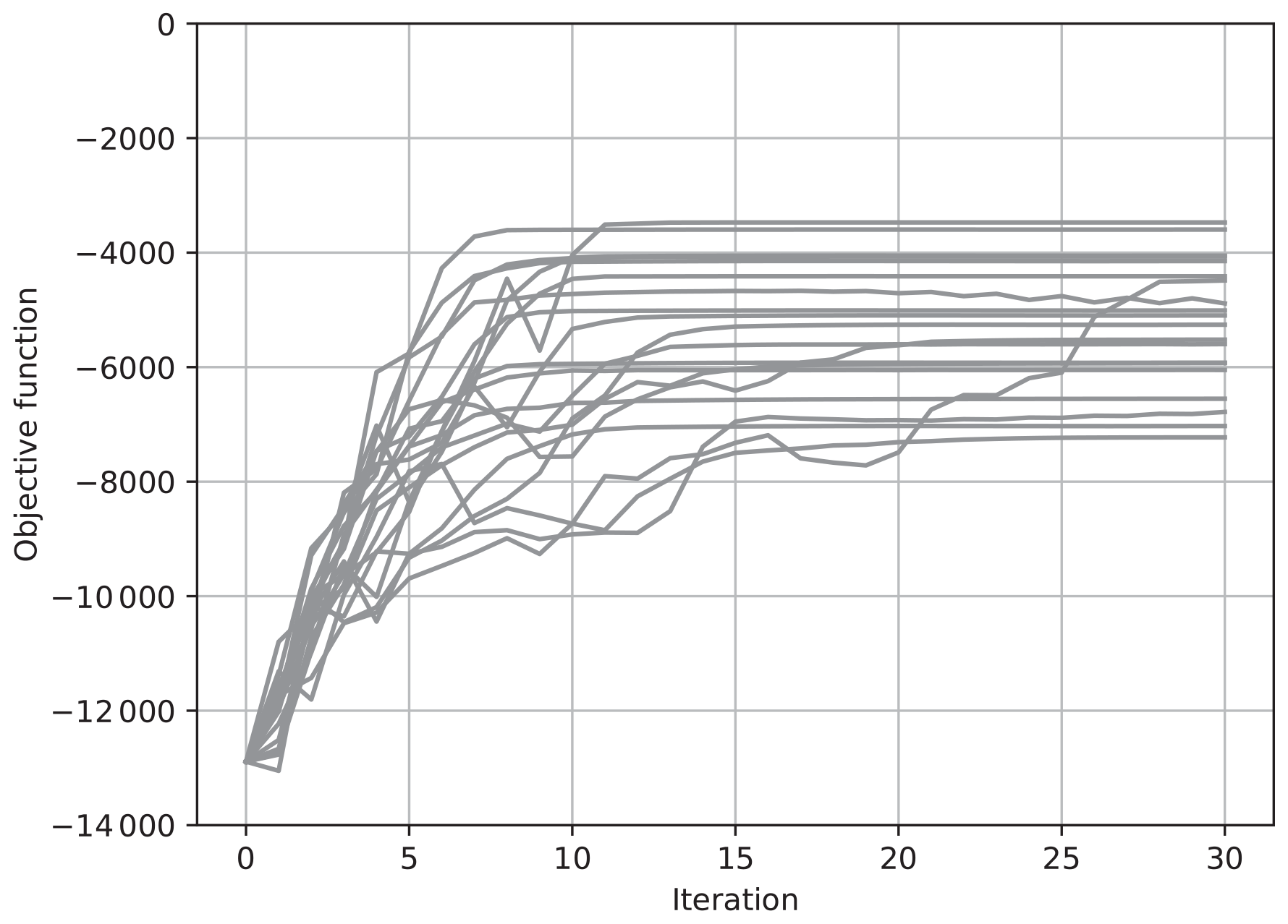
Figure 1The value of the objective function J for each iteration for 20 trials of the estimation. The ensemble was updated using Eq. (32) with .
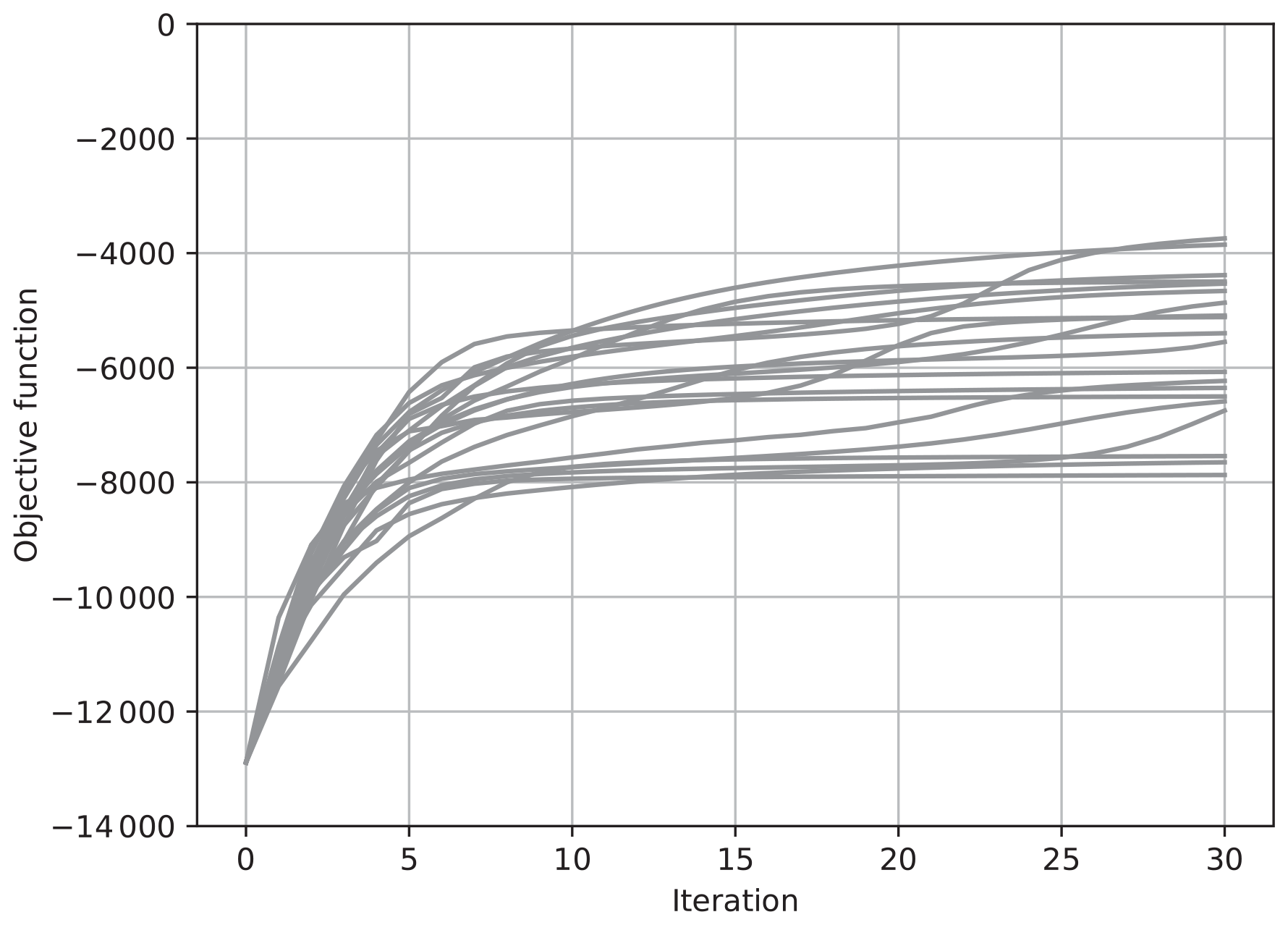
Figure 2The value of the objective function J for each iteration for 20 trials of the estimation. The ensemble was updated using Eq. (32) with .
Figures 1 and 2 show results with Eq. (32), where and , respectively. We took the ensemble size N to be 30, which is less than the state dimension, and performed the estimation 20 times with different seeds of a pseudo random number generator. The value of the objective function J in Eq. (56) for each iteration is plotted for each of 20 trials in these figures. When , the value of J tended to increase more sharply than when . However, J did not monotonically increase when , while it monotonically increased when . According to the discussion in Sect. 5, monotonic convergence is achieved when is taken to be large enough. However, convergence speed becomes slow when is large. The results in Figs. 1 and 2 thus confirmed our discussion on the convergence. However, the results shown in Figs. 1 and 2 did not converge to the same value, which means the results depended on the seeds of pseudo random numbers. This would indicate that a local maximum within a subspace spanned by the ensemble does not match the maximum in the full state vector space, and that the value of the local maximum depends on the subspace.
Figures 3 and 4 show results with Eq. (36), where and , respectively. Again, the ensemble size N was taken to be 30, and the results of 20 trials with different seeds of pseudo random numbers are overplotted. Again, when , the increase in J tended to be sharp, while it was not monotonic. On the other hand, when , the increase in J was gradual but monotonic. In contrast with the results in Figs. 3 and 4, the values of J in different trials converged to the same value after about 15 iterations, as in the case with shown in Fig. 3. In the case with , the convergence was much slower, but the values of J converged to the same value as the case with after about 80 iterations in all of the 20 trials (not shown). These results show that the maximum of the objective function in the full vector space can be reached by changing an ensemble in each iteration even if the ensemble does not span the full vector space.
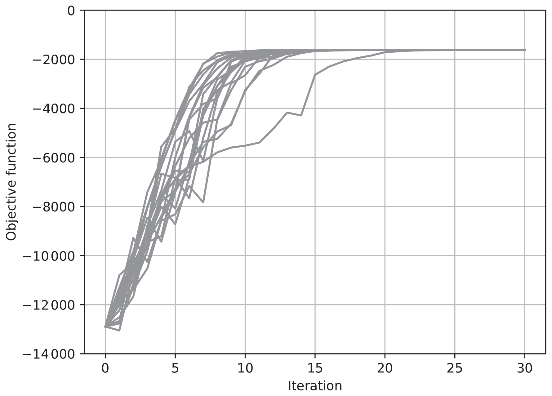
Figure 3The value of the objective function J for each iteration for 20 trials of the estimation. The ensemble was updated using Eq. (36) with .
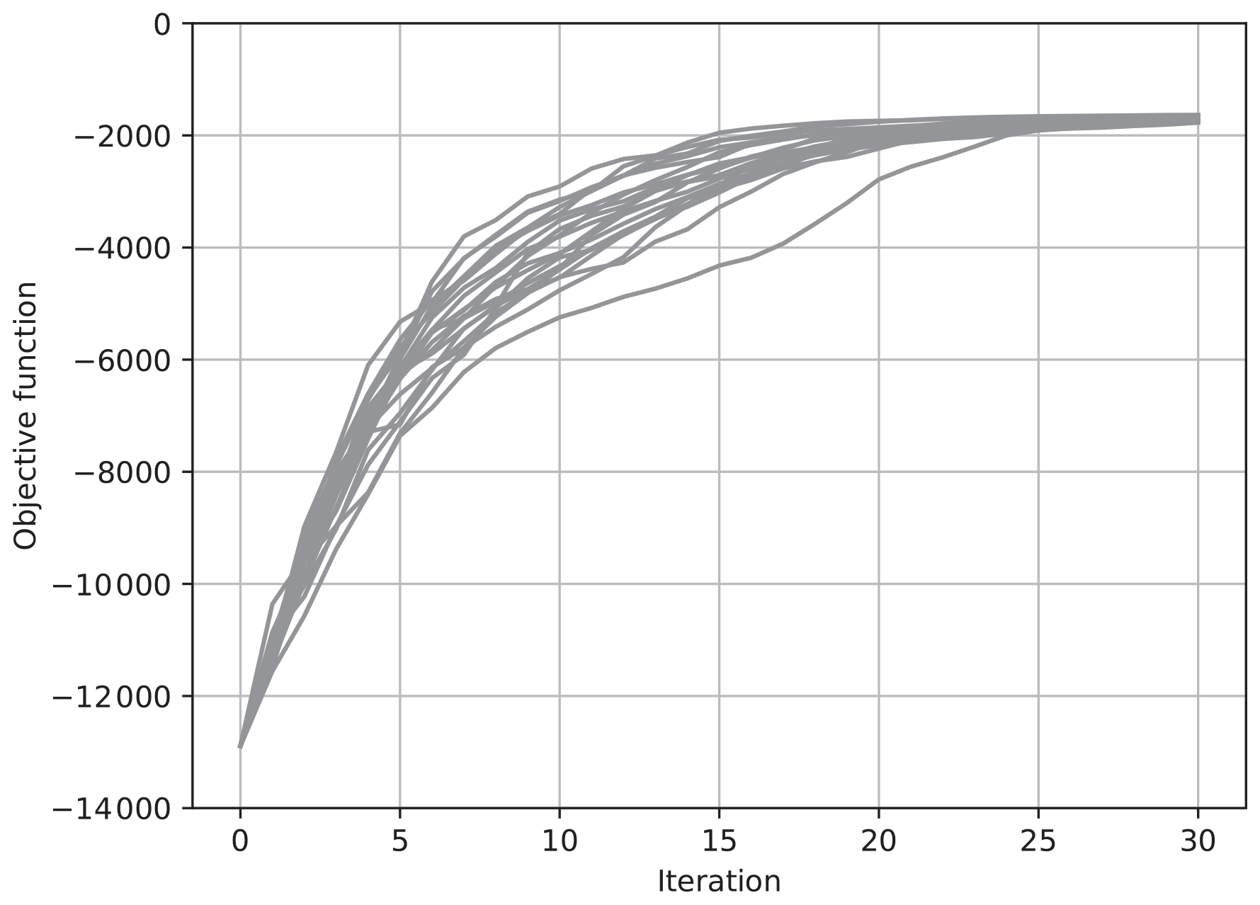
Figure 4The value of the objective function J for each iteration for 20 trials of the estimation. The ensemble was updated using Eq. (36) with .
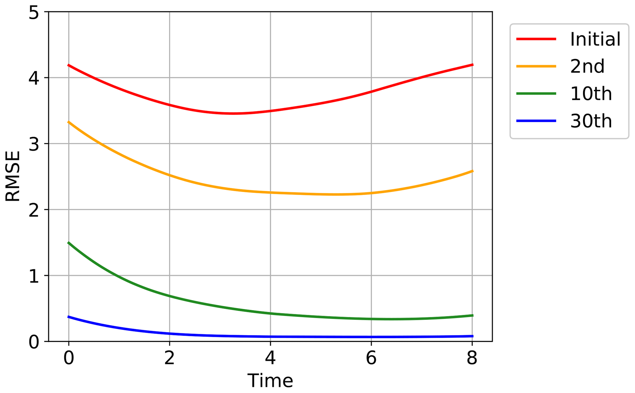
Figure 5 shows the convergence of the estimated time series to the true time series for one of the 40 state variables, x1, in one of the 20 trials in Fig. 4. The red line indicates the initial guess obtained by running the Lorenz 96 model started at . The yellow, green, and blue lines show the estimates after the second, 10th, and 30th iterations, respectively. The truth is indicated with the gray line, and the time series of the synthetic observations used in this experiment are overplotted with gray dots. Although the initial trajectory (red line) showed was obviously dissimilar to the true trajectory (gray line), the estimate was improved by repeating the iterations as also shown in Fig. 4. After 30 iterations, the estimate was very close to the truth, and the temporal evolution was well reproduced. Figure 6 shows the root mean square errors of the estimates, which means the root mean squares of the differences between the estimates and the true values over all the 40 variables at each time step in the same trial as in Fig. 5. Again, the red line indicates the initial guess, and the yellow, green, and blue lines show the estimates after the second, 10th, and 30th iterations, respectively. The errors were certainly reduced over the period of the assimilation by the iterations.
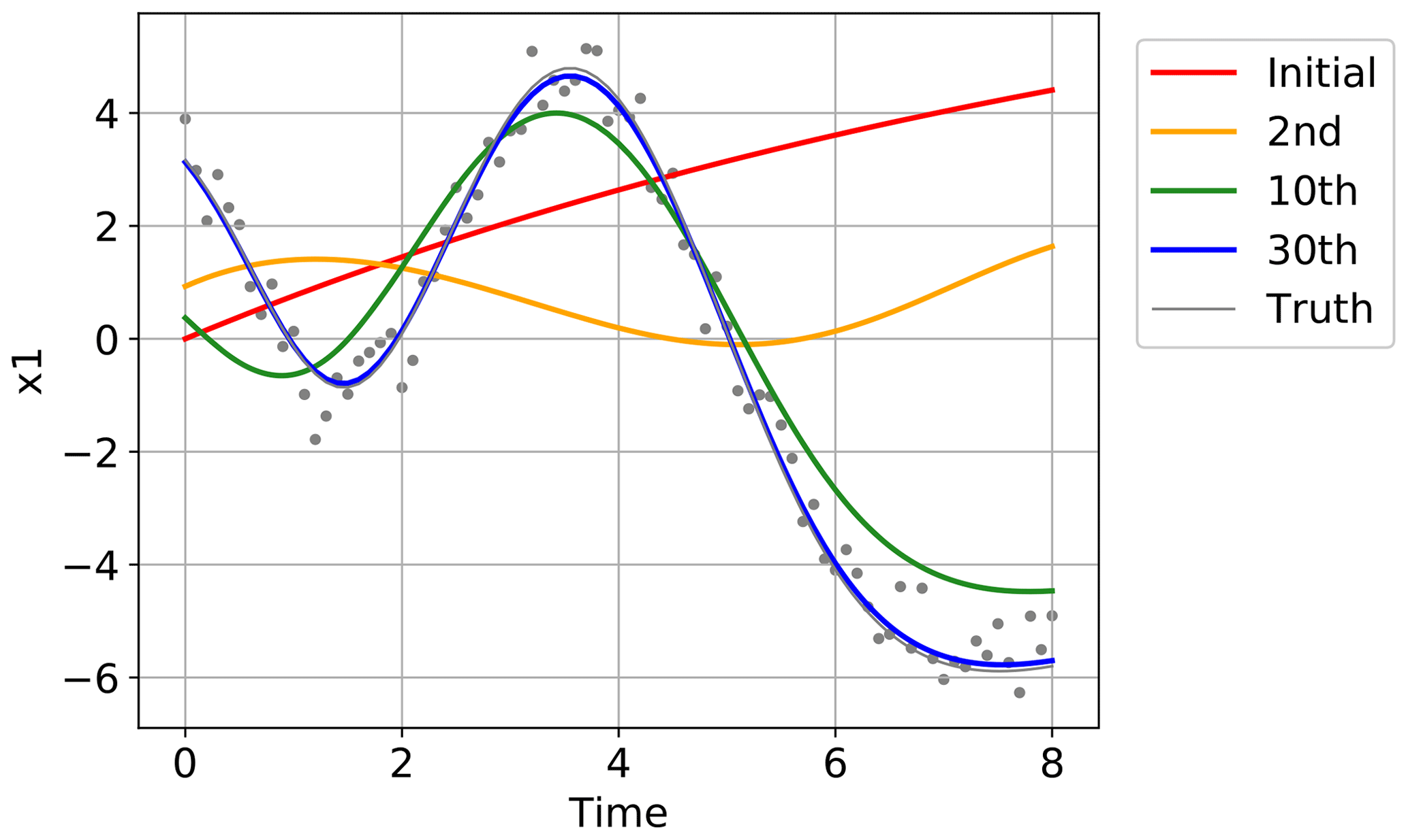
Figure 5The temporal evolution started at the initial guess (red line), and the estimated evolutions after the second (yellow line), 10th (green line), and 30th iterations (blue line) in one of the 20 trials in Fig. 4. The truth is indicated with the gray line, and the time series of the synthetic observations used in this experiment are overplotted with gray dots.
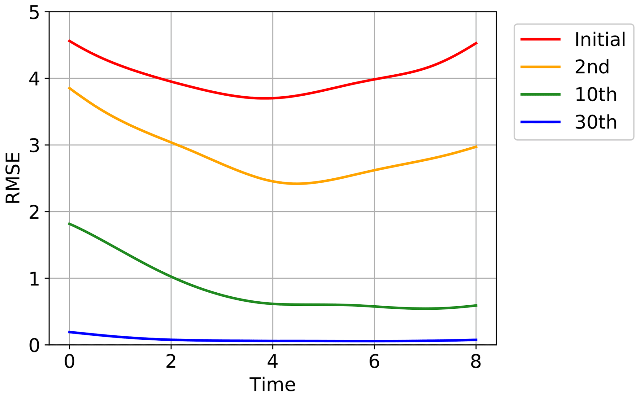
Figure 6The root mean square errors over all the 40 variables at each time step for the initial guess (red line), the second iteration (yellow line), the 10th iteration (green line), and the 30th iteration (blue line) in the same trial as Fig. 5.
In order to closely investigate the effect of , we conducted additional experiments for a case in which nonlinearity is a little stronger. While Figs. 3 and 4 show the results when the assimilation window was taken as , Figs. 7 and 8 show the results with a little longer assimilation window, . Although the other settings were the same as Figs. 3 and 4, the effect of the nonlinearity on the objective function J was a little more severe due to the longer assimilation window. When , the J value converged to about −2000 in many of the 20 trials. In some trials, however, J did not converge but oscillated below −6000. In contrast, when δ was as large as , the J value converged to the same value after about 50 iterations in all of the 20 trials. As discussed in Sect. 5, a sufficiently large guarantees that the estimate is improved in each iteration. Although the convergence speed becomes worse, a stable estimation can be attained.

Figure 7The value of the objective function J for each iteration for 20 trials of the estimation. The ensemble was updated using Eq. (36) with , and the ensemble window was taken as .
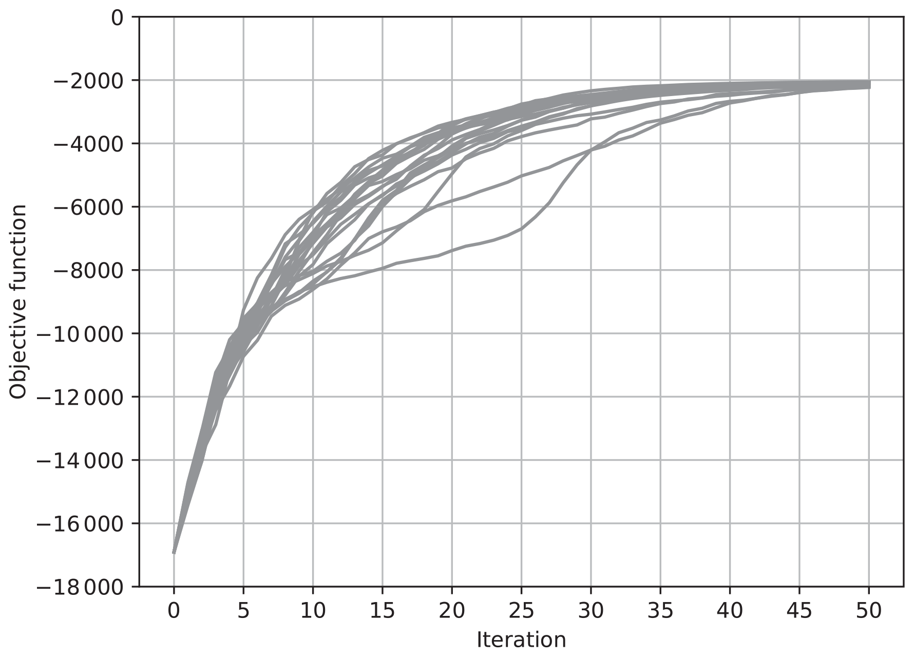
Figure 8The value of the objective function J for each iteration for 20 trials of the estimation. The ensemble was updated using Eq. (36) with , and the ensemble window was taken as .
We also conducted experiments with a higher-dimensional system. The method with a randomly generated ensemble was applied to the Lorenz 96 model with 400 variables (M=400), of which the dimension is 10 times higher. Figure 9 shows the result with 400 variables. The assimilation was taken as , and δ was set at , which is the same as the result in Fig. 3. The ensemble size N was taken to be 200. For the assimilation into the Lorenz 96 model with 400 variables, the convergence was attained in about 20 iterations with 200 ensemble members. In this high-dimensional case, monotonic convergence was achieved even if δ was taken to be as small as in Fig. 3. As far as we conducted experiments with the Lorenz 96 model with various dimensions, the convergence becomes stabler as the state dimension M becomes higher. This might imply that the nonlinear term (the fifth term of the right-hand side of Eq. 58) is depressed in the high-dimensional Lorenz 96 models. However, we have not resolved the reason for the stable convergence for the high-dimensional Lorenz 96 systems at present.
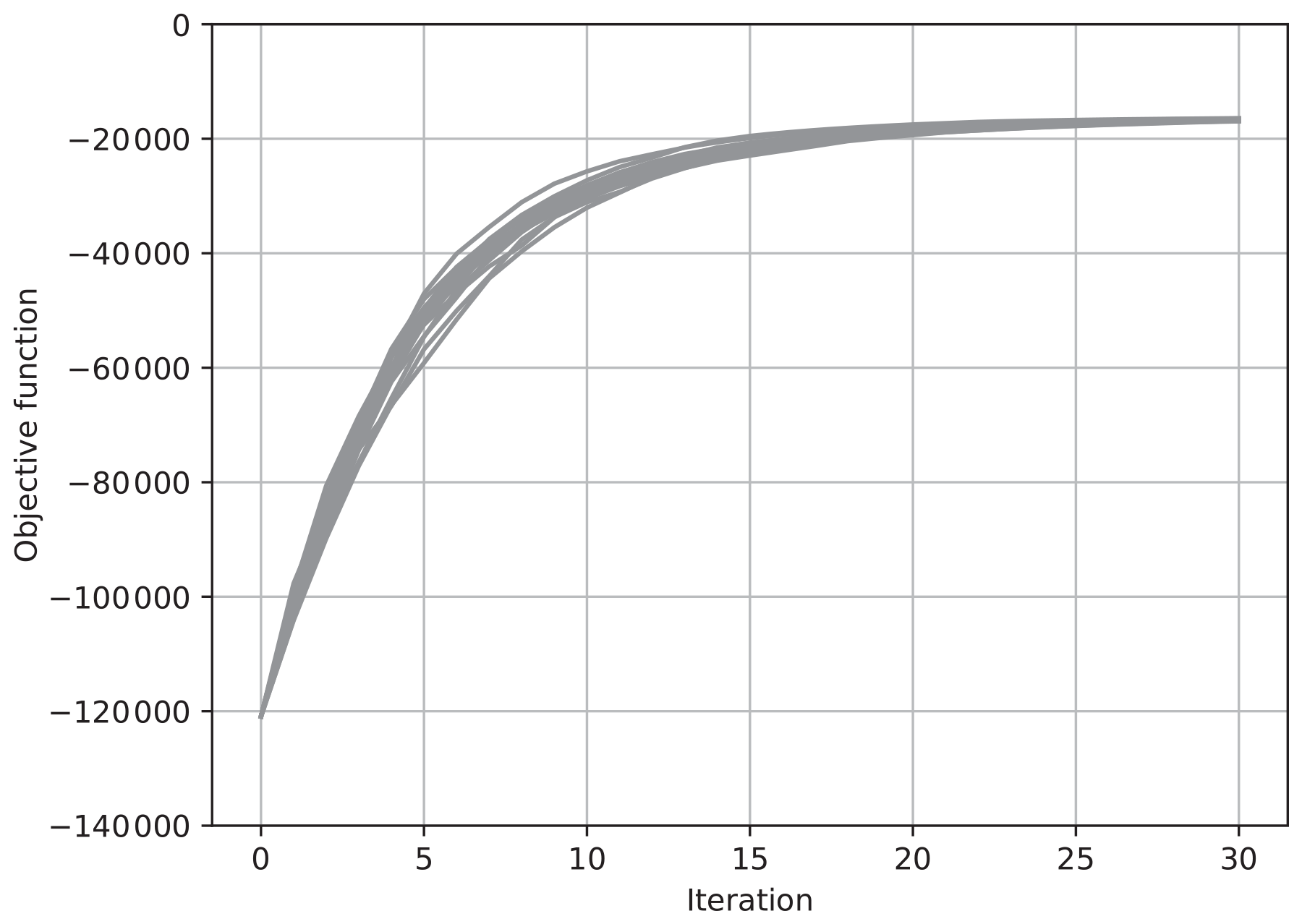
Figure 9The value of the objective function J for each iteration for 20 trials of the estimation for the 400 dimensional system. The ensemble was updated using Eq. (36) with .
In Fig. 10, we confirmed the convergence of the estimated time series to the true trajectory for one of the 400 state variables, x1, in one of the 20 trials in Fig. 9. The red line indicates the initial guess started at , and the yellow, green, and blue lines shows the estimates after the second, 10th, and 30th iterations, respectively. The gray line shows the truth, and the gray dots show the synthetic observations used in this experiment. Similar to Fig. 5, the estimate approached to the truth by repeating the iterations even in this high-dimensional case, and the true evolution was well reproduced after 30 iterations. In Fig. 11, the root mean square errors over all the 400 variables at each time step are in the same trial as Fig. 10. Each color corresponds to the respective iteration shown in Fig. 10. It is confirmed that the errors decreased over the period of the assimilation after repeating the iterations.
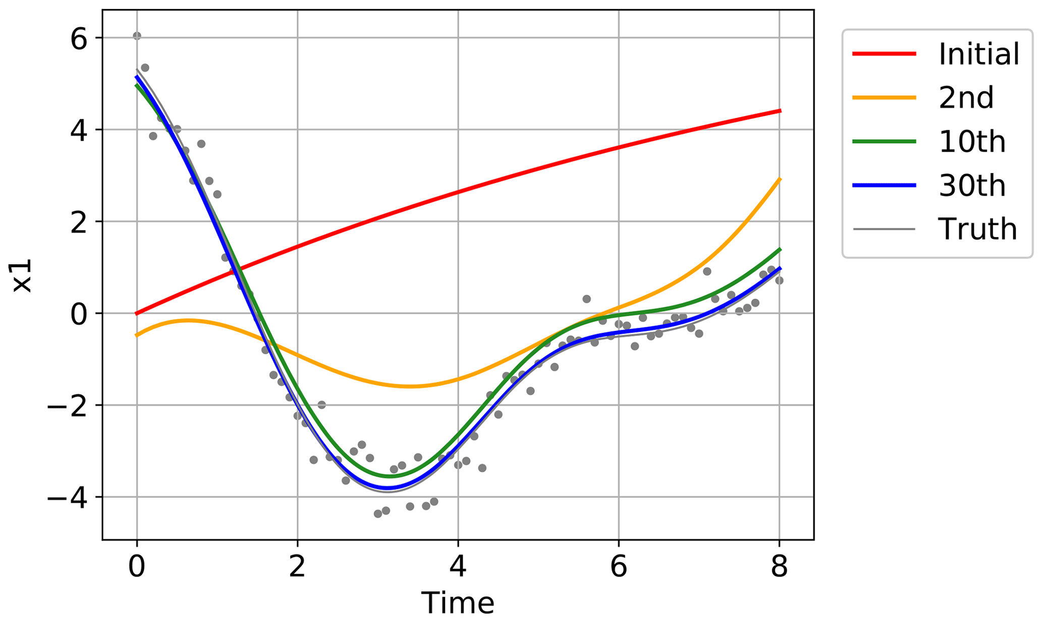
Figure 10The temporal evolution started at the initial guess (red line), and the estimated evolutions at the second (yellow line), 10th (green line), and 30th iterations (blue line) in one of the 20 trials in Fig. 9. The truth is indicated with the gray line, and the time series of the synthetic observations used in this experiment are overplotted with gray dots.
The ensemble variational method is derived under the assumption that a linear approximation of a dynamical system model is valid over a range of uncertainty. This linear approximation is not valid in such problems where the scale of uncertainty is much larger than the range of linearity. However, a local maximum of the log-likelihood or log-posterior function can be attained by updating the ensemble iteratively – even in cases with a large uncertainty. The present paper assessed the influence of system nonlinearity on this iterative algorithm after considering the nonlinear terms of the system function g. The discussion suggests two points to guarantee the monotonic convergence to a local maximum in the subspace spanned by the ensemble. One is that the ensemble spread must be set to be small, and the other is that the penalty parameter must be set to be large enough. A sufficiently large would ensure monotonic convergence, although convergence speed would become poorer with too large a . The effect of this penalty term has also been experimentally confirmed in Sect. 7. These properties would be reasonable if this iterative algorithm is regarded as an approximation of the Levenberg–Marquardt method.
In applying the iterative algorithm discussed in this paper, the choice of the parameter would be an important issue. Although it was determined according to Eq. (70) in Sect. 7, Eq. (70) still requires tuning of the parameter δ. However, it is not necessary to finely tune δ because δ would not have a crucial effect on the performance of the algorithm. It would thus be enough to roughly determine δ. In addition, one could check whether the objective function J increases or not at each iteration just by running one forward simulation initialized at . In the iterative algorithm, the most computational cost is spent on running the ensemble simulation with multiple initial states. The pilot run, which is computationally much cheaper than the ensemble run, would be a feasible way of tuning δ in practical cases.
One issue peculiar to the ensemble-based method is the rank deficiency, which occurs when the ensemble size is smaller than the dimension of the initial state x0. If the ensemble is confined within a particular subspace, the iterative algorithm can only attain the optimal value within the subspace spanned by the ensemble. However, our discussion indicates that, if is sufficiently large, then it is ensured that the discrepancies between estimates and observations are reduced in each iteration – even if the ensemble is confined within a subspace. If the ensemble is updated so as to span a different subspace in each iteration, as indicated in Eq. (36), the optimal solution would be sought in a different subspace in each iteration, and the estimate would converge to a local maximum in the full vector space after infinite iterations. It should be noted that this paper has not assessed how well the method with a random ensemble generation with Eq. (36) works in practical high-dimensional problems, although it is, in theory, applicable as far as the inverse of P0,b is available. Further research would be required to clarify its performance in high-dimensional geophysical models in order to reinforce this study.
Compared with the adjoint method, which is a conventional variational method for 4D variational problems, the convergence rate of this iterative method would be poorer because it employs an ensemble approximation within a lower-dimensional subspace at each iteration. Nonetheless, we can say that the iterative ensemble-based method is potentially useful because it is much easier to implement. While the adjoint method requires an adjoint code which is usually time-consuming to develop, the ensemble-based method can solve the same problem without requiring an adjoint code. This paper mainly considers data assimilation problems. However, the framework of the iterative ensemble variational method is also applicable to general nonlinear inverse problems as far as the Gaussian assumption in Eq. (23) or Eq. (56) is upheld. If an ensemble of the results of forward runs is available, many practical problems can readily be addressed. This method could therefore be a promising tool for data assimilation and various inverse problems.
In the following, it is described how the iteration can be performed without computing the inverse of P0,b when the ensemble is updated with the ensemble transform scheme in Eq. (34). When the ensemble is updated by the ensemble transform in the manner of Eq. (34) as follows:
the transform matrix Tm should be given as follows:
where Um and Λm are obtained by the following eigenvalue decomposition:
If Xm−1 is obtained according to Eq. (A1), as follows:
Defining the matrix Cm−1 as follows:
Xm−1 can be written as follows:
If the initial ensemble is sampled from the prior distribution , then we can apply Eq. (65) again. Using Eqs. (65) and (A6), the term in Eq. (62) can be reduced to the following:
The mth estimate is broken down as follows:
where C0=I. Defining a vector ξm−1 is as follows:
then Eq. (A8) becomes the following:
and we obtain the following:
Using Eqs. (65) and (A11), we can rewrite Eq. (62) into a form without the inverse of P0,b as follows:
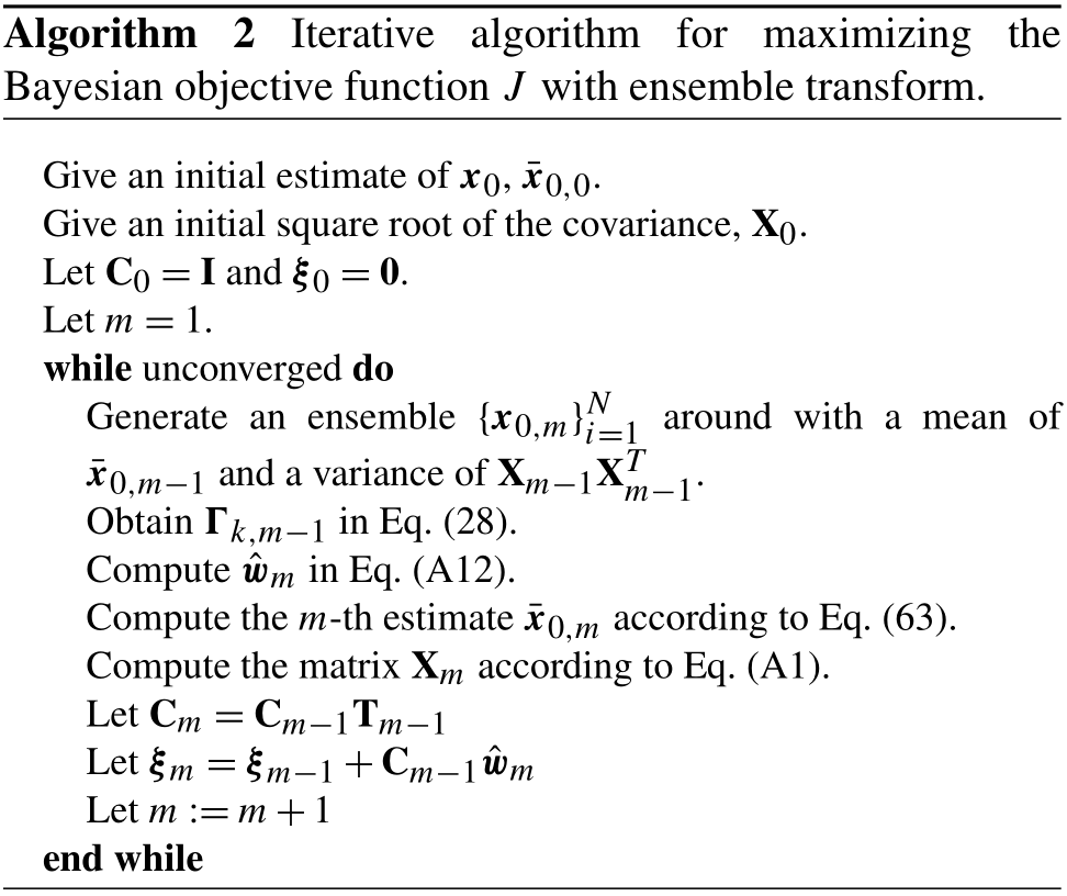
The algorithm with the ensemble transform is summarized in Algorithm 2.
The code for reproducing the experimental results shown in Sect. 7 is archived on Zenodo (https://doi.org/10.5281/zenodo.4420875; Nakano, 2020).
The author declares that there is no conflict of interest.
This research has been supported by the Japan Society for the Promotion of Science (grant no. 17H01704) and by PRC JSPS CNRS, the Bilateral Joint Research Project “Forecasting the geomagnetic secular variation based on data assimilation”.
This paper was edited by Amit Apte and reviewed by three anonymous referees.
Bannister, R. N.: A review of operational methods of variational and ensemble-variational data assimilation, Q. J. Roy. Meteor. Soc., 143, 607–633, https://doi.org/10.1002/qj.2982, 2017. a
Bishop, C. H., Etherton, B. J., and Majumdar, S. J.: Adaptive sampling with the ensemble transform Kalman filter. Part I: Theoretical aspects, Mon. Weather Rev., 129, 420–436, 2001. a
Bocquet, M. and Sakov, P.: Combining inflation-free and iterative ensemble Kalman filters for strongly nonlinear systems, Nonlin. Processes Geophys., 19, 383–399, https://doi.org/10.5194/npg-19-383-2012, 2012. a
Bocquet, M. and Sakov, P.: Joint state and parameter estimation with an iterative ensemble Kalman smoother, Nonlin. Processes Geophys., 20, 803–818, https://doi.org/10.5194/npg-20-803-2013, 2013. a, b, c, d
Bocquet, M. and Sakov, P.: An iterative ensemble Kalman smoother, Q. J. Roy. Meteor. Soc., 140, 1521–1535, https://doi.org/10.1002/qj.2236, 2014. a, b, c, d
Böhning, D. and Lindsay, B. G.: Monotonicity of quadratic-approximation algorithms, Ann. Inst. Statist. Math., 40, 641–663, 1988. a
Buehner, M.: Ensemble-derived stationary and flow-dependent background-error covariances: Evaluation in a quasi-operational NWP setting, Q. J. Roy. Meteor. Soc., 131, 1013–1043, 2005. a, b
Buehner, M., Houtekamer, P. L., Charette, C., Mitchell, H. L., and He, B.: Intercomparison of variational data assimilation and the ensemble Kalman filter for global deterministic NWP. Part I: Description and single-observation experiment, Mon. Weather Rev., 138, 1550–1566, 2010. a, b
Chen, Y. and Oliver, D. S.: Ensemble randomized maximum likelihood method as an iterative ensemble smoother, Math. Geosci., 44, 1–26, 2012. a
Courtier, P., Thépaut, J.-N., and Hollingsworth, A.: A strategy for operational implementation of 4D-Var, using an incremental approach, Q. J. Roy. Meteor. Soc., 120, 1367–1387, 1994. a
Emerick, A. A. and Reynolds, A. C.: History matching time-lapse seismic data using the ensemble Kalman filter with multiple data assimilation, Computat. Geosci., 16, 639–659, https://doi.org/10.1007/s10596-012-9275-5, 2012. a
Emerick, A. A. and Reynolds, A. C.: Ensemble smoother with multiple data assimilation, Computers Geosci., 55, 3–15, https://doi.org/10.1016/j.cageo.2012.03.011, 2013. a
Evensen, G.: Analysis of iterative ensemble smoothers for solving inverse problems, Computat. Geosci., 22, 885–908, https://doi.org/10.1007/s10596-018-9731-y, 2018. a
Evensen, G. and van Leeuwen, P. J.: An emsemble Kalman smoother for nonlinear dynamics, Mon. Weather Rev., 128, 1852–1867, 2000. a
Godinez, H. C., Yu, Y., Lawrence, E., Henderson, M. G., Larsen, B., and Jordanova, V. K.: Ring current pressure estimation with RAM-SCB using data assimilation and Van Allen Probe flux data, Geophys. Res. Lett., 43, 11948–11956, https://doi.org/10.1002/2016GL071646, 2016. a
Gu, Y. and Oliver, D. S.: An iterative ensemble Kalman filter for multiphase fluid flow data assimilation, SPE J., 12, 438–446, 2007. a
Kalnay, E. and Yang, S.-C.: Accelerating the spin-up of ensemble Kalman filtering, Q. J. Roy. Meteor. Soc., 136, 1644–1651, 2010. a
Kano, M., Miyazaki, S., Ishikawa, Y., Hiyoshi, Y., Ito, K., and Hirahara, K.: Real data assimilation for optimization of frictional parameters and prediction of afterslip in the 2003 Tokachi-oki earthquake inferred from slip velocity by an adjoint method, Geophys. J. Int., 203, 646–663, https://doi.org/10.1093/gji/ggv289, 2015. a
Lange, K.: MM optimization algorithms, Society for Industrial and Applied Mathematics, Philadelphia, USA, 2016. a, b
Lange, K., Hunter, D. R., and Yang, I.: Optimization transfer using surrogate objective functions, J. Comput. Graph. Statist., 9, 1–20, 2000. a
Lawless, A. S., Gratton, S., and Nichols, N. K.: An investigation of incremental 4D-Var using non-tangent linear model, Q. J. Roy. Meteor. Soc., 131, 459–476, 2005. a
Liu, C., Xiao, Q., and Wang, B.: An ensemble-based four-dimensional variational data assimilation scheme. Part I: Technical formulation and preliminary test, Mon. Weather Rev., 136, 3363–3373, 2008. a, b
Liu, C., Xiao, Q., and Wang, B.: An ensemble-based four-dimensional variational data assimilation scheme. Part II: Observing system simulation experiments with advanced research WRF (ARW), Mon. Weather Rev., 137, 1687–1704, 2009. a, b
Livings, D. M., Dance, S. L., and Nichols, N. K.: Unbiased ensemble square root filters, Physica D, 237, 1021–1028, 2008. a
Lorenc, A. C.: The potential of the ensemble Kalman filter for NWP–a comparison with 4D-Var, Q. J. Roy. Meteor. Soc., 129, 3183–3203, 2003. a
Lorenz, E. N. and Emanuel, K. A.: Optimal sites for supplementary weather observations: Simulations with a small model, J. Atmos. Sci., 55, 399–414, 1998. a
Minami, T., Nakano, S., Lesur, V., Takahashi, F., Matsushima, M., Shimizu, H., Nakashima, R., Taniguchi, H., and Toh, H.: A candidate secular variation model for IGRF-13 based on MHD dynamo simulation and 4DEnVar data assimilation, Earth Planet. Space, 72, 136, https://doi.org/10.1186/s40623-020-01253-8, 2020. a, b, c
Nakano, S.: Experimental demonstration of the iterative ensemble-based variational method, Zenodo, https://doi.org/10.5281/zenodo.4420875, 2020. a
Nakano, S., Ueno, G., Ebihara, Y., Fok, M.-C., Ohtani, S., Brandt, P. C., Mitchell, D. G., Keika, K., and Higuchi, T.: A method for estimating the ring current structure and the electric potential distribution using ENA data assimilation, J. Geophys. Res., 113, A05208, https://doi.org/10.1029/2006JA011853, 2008. a
Nocedal, J. and Wright, S. J.: Numerical optimization, 2nd ed., Springer, New York, USA, 2006. a, b
Raanes, P. N., Stordal, A. S., and Evensen, G.: Revising the stochastic iterative ensemble smoother, Nonlin. Processes Geophys., 26, 325–338, https://doi.org/10.5194/npg-26-325-2019, 2019. a, b
Sanchez, S., Wicht, J., Bärenzung, J., and Holschneider, M.: Sequential assimilation of geomagnetic observations: perspectives for the reconstruction and prediction of core dynamics, Geophys. J. Int., 217, 1434–1450, https://doi.org/10.1093/gji/ggz090, 2019. a
van Leeuwen, P. J. and Evensen, G.: Data assimilation and inverse methods in terms of a probabilistic formulation, Mon. Weather Rev., 124, 2898–2913, 1996. a
Yokota, S., Kunii, M., Aonashi, K., and Origuchi, S.: Comparison between four-dimensional LETKF and emsemble-based variational data assimilation with observation localization, SOLA, 12, 80–85, https://doi.org/10.2151/sola.2016-019, 2016. a, b
Zupanski, M., Navon, M., and Zupanski, D.: The Maximum likelihood ensemble filter as a non-differentiable minimization algorithm, Q. J. Roy. Meteor. Soc., 134, 1039–1050, 2008. a
- Abstract
- Introduction
- The 4D variational data assimilation (4DEnVar)
- Ensemble-based method
- Iterative algorithm
- Rationale of the algorithm
- Bayesian form
- Experiments
- Discussion and conclusions
- Appendix A: Algorithm for Bayesian estimation with ensemble transform
- Code availability
- Competing interests
- Financial support
- Review statement
- References