Brief communication: Lower-bound estimates for residence time of energy in the atmospheres of Venus, Mars and Titan

The residence time of energy in a planetary atmosphere, τ, which was recently introduced and computed for the Earth's atmosphere (Osácar et al., 2020), is here extended to the atmospheres of Venus, Mars and Titan. τ is the timescale for the energy transport across the atmosphere. In the cases of Venus, Mars and Titan, these computations are lower bounds due to a lack of some energy data. If the analogy between τ and the solar Kelvin–Helmholtz scale is assumed, then τ would also be the time the atmosphere needs to return to equilibrium after a global thermal perturbation.

1 Introduction

When the inflow, ℱ_i, of any substance into a box is equal to the outflow, ℱ_o, then the amount of that substance in the box, ℳ, is constant. This constitutes an equilibrium or steady state. Then, the ratio of the stock in the box to the flow rate (in or out) is called residence time and is a timescale for the transport of the substance in the box.

$$\begin{array}{}\text{(1)}& t={\displaystyle \frac{\mathcal{M}}{\mathcal{F}}}.\end{array}$$

In Eq. (1) it is assumed that the substance is conserved. A good example of this type is the parameter defined in atmospheric chemistry (Hobbs, 2000) as the average residence time of each individual gas, defined as Eq. (1). ℳ is the total average mass of the gas in the atmosphere, and ℱ is the total average influx or outflux, which in time average for the whole atmosphere are equal.

In this work we extend the substance that flows in the box from matter to energy, and the residence time is

$$\begin{array}{}\text{(2)}& \mathit{\tau }={\displaystyle \frac{E}{F}},\end{array}$$

where E is the total energy in the box (a planetary atmosphere), and F is the energy flux that enters or leaves it.

Here, by using Eq. (2), we estimate the average residence time of energy in several planetary atmospheres. Planetary atmospheres constitute steady-state problems, because the storage of energy in their interior is not systematically increasing or decreasing. Several authors have previously considered the energy–residence-time relation in other types of problems (Mcilveen, 1992, 2010; Harte, 1988).

The structure of this communication is the following: Sect. 2 addresses the numerator of Eq. (2) E, while Sect. 3 deals with the denominator F. In Sect. 4 the residence time of energy is considered for the Sun. The paper concludes with a discussion (Sect. 5).

2 Forms of energy in a planetary atmosphere

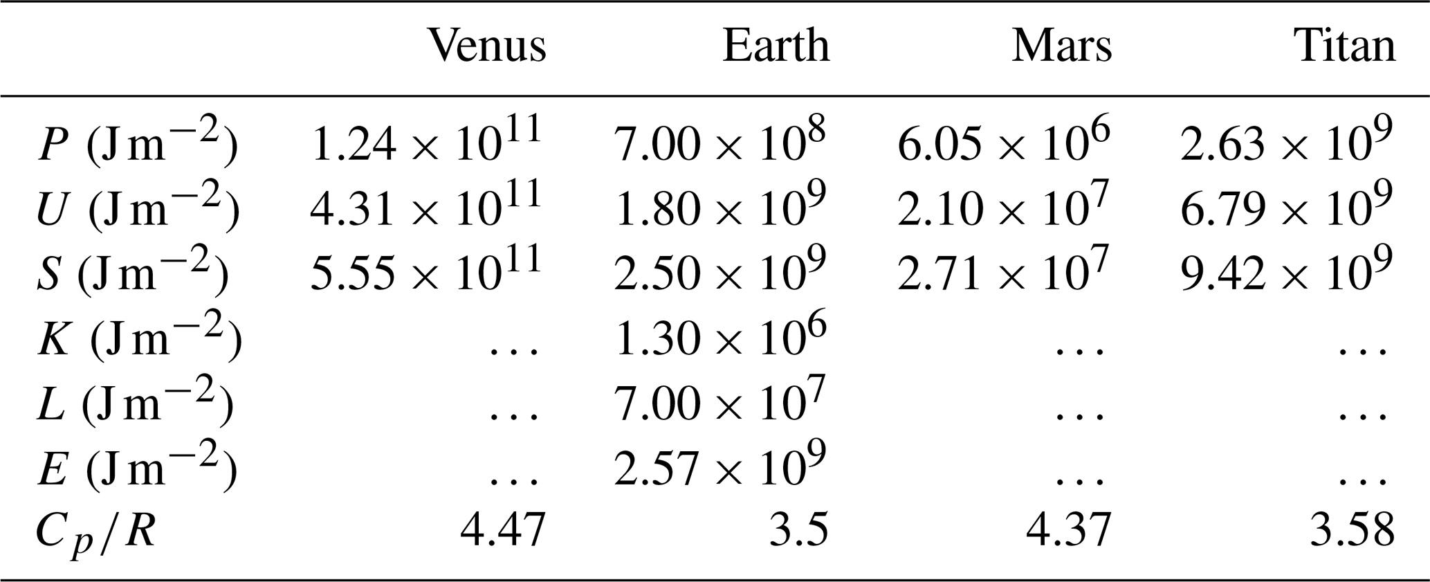
The most important forms of energy in an atmosphere are the thermodynamic internal energy, U; the potential energy due to the planet's gravity, P; the kinetic energy, K; and the latent energy, L, related to the phase transitions.

In a planar atmosphere, in hydrostatic equilibrium and by using the state equation for an ideal gas, the first two quantities can be written as

$$\begin{array}{}\text{(3)}& {\displaystyle }U=\underset{\mathrm{0}}{\overset{\mathrm{\infty }}{\int }}{c}_{\mathrm{v}}T\left(z\right)\mathit{\rho }\left(z\right)\mathrm{d}z={\displaystyle \frac{c_{\mathrm{v}}}{R}}\underset{\mathrm{0}}{\overset{\mathrm{\infty }}{\int }}p\left(z\right)\mathrm{d}z,\text{(4)}& {\displaystyle }P=\underset{\mathrm{0}}{\overset{\mathrm{\infty }}{\int }}gz\mathit{\rho }\left(z\right)\mathrm{d}z=\underset{\mathrm{0}}{\overset{\mathrm{\infty }}{\int }}p\left(z\right)\mathrm{d}z,\end{array}$$

In Eqs. (3) and (4), c_v is the specific heat at constant volume, R is the gas constant, and ρ(z) and T(z) are the density and temperature of the mixture of gases of the atmosphere, respectively. E stands for the total energy in the atmosphere:

$$\begin{array}{}\text{(5)}& E=U+P+K+L.\end{array}$$

The sum $S=U+P$ will be called dry static energy; then

$$\begin{array}{}\text{(6)}& E=S+K+L.\end{array}$$

It is important to remark that S is much bigger than the sum K+L. For example, for the Earth (Peixoto and Oort, 1992)

$$\begin{array}{}\text{(7)}& {\displaystyle \frac{S}{K+L}}={\displaystyle \frac{\mathrm{150}}{\mathrm{6}}}=\mathrm{25}.\end{array}$$

In the case of Earth's atmosphere, the four terms U, P, K and L (and hence E) are well approximated (Peixoto and Oort, 1992). However, for the atmospheres of Venus, Mars and Titan we can only compute the terms U and P and estimate S but not E. We have carried out these computations by performing the numerical integration (Eq. 4), using the vertical data p(z) shown in (Sánchez-Lavega, 2011, p. 212–227). The results of E or S for each planet are shown in Table 1.

Table 1 Forms of energy in planetary atmospheres.

For the Earth's atmosphere, the estimates of different authors are very similar. Table 2 compares values of Peixoto and Oort (1992) and Hartmann (1994). The last row corresponds to the difference between the total energy of the Earth's atmosphere (E) and its dry static energy (S). The kinetic and latent components can be neglected in a first approximation.

Peixoto and Oort (1992)Hartmann (1994)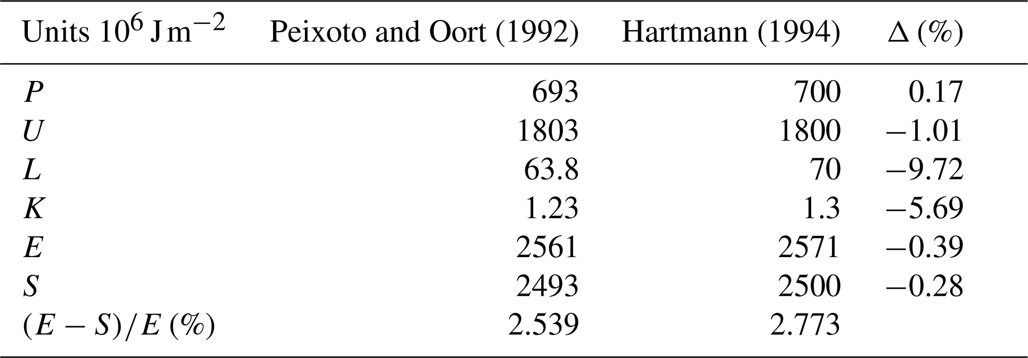

Table 2 Earth's energy comparison.

The sound velocity of an ideal gas is

$$\begin{array}{}\text{(8)}& c=\sqrt{\mathit{\gamma }{\displaystyle \frac{R^{\ast }}{M}}T},\end{array}$$

where R^∗ is the universal constant of gases, and M is the molecular mass of the gas; $\mathit{\gamma }=C_p/C_v$ is the adiabatic constant, and T is the temperature. The sound velocity can be used to estimate the ratio between K and S.

$$\begin{array}{}\text{(9)}& {\displaystyle \frac{K}{S}}\approx {\left({\displaystyle \frac{v}{c}}\right)}^{\mathrm{2}}\end{array}$$

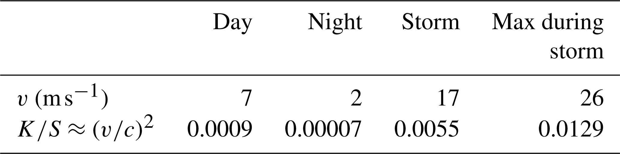
In the case of Mars, on the surface c = 228.73 m s⁻¹. Table 3 contains data of winds measured by Viking probes on the surface (Sheehan, 1996, p. 194). With these data, K can be neglected in Mars. In the case of Titan, Mitchell (2011) assumes that the kinetic energy can be neglected. Based on these figures, the kinetic energy can be omitted in a first approximation for Mars and Titan.

Table 3 Wind velocity in Mars.

In the case when S is not much bigger than K+L, our results for τ would be a lower bound. Future observations will determine these numbers.

3 Absorbed and emitted energy fluxes and residence time in planetary atmospheres

The values of the energy fluxes for all planets have been deduced from Read et al. (2016). For each planet, F_i and F_o represent the inflow and outflow of energy absorbed or emitted by the atmospheres. The so-called “Trenberth diagrams” (Kiehl and Trenberth, 1997; Read et al., 2016) are particularly suited to the identification of these fluxes.

As an example, in the case of Venus (see Read et al., 2016, Fig. 6), the fluxes absorbed by the atmosphere (F_i) are 135 W m⁻² from incoming solar radiation (shortwave) absorbed in the middle atmosphere, 3 W m⁻² from incoming solar radiation absorbed by the lower atmosphere and 17 154 W m⁻² of longwave flux absorbed from surface. Thus, the total influx is 17 292 W m⁻².

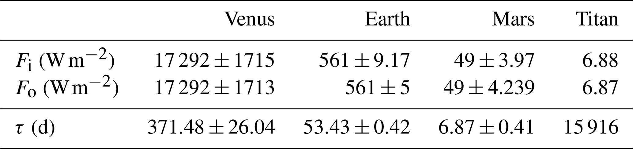
The emitted fluxes (F_o) are 17 132 W m⁻² of longwave radiation to surface and 160 W m⁻² of longwave radiation emitted from atmosphere to space. The total outflux value is 17 292 W m⁻². Analogous calculations for the rest of the planets give the values for F_i and F_o shown in Table 4.

Table 4 Fluxes of energy and residence times in planetary atmospheres.

These energy fluxes were computed by Read et al. (2016) through complex and detailed numerical models. Their results coincide well with observations and have little uncertainty, so its effect on the residence time of energy is small. In any case, here we have computed that uncertainty value.

For Earth, quoting Read et al. (2016, p. 704), “Figure 1 thus represents the current state of the art in deriving such an energy budget for an entire planet.” Although Read et al. (2016) do not give exact numbers for uncertainty of energy fluxes, their references herein do. We have computed the following uncertainty values: F_in = 561 ± 9.17 W m⁻² ⇒ τ = 53.43 ± 0.87 d, and F_out = 561 ± 5 W m⁻² ⇒ τ = 53.43 ± 0.48 d. We note how both fluxes and residence times are extremely similar and compatible. A weighted average would give us τ = 53.43 ± 0.42 d.

When computing the energy fluxes of Mars, Read et al. (2016) use a detailed radiative transfer model “suggesting an uncertainty in infrared fluxes of around 6 %–12 %”. By using the worst-case scenario of a 12 % uncertainty, we obtain F_in = 49 ± 3.97 W m⁻² ⇒ τ = 6.87 ± 0.56 d, and F_out = 49 ± 4.23 W m⁻² ⇒ τ = 53.43 ± 0.59 d. This gives us τ = 6.87 ± 0.41 d. These uncertainties are reflected in Table 4.

About the energy fluxes in Venus, Read et al. (2016) state, “energy fluxes agree with available observations to around ± 10 %”. However, they admit that “the energy budget presented … should therefore be seen as a plausible scheme that is internally self-consistent and representative of a reasonably good radiative–dynamical model of the Venus atmosphere in equilibrium”. Assuming an uncertainty of 10 % in energy fluxes, F_in = 17 292 ± 1715 W m⁻² ⇒ τ = 371.48 ± 36.84 d, and F_out = 17 292 ± 1713 W m⁻² ⇒ τ = 371.48 ± 36.80 d. This gives τ = 371.48 ± 26.04 d.

In Titan's energy fluxes, Read et al. (2016) do not state any bound on uncertainties. However, they say (Read et al., 2016, p. 711) “energy fluxes are consistent with the measurements of Li et al. (2011) to within a few per cent, although the internal and surface fluxes are not well constrained by observations.” We can assume that the energy fluxes they present and used here are fairly accurate with low uncertainty.

With the total energy values, E or S (in Table 1) and F (Table 4), we estimate the value of residence time of energy in the atmosphere of each planet. However, as we stressed above, strictly speaking E is only known in the Earth's case. In the other three cases, the ratio $(S/F)$ is a lower bound for the actual residence time.

$$\begin{array}{}\text{(10)}& {\displaystyle \frac{S}{F}}\le {\displaystyle \frac{E}{F}}=\mathit{\tau }.\end{array}$$

These results and their estimated uncertainties are shown in Table 4.

4 Residence time of energy in the Sun

Although the physics in the solar interior greatly differs from that of a planetary atmosphere, we have considered it convenient to introduce this section because of the parallelism that exists between the atmospheric τ and the solar Kelvin–Helmoholtz timescale.

$$\begin{array}{}\text{(11)}& {\mathit{\tau }}_{\text{KH}}={\displaystyle \frac{G{M}_{\odot }^{\mathrm{2}}}{R_{\odot }{L}_{\odot }}}\sim {\mathrm{10}}^{\mathrm{7}}\mathrm{year},\end{array}$$

where G is the gravitational constant, and M_⊙, R_⊙ and L_⊙ stand for the solar mass, radius and radiant flux.

The Sun is in a steady state for the energy. The temperatures in its interior are not systematically increasing or decreasing. In Stix (2003) it is shown that the Kelvin–Helmholtz timescale (KH) corresponds to both the time that a photon takes from the core until it leaves the surface and the time necessary for the star to return to equilibrium after a global perturbation.

As τ_KH is the ratio between stored energy and its flux, it also can be considered a residence time of energy in the Sun (for details, see Osácar et al., 2020). Furthermore, Spruit (2000) shows that KH is the longest timescale for any solar perturbations.

In summary, if the analogy between the solar KH and the atmospheric τ is assumed, then τ is not only the timescale for the energy transport in the atmosphere but also the timescale the atmosphere needs to return to equilibrium after a global thermal perturbation. Furthermore, τ is the longest timescale for any atmospheric perturbation.

Table 5 Radiative relaxation timescale (τ_r).

5 Discussion

As we concluded in Sect. 4, τ may not only be the mean time it takes for the energy to enter and leave the atmosphere; it may also be the time needed to return to equilibrium after a global thermal perturbation. Although this is likely the case, it does not constitute a proof. But, if this analogy is accepted, it imposes the condition that τ has to be greater than any other relaxation timescale.

In this section, we will introduce the so-called radiative relaxation time, τ_R, and we will explore if the inequality τ>τ_R holds.

In general, if an atmospheric state at equilibrium is perturbed, the atmosphere uses the most efficient mechanism at hand to neutralize it. Typically, this mechanism can be convective, advective or radiative. The radiative relaxation timescale, τ_R, is the time it would take to relax the perturbation by radiating the energy excess in the infrared. This timescale is often found in the literature (e.g. Houghton, 2002; Wells, 2012; Sánchez-Lavega, 2011).

The computation of this timescale τ_R is done by a perturbative method (see, for example, Wells, 2012) and gives

$$\begin{array}{}\text{(12)}& {\mathit{\tau }}_{\mathrm{R}}={\displaystyle \frac{c_{p}p/g}{\mathrm{4}\mathit{\sigma }{T}_{\text{eff}}^{\mathrm{3}}}}.\end{array}$$

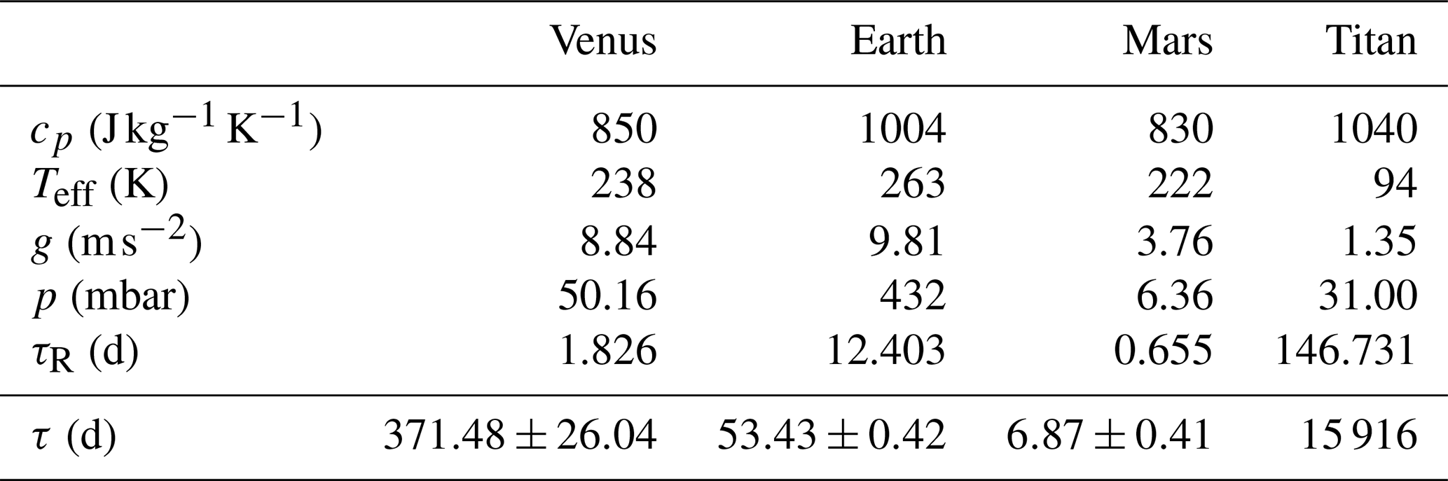
In this expression, c_p is the specific heat at constant pressure, g is gravity and σ is the Stefan–Boltzmann constant. T_eff is the blackbody effective temperature of the planet, and p is the pressure at the height where the computation is performed.

Due to the factor p in the numerator of Eq. (12), the value of τ_R decreases rapidly with height. Therefore, radiation is not an efficient mechanism to neutralize perturbations in the low troposphere. In that region, τ_R is thus very long. The low troposphere is dominated by convective movements. We find a clear example of these phenomena in Venus, where τ_R varies from 116 d at 40 km (lower cloud deck) to 0.5 h at 100 km (Sánchez-Lavega et al., 2017).

Since about 80 % of radiative flux leaving an atmosphere comes from the cold top of the highest atmospheric opaque layer, we have estimated τ_R at the height of maximum emission, p=p_r, which is the pressure at the height where T=T_eff.

In Table 5 we show the results for τ_R in the case of Venus, Earth, Mars and Titan, as well as the data used for calculating them. The data for this table were obtained from Sánchez-Lavega (2011). The values for energy residence time τ are those from the last row of Table 4. In the four cases, the radiative timescale τ_R is shorter than the time of energy residence τ.

If, in any of the planets, the quoted values of τ were a lower bound, as commented in Sect. 2, then the inequality τ>τ_R would be strengthened.