The effect of strong shear on internal solitary-like waves

Large-amplitude internal waves in the ocean propagate in a dynamic, highly variable environment with changes in background current, local depth, and stratification. The Dubreil–Jacotin–Long, or DJL, theory of exact internal solitary waves can account for a background shear, doing so at the cost of algebraic complexity and a lack of a mathematical proof of algorithm convergence. Waves in the presence of shear that is strong enough to preclude theoretical calculations have been reported in observations. We report on high-resolution simulations of stratified adjustment in the presence of strong shear currents. We find instances of large-amplitude solitary-like waves with recirculating cores in parameter regimes for which DJL theory fails and of wave types that are completely different in shape from classical internal solitary waves. Both are spontaneously generated from general initial conditions. Some of the waves observed are associated with critical layers, but others exhibit a propagation speed that is very near the background current maximum. As such they are not freely propagating solitary waves, and a DJL theory would not apply. We thus provide a partial reconciliation between observations and theory.

1 Introduction

Large-amplitude internal waves, often referred to as internal solitary-like waves or ISWs, are a well-studied coherent, nonlinear phenomenon accessible via field measurements, laboratory experiments, and simulations of density stratified fluids. Historically, ISWs were described by approximate perturbation theories that lead to an equation of Korteweg–de Vries (KdV) type for the temporal–horizontal portion of the object (Talipova et al., 1999; Helfrich and Melville, 2006). The vertical component is described by solving a linear ordinary differential eigenvalue problem. This is generally referred to as the weakly nonlinear description, or WNL. While aspects of WNL continue to be actively developed in the recent literature (e.g. Grimshaw et al., 1997; Talipova et al., 1999; Caillol and Grimshaw, 2012), with an excellent survey available in Ostrovsky and Stepanyants (2015), it has been known for some time that WNL is lacking as a quantitative descriptor of ISWs. The KdV theory itself predicts that wave amplitude is bounded above by the onset of breaking, in contrast to observations of wave broadening and the formation of waves with flat crests (i.e. tabletop waves; Lamb and Wan, 1998; Rusås and Grue, 2002). Exact ISWs are solutions of the nonlinear elliptic eigenvalue problem referred to as the Dubreil–Jacotin–Long (DJL) equation. This equation is formally equivalent to the full stratified Euler equations (in a frame moving with the wave), and thus this theory is referred to as fully nonlinear or exact.

Comparisons of WNL with exact ISWs (Lamb and Yan, 1996; Lamb, 1998; Stastna and Peltier, 2005) typically yield poor results for the vertical structure, especially for complex stratifications. Higher-order WNL theory, with the Gardner or mKdV equations as prominent examples, does a better job of qualitatively matching the type of upper bound on wave amplitude (Grimshaw et al., 1997), but there is a significant gap between what is observed in simulations and what WNL can describe (Stastna and Peltier, 2005). In the context of ISWs with strong shear, this gap is well illustrated by the study of Caillol and Grimshaw (2012), which develops a WNL theory for weakly stratified critical layers. The theory is algebraically quite complex, with significant ties to work on Rossby wave critical layers. However, the theory is not compared to simulations or experiments, and thus it is unclear to what extent it applies to a situation with a dynamically evolving wave field. Interestingly, it is very similar in style to Maslowe and Redekopp (1980), which considered a closely linked topic some 30 years earlier.

While field measurements are often taken in a dynamic, complex environment with changes in the stratification structure and a non-trivial background current, much of the understanding of ISWs has been developed based on relatively simple stratifications (typically quasi-two-layer or exponential stratification). The presence of a background shear current complicates the algebra needed to derive theory, whether WNL or the DJL equation. In the case of WNL, the numerical methods are unchanged, but for the DJL equation the iterative algorithm used to obtain solutions requires an ad hoc modification (see Stastna and Lamb, 2002, and the Methods section below). In practice, publicly available software for the DJL equation (Dunphy et al., 2011) can handle many situations, but there is no a priori proof of convergence. It has been shown that the presence of a background shear current can modify the type of upper bound on wave amplitude and can also change the polarity of exact ISWs (again see Stastna and Lamb, 2002, for details). The detail-oriented reader is cautioned that Fig. 3 in Stastna and Lamb (2002) is based on ISWs of elevation which have an opposite sign of wave-induced vorticity to ISWs of depression. For ISWs of depression a background current with positive vorticity tends to decrease the limiting wave amplitude. In his study of ISW energetics in the presence of a background shear current, Lamb (2010) thus employed a negative background current.

The DJL equation has also been extended to model ISWs past breaking or waves with trapped cores. Such waves are known to form during shoaling (Lamb, 2002), and the questions of whether the core is completely trapped (Xu et al., 2016), quiescent (Derzho and Grimshaw, 1997; Lamb and Wilkie, 2004; Luzzatto-Fegiz and Helfrich, 2014), or found to be immediately adjacent to the boundary or at depth (He et al., 2019) have all been the subject of recent studies. Any ISW can be described as a propagating baroclinic vortex, but trapped cores provide a more complex wave–vortex coupling that will be revisited below.

In the classical theory of hydrodynamic stability the gradient Richardson number (Ri) is the standard necessary condition; when Ri>0.25 the flow is linearly stable. However, Ri<0.25 is not a sufficient condition for instability (Hazel, 1972). Large-amplitude ISWs, both with and without a background shear current, can induce strong shear currents near the wave crest. This situation has drawn interest over several decades (Bogucki and Garrett, 1993; Barad and Fringer, 2010; Lamb and Farmer, 2011; Xu et al., 2019), first as a pure conjecture and then with two-dimensional and finally three-dimensional situations. It has been found that shear instability within ISWs is quite complex, with onset dependent on the strength of upstream perturbations, the Reynolds number, and duration of time spent below Ri=0.25 as a perturbation passes through the wave. Three-dimensionalization, at least on scales for which direct numerical simulation (DNS) has been accessible, occurs preferentially at the rear of the wave, and in some parameter regimes instability is episodic, with bursts and quiescent periods.

Walter et al. (2016) measured large-amplitude ISWs in northern Monterey Bay, California (USA), as part of a complex interplay between a coastal upwelling front and local wind forcing. These waves were large amplitude (up to a 10 m maximum isopycnal displacement in water approximately 20 m deep) with strong background shear currents. Indeed, the background shear currents were so strong that solutions of the DJL equation were impossible to compute. Some analysis of large ISW-like waves in the presence of strong background shear currents is provided in Stastna and Walter (2014). These authors considered the resonant generation of ISWs by flow of a background current with shear over isolated topography. They found large-amplitude wave trains as well as waves trapped behind the topography with vortex-rich cores that were quasi-trapped near the surface (i.e. both the upstream-propagating wave trains and the trapped waves exhibited vortex-rich cores). However, the connection between simulations and field measurements is incomplete since it is unclear whether the waves observed in Walter et al. (2016) were resonantly generated.

In recent work, Zhang et al. (2018) considered the effect of a background current on mode-2 waves. The waves were generated via stratified adjustment, similar to the methodology we follow below. The stratification used was centred at the mid-depth, so that in the absence of a shear current initial perturbations have the dominant part of their energy deposited into the mode-2 wave field. The authors document the manner in which the adjustment process and the resulting leading mode-2 wave and trailing mode-1 tail are modified by the presence of shear. They also compare their results to the observations of Shroyer et al. (2010), though the fact that both the density profile and shear layer in Zhang et al. (2018) are centred at the mid-depth makes a detailed comparison impossible.

The interaction of ISWs with background currents has also been explicitly demonstrated in the context of frontal generation. Bourgault et al. (2016) discussed observations and simulations of a case in the Saguenay fjord, Quebec, Canada. The authors found that convergence near the front was important in numerical generation experiments, though the parameter space they explored was fairly limited. In all cases discussed by the authors, rightward- and leftward-propagating wave trains propagating away from the front differ in amplitude, with larger waves observed in stronger shear.

In a related non-ISW context, Lamb and Dunphy (2018) considered the generation of internal waves by tidal flow in the presence of shear. They concentrated on characterizing energy flux and found profound asymmetries between the waves propagating with the shear and against the shear. Interestingly, whether the downstream or upstream side of the ridge that generated the internal waves dominated the energy flux was found to depend on the slope of the flanks of the ridge. It is difficult to ascertain implications of this study for the problem of ISWs with shear, since these authors only considered a linear stratification. Nevertheless, the study clearly suggests that shear can profoundly influence wave energetics.

In this paper, we report on high-resolution simulations of stratified adjustment and the resulting internal wave field in the presence of strong shear currents. The structure of the paper is organized as follows. The Methods section presents the governing equations, the DJL theory, and the design of and parameter values for all numerical experiments we present. The Results section presents the major findings, divided into three parts: (i) waves modified by shear but without critical layers, (ii) waves with critical layers, and (iii) situations in which the stratification is in the opposite half of the water column from the shear layer. The paper concludes with a Discussion section and a brief set of Conclusions.

2 Methods

We consider an incompressible fluid in the absence of rotation that obeys the Boussinesq and rigid lid approximations. The stratified Navier–Stokes equations in the absence of rotation read

$$\begin{array}{}\text{(1)}& {\displaystyle \frac{\partial \mathit{u}}{\partial t}}+\mathit{u}\cdot \mathbf{\nabla }\mathit{u}& {\displaystyle }=-{\displaystyle \frac{\mathrm{1}}{{\mathit{\rho }}_{\mathrm{0}}}}\mathbf{\nabla }P+\mathit{\nu }{\mathrm{\nabla }}^{\mathrm{2}}\mathit{u}-{\displaystyle \frac{\mathit{\rho }g}{{\mathit{\rho }}_{\mathrm{0}}}}\widehat{k},\text{(2)}& {\displaystyle }\mathbf{\nabla }\cdot \mathit{u}& {\displaystyle }=\mathrm{0},\text{(3)}& {\displaystyle \frac{\partial \mathit{\rho }}{\partial t}}+\mathit{u}\cdot \mathbf{\nabla }\mathit{\rho }& {\displaystyle }=\mathit{\kappa }{\mathrm{\nabla }}^{\mathrm{2}}\mathit{\rho },\end{array}$$

where u is the velocity, P is the pressure, ρ is the density, and ρ₀ is some reference density of the fluid. The physical parameters are the molecular kinematic viscosity ν (set to equal $\mathrm{1}\times {\mathrm{10}}^{-\mathrm{6}}$ m s⁻²) and scalar diffusivity κ (set to equal $\mathrm{2}\times {\mathrm{10}}^{-\mathrm{7}}$ m s⁻²). The unit vector in the vertical direction is denoted by $\widehat{k}$. The computational domain is rectangular, with the x axis running left to right along the bottom of the domain, so that $\mathrm{0}<x<L_x$ and $\mathrm{0}<z<L_z$.

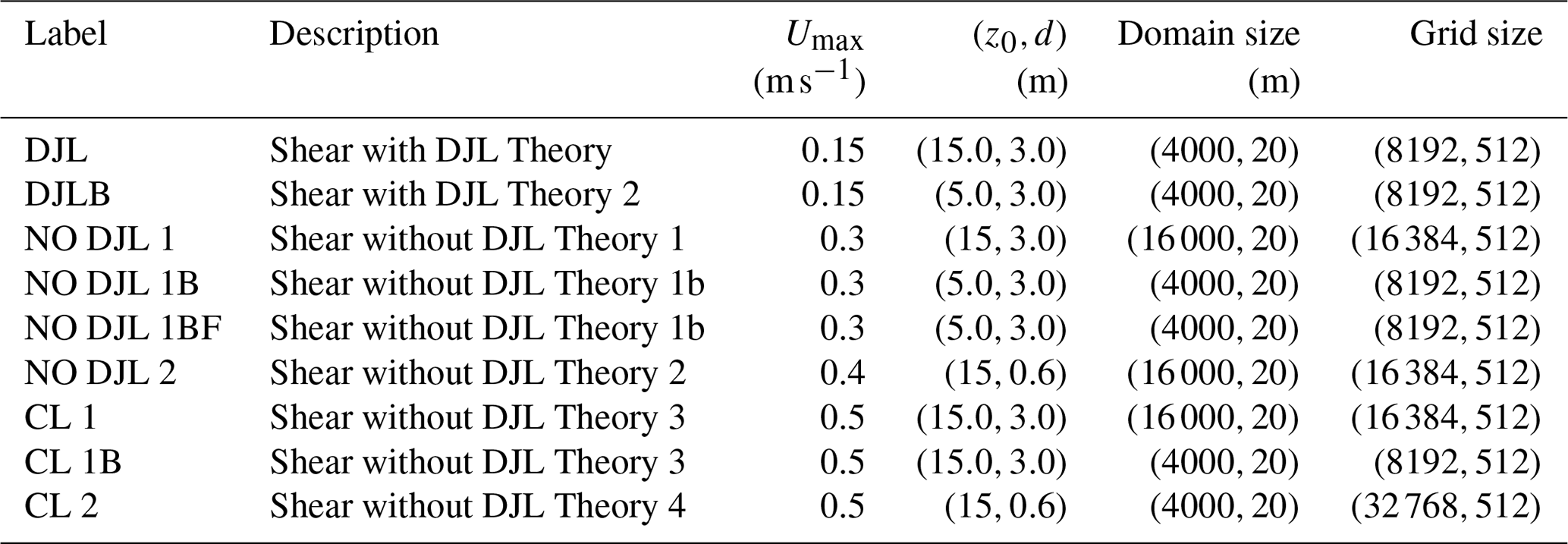
Simulations were carried out with the pseudospectral code SPINS (Subich et al., 2013). The code has been thoroughly validated in a number of different configurations (e.g. shear instabilities, internal wave generation, internal solitary wave propagation) and is available for download through its online manual: https://wiki.math.uwaterloo.ca/fluidswiki/index.php?title=SPINS_User_Guide (last access: 28 September 2021). All simulations reported employed regularly spaced grids. Approximately 30 exploratory simulations were carried out prior to identifying a parameter space of interest. Table 1 provides a list of cases discussed in this paper along with their key physical and numerical parameters. As a general comment, simulations were much higher resolution than many comparable studies in the literature, and the pseudospectral aspect of SPINS means that the model has very little numerical dissipation. This proved vital for some of the results reported below and is discussed further in the Discussion section.

All simulations were initialized with a background shear current

$$\begin{array}{}\text{(4)}& U\left(z\right)=U_{\text{max}}\exp \left[(z-L_z)/d_U\right].\end{array}$$

The total depth was fixed as L_z=20 m for all simulations, but the horizontal extent of simulations was varied on a case-by-case basis. The thickness of the shear layer was fixed at d_U=3 m or 0.15 of the total depth. U_max was varied as described in Table 1. The form of the background current is such that, in the absence of stratification, it is linearly stable (i.e. Fjortoft's criterion is not satisfied).

Table 1 Cases considered throughout the paper, including case label and their dimensional parameters.

The initial density field was specified as $\mathit{\rho }(x,z)=\stackrel{\mathrm{‾}}{\mathit{\rho }}(z-\mathit{\eta })$ with

$$\begin{array}{}\text{(5)}& \mathit{\eta }={\mathit{\eta }}_{\mathrm{0}}\exp \left[-(x-\mathrm{0.5}Lx{)}^{\mathrm{2}}/w_d^{\mathrm{2}}\right].\end{array}$$

While other values were used in preliminary experiments, all numerical experiments reported below set ${\mathit{\eta }}_{\mathrm{0}}=-\mathrm{5}$ m (0.25 of the total depth) and w_d=100 m.

The background density field was specified as

$$\begin{array}{}\text{(6)}& \stackrel{\mathrm{‾}}{\mathit{\rho }}\left(z\right)=\mathrm{1}-{\displaystyle \frac{\mathrm{\Delta }\mathit{\rho }}{\mathrm{2}}}\tanh \left[(z-z_{\mathrm{0}})/d\right].\end{array}$$

The dimensionless density difference was set as Δρ=0.001 for all simulations, while the pycnocline centre and thickness, (z₀,d), were varied as shown in Table 1.

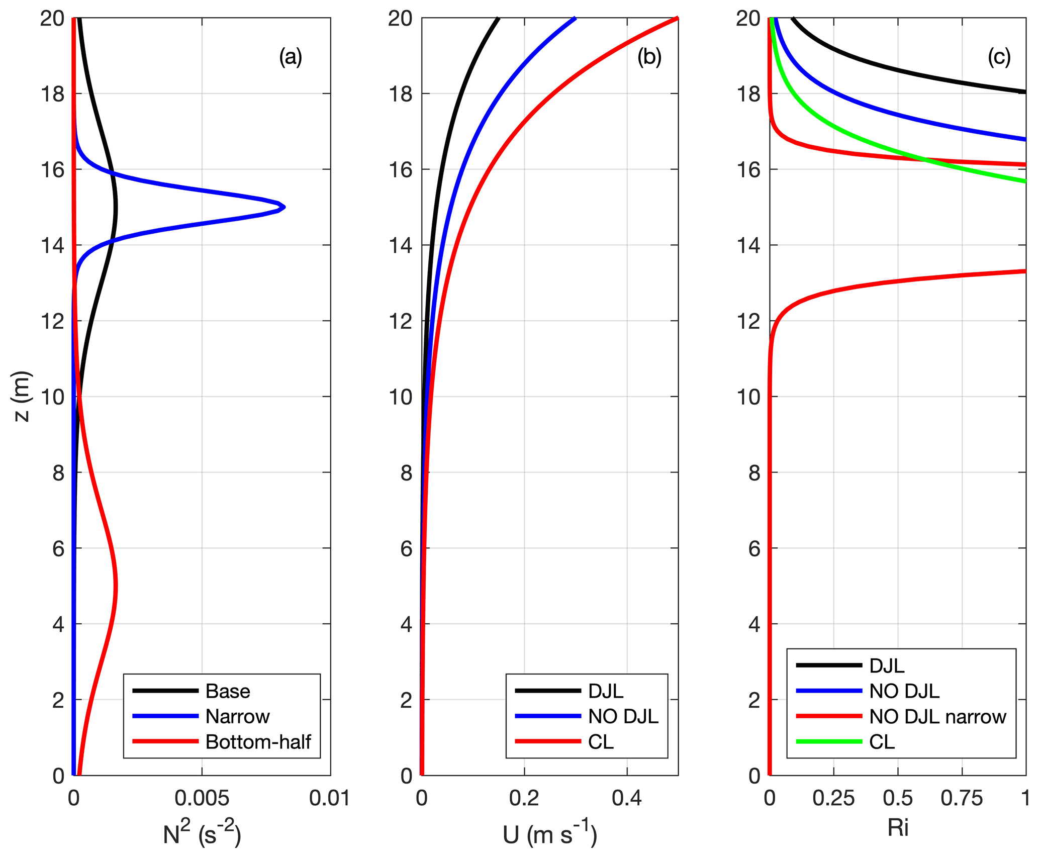
Figure 1 shows a sample representation of the initial conditions, while Fig. 2 shows the 1-D background profiles for the various simulations discussed below. Figure 2a shows the N²(z) profile, Fig. 2b shows the background shear current U(z), and Fig. 2c shows the gradient Richardson number (Ri).

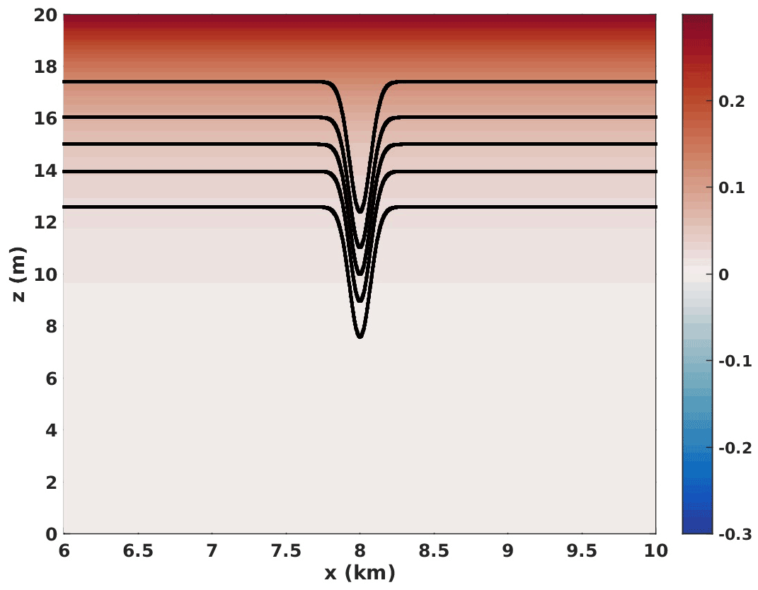
Figure 1 Typical initial conditions. Horizontal component of velocity (m s⁻¹) shaded (case NO DJL 1 shown as a representative sample), five isopycnals in black.

Figure 2 Background profiles. (a) N²(z), (b) U(z), (c) Ri.

Exact internal solitary waves are solutions of the DJL equation. In the presence of a background shear current this equation has a rather complex form:

$$\begin{array}{}\text{(7)}& \begin{array}{rl}{\mathrm{\nabla }}^{\mathrm{2}}\mathit{\eta }& +{\displaystyle \frac{U_z(z-\mathit{\eta })}{\left[U\right(z-\mathit{\eta })-c]}}\left[\mathrm{1}-\left({\mathit{\eta }}_x^{\mathrm{2}}+{\left(\mathrm{1}-{\mathit{\eta }}_z\right)}^{\mathrm{2}}\right)\right]\\ & +{\displaystyle \frac{N^{\mathrm{2}}(z-\mathit{\eta })}{\left[U\right(z-\mathit{\eta })-c{]}^{\mathrm{2}}}}\mathit{\eta }=\mathrm{0}.\end{array}\end{array}$$

For no background current the DJL equation takes the more familiar form

$$\begin{array}{}\text{(8)}& {\mathrm{\nabla }}^{\mathrm{2}}\mathit{\eta }+{\displaystyle \frac{N^{\mathrm{2}}(z-\mathit{\eta })}{c^{\mathrm{2}}}}\mathit{\eta }=\mathrm{0},\end{array}$$

with the strong non-linearity encapsulated in the evaluation of the buoyancy frequency squared profile at its upstream height (i.e. at z−η). While several different techniques for the solution of the DJL equation without a background current are described in the literature, the only publicly available approach to the DJL equation with a background current that the present authors are aware of employs an ad hoc extension of the direct variational method of Turkington et al. (1991), as described in Stastna and Lamb (2002). This consists of an iterative algorithm, which while generally stable for weak currents leads to “wandering” when shear is strong. The simulations reported below specifically concentrate on parameter regimes in which the DJL was found not to converge (unless otherwise noted in the discussion).

2.1 Results

Sample initial conditions are shown in Fig. 1. The horizontal component of velocity is shaded and five isopycnals are superimposed in black. Only a portion of the computational domain is shown. The velocity range is chosen to be symmetric in order to demonstrate that the background current is always greater than or equal to zero. Simulations are reported for combinations of background profiles shown in Fig. 2. In all cases, the region of the highest shear occurs away from the peak in the buoyancy frequency. For cases NO DJL 2 and CL 2 this is due to the thin pycnocline, and for cases with the sub-label B this is due to the fact that the pycnocline centre is below the mid-depth.

Numerical experiments were designed to compare three qualitative categories of results:

1. those with wave trains that have a DJL description propagating both with (rightward) and against (leftward) the background shear current, cases DJL and DJLB;

2. those with wave trains that have a DJL description propagating against the background shear current (leftward) but no DJL description for wave trains propagating with the background shear current (rightward), cases NO DJL 1, NO DJL 1B, NO DJL 1BF, and NO DJL 2; and

3. cases with possible critical layers, cases CL 1, CL 1B, and CL 2.

For cases DJL and DJLB, the background shear current was not large enough to preclude DJL solutions for either the rightward- or leftward-propagating wave trains. Figure 3 shows the leftward- and rightward-propagating wave trains at t=7200 s for cases DJL and DJL B.

Figure 3 Vertical component of the velocity shaded and saturated at ±0.01 m s⁻¹ and eight density contours in black at t=7200 s for cases DJL and DJLB. (a) Case DJL leftward (against shear) propagating wave train and (b) Case DJL rightward (with shear) propagating wave train. (c) Case DJLB leftward (against shear) propagating wave train and (d) Case DJLB rightward (with shear) propagating wave train.

In both cases a rank-ordered wave train is formed, with the leading wave described by solutions of the DJL equation. When the pycnocline is in the upper half of the domain, waves of depression form, and the asymmetry between steeper and taller leftward-propagating (against background shear) waves and broader, shorter rightward-propagating (with background shear) waves is clearly evident. When the pycnocline is in the lower half of the domain, waves of elevation form, the left–right asymmetry is less pronounced, and the fissioning of a rank-ordered wave train takes place more slowly.

The asymmetry of waves that emerge from the initial conditions is consistent with both the KdV and DJL theories (Stastna and Lamb, 2002). In KdV theory the presence of the background current changes the coefficients of nonlinearity and dispersion, while in DJL theory the properties of the solitary waves (such as half width) can be computed from the solution itself. In principle it would be possible to use the inverse scattering theory for the KdV equation to predict the number of solitary waves that emerge from the initial conditions for the leftward and rightward wave trains, but at the time of writing the authors are unaware of a practical implementation of this technique.

2.2 Solitary-like wave trains without DJL theory

We now turn to the more dynamically interesting cases for which DJL theory proves incomplete. We first consider the case labelled NO DJL 1. The stratification corresponds to the black curve in Fig. 2a, while the background shear current corresponds to the blue curve in Fig. 2b. This case yields coherent wave trains propagating both with and against the background shear current, but the iterative DJL solver is not able to converge to steady solutions for the rightward-propagating waves going with the background shear current. This is almost certainly due to the low values of Ri in the shear layer, as indicated by the blue curve in Fig. 2c.

Figure 4 shows the density field in panel (a) and the vertical component of velocity, or w, in panel (b). The response of the density field at this advanced time (t=21 600 s) is clear: two wave trains form, with propagation distance altered by the Doppler shift due to the vertical mean of the background current. A large-amplitude wave train propagates against the shear current (waves are leftward-propagating). Its constituent waves are rank-ordered with no sign of instability. The portion of the domain between $\mathrm{8}\mathrm{km}<x<\mathrm{12}$ km is dominated by the remnant of the adjustment process or the portion of the initial disturbance that is deformed by the background shear current to form an overturning region. The wave train propagating with the shear current (waves are rightward-propagating) can be seen for x>14 km. Again, the waves appear rank-ordered but are smaller in amplitude and much wider than the waves that make up the leftward-propagating wave train (moving against the shear current).

Figure 4 Sample wave trains at a late time (t=21 600 s) for Case NO DJL 1. (a) Scaled density and (b) vertical component of velocity.

Figure 5 revisits the above comment on stability but at two earlier points in the evolution of the wave trains, namely, at t=3600 and 7200 s. We show Ri using a symmetric colour range, whereby the blue regions denote static instability (N²<0). It can be seen that remnants of the initial adjustment yield a very large region of overturns, as the initial density perturbation is strained by the background current. Interestingly, even at early times, some overturning extends to very near the front of the rightward (or with the background shear current) propagating wave train. The leading rightward-propagating wave is evident at t=3600 s, and at t=7200 s three rank-ordered waves have separated from the region of instability. At 7200 s a Rayleigh–Taylor-type instability is observed at the bottom of the shear layer ($\mathrm{17}<z<\mathrm{19}$ m) for $\mathrm{8.6}<x<\mathrm{9.1}$ km. All three rightward-propagating waves exhibit overturns (blue regions) in their core, while the adjustment remnants yield a region of Ri<0.25 over a region spanning several kilometres near the upper boundary. In contrast, the leftward-propagating (or against the background shear current) wave train only yields regions with Ri<0.25 very near to the upper boundary, with no overturns observed.

Figure 5 Case NO DJL 1. Ri at (a) 3600 s and (b) t=7200 s. Colour range saturated over $-\mathrm{0.25}<\mathit{Ri}<\mathrm{0.25}$.

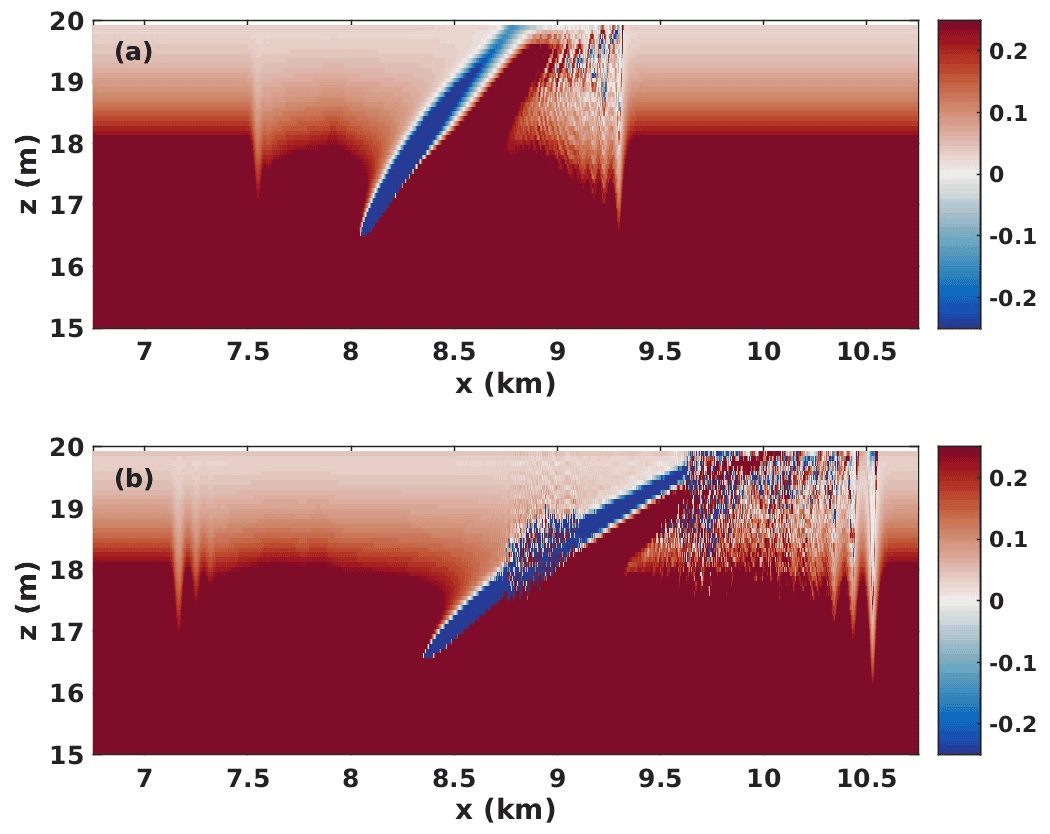
There are thus three different types of instability observed in these cases: (i) Rayleigh–Taylor type instability that occurs beneath the background shear current, (ii) a stratified shear instability triggered by the stratified adjustment of the rightward-propagating wave train, and (iii) the generation of strong vortex cores in the leading ISW-like waves of the rightward-propagating wave train.

The detailed evolution of the wave trains, as expressed in the density field, is shown in Figs. 6 and 7. Three times are shown (t=7200, 14 400, and 21 600 s), with a domain that extends 1 km in the horizontal but shifts locations as the wave train propagates. If the reader was not told of its presence in Fig. 6, they would have no reason to suspect that a background shear current was present, as the leftward-propagating (against the shear) waves take the form of classical “bell-shaped” solitary waves of both WNL and DJL theories. This is in sharp contrast to rightward-propagating (with the shear) waves in Fig. 7. Here the region near the upper boundary is clearly active, with shortwave and “roll” activity evident over a significant portion of the domain. The leading waves take a very different form from classical solitary waves, with sharp crests more akin to Stokes waves or cnoidal waves (Rubenstein, 1999). Figure 8 reconsiders the near upper boundary region (top 2 m of the domain) for the wave train propagating rightward with the shear current. Forty density isolines that range over ${\mathit{\rho }}_{\text{min}}<\mathit{\rho }<{\mathit{\rho }}_{\text{min}}+\mathrm{0.2}\mathrm{\Delta }\mathit{\rho }$ are shown. By concentrating the view on this region, it can be seen just how active the near-boundary region is. Not only do the rightward-propagating waves exhibit quasi-trapped, recirculating cores that remain active over a long time period, but it can also be seen that a tumultuous region of overturns and rolls initially nearly reaches the two leading waves but gradually lags behind. This figure clearly illustrates that the most important feature of internal solitary-like waves is their ability to outrun localized regions of overturns and instability (which we labelled instability ii above) before such regions drain significant energy from the wave. However, because it takes some time for the solitary-like waves to fission, there is ample time to trigger stratified shear instabilities over a wide spatial region.

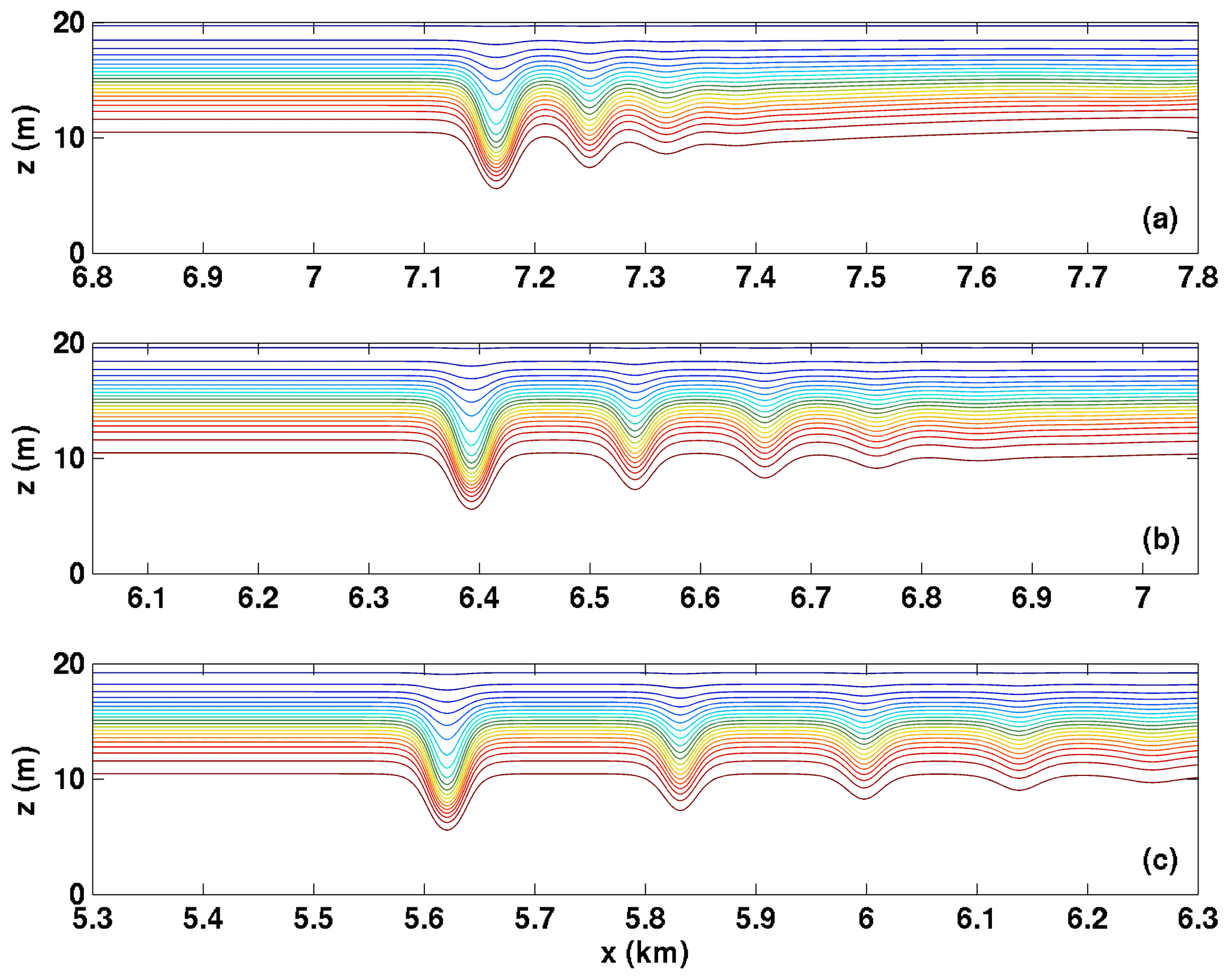
Figure 6 Density fields for wave trains propagating against the shear current for Case NO DJL 1. (a) t=7200 s, (b) t=14 400 s, and (c) t=21 600 s.

Figure 7 Density fields for wave trains propagating with the shear current for Case NO DJL 1. (a) t=7200 s, (b) t=14 400 s, and (c) t=21 600 s.

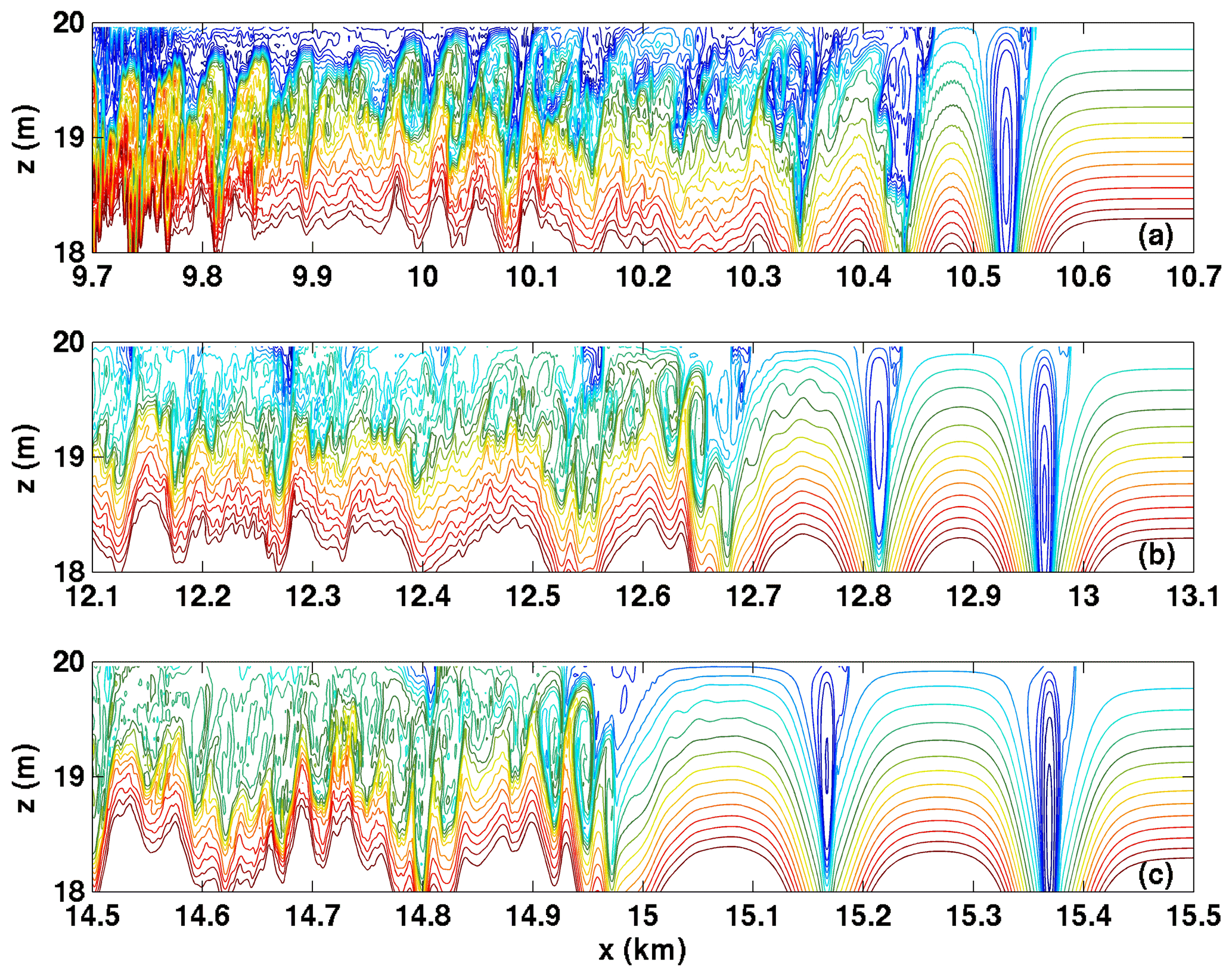
Figure 8 Detail of density fields in the core region for wave trains propagating with the shear current for Case NO DJL 1. Twenty-one density isolines with values $-\mathrm{5}\times {\mathrm{10}}^{-\mathrm{4}}<\mathit{\rho }<-\mathrm{4}\times {\mathrm{10}}^{-\mathrm{4}}$ shown. (a) t=7200 s, (b) t=14 400 s, and (c) t=21 600 s.

In Table 2, we show estimates of the propagation speed of the leading rightward-propagating wave going with the background current. It is immediately evident that all the cases discussed above have propagation speeds (c_est) that are very near the background current maximum (U_max). Moreover, the scaled propagation speed ($c_{\text{est}}/U_{\text{max}}$) tends toward 1 as U_max increases. The DJL theory assumes that streamlines (in a frame moving with the wave) connect to infinity both upstream and downstream of the wave. This is not the case for the NO DJL cases. We hypothesize that this is why the DJL solvers fail to converge in this parameter range. Essentially, the wave trains that form cannot be fully decoupled from the adjustment region for a long enough time so that vortex-dominated leading waves (or several waves) form.

Table 2 Estimated wave speeds for select cases.

To summarize, in all the “NO DJL” cases shown in Table 1, rightward-propagating (with the background shear current) waves with trapped cores and near-surface regions of overturns and local instabilities were consistently observed. These waves cannot be described by presently available solvers for the DJL equation. In all simulations they were observed to be long-lived, with active core regions that could transport mass over a considerable distance in the field.

2.3 Wave trains with critical layers

The waves described in the previous section (all “NO DJL” cases) were found to have propagation speeds that were greater, if only marginally, than the maximum background shear current. When $U_{\text{max}}>c>\mathrm{0}$, a critical layer may form. In order to get some sense of how robust the waves described above are to the presence of a critical layer, we present the results of two cases with U_max=0.5 m s⁻¹. In Fig. 9 we show the vertical velocity and density fields over the top 4 m for the wave train propagating rightward with the background current at three different times. The leading and second waves are shown, with both exhibiting a prominent quasi-trapped, recirculating core. Interestingly, while the quasi-trapped core of the leading wave appears relatively quiescent, a region of instability is observed ahead of it, near the top boundary.

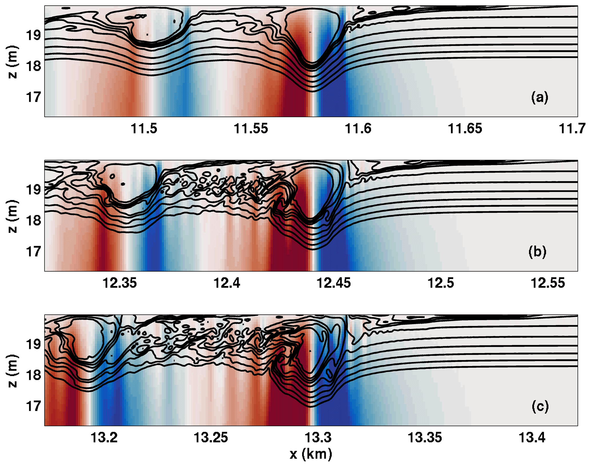
Figure 9 Detail of vertical velocity (shaded and saturated at ±0.01 m s⁻¹) and density fields in the core region for wave trains propagating with the shear current critical layer case CL 1. Ten density isolines with $-\mathrm{5}\times {\mathrm{10}}^{-\mathrm{4}}<\mathit{\rho }<-\mathrm{4}\times {\mathrm{10}}^{-\mathrm{4}}$ shown in black. (a) t=7200 s, (b) t=9000 s, and (c) t=10 800 s.

The majority of the rightward-propagating wave trains described above involved trapped cores. In contrast, the cases with DJL theory yield non-breaking waves. In order to explore the effect of stratification in the high-shear region, we performed a series of experiments with a narrower pycnocline and report one representative example, case CL 2. We found that the leading waves no longer matched the bell-shaped internal solitary waves of DJL theory and that the short length-scale behaviour in the high-shear region required a substantial increase in horizontal resolution (Δx=0.12 m for this case). In Fig. 10a we show the density field for the rightward-propagating wave train. Note that the horizontal length is reported in metres, as opposed to kilometres for the previous figures. The leading wave can be seen to be horizontally asymmetric, with isopycnals in the region downstream of the crest that do not return to their upstream height. Figure 10b and c show the horizontal component of velocity saturated between ±0.005 m s⁻¹. Figure 10b corresponds to the region between thick black lines in panel (a), while panel (c) corresponds to the region between thin dashed black lines in panel (a). Figure 10b and c show only the upper 2 m of the water column. Figure 10c exhibits an inner region of strong vertical currents and a broader region of weaker currents. The outer region extends much further upstream of the wave crest (faint blue) than downstream (faint red). The leading wave is trailed by a long wave train. Figure 10b shows that the vertical currents in the wave train exhibit similar, short length-scale fluctuations near the upper boundary (where the presumed critical layer is located).

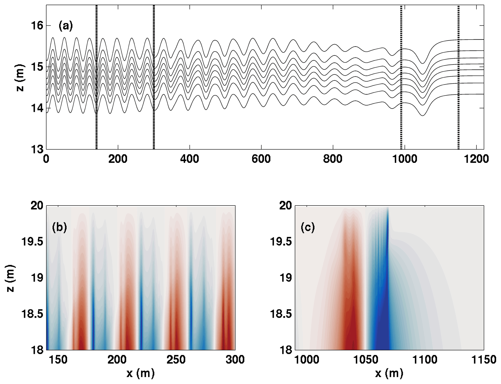
Figure 10 (a) Detail of density fields for wave trains propagating with the shear current critical layer case CL 2 (the case with a narrow density profile) t=4500 s, (b) the vertical velocity component in the top 2 m of the domain in the region between the thick black lines in (a) saturated at ±0.005 m s⁻¹, and (c) the vertical velocity component in the top 2 m of the domain in the region between the thin dotted black lines in (a), saturated at ±0.005 m s⁻¹.

Figure 11 The relative vorticity field saturated at 0.1 s⁻¹ for the CL2 case with the density field overlain at t=4500 s.

The relationship between the rightward-propagating wave train and the background current is better illustrated via the relative vorticity field, ${\mathit{\omega }}_{\text{relative}}=u_z-w_x-U^{\prime }\left(z\right)$, where U(z) is the background shear current. The relative vorticity field is shown in Fig. 11. It can be seen that the leading wave has a substantial vortex that is trapped near the upper boundary. The wave train behind the leading wave is associated with a train of vortices that gradually descends from the upper boundary into the main water column. Thus, what is referred to as “the leading wave” above is, to a substantial degree, a deformation of the pycnocline by the leading vortex.

2.4 Wave trains with unstratified shear layers

The results in Fig. 11 suggest that stratification in the shear layer region has a profound influence on the type of wave that forms via adjustment. In the absence of a shear layer, a pycnocline located in the bottom half of the water column yields ISWs of elevation. We thus performed a number of numerical experiments with a pycnocline located in the bottom half of the water column to see whether wave trains of elevation behave similarly to those reported above.

The results of our numerical experiments indicate that waves propagating against the background current are far less affected when the pycnocline is well removed from the shear layer. In contrast, ISWs propagating with the shear are almost completely destroyed in all but the weakest currents that were tried. Figure 12 shows the vertical component of the velocity field shaded with a saturation with eight density isolines superimposed. The strength of the background shear current increases from top to bottom. In the weakest shear current case (Fig. 12a) the trademark updraft–downdraft pattern of a DJL ISW can be seen for both the rightward- and leftward-propagating wave trains. At the time shown, the wave train has not fully fissioned into rank-ordered ISWs. The reason for selecting such an early time in the evolution, t=5400 s, can be observed in the bottom two panels. Figure. 12b and c show U₀=0.3 m s⁻¹ and U₀=0.5 m s⁻¹, respectively. In both cases there is no trace of a coherent rightward-propagating wave train, and the perturbation vertical velocity field is dominated by relatively short length-scale perturbations. In Fig. 12b an argument could be made for a weak wave train, but unlike Fig. 7 there is no clear separation between a leading wave form and the trailing waves. In the highest velocity case the remnants of the rightward-propagating wave train trail the disturbances near the surface by at least 1000 m.

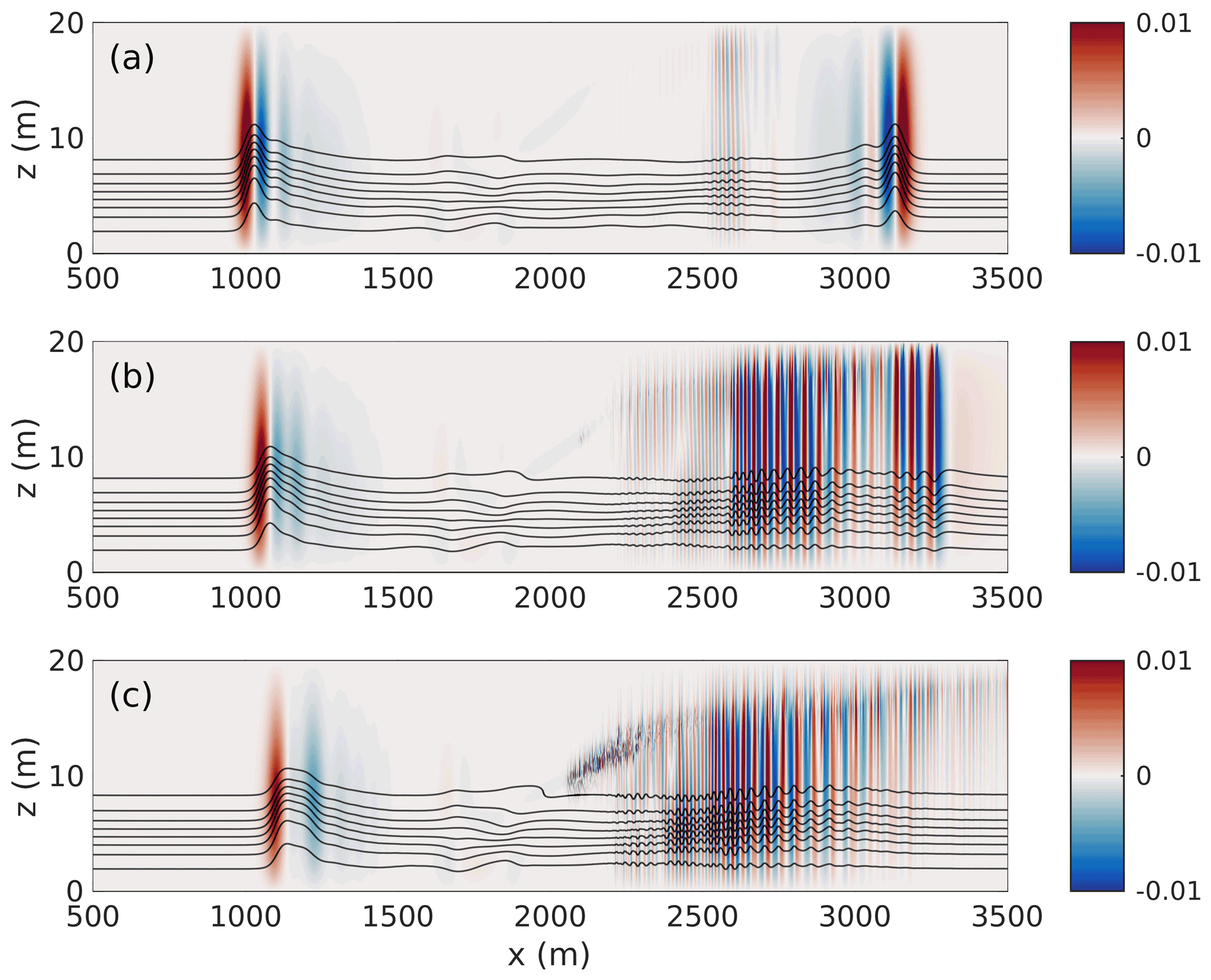
Figure 12 The vertical component of velocity (shaded) saturated at ±0.01 m s⁻¹ with eight isolines of density superimposed at t=5400 s. (a) Case DJLB, (b) case NO DJL 1B, and (c) case CL 1B.

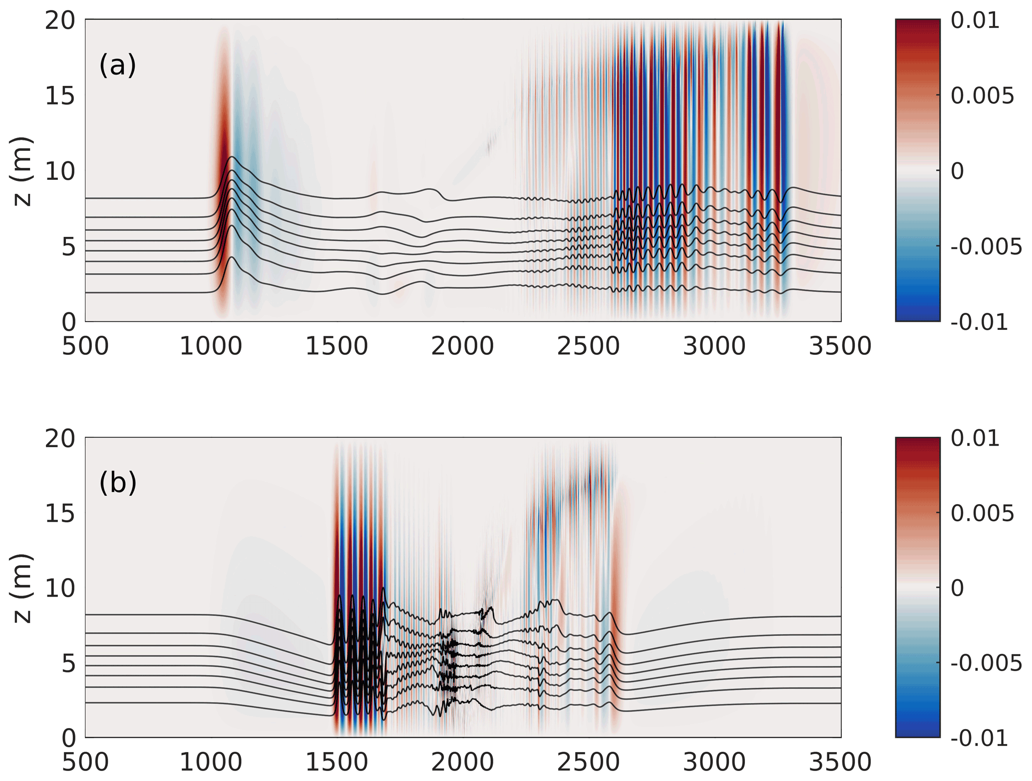
Figure 13 The vertical component of velocity (shaded) saturated at ±0.01 m s⁻¹ with eight isolines of density superimposed at t=5400 s. (a) Case NO DJL 1B and (b) case NO DJL 1BF (polarity reversal).

Since background shear has been found to possibly affect the polarity of ISWs, we performed numerical experiments with an initial condition with reversed polarity (a depression). The results of polarity reversal are compared for U₀=0.3 m s⁻¹ in Fig. 13. Figure 13a reproduces Fig. 12b, while Fig. 13b shows the polarity-reversed case. It can be seen that the leftward-propagating wave in Fig. 13b takes the form of an undular bore, consistent with the predictions of WNL theory. The undular bore is much slower than all ISWs previously simulated. Interestingly, the rightward-propagating wave train also yields an undular bore; however, for later times (not shown) the undular bore largely fades away to irrelevance, and the disturbances of the high-shear region dominate the rightward-propagating response.

The cases described in this subsection are perhaps the clearest demonstration of the difference between the weak-shear regime discussed in Stastna and Lamb (2002) for which ISWs are modulated in form by the background shear current and the strong background shear regime.

3 Discussion

The numerical experiments reported above illustrate that when a strong background shear current is present, the set of possible wave–vortex phenomena is considerably larger than the tidy ISWs described by the DJL equation. Indeed, essentially none of the phenomena we have simulated could be termed truly steady. The main coherent feature from our simulations one could expect to see in the field, for a strong background shear current, are ISWs with a strong vortex core in the near-surface, high-shear region. Classical theory of ISWs with cores generally considers nearly quiescent cores (Derzho and Grimshaw, 1997; Luzzatto-Fegiz and Helfrich, 2014; Lamb and Wilkie, 2004), while recent theory and simulations that include background shear currents yield so-called “subsurface cores” (He et al., 2019). Neither of these matches the strong wave–vortex coupling that was observed above (e.g. Fig. 8). In cases in which a critical layer is possible, the vortex cores coexist with smaller disturbances that extend ahead of the leading ISW.

The simulations we performed required resolution that was much higher than that typically used in coastal ocean simulations (i.e. multi-kilometre domains with a horizontal resolution of less than a metre and a vertical resolution of less than 5 cm). Even recent process studies on mode-2 waves in the presence of shear using the finite-volume MITgcm (Zhang et al., 2018) used a resolution of 5×0.5 m (which was more than sufficient for the phenomena these authors set out to model). Moreover, the pseudospectral model used has very low inherent numerical dissipation, so that even phenomena with relatively few grid points across them are only weakly damped. The high resolution necessarily makes extension to three dimensions a complicated task. However, 3-D simulations initialized from a 2-D simulation, i.e. using the early portion of the simulations described above, should be possible with present computational resources. It is likely that performing a detailed energy analysis, as in Lamb (2010) for ISWs propagating against the background shear current (hence ones with a DJL theory), would require 3-D simulations.

However, a more serious issue when interpreting the above results is in the large gap between theory-inspired simulations and those on the regional scale in coastal oceans. To the authors' knowledge there has been no systematic study of ISW behaviour in marginally resolved situations, especially when parameterizations for mixed layers (e.g. the KPP scheme) are employed. As noted above, the key feature of ISWs is their ability to outrun local instabilities or mixing events without a loss of coherence. A globally high value of eddy viscosity cannot be “outrun”, and thus care should be taken in extrapolating simulation results to particular field measurements.

Even with the above caveats, the simulations we have conducted pose a very clear question for the theorist: “In deep water in which a pycnocline may be far removed from local shear layers can an ISW be destabilized by a shear that would be thought of as so far from the wave that it would be irrelevant to its evolution?”

4 Conclusions

We have provided one possible explanation for why the measurements in Walter et al. (2016) yielded large-amplitude waves with no DJL-based description. That is, that for a portion of parameter space, mode-1 ISWs generated via stratified adjustment in the presence of a background shear current are not free waves, since they have a propagation speed very close to the maximum value of the background current. When some stratification is observed near the surface, these waves take the form of ISWs with strongly recirculating cores.

The simulations above were 2-D, while the observations of Walter et al. (2016) were influenced by rotation and likely included some large-scale 3-D structures (comments on small-scale three-dimensionalization were made in the Discussion above). Moreover, the observations take a different form from the wave trains that are spontaneously generated in our stratified adjustment simulations. This is not surprising, and a set of initial conditions more closely tied to the field observations remains a clear goal for future work.

A different avenue for future work would be to more closely link our results to the work of Zhang et al. (2018) on mode-2 waves. Mode-2 waves lack a DJL theory due to the possible presence of a trailing tail of mode-1 waves, and the question of whether a particular shear current more strongly affects the leading mode-2 wave or its mode-1 tail remains largely open.

Finally, we provided well-resolved examples of stratified adjustment with critical layers (cases labelled “CL”). When a significant stratification was present near the surface, the waves formed consisted of strong vortex cores, with some evidence of fine-scale structure on the leading side of the wave. In the absence of stratification near the surface, a train of vortices spontaneously formed near the surface, and this led to small-amplitude deformations of the underlying pycnocline. Our simulations did not yield evidence of the common theoretical assumption that ISWs are the dominant object, with critical layers providing a slow drain of energy (Caillol and Grimshaw, 2012). This observation should be re-examined on scales for which 3-D DNS is possible.