the Creative Commons Attribution 4.0 License.
the Creative Commons Attribution 4.0 License.
 | 14 Sep 2021
Enhanced diapycnal mixing with polarity-reversing internal solitary waves revealed by seismic reflection data
Yi Gong
Zhongxiang Zhao
Yongxian Guan
Kun Zhang
Yunyan Kuang
Wenhao Fan
Shoaling internal solitary waves near the Dongsha Atoll in the South China Sea dissipate their energy and enhance diapycnal mixing, which have an important impact on the oceanic environment and primary productivity. The enhanced diapycnal mixing is patchy and instantaneous. Evaluating its spatiotemporal distribution requires comprehensive observation data. Fortunately, seismic oceanography meets the requirements, thanks to its high spatial resolution and large spatial coverage. In this paper, we studied three internal solitary waves in reversing polarity near the Dongsha Atoll and calculated their spatial distribution of diapycnal diffusivity. Our results show that the average diffusivities along three survey lines are 2 orders of magnitude larger than the open-ocean value. The average diffusivity in internal solitary waves with reversing polarity is 3 times that of the non-polarity reversal region. The diapycnal diffusivity is higher at the front of one internal solitary wave and gradually decreases from shallow to deep water in the vertical direction. Our results also indicate that (1) the enhanced diapycnal diffusivity is related to reflection seismic events, (2) convective instability and shear instability may both contribute to the enhanced diapycnal mixing in the polarity-reversing process, and (3) the difference between our results and Richardson-number-dependent turbulence parameterizations is about 2–3 orders of magnitude, but its vertical distribution is almost the same.
- Article
(14236 KB) - Full-text XML
- BibTeX
- EndNote


Energy dissipation of internal waves enhances diapycnal mixing. Turbulence in the form of internal wave breaking is the primary mechanism for modifying thermodynamic properties in the ocean (St. Laurent et al., 2011). Small-scale changes in topography also significantly enhance local mixing (Nash and Moum, 2001; Klymak et al., 2008; Palmer et al., 2013; Staalstrøm et al., 2015; Wijesekera et al., 2020; Voet et al., 2020). Internal tides and internal waves are ubiquitous on the global continental shelves and slopes (Holloway, 2001; Sharples et al., 2001; Xu et al., 2010, 2016; Zhang and Alford, 2015; Alford et al., 2015). They play an important role in the global oceanic energy balance and provide energy for ocean mixing (MacKinnon and Gregg, 2003). Due to shoaling internal waves and seafloor roughness, turbulent mixing on the continental shelves and slopes is more variable than in the open ocean (Carter et al., 2005). Diapycnal diffusivity observed on continental shelves and slopes can span 4 orders of magnitude (Gregg and Özsoy, 1999; Nash and Moum, 2001). Internal solitary waves are a kind of nonlinear internal wave, which usually carries a large amount of energy. Numerical simulations indicate that up to 73 % of the internal wave energy can be carried by internal solitary waves (Bogucki et al., 1997). Therefore, internal solitary waves propagating to the continental shelf and slope can greatly change the local mixing. A number of studies have been carried out on mixing caused by internal solitary waves on the continental shelf and slope. Observations have shown that turbulence induced by shear instability at the rear of internal solitary waves sharply increases mixing (Sandstrom et al., 1989; Sandstrom and Oakey, 1995; Moum et al., 2003; Richards et al., 2013). MacKinnon and Gregg (2003) estimated that 50 % of the dissipation in the thermocline occurred with internal solitary waves. In particular, elevation internal solitary waves propagating near the seafloor enhance mixing, resuspending and transporting materials, which has an important impact on the local ecological environment (Klymak and Moum, 2003; Moum et al., 2007b).
Internal solitary waves are ubiquitous in the northeastern South China Sea (Zhao, 2003; Klymak et al., 2006; Xu et al., 2010; Cai et al., 2012; Alford et al., 2015). They are mainly generated either by nonlinear steepening of internal tides from the Luzon Strait or on local continental slopes (Alford et al., 2015; Xu et al., 2016; Min et al., 2019). Some internal solitary waves propagate toward the Dongsha Atoll, where their energy is dissipated in shoaling. The continental shelf and slope of the northeastern South China Sea are close to the source, so that the amplitude and energy of internal solitary waves in this area are large. The energy dissipation of internal solitary waves occurs most near the Dongsha Atoll and its southeastern shelf (Lien et al., 2005; Chang et al., 2006; St. Laurent, 2008). Observations show that high turbulence mainly occurs in the continental shelf region, and the average diffusivity can reach O(10−3) m2 s−1, while the diffusivity in the continental slope region is 1 order of magnitude lower (Yang et al., 2014). When nonlinear internal waves travel cross the continental slope, their waveform changes into different types (Terletska et al., 2020). In this process, mixing is enhanced, and about 30 % of the energy dissipation occurs near the seafloor (St. Laurent, 2008). The energy flux of internal solitary waves around the Dongsha Plateau is large. Lien et al. (2005) estimated that, if all nonlinear internal waves break within a water depth of 10 m and in an area of 200 × 200 km2 centered on the Dongsha Plateau, the magnitude of diffusivity can exceed O(10−3) m2 s−1. In addition, internal solitary waves shoaling near the Dongsha Atoll also dissipate a lot of energy and improve the local mixing efficiency (Orr and Mignerey, 2003; St. Laurent et al., 2011). The water in the northeastern South China Sea can exchange heat with the water in the Pacific Ocean through the Kuroshio (Jan et al., 2012; Park and Farmer, 2013; Xu et al., 2021), and heat can be transferred to the atmosphere through the sea–air interface on the continental shelf. Therefore, internal solitary waves are an important link for energy transfer in the South China Sea and play an important role in our understanding of energy transfer between the ocean and climate environment.
Turbulence in the ocean is patchy and instantaneous. Therefore, it requires extensive observations to accurately evaluate turbulent mixing (Whalen et al., 2012; Waterhouse et al., 2014; Kunze, 2017). Seismic oceanography (Holbrook et al., 2003) has the advantages of wide observation range and high spatial resolution (Ruddick et al., 2009), which are suitable for observing the spatial distribution of turbulent mixing. Sheen et al. (2009) used reflection seismic data to give a diffusivity section of the oceanic front in the South Atlantic. Holbrook et al. (2013) comprehensively introduced the theoretical basis for evaluating turbulent mixing from reflection seismic data. Subsequently, a large number of scholars have used the reflection seismic method to study the spatial distribution of turbulent mixing in different ocean regions or turbulent mixing induced by different ocean phenomena (Fortin et al., 2016; Sallarès et al., 2016; Dickinson et al., 2017; Mojica et al., 2018).
In this article, we used two-dimensional seismic data to observe the propagation of internal solitary waves near the Dongsha Atoll and calculated the spatial distribution of local diapycnal diffusivity to evaluate the impact of internal solitary waves shoaling on turbulent mixing. Section 2 introduces seismic data processing and the method of calculating turbulence mixing parameters. Section 3 describes the polarity reversal of internal solitary waves, the horizontal slope spectrum and the distribution of turbulence diffusivity. In Sect. 4 we analyze the relationship between diapycnal diffusivity and reflection seismic events and discuss the mechanism of turbulent mixing induced by internal solitary waves. In addition, we compare the mixing scheme with our results. Section 5 gives a summary.
2.1 Seismic data acquisition and processing
The water is shallow on the continental shelf and slope near the Dongsha Atoll, so internal solitary waves reach the transition point and their polarity changes from depression to elevation. In the summer of 2009, the Guangzhou Marine Geological Survey (GMGS) set up a two-dimensional seismic observation network in the Dongsha area. We found three internal solitary waves during the polarity reversal process on the L1, L2, and L3 survey lines of the seismic data. The survey lines are shown in Fig. 1a, b. The streamer used in the acquisition process has a total length of 6 km and 480 channels, the trace interval is 12.5 m, and the sampling interval is 2 ms. The airgun source capacity is 5080 in.3 (1 in. = 2.54 cm), and the main frequency of the source is 35 Hz. The shot interval is 25 m, and the minimum offset is 250 m. The time interval of shots is about 10 s. Survey lines L1 and L2 are the in-lines, which were from the southeast to the northwest. Survey line L3 is a cross-line, which was from southwest to northeast. We calculated the mean buoyancy frequency (Fig. 1c) of the region around seismic survey lines (latitude range 21.5–22.5∘, longitude range 116–118∘, blue box in Fig. 1a) by reanalysis temperature and salinity data with a water depth of 100–350 m. This depth range matches the observation depth of the seismic data. Besides, since the buoyancy frequency changes seasonally, we only selected the buoyancy frequency from July to August in 2009, which matches the seismic data observation time. The hydrographic data are provided by the Copernicus Marine Environment Monitoring Service (CMEMS).
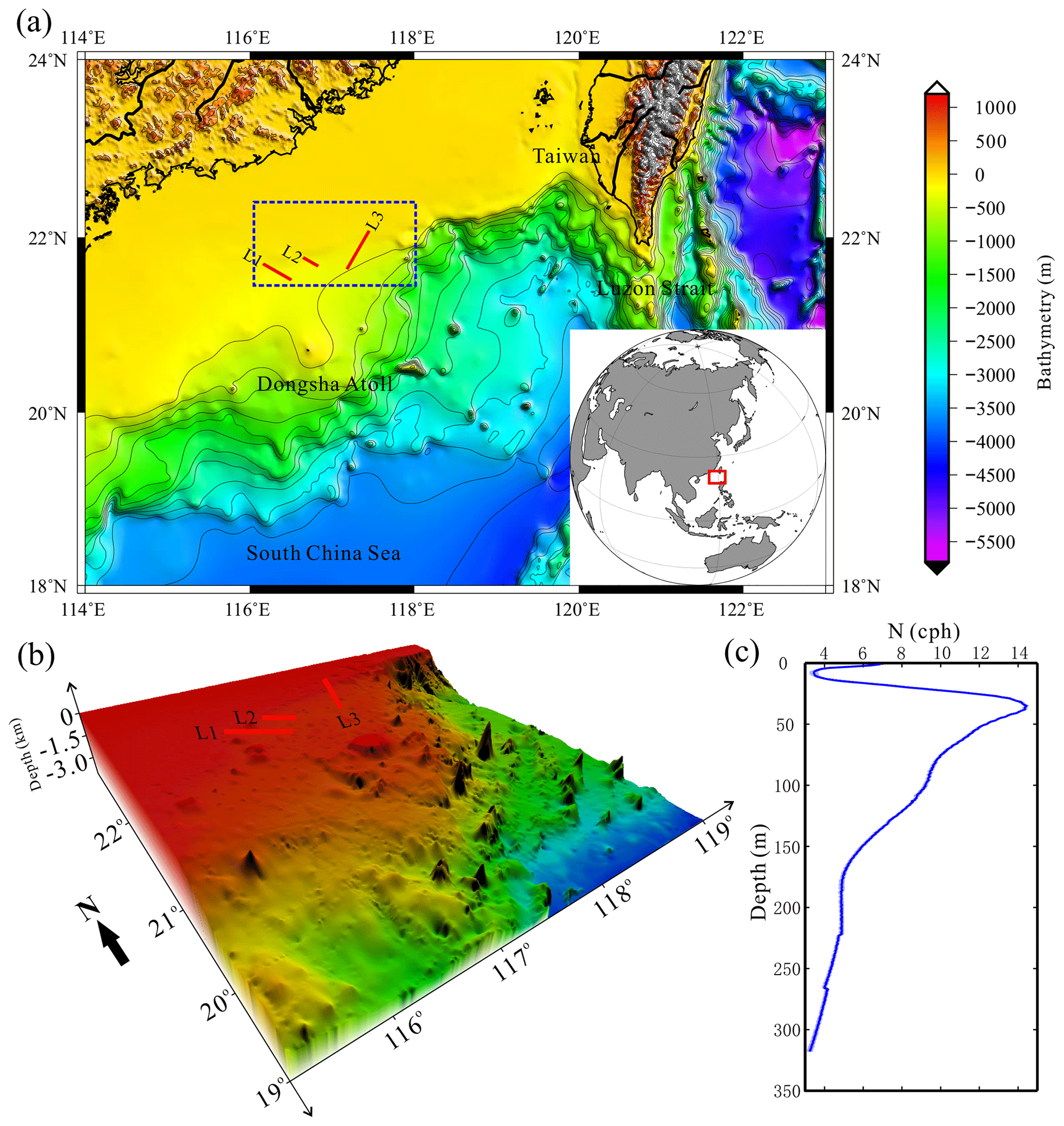
Figure 1Bathymetry of the Dongsha area and locations of seismic survey lines. (a) Two-dimensional bathymetric map of the northeastern South China Sea, with the red lines representing the seismic survey lines. (b) Three-dimensional bathymetric map around the Dongsha Atoll. (c) The mean buoyancy frequency (cph: cycles per hour) around seismic survey lines (blue box in a) and its 95 % confidence interval (blue shadow).
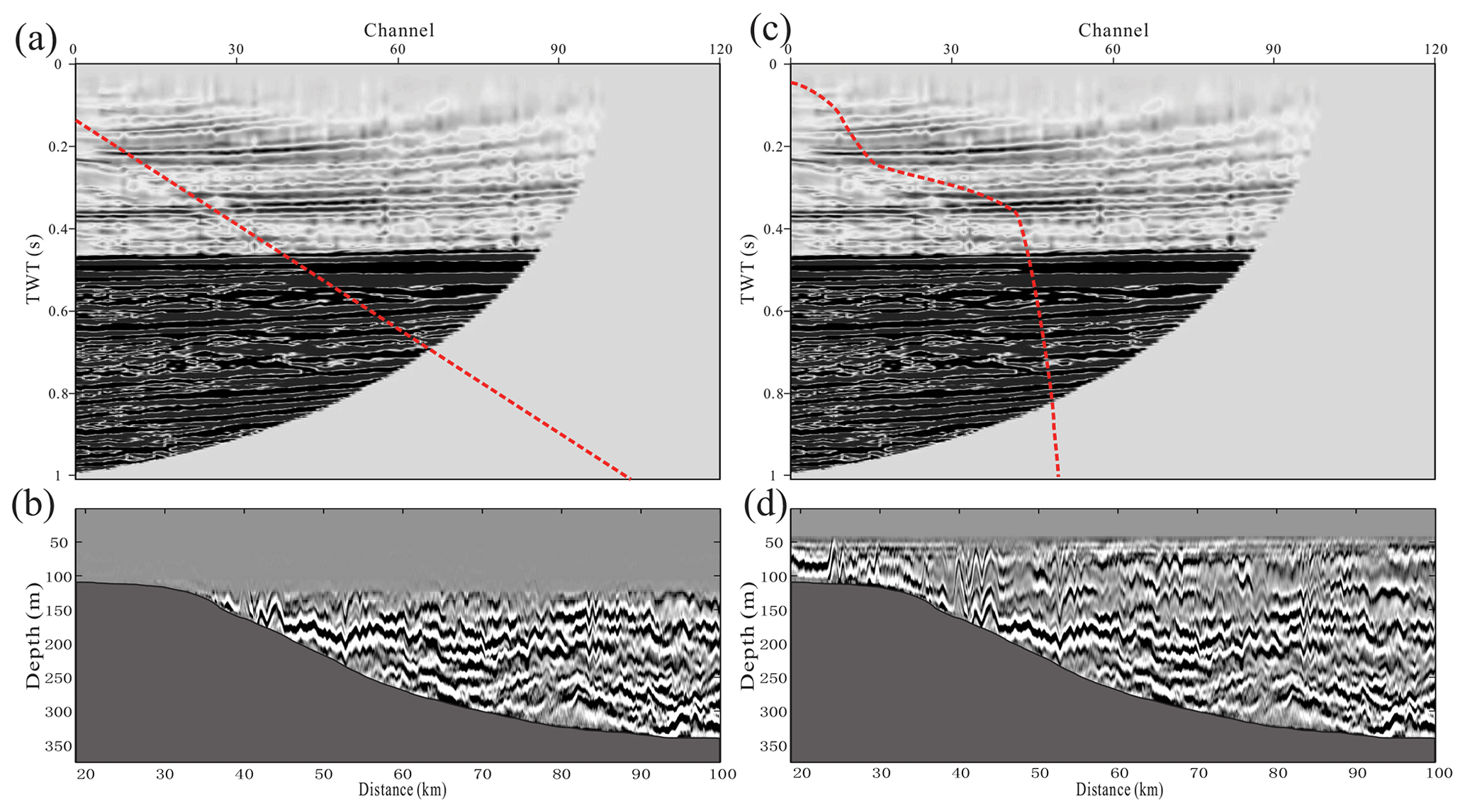
Figure 2Cutting off the stretch of NMO with a linear function (a) and the corresponding seismic section (b). Cutting off the stretch of NMO with a custom function (c) and the corresponding seismic section (d). The red dotted line shows the cutoff trace; the right part of seismic data is cut off. The unit TWT of (a) and (b) is the two-way travel time of seismic wave from source to receiver.
After a conventional processing of the seismic data, an image of the ocean interior's structure can be obtained. This image can be approximated as a temperature or salinity gradient map of the water column (Ruddick et al., 2009). The conventional processing of seismic data has five main steps, including defining the observation system, noise and direct wave attenuation, velocity analysis, normal moveout (NMO) and horizontal stacking. Then we use a bandpass filter to filter out low-frequency noise below 8 Hz and high-frequency noise above 80 Hz. According to the linear characteristics of the direct wave, we use a median filter to extract the direct wave signal and subtract it from the original signal to achieve the purpose of attenuating the direct wave. Subsequently, we sorted the seismic data from shot gathers into common midpoint gathers (CMPs). Sound speed is a function of depth and is obtained through velocity analysis, and then the NMO is applied to CMPs according to the function to flatten the reflection seismic events of the water column. When NMO is applied, the seismic wave with a large offset will be stretched, and the stretched seismic waves need to be cut off. Usually, the default method is to use a linear function to remove the stretched seismic waves (Fig. 2a). This may lose a lot of shallow reflection signals (Fig. 2b). Bai et al. (2017) used the common offset seismic section to supplement the missing information in shallow water, but the low signal-to-noise ratio of the common offset seismic section cannot guarantee the imaging quality. In order to retain more shallow reflection signal, we used a custom function to cut off the NMO stretch (Fig. 2c), thereby satisfying the imaging requirement of the shallow water column (Fig. 2d). Finally, the seismic section of the water column can be obtained by stacking the processed CMPs. Due to the shallow water depth, the seismic data are seriously affected by swell noise. We filtered out the components of stacked seismic data in the wavenumber range corresponding to swells in the frequency–wavenumber domain. A detailed description of the seismic data processing can be found in Ruddick et al. (2009).
2.2 Diapycnal diffusivity estimates from seismic data
Klymak and Moum (2007) found that the horizontal wavenumber spectrum of the vertical isopycnal displacement can be interpreted as the internal wave spectrum at low wavenumbers and the turbulence spectrum at high wavenumbers. The high wavenumber components of the spectrum are dominated by turbulence, and the spectral energy follows the power of the wavenumber. The turbulence part of the horizontal wavenumber spectrum can be expressed by a simplified Batchelor model (Eq. 1), so the turbulence dissipation ε can be estimated from the observed horizontal wavenumber spectrum, and diapycnal diffusivity can be calculated from Eq. (2) (Osborn, 1980).
where represents the horizontal wavenumber spectrum, Γ=0.2 is the mixing coefficient, N is the buoyancy frequency, CT=0.4 is the Kolmogorov constant, ε represents the turbulence dissipation, kx is the horizontal wavenumber, and Kρ represents the diapycnal diffusivity.
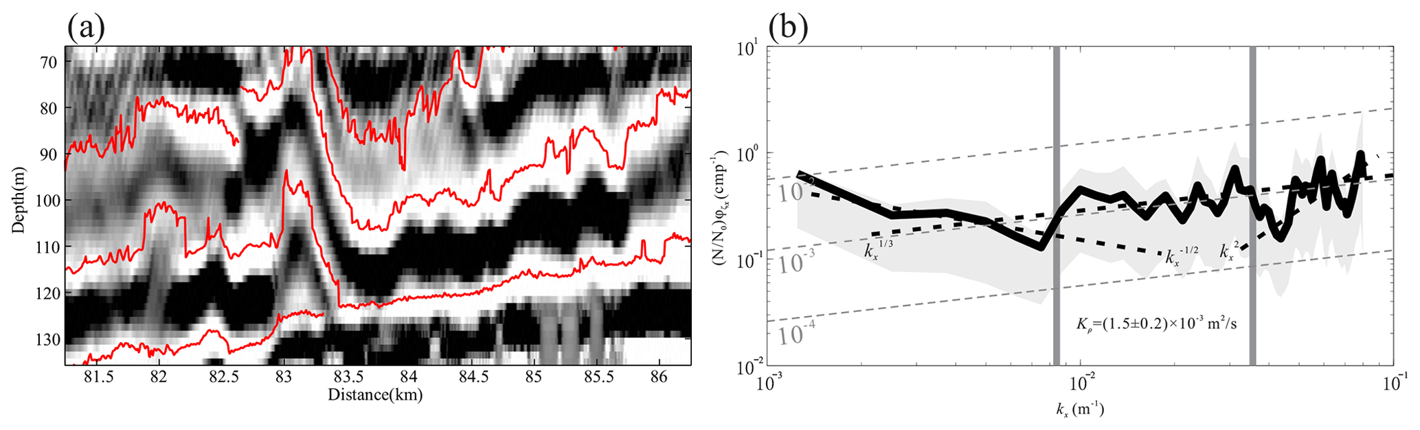
Figure 3(a) The reflection seismic events in a grid. (b) The average horizontal slope spectrum (black line). The gray shadow represents the 95 % confidence interval. The gray dashed lines represent the diffusivity contour. The black dashed lines represent the spectral slopes in the internal wave subrange, turbulence subrange and noise subrange, respectively. The gray vertical lines indicate the boundaries of the turbulence subrange.
Observations (Nandi et al., 2004; Nakamura et al., 2006; Sallarès et al., 2009) and simulations (Holbrook et al., 2013) show that the reflection seismic events and isopycnals are spatially consistent. Therefore, the horizontal wavenumber spectrum calculated from the vertical displacement of the reflection seismic events is equivalent to the horizontal slope spectrum that Klymak and Moum (2007) calculated from horizontal tow measurements. The turbulence dissipation and diapycnal diffusivity can also be calculated from seismic data (Sheen et al., 2009; Holbrook et al., 2013). First, we use the seismic interpretation software to pick up reflection events in the seismic section (Fig. 3a). Then we calculate the vertical displacement of the reflection events. The vertical displacement is the distance of the reflection events deviating from the equilibrium position in the vertical direction. We take the mean water depth of the reflection events as the equilibrium position. Note that the choice of equilibrium position will not affect the calculation result. The spectral energy of the vertical displacement in the horizontal wavenumber domain can be obtained by Fourier transform. In practical applications, we use the slope spectrum instead of the displacement spectrum to distinguish the turbulence subrange from the internal wave subrange. The spectral slope is as follows (Holbrook et al., 2013):
This conversion changes the wavenumber power law in the turbulence subrange from to , so that it can be distinguished from the internal wave subrange with the power law ( in the displacement spectrum). In calculating the turbulence dissipation in the seismic section, it is necessary to grid the section and calculate the dissipation in each grid separately. The horizontal grid is set as 5 km and the grid step as 2.5 km. As the water depth in the seismic data is shallow, the reflection seismic events are less in the vertical direction. In order to ensure more than two events in each grid, we set the vertical grid to be 75 m and the grid step to be 37.5 m. In each grid, we calculated the spectral slope of each event and took the average as . We fitted the averaged spectrum in the turbulence subrange to Eq. (1) and calculated the turbulence dissipation ε. To reduce uncertainty, we only calculated the cases with a length > 1000 m in each grid. Experiments showed that this length can correctly represent the slope of energy spectra in the turbulence subrange (Fig. 3b). After traversing all the grids, the turbulent dissipation section is obtained, and the diapycnal diffusivity section can be obtained as well according to Eq. (2). The uncertainty of the turbulence dissipation and diapycnal diffusivity was evaluated by the error between the observed average slope spectrum and the fitted Batchelor model (see Appendix). We used a spline smoothing function to smooth the meshing results.
2.3 Estimating the horizontal wave-induced velocity of internal solitary waves
We estimated the wave-induced horizontal velocity of internal solitary waves according to the method proposed by Moum et al. (2007a). This method requires the observational data to satisfy two assumptions: (1) the isopycnal is parallel to the streamline; (2) the internal solitary wave satisfies the Korteweg–de Vries (KdV) equation. Moum et al. (2007a) picked the isopycnal from the high-frequency acoustic section and fitted it with the KdV equation. The displacement equation of the isopycnal can be obtained, and the derivation of the displacement equation is the wave-induced velocity. Seismic data satisfy the first assumption. Although breaking induced polarity reversal of internal solitary waves close the streamlines, it is difficult to record reflection seismic data from those areas with a closed streamline at the resolution scale of seismic data. The regional density gradient recorded by the reflection events still exists, and the streamline is parallel to the isopycnal at this time, while areas with closed streamlines are strongly mixed and the density gradient weakens or even disappears, which cannot be recorded in seismic data. Unfortunately, the internal solitary waves we observed do not satisfy the second assumption. The KdV equation can simulate internal solitary waves with small amplitude and weak nonlinearity, but the polarity reversal of the large-amplitude internal solitary waves we observed cannot be simulated well. Here we did not use theoretical models to fit observations. Although there are studies using theory to successfully simulate the polarity reversal of internal solitary waves (Liu et al., 1998; Zhao, 2003), it is difficult to match theories and observations. We used the picked reflection seismic events to calculate the isopycnal displacement η(x,z) (Fig. 4b). η(x,z) is the distance that reflection seismic events deviate from the equilibrium position, which is determined by the mean depth of two shoulders of one internal solitary wave (Fig. 4a). We smoothed η(x,z) with a spline function identical to that used for smoothing turbulence dissipation, so that the resolution of wave-induced velocity is consistent with that of turbulence dissipation. Therefore, the stream function can be expressed as (Holloway et al., 1999)
where c is the phase velocity of internal solitary waves. c can be estimated from pre-stack seismic data (Tang et al., 2014, 2015; Fan et al., 2021). The seismic data are redundant, because we have made multiple observations of the same events, which allows us to study the movement of the water column. Specifically, after sorting the seismic data into CMPs (Sect. 2.1), we extracted traces with the same offset from CMPs to form common offset gathers (COGs). Multiple COGs can be obtained in the order of offset from small to large. The larger the offset, the lower the signal-to-noise ratio of the data. We selected the first five COGs to ensure the imaging quality. Pre-stack migration of COGs yields COG sections, which show images of the same water column at different times. Tracking the change in shot–receiver pairs at a certain reflection point yields the phase velocity (Fan et al., 2021). Figure 4c shows the change in the shot–receiver pairs of the internal solitary wave trough in the L1 survey line. The straight line represents the fitting line of the shot–receiver pairs. The average phase velocity of the internal solitary wave during the imaging time is , where dcmp is half of the trace interval, dts the time interval of the shot, and k the slope of the fitted line. After calculating the flow function according to Eq. (4), the wave-induced horizontal velocity can be expressed as
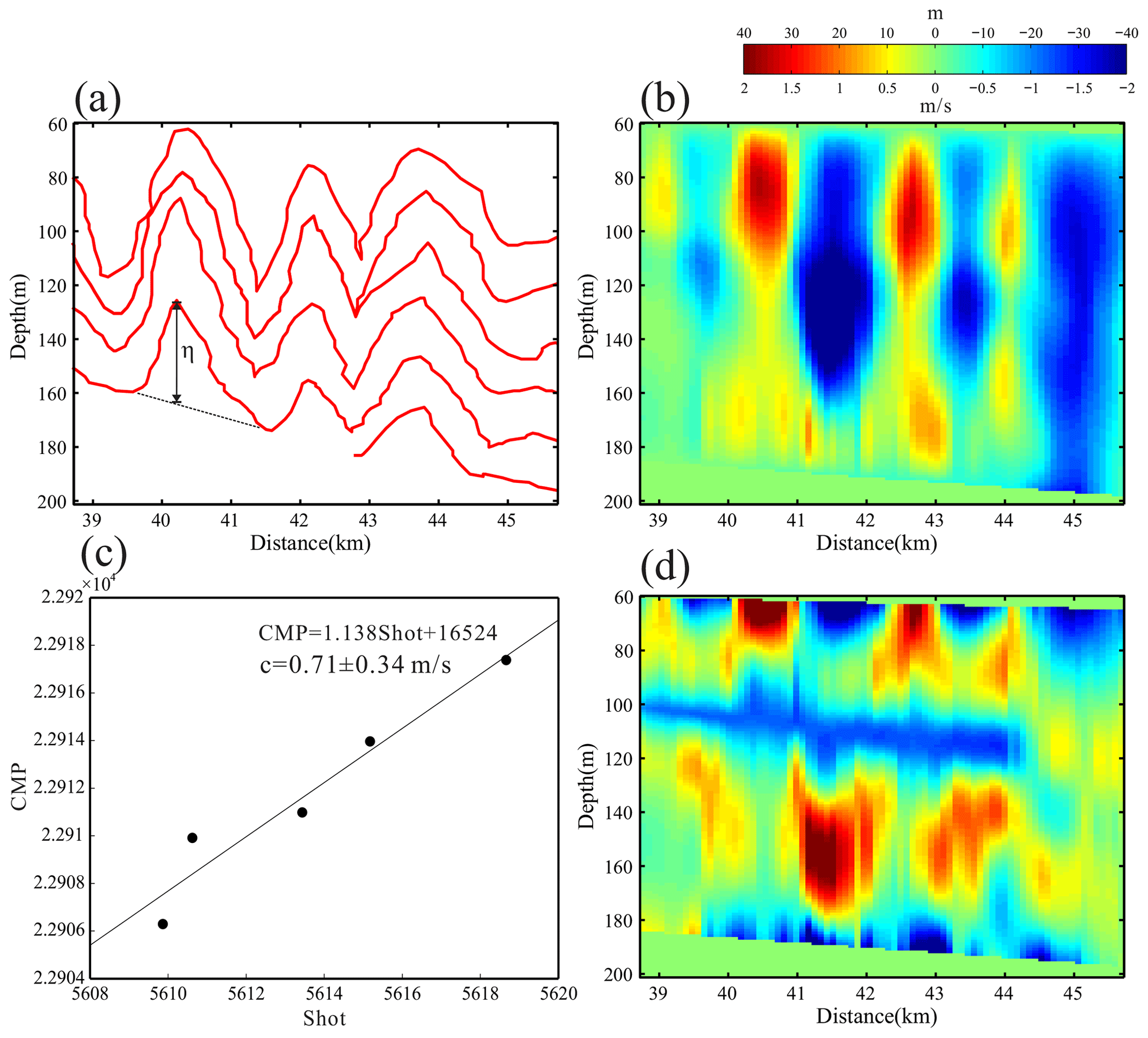
Figure 4(a) Schematic of calculating internal solitary wave isopycnal displacement using reflection seismic events. (b) The isopycnal displacement section of internal solitary waves. (c) Calculating the mean phase velocity of internal solitary waves by pre-stack seismic data. (d) The wave-induced horizontal velocity.
The wave-induced velocity here is on the seismic-resolution scale, which should be taken as its low-frequency component only. The results are insufficient to characterize the high-frequency components. However, this rough wave-induced velocity is useful, because our purpose in calculating wave-induced velocity is for the vertical mixing scheme. The wave-induced velocity makes the resolution scale of the mixing scheme equal to that of mixing parameters estimated from the seismic data, and the two are comparable. In addition, the error of the wave-induced velocity is mainly determined by the error of the phase velocity of the internal solitary wave. For internal solitary waves with polarity reversal, the error of the phase velocity is large, because the phase velocity gradually decreases when the internal solitary wave is shoaling (Bourgault et al., 2007; Shroyer et al., 2008). It can be seen from Fig. 4c that the shot–receiver pairs do not completely fall on the fitted line.
2.4 Mixing scheme for internal solitary wave shoaling
Shoaling and breaking of internal solitary waves on the continental shelf and slope enhance mixing. Vlasenko and Hutter (2002) studied the breaking of internal solitary waves over slope–shelf topography by numerical simulation. In their model, the mixing scheme (PP scheme) proposed by Pacanowski and Philander (1981) was improved, and a vertical mixing scheme for resolving breaking internal solitary waves was given. In this scheme, the vertical turbulence kinematic viscosity and diffusivity are determined by the Richardson-number-dependent turbulence parameterizations. The expression is as follows:
where uz is the vertical gradient of horizontal wave-induced velocity, ν is vertical turbulence kinematic viscosity, and κ is vertical turbulence kinematic diffusivity. Vlasenko and Hutter (2002) selected the best model parameters after a series of experiments. They are m2 s−1, m2 s−1, m2 s−1, α=5 and n=1. Based on this model, they simulated the process of internal solitary wave shoaling and breaking on slope–shelf topography and studied the breaking criterion.
3.1 Polarity reversal of internal solitary waves in the seismic section
When one internal solitary wave propagates across the transition point, it converts from a depression wave to an elevation wave. In the two-layer ocean model, the transition point is defined as the position where the pycnocline is close to the middle depth (Grimshaw et al., 2010). The three seismic sections in Fig. 5 capture the images of internal solitary waves passing the transition point. Figure 5a is the seismic section of survey line L1. It shows that the water depth becomes shallower from southeast to northwest, and the bottom slope is steeper between 30 and 60 km. In the deep-water region of 60–100 km, internal waves are developed, and the reflection seismic events fluctuate obviously. Near the seafloor around 80 km, the reflection seismic events are uplifted and discontinuous, forming a fuzzy reflection area. A mode-1 depression internal solitary wave can be identified at 53 km, indicating that the transition point has not been reached yet. The internal solitary wave has reversed polarity at 40 km, and a packet of three elevation waves is formed. The reflection seismic events are continuous here, implying no wave breaking. Five elevation waves can be identified around 24–37 km, among which four elevation waves at 24 km may be formed continuously, while the elevation wave at 37 km is formed later.
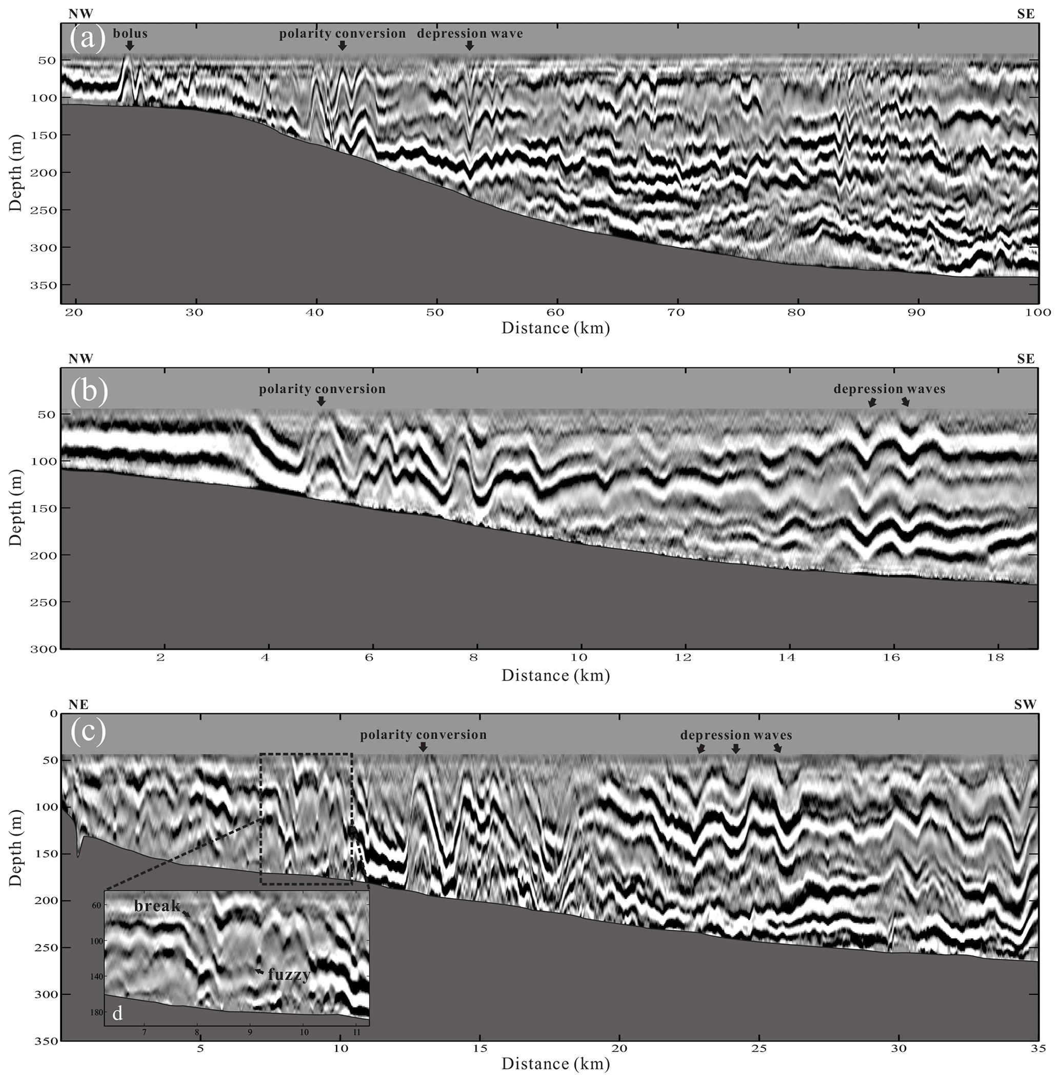
Figure 5The seismic sections of survey lines L1 (a), L2 (b) and L3 (c). The gray regions in the sections represent the seafloor. Internal solitary waves can be seen in all three cases. Panel (d) is the enlarged regional image of 6–10 km.
Figure 5b gives another internal solitary wave polarity reversal process captured by survey line L2. There are two obvious depression waves at 16 km. There are multiple waves with smaller amplitudes around 10–15 km. The polarity of internal solitary waves reverses within 4–8 km. The length of the head wave becomes wider and the slope becomes gentler. The leading wave is followed by a packet of multiple elevation waves. The reflection seismic events are continuous in the whole section.
L3 is a cross-line whose observation direction is perpendicular to survey lines L1 and L2 (Fig. 5c). There are multiple depression waves with large amplitudes of 20–35 km, and the reflection seismic events are continuous. The wave polarity is reversing within 10–20 km, and the reflection seismic events are discontinuous in this region. At 10 km, there is a large-amplitude elevation internal solitary wave, and the wave front is almost parallel to the seafloor. There is a large-amplitude depression wave at 17 km, and the wave trough has interacted with topography. Most of the reflection seismic events before 10 km are discontinuous and fuzzy, especially in the range of 6–10 km (Fig. 5d). It indicates that the reflective structures in this region may be destroyed by internal solitary wave breaking. It should be noted that the breaking mentioned in this article refers to local breaking caused by instability, not the four types of classic breaking (Aghsaee et al., 2010).
3.2 The horizontal slope spectrum
We picked the reflection seismic events in the three sections (Fig. 7) and calculated the horizontal slope spectrum using the method described in Sect. 2.2. Figure 6 shows the average horizontal slope spectrum of the three sections. We calculated the horizontal slope spectrum of all tracked events and averaged in logarithmic space to determine the wavenumber of the turbulence subrange. The turbulence subrange of the survey line L1 section is 0.005–0.069 m−1, as shown by the gray vertical line in Fig. 6a. The corresponding wavelength is 15–200 m. The average diapycnal diffusivity is (7.0 ± 1.2) × 10−4 m2 s−1, which is 1 order of magnitude larger than the open-ocean value (10−5 m2 s−1). The spectral energy in the internal wave subrange is larger than that in the turbulence subrange, indicating that the energy is dominated by internal waves. This is confirmed by internal waves in the seismic sections. The difference from Holbrook et al. (2013) is that the calculated horizontal slope spectrum does not include harmonic noise. This may be because harmonic noise has been removed when we filtered out the swell noise. In addition, we have not smoothed the events, so some high-wavenumber ranges are reserved. If the events are smoothed, the spectral energy will decrease rapidly in the high-wavenumber range (Holbrook et al., 2013; Tang et al., 2019).
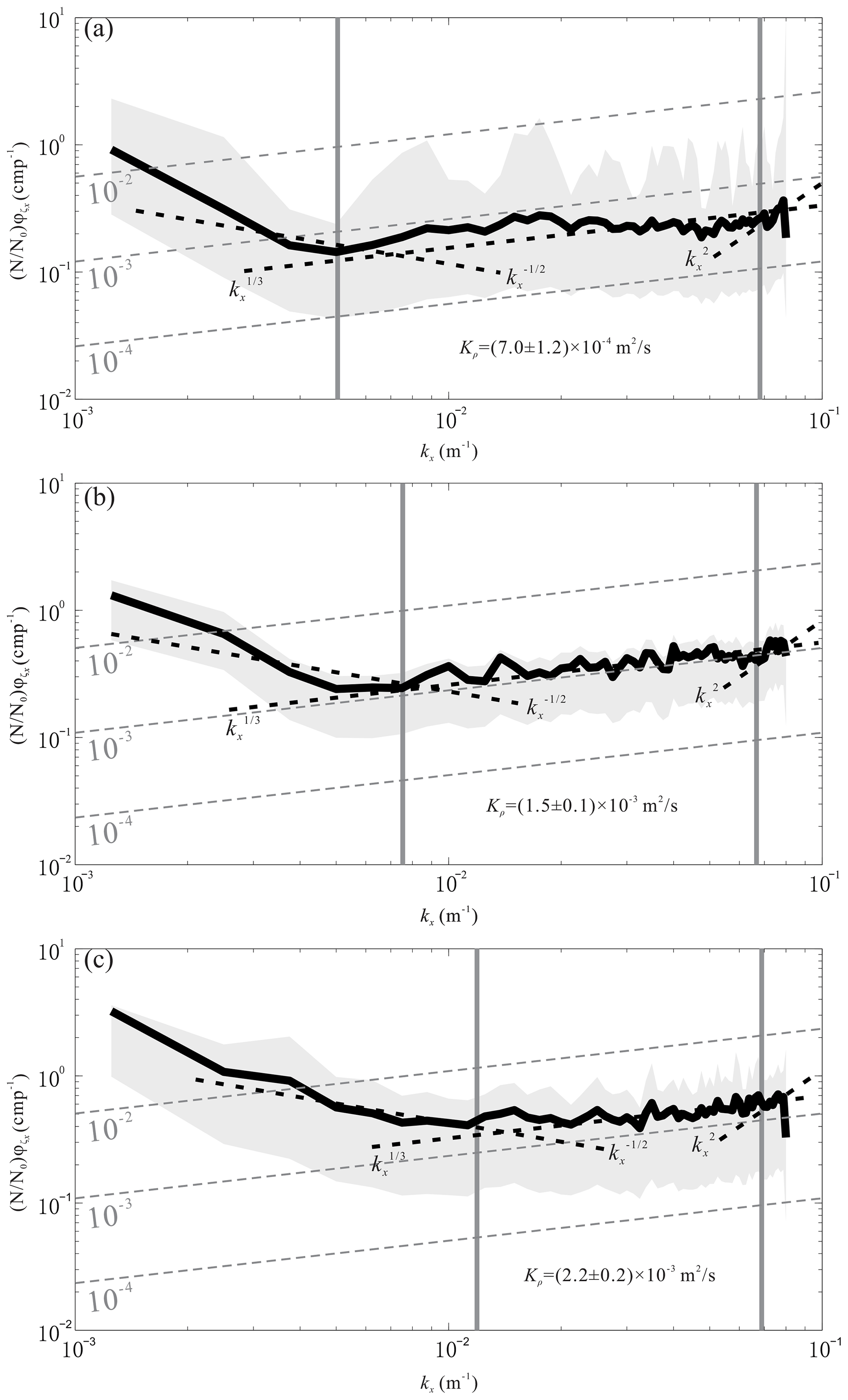
Figure 6The average horizontal slope spectra of the L1 section (a), L2 section (b) and L3 section (c). The black line is the spectrum, the gray shadow represents the 95 % confidence interval, the gray dashed lines represent the diffusivity contour, and the black dashed lines represent the spectral slopes in the internal wave subrange, turbulence subrange and noise subrange, respectively. The gray vertical lines label the boundaries of the turbulence subrange.
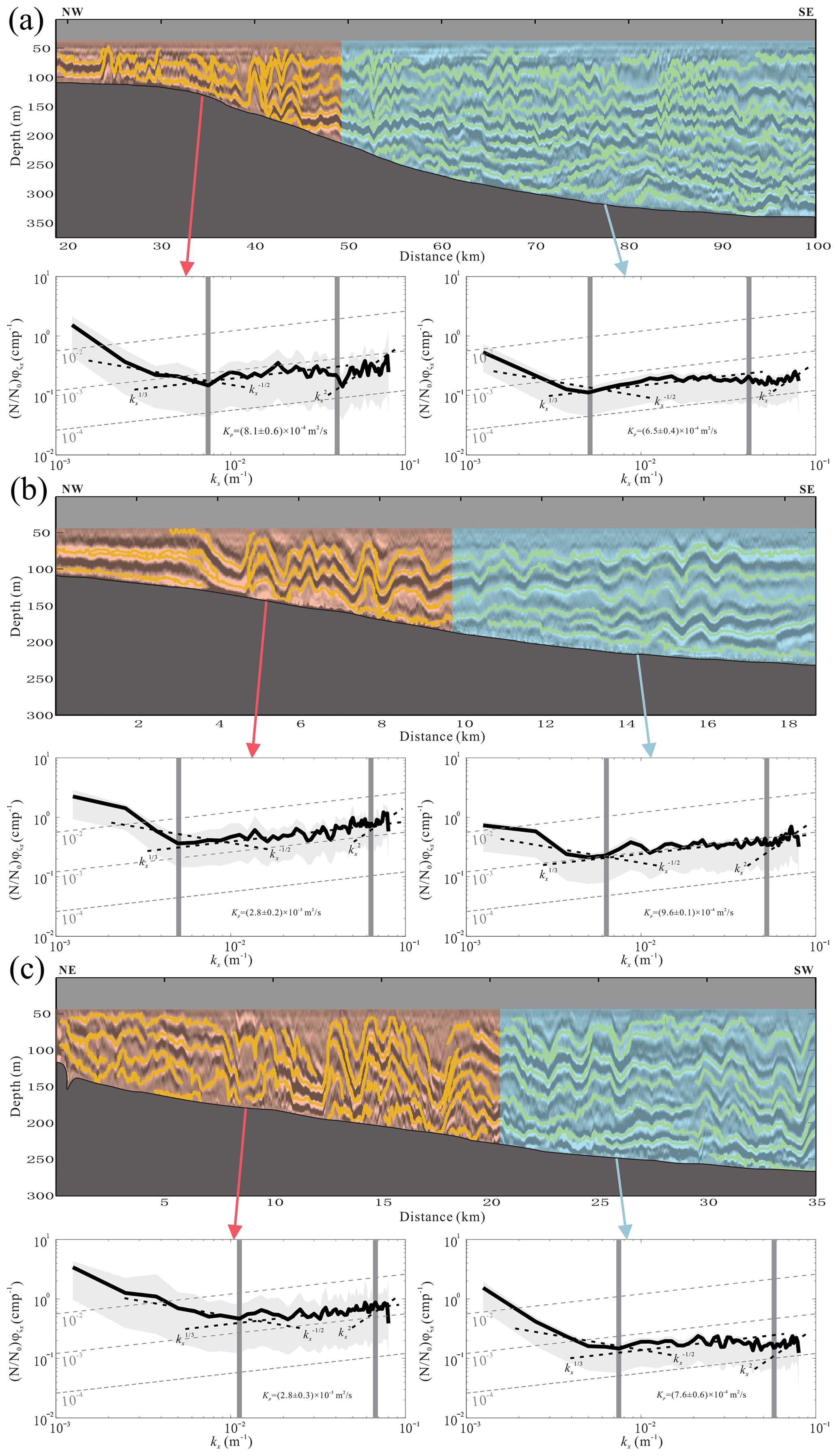
Figure 7The horizontal slope spectra of the polarity reversal and non-polarity reversal regions calculated from the L1 section (a), L2 section (b) and L3 section (c). The yellow lines are tracked reflection seismic events.
The horizontal slope spectrum of the L2 section is shown in Fig. 6b. The turbulence subrange is 0.008–0.068 m−1, and the corresponding wavelength is 15–133 m. Compared with survey line L1, the turbulence shifts to a smaller scale. The spectral energy in the internal wave subrange has the same order of magnitude as the spectral energy in the turbulence subrange, which indicates that the energy is transferring to small-scale turbulence. This process is closely related to the polarity reversal of internal solitary waves. The average diapycnal diffusivity is (1.5 ± 0.1) × 10−3 m2 s−1, which is 2 orders of magnitude larger than the background value.
Figure 6c is the horizontal slope spectrum of the L3 section. It can be seen from the spectrum that the turbulence subrange is small, ranging from 0.011 to 0.07 m−1. The corresponding wavelength is 14–89 m. The internal wave energy is larger and occupies a larger scale range. It can be seen from the seismic section of survey line L3 (Fig. 5c) that the wave amplitudes are large. It indicates that the internal waves carry more energy, so the spectral energy in the internal wave subrange is larger (Fig. 6c). In addition, there are many discontinuous and weak reflections in the seismic section caused by breaking internal solitary waves. Internal solitary wave breaking weakens the density gradient and enhances local mixing. This phenomenon is most typical in survey line L3, where the average diffusivity (2.2 ± 0.2) × 10−3 m2 s−1 is the largest of the three sections.
Figure 6 shows that the spectral energy of the L1 section is smaller than that of the other two sections. This may be because the imaging range of the L1 section is different. The observations in the L2 and L3 sections are the polarity reversal of internal solitary waves, while the L1 section includes not only the polarity reversal process, but also internal waves in deep water. The spectral energies of these two processes should be different. We calculated the average horizontal slope spectrum of the polarity reversal region and the non-polarity reversal region, respectively (Fig. 7). The spectral energy of the polarity reversal region in the L1 section is higher than that of the non-polarity reversal region, and so does diapycnal diffusivity (Fig. 7a). It implies that the wave energy will accelerate to dissipate and transfer to turbulence when its polarity is reversed. Compared with the non-polarity reversal region, the turbulence subrange of the polarity reversal region is smaller. The lower boundary of the turbulence subrange of the polarity reversal region is slightly larger than that of the non-polarity reversal region. It indicates that the turbulence in this region has a smaller scale. The diapycnal diffusivity in the polarity reversal region in the L2 section is about 3 times that of the non-polarity reversal region (Fig. 7b). The turbulence subrange of the polarity reversal region in the L2 section is slightly larger than that of the non-polarity reversal region. From the L2 section, it can be seen that the events are continuous during the polarity reversal process, which indicates that the wave breaking is weak. The internal solitary wave gradually fissions into several tails during the polarity reversal, and energy is dissipated constantly. Therefore, there will be a large turbulence subrange in the lateral direction (Fig. 7b). This process can dissipate much more energy compared with direct breaking of internal solitary waves (Masunaga et al., 2019). The diapycnal diffusivity in the polarity reversal region in the L3 section is larger, more than 3 times that of the non-polarity reversal region. Although there are more internal (solitary) waves with larger amplitude in the non-polarity reversal region, the diapycnal diffusivity is lower. The polarity reversal of internal solitary waves significantly increases the diapycnal diffusivity. The turbulence subrange of the polarity reversal region is small, and the lower boundary of the turbulence subrange is greater than 0.01 m−1.
3.3 Diapycnal diffusivity maps
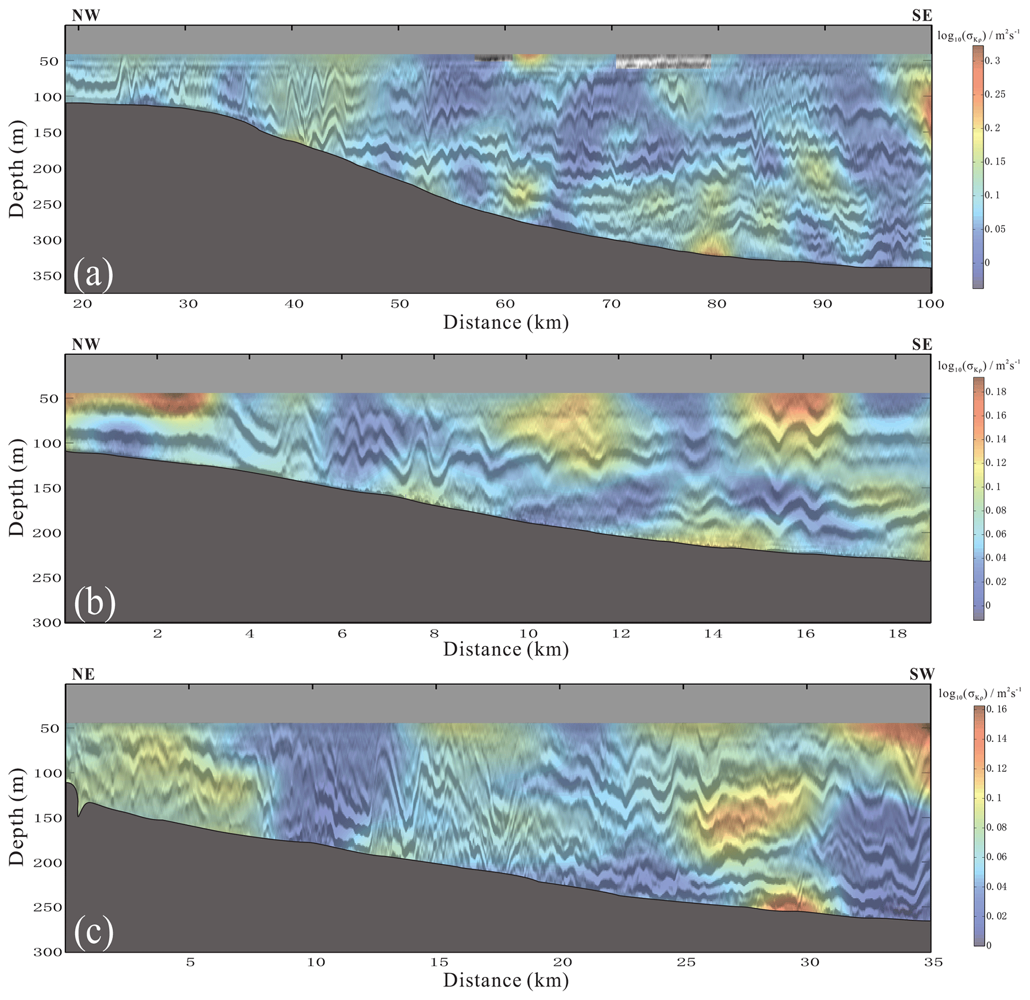
The diapycnal diffusivity maps of the three survey lines are shown in Fig. 8. Figure 8a shows the map of survey line L1. The diffusivity is higher than that of the open ocean. The high value presents a patchy distribution, mainly distributed in the depth between 50 and 150 m. The low-diffusivity values are mainly distributed in the depth between 150 and 300 m. Some high values are also distributed near the seafloor. The diffusivity is larger in the polarity reversal region (24–45 km). Compared with the diffusivity of the four adjacent elevation internal solitary waves (24–30 km), we find that the diffusivity is proportional to the amplitudes of internal solitary waves. It means that the large-amplitude internal solitary waves contribute more to mixing. In the polarity reversal region (40–45 km), the diffusivity of the head wave's front is higher, that is, where the slope of the wave front becomes gentle, while the diffusivity of the two elevation waves following the head wave is small. It indicates that the mixing induced by internal solitary wave polarity reversal is stronger at the beginning, and more energy is dissipated at this time. In the non-polarity reversal region (50–100 km), the diffusivity is low. The mode-1 depression internal solitary wave at 52 km increases the diffusivity. There is an abnormal reflection area near the seafloor at 80 km, and the diffusivity is high. In addition, there is also an area with increased diffusivity between 100 and 250 m at 93 km. This may be related to large-amplitude internal waves.
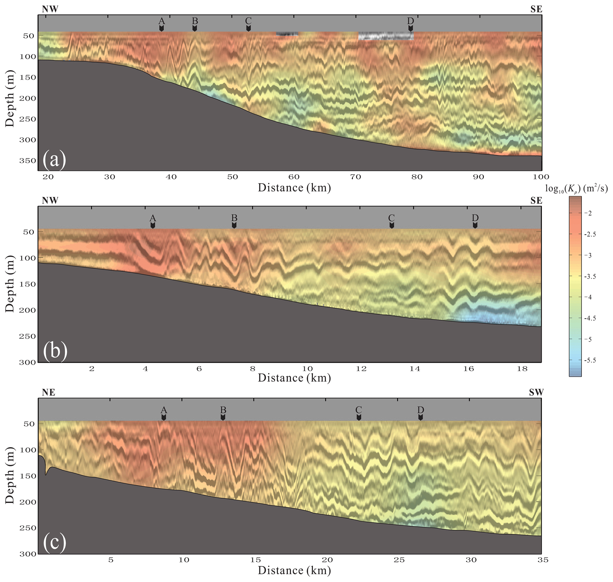
Figure 8The diapycnal diffusivity map of survey lines L1 (a), L2 (b) and L3 (c). The black arrows represent the positions of vertical diffusivity profiles.
The diffusivity map of survey line L2 is shown in Fig. 8b. The high value is mainly distributed at the front of the head wave during the polarity reversal process (4 km), which is consistent with the characteristics on L1. The diffusivity after the head wave is low, but it is still higher than that in other regions. The diffusivity in the non-polarity reversal region is almost uniform. The two internal solitary waves at 15–16 km did not increase the diffusivity. There is a low-diffusivity area near the seafloor around 16–18 km, which is caused by untracked reflection seismic events in this area. The diffusivity map of survey line L3 (Fig. 8c) is similar to that of L2. The high value is distributed in the polarity reversal region, and the diffusivity of the head wave is still high. However, unlike the diffusivity map of L2, the high diffusivity is mainly distributed in the shallow part of the head wave (water depth 50–120 m), while the diffusivity of the whole head wave in L2 is high. In the non-polarity reversal region, the diffusivity is small and the distribution is uniform too. The diffusivity near the seafloor at 25–27 km is slightly lower than other regions.
4.1 The relationship between diffusivity and reflection seismic events
When there is a significant impedance difference in the water column, a reflection seismic event will occur (Holbrook et al., 2003; Ruddick et al., 2009). The impedance difference in the ocean is contributed by temperature gradient and salinity gradient, where the former is usually greater than the latter (Ruddick et al., 2009; Sallarès et al., 2009). Density is a function of temperature and salinity, so the reflection seismic events are related to density gradient. The enhanced mixing reflects the structure of density gradient, thereby changing the appearance of the reflection seismic events. Understanding the relation between diffusivity and reflection seismic events can help us analyze the spatial distribution of diapycnal mixing. Figure 8 shows that the reflection seismic event in the high-diffusivity region is obviously different from that in the low-diffusivity region. In the high-diffusivity area (red in Fig. 8), the reflection seismic events are fuzzy, discontinuous or bifurcate, while in the low-diffusivity area (yellow and blue in Fig. 8), the reflection seismic events are clear and continuous. This is because regions with high diffusivity are strongly mixed. The density gradient is smeared by mixing, so that it affects the appearance of reflection seismic events. For example, in the polarity reversal region of three seismic sections, the diffusivity is high and the reflection seismic events are fuzzy and discontinuous. Especially in the range of 5–10 km in Fig. 8c, the events are obviously broken and weak. The diffusivity is low in areas where the events are clear, such as the region near the seafloor around 45–50 km and the region near the seafloor around 93–99 km in Fig. 8a and the region near the seafloor around 24–27 km in Fig. 8c.
The diffusivity is not only related to the continuity of the reflection events, but is also related to the fluctuation intensity of the events. The greater the fluctuation intensity of the events, the higher the spectral energy and the greater the diffusivity value. There is a mode-1 depression internal solitary wave at 50–58 km in Fig. 8a, and the reflection seismic event is clear and continuous at 180 m. However, the diffusivity is high, because the reflection events fluctuate more strongly. It can be seen from the figure that, in addition to the amplitude of the internal solitary wave, there are also many high-frequency waves at the shoulders of the internal solitary wave. These waves increase the spectral energy and result in a higher diffusivity. In addition, the reflection seismic events before 4 km in Fig. 8b are continuous and without obvious fluctuations, but the diffusivity is higher. It can be seen from the figure that the reflection events of this region are thicker than those of other regions. The seismic data processing of the three sections in Fig. 8 is the same, so the thicker events in Fig. 8b do not stem from the low frequency of seismic waves. We think this may be caused by small-scale mixing between layers, such as Kelvin–Helmholtz (K-H) instability. Figure 9 is an enlarged view of 2–3 km in the seismic section of L2 (Fig. 5b). The wavelength of the seismic wave (red line) at 80 m is larger than that at the seafloor, which is formed by the overlap of multiple wavelets. It can be seen from the figure that a weak reflection event is barely visible at 80 m, which indicates a thin reflection layer with weak impedance differences. The K-H instability can last for a long distance in the lateral direction (Seim and Gregg, 1994; Haren et al., 2014; Chang et al., 2016; Tu et al., 2019) and enhance local ocean mixing. This structure can form at the tail of internal solitary waves (Moum et al., 2003). The vertical scale of the K-H instability is small and usually appears on the isopycnal. On the one hand, K-H instability weakens the density gradient, so that the reflected seismic wave energy is reduced. On the other hand, the vertical scale of K-H instability is lower than the seismic wave resolution (a quarter of the seismic wave wavelength), so it causes overlapped wavelets and stretched wavelengths (Fig. 9). Therefore, the reflection event in this area is thicker. In addition, the horizontal scale of the K-H instability train is large, which may explain the larger turbulence subrange on the horizontal slope spectrum (Fig. 7b).
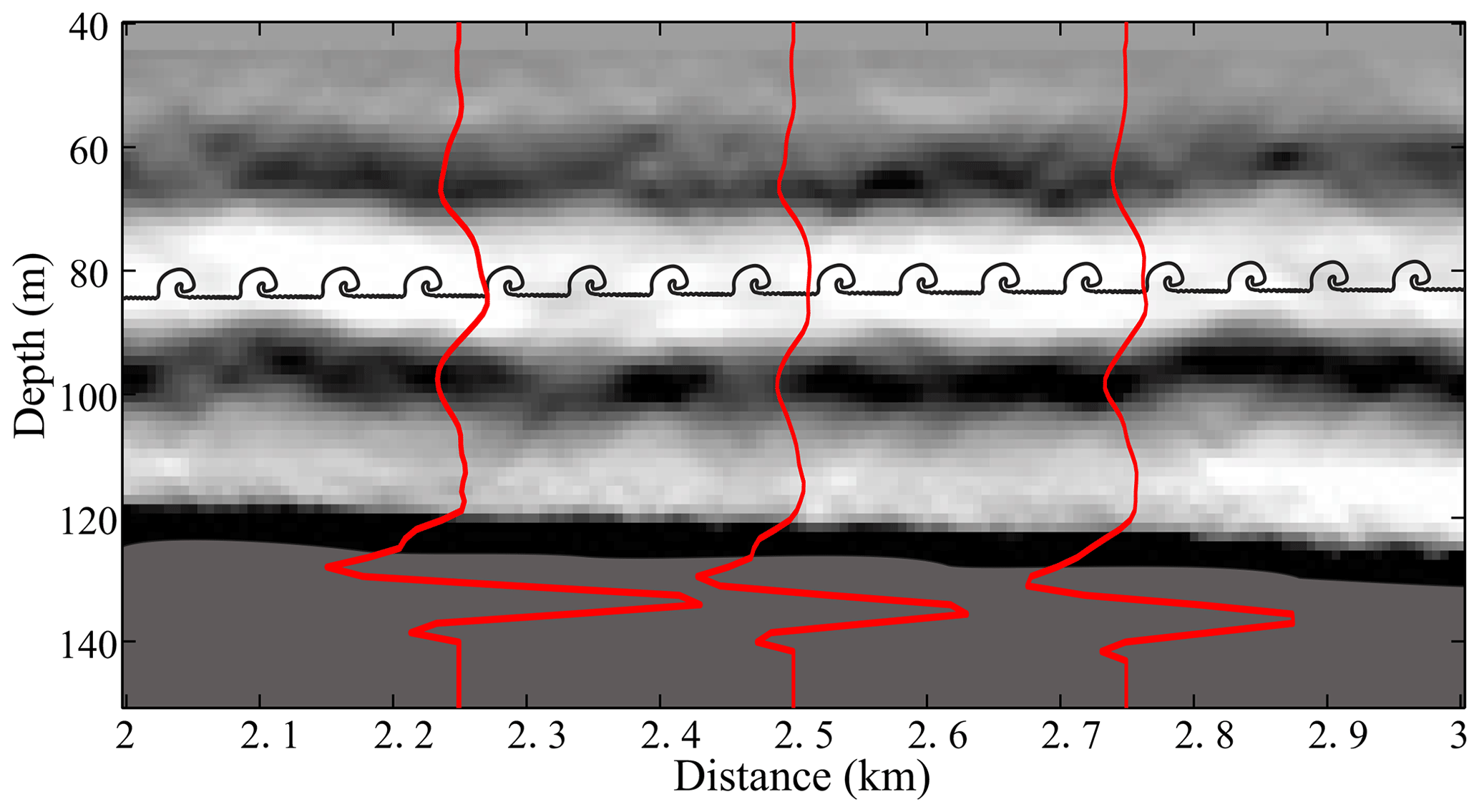
Figure 9Schematic of the K-H instability. The red lines are the seismic waves, and the black billows represent the K-H instability.
4.2 Enhanced diapycnal mixing induced by the polarity reversal of internal solitary waves
Strong mixing in the ocean mainly occurs near rough topography or areas with strong tides (Simpson et al., 1996; Rippeth et al., 2001, 2003; Nash and Moum, 2001; Klymak et al., 2008; Jarosz et al., 2013; Staalstrøm et al., 2015; Wijesekera et al., 2020; Voet et al., 2020). The Dongsha Atoll region in the South China Sea possesses both features. On the one hand, the Dongsha Atoll lies on the continental slope with variable topography. On the other hand, large-amplitude internal solitary waves (Alford et al., 2015) propagating from the Luzon Strait reflect, refract, and shoal in this region. This process will dissipate most of the energy carried by the internal solitary waves. Especially in the shoaling process, polarity reversal and breaking occur and the energy of internal solitary waves transfers to smaller-scale waves. Our results (Fig. 6) indicate that the average diffusivity has a magnitude order of O(10−4)–O(10−3) m2 s−1, consistent with previous observations by other techniques. St. Laurent (2008) observed turbulent mixing on the continental shelf and slope and found that the mixing is higher at the shelf break, and the magnitude order of average dissipation is O(10−7)–O(10−6) m2 s−1. According to the average buoyancy frequency N=6 cph, the magnitude order of the average diffusivity is O(10−4)–O(10−3) m2 s−1 and is consistent with our result. Yang et al. (2014) observed diapycnal mixing on the continental shelf and slope and found that the average diffusivity can reach O(10−3) m2 s−1 too. Similar results have been reported in the study of internal solitary waves shoaling in other regions. For example, Sandstrom et al. (1989) observed the turbulent diffusivity caused by the nonlinear internal wave group on the continental slope of Canada and found an average diffusivity of 2.4 × 10⁻³ m2 s−1. Carter et al. (2005) observed the elevation internal solitary waves in Monterey Bay and a diffusivity on the magnitude order of O(10−4) m2 s−1. Richards et al. (2013) observed the shoaling of nonlinear internal waves at the St. Lawrence Estuary, which induced high turbulence and enhanced mixing. Therefore, it is reasonable that diapycnal mixing induced by nonlinear internal waves on the continental shelf and slope in the northern South China Sea can reach 100 times that in the open ocean.
The high diffusivity is mainly in the leading internal solitary wave during the polarity reversal. We suggest that strong mixing may be caused by internal wave breaking due to convective instability. In Fig. 8a and c, the reflection seismic events are obviously discontinuous in the high-turbulence area, indicating that the density gradient is weakened by internal wave breaking. The trough of the internal solitary wave decelerates first when the polarity is reversed (Shroyer et al., 2008), which makes the Froude number (Fr) greater than 1 and causes convective instability. This phenomenon can be found in other observational data. In the high-frequency acoustic section, the backscatter at the top of an internal solitary wave is increased when it changes from depression to elevation wave (Orr and Mignerey, 2003), which indicates that the turbulence of the front increased. However, in the seismic section of Fig. 8b, we did not find breaking at the front of the polarity reversal internal solitary wave. The strong mixing of this internal solitary wave may be induced by shear instability (Fig. 9). Therefore, both convective instability and shear instability are responsible for the enhanced mixing in this process. In addition, the non-polarity reversal region in Fig. 8a has a higher diffusivity in 50–150 m than other regions. This range is in the thermocline (Fig. 1c). The internal waves usually greatly increase mixing in the thermocline, which is related to shear instability of internal waves (MacKinnon and Gregg, 2003). Shear instability is an important mechanism of internal wave dissipation (Farmer and Smith, 1978), and it more likely occurs in nonlinear internal waves than convective instability (Zhang and Alford, 2015). The results of high-frequency acoustic observations show that the enhanced backscatter at the bottom of the thermocline represents higher shear instability when the internal solitary waves are shoaling (Orr and Mignerey, 2003), which is consistent with the depth range of high diffusivity in our results.
What is inconsistent with the observed distribution of mixing is that our results do not show diffusivity in the bottom boundary layer. Because our seismic data were collected in summer, the strong stratification at this time limits the vertical range of the bottom boundary layer (MacKinnon and Gregg, 2003), so that the bottom boundary layer near the Dongsha Atoll is thin and lower than the thickness that can be recorded by seismic data. So, the diffusivity we calculated does not include the bottom boundary layer. The enhanced diapycnal mixing induced by the polarity reversal of internal solitary waves plays an important role in local environment and primary productivity. On the one hand, diapycnal mixing on the continental slope and shelf makes an important contribution to ocean heat flux, which affects climate and the ocean through heat exchange of the local water column (Rahmstorf, 2003; Tian et al., 2009). On the other hand, the vertical flux caused by turbulence can redistribute materials in the ocean and have an important impact on the marine ecological environment (Sharples et al., 2001; Moum et al., 2003; Klymak and Moum, 2003; Wang et al., 2007).
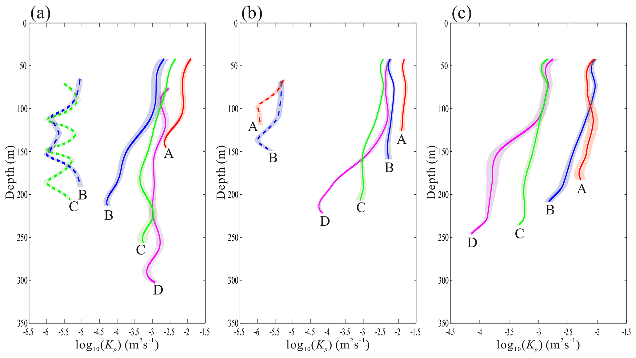
Figure 10The vertical distribution of diffusivity from seismic data compared with the mixing scheme. The solid line represents the vertical distribution of diffusivity at the four positions A (red), B (blue), C (green) and D (magenta), and the dotted line represents the parameterized diffusivity at the corresponding positions. The shadow indicates the margins of errors.
4.3 The mixing scheme of internal solitary wave shoaling
We compared the vertical distribution of diffusivity with the vertical mixing scheme of internal wave breaking proposed by Vlasenko and Hutter (2002). Although Klymak and Legg (2010) also proposed a mixing scheme for internal wave shoaling and achieved good results in numerical simulation, we cannot use that method to calculate mixing parameters because of lacking high-resolution density observation data. Figure 10 shows the vertical distribution of diffusivity from seismic data (solid line) and the diffusivity calculated from a mixing scheme (dashed line) at four positions of the three survey lines (black arrows in Fig. 8). The reflection events in the L3 section are broken, and it cannot be guaranteed that the events are parallel to the streamline. Therefore, we did not use the method described in Sect. 2.3 to calculate the wave-induced velocity and thus did not obtain the diffusivity of the mixing scheme. It can be seen from Fig. 10 that the turbulent diffusivity gradually decreases from shallow to deep water. Except for the local low-diffusivity value in the deep water at position D of Fig. 10b and c, the diffusivity reduction rate at other locations is similar. Figure 10a and b show that the parameterized diffusivity is nearly 2–3 orders of magnitude smaller than our result, but they have a similar trend of change. In Fig. 10a (line L1), the parameterized diffusivity (blue dotted line) at position B decreases by an order of magnitude within 50–100 m. This tendency is the same as our results. However, the parameterized diffusivity within 150–200 m increases by 1 order of magnitude, which is inconsistent with our results (solid blue line). The parameterized diffusivity at position C fluctuates and keeps a decreasing trend on the whole. In survey line L2, we selected position A and position B to calculate the parameterized diffusivity. The diffusivity at position A (red dashed line) decreases rapidly within 60–100 m and then almost stays unchanged. This is different from our result (solid red line), and the reduction rate of the diffusivity is larger than our result. The trend of the diffusivity at position B (blue dashed line) above 110 m is consistent with our results (solid blue line), but the diffusivity below 110 m decreases rapidly and then rises again. In our results, the diffusivity decreases slowly at the same depth. The value is consistent with that in the open ocean. However, the mixing enhanced obviously on the continental shelf and slope because of the internal wave shoaling. The mixing scheme underestimates mixing, especially the strong mixing induced by the polarity reversal of internal solitary waves. Our results indicate that near the Dongsha Atoll, where large-amplitude internal solitary waves develop, mixing will be enhanced by the shoaling internal solitary waves. The diffusivity gradually decreases from shallow to deep water (not including the bottom boundary layer). This has important implications for improving the mixing scheme for models on the continental shelf and slope.
We have observed the polarity reversal of internal solitary waves by reflection seismic data near the Dongsha Atoll in the South China Sea and calculated their slope spectra (Fig. 6) and diapycnal diffusivity (Fig. 8). The results show that the average diapycnal diffusivities of the three survey lines are about 2 orders of magnitude greater than the open-ocean value. We calculated the average spectral slope of the polarity reversal and non-polarity reversal regions (Fig. 7) and found that the former is about 3 times larger than the latter. The diffusivity maps reveal that horizontally high diffusivity is mainly in the leading wavefront of an internal solitary wave in reversing polarity, and vertically high diffusivity is mainly in the thermocline (50–100 m).
We analyzed the relation between reflection seismic events and diapycnal diffusivity. The result indicates that continuous and clear reflection events correspond to low diffusivity, while discontinuous or fuzzy events correspond to high diffusivity. The strength of the events also affects the magnitude of diffusivity. The stronger the fluctuation, the higher the spectral energy and the higher the diffusivity. In addition, we observed an area of high diffusivity with a large horizontal scale in L2, and the reflection events did not appear to be discontinuous or fuzzy. We suggest that this enhanced mixing may be induced by the K-H instability (Fig. 9). The vertical scale of the K-H instability is smaller than the resolution of our seismic data, so we cannot observe clearly in the seismic data. However, its high-energy characteristics can be recorded by reflection events.
Our results show that shoaling internal solitary waves enhance local mixing. The magnitude order of diapycnal diffusivity is consistent with previous studies. We suggest that there are two mechanisms that could account for the enhanced mixing. On the one hand, the polarity reversal of internal solitary waves results in convection instability, which induces internal solitary wave breaking. This mechanism appears at the leading edge of one internal solitary wave in survey lines L1 and L3. The discontinuous reflection events indicate that the internal solitary wave is broken, while in the seismic section of L2, the reflection events are continuous and clear at the leading edge of the internal solitary wave and other strong mixing areas in the three sections. Such strong mixing may be caused by shear instability.
We picked four positions from the diffusivity maps to analyze the vertical distribution of diapycnal diffusivity (Fig. 10). Our result shows that the diffusivity gradually decreased from shallow to deep water (excluding the bottom boundary layer). Compared with one previous mixing scheme, the parameterized diffusivity is about 2–3 orders of magnitude smaller. This means that the mixing scheme underestimates mixing induced by internal solitary wave shoaling near the Dongsha Atoll. However, the vertical pattern of the parameterized diffusivity is consistent with our result.
According to Eqs. (1) and (2), the parameters used in calculating diffusivity are buoyancy frequency (N), mixing coefficient (Γ), and the Kolmogorov constant (CT). It can be seen from the formula that the diffusivity is proportional to N. The mean deviation of N we used is about 2 % (Fig. 1), so the uncertainty of the corresponding diffusion rate is about 0.008 logarithmic units. In addition, diffusivity is proportional to , which is 0.1–0.4 (Mashayek et al., 2017), so the corresponding uncertainty of diffusivity is about 0.15 logarithmic units. Similarly, diffusivity is proportional to . The value of CT is 0.3–0.5 (Sreenivasan, 1996), and the corresponding diffusivity uncertainty is about 0.15.
In addition, the key reason for the uncertainty of diffusivity in our calculation is the fitting of the Batchelor model and the slope spectrum (Figs. 3b and 6). We evaluated the uncertainty based on the least-squares standard deviation between the Batchelor model and the slope spectrum. The uncertainty of the three diffusivity maps in Fig. 8 is shown in Fig. A1.
The bathymetry data (https://www.gebco.net/data_and_products/gridded_bathymetry_data/) were provided by the General Bathymetric Chart of the Oceans (GEBCO Compilation Group, 2021) and prepared using the Generic Mapping Tools (https://www.generic-mapping-tools.org/, Wessel et al., 2019). The hydrological data sets (https://resources.marine.copernicus.eu/product-detail/GLOBAL_REANALYSIS_PHY_001_030, last access: 2 November 2020) we used were produced by the Copernicus Marine Environment Monitoring Service. The seismic data were processed using Seismic Unix (https://nextcloud.seismic-unix.org/s/LZpzc8jMzbWG9BZ, Stockwell, 1999).
The concept of this study was developed by HS and extended upon by all involved. YiG implemented the study and performed the analysis with guidance from HS. ZZ, YoG, KZ, YK and WF collaborated in discussing the results and composing the manuscript.
The contact author has declared that neither they nor their co-authors have any competing interests.
Publisher's note: Copernicus Publications remains neutral with regard to jurisdictional claims in published maps and institutional affiliations.
This article is part of the special issue “Nonlinear internal waves”. It is not associated with a conference.
The seismic data are owned by the Guangzhou Marine Geological Survey (GMGS). Thanks to the GMGS for providing two-dimensional seismic data.
This research has been supported by the National Natural Science Foundation of China (grant no. 41976048) and the National Key Research and Development Program of China (grant no. 2018YFC0310000).
This paper was edited by Kateryna Terletska and reviewed by two anonymous referees.
Aghsaee, P., Boegman, L., and Lamb, K. G.: Breaking of shoaling internal solitary waves, J. Fluid Mech., 659, 289–317, https://doi.org/10.1017/S002211201000248X, 2010.
Alford, M. H., Peacock, T., MacKinnon, J. A., Nash, J. D., Buijsman, M. C., Centurioni, L. R., Chao, S.-Y., Chang, M.-H., Farmer, D. M., Fringer, O. B., Fu, K.-H., Gallacher, P. C., Graber, H. C., Helfrich, K. R., Jachec, S. M., Jackson, C. R., Klymak, J. M., Ko, D. S., Jan, S., Shaun Johnston, T. M., Legg, S., Lee, I.-H., Lien, R.-C., Mercier, M. J., Moum, J. N., Musgrave, R., Park, J.-H., Pickering, A. I., Pinkel, R., Rainville, L., Ramp, S. R., Rudnick, D. L., Sarkar, S., Scotti, A., Simmons, H. L., St Laurent, L. C., Venayagamoorthy, S. K., Wang, Y.-H., Wang, J., Yang, Y. J., Paluszkiewicz, T., and Tang, T.-Y.: The formation and fate of internal waves in the South China Sea, Nature, 521, 65–69, https://doi.org/10.1038/nature14399, 2015.
Bai, Y., Song, H., Guan, Y., and Yang, S.: Estimating depth of polarity conversion of shoaling internal solitary waves in the northeastern South China Sea, Cont. Shelf Res., 143, 9–17, https://doi.org/10.1016/j.csr.2017.05.014, 2017.
Bogucki, D., Dickey, T., and Redekopp, L. G.: Sediment resuspension and mixing by resonantly generated internal solitary waves, J. Phys. Oceanogr., 27, 1181–1196, https://doi.org/10.1175/1520-0485(1997)027<1181:SRAMBR>2.0.CO;2, 1997.
Bourgault, D., Blokhina, M. D., Mirshak, R., and Kelley, D. E.: Evolution of a shoaling internal solitary wavetrain, Geophys. Res. Lett., 34, L03601, https://doi.org/10.1029/2006gl028462, 2007.
Cai, S., Xie, J., and He, J.: An overview of internal solitary waves in the South China Sea, Surv. Geophys., 33, 927–943, https://doi.org/10.1007/s10712-012-9176-0, 2012.
Carter, G. S., Gregg, M. C., and Lien, R.-C.: Internal waves, solitary-like waves, and mixing on the Monterey Bay shelf, Cont. Shelf Res., 25, 1499–1520, https://doi.org/10.1016/j.csr.2005.04.011, 2005.
Chang, M.-H., Lien, R.-C., Tang, T. Y., D'Asaro, E. A., and Yang, Y. J.: Energy flux of nonlinear internal waves in northern South China Sea, Geophys. Res. Lett., 33, L03607, https://doi.org/10.1029/2005gl025196, 2006.
Chang, M.-H., Jheng, S.-Y., and Lien, R.-C.: Trains of large Kelvin-Helmholtz billows observed in the Kuroshio above a seamount, Geophys. Res. Lett., 43, 8654–8661, https://doi.org/10.1002/2016gl069462, 2016.
Dickinson, A., White, N. J., and Caulfield, C. P.: Spatial variation of diapycnal diffusivity estimated from seismic imaging of internal wave field, Gulf of Mexico, J. Geophys. Res.-Oceans, 122, 9827–9854, https://doi.org/10.1002/2017jc013352, 2017.
Fan, W., Song, H., Gong, Y., Sun, S., Zhang, K., Wu, D., Kuang, Y., and Yang, S.: The shoaling mode-2 internal solitary waves in the Pacific coast of Central America investigated by marine seismic survey data, Cont. Shelf Res., 212, 104318, https://doi.org/10.1016/j.csr.2020.104318, 2021.
Farmer, D. and Smith, J. D.: Nonlinear internal waves in a fjord, in: Elsevier Oceanography Series, edited by: Jacques, C. J. N., Elsevier, Amsterdam, Netherlands, 465–493, https://doi.org/10.1016/S0422-9894(08)71294-7, 1978.
Fortin, W. F. J., Holbrook, W. S., and Schmitt, R. W.: Mapping turbulent diffusivity associated with oceanic internal lee waves offshore Costa Rica, Ocean Sci., 12, 601–612, https://doi.org/10.5194/os-12-601-2016, 2016.
GEBCO Bathymetric Compilation Group: The GEBCO_2021 Grid – a continuous terrain model of the globel oceans and land, NERC EDS British Oceanographic Data Centre NOC [data set], https://doi.org/10.5285/c6612cbe-50b3-0cff-e053-6c86abc09f8f, 2021.
Gregg, M. C. and Özsoy, E.: Mixing on the Black Sea Shelf north of the Bosphorus, Geophys. Res. Lett., 26, 1869–1872, https://doi.org/10.1029/1999gl900431, 1999.
Grimshaw, R., Pelinovsky, E., Talipova, T., and Kurkina, O.: Internal solitary waves: propagation, deformation and disintegration, Nonlin. Processes Geophys., 17, 633–649, https://doi.org/10.5194/npg-17-633-2010, 2010.
Haren, H. v., Gostiaux, L., Morozov, E., and Tarakanov, R.: Extremely long Kelvin-Helmholtz billow trains in the Romanche Fracture Zone, Geophys. Res. Lett., 41, 8445–8451, https://doi.org/10.1002/2014GL062421, 2014.
Holbrook, W. S., Páramo, P., Pearse, S., and Schmitt, R. W.: Thermohaline fine structure in an oceanographic front from seismic reflection profiling, Science, 301, 821–824, https://doi.org/10.1126/science.1085116, 2003.
Holbrook, W. S., Fer, I., Schmitt, R. W., Lizarralde, D., Klymak, J. M., Helfrich, L. C., and Kubichek, R.: Estimating oceanic turbulence dissipation from seismic images, J. Atmos. Ocean. Tech., 30, 1767–1788, https://doi.org/10.1175/jtech-d-12-00140.1, 2013.
Holloway, P. E.: A regional model of the semidiurnal internal tide on the Australian North West Shelf, J. Geophys. Res.-Oceans, 106, 19625–19638, https://doi.org/10.1029/2000jc000675, 2001.
Holloway, P. E., Pelinovsky, E., and Talipova, T.: A generalized Korteweg-de Vries model of internal tide transformation in the coastal zone, J. Geophys. Res.-Oceans, 104, 18333–18350, https://doi.org/10.1029/1999jc900144, 1999.
Jan, S., Chern, C.-S., Wang, J., and Chiou, M.-D.: Generation and propagation of baroclinic tides modified by the Kuroshio in the Luzon Strait, J. Geophys. Res., 117, C02019, https://doi.org/10.1029/2011JC007229, 2012.
Jarosz, E., Teague, W. J., Book, J. W., and Beşiktepe, Ş. T.: Observed volume fluxes and mixing in the Dardanelles Strait, J. Geophys. Res.-Oceans, 118, 5007–5021, https://doi.org/10.1002/jgrc.20396, 2013.
Klymak, J. M. and Legg, S. M.: A simple mixing scheme for models that resolve breaking internal waves, Ocean Model., 33, 224–234, https://doi.org/10.1016/j.ocemod.2010.02.005, 2010.
Klymak, J. M. and Moum, J. N.: Internal solitary waves of elevation advancing on a shoaling shelf, Geophys. Res. Lett., 30, 2045, https://doi.org/10.1029/2003gl017706, 2003.
Klymak, J. M. and Moum, J. N.: Oceanic isopycnal slope spectra. Part II: Turbulence, J. Phys. Oceanogr., 37, 1232–1245, https://doi.org/10.1175/jpo3074.1, 2007.
Klymak, J. M., Pinkel, R., Liu, C.-T., Liu, A. K., and David, L.: Prototypical solitons in the South China Sea, Geophys. Res. Lett., 33, L11607, https://doi.org/10.1029/2006gl025932, 2006.
Klymak, J. M., Pinkel, R., and Rainville, L.: Direct breaking of the internal tide near topography: Kaena Ridge, Hawaii, J. Phys. Oceanogr., 38, 380–399, https://doi.org/10.1175/2007jpo3728.1, 2008.
Kunze, E.: Internal-wave-driven mixing: global geography and budgets, J. Phys. Oceanogr., 47, 1325–1345, https://doi.org/10.1175/jpo-d-16-0141.1, 2017.
Liu, A. K., Chang, Y. S., Hsu, M.-K., and Liang, N. K.: Evolution of nonlinear internal waves in the East and South China Seas, J. Geophys. Res.-Oceans, 103, 7995–8008, https://doi.org/10.1029/97jc01918, 1998.
MacKinnon, J. A. and Gregg, M. C.: Mixing on the late-summer new England shelf – solibores, shear, and stratification, J. Phys. Oceanogr., 33, 1476–1492, https://doi.org/10.1175/1520-0485(2003)033<1476:MOTLNE>2.0.CO;2, 2003.
Mashayek, A., Salehipour, H., Bouffard, D., Caulfield, C. P., Ferrari, R., Nikurashin, M., Peltier, W. R., and Smyth, W. D.: Efficiency of turbulent mixing in the abyssal ocean circulation, Geophys. Res. Lett., 44, 6296–6306, https://doi.org/10.1002/2016GL072452, 2017.
Masunaga, E., Arthur, R. S., and Fringer, O. B.: Internal wave breaking dynamics and associated mixing in the Coastal Ocean, encyclopedia of Ocean Science, 3rd edn., Academic Press, Cambridge, UK, 548–554, https://doi.org/10.1016/b978-0-12-409548-9.10953-4, 2019.
Min, W., Li, Q., Zhang, P., Xu, Z., and Yin, B.: Generation and evolution of internal solitary waves in the southern Taiwan Strait, Geophys. Astro. Fluid, 13, 287–302, https://doi.org/10.1080/03091929.2019.1590568, 2019.
Mojica, J. F., Sallarès, V., and Biescas, B.: High-resolution diapycnal mixing map of the Alboran Sea thermocline from seismic reflection images, Ocean Sci., 14, 403–415, https://doi.org/10.5194/os-14-403-2018, 2018.
Moum, J. N., Farmer, D., M, Smyth, W., D, Armi, L., and Vagle, S.: Structure and generation of turbulence at interfaces strained by internal solitary waves propagating shoreward over the continental shelf, J. Phys. Oceanogr., 33, 2093–2112, https://doi.org/10.1175/1520-0485(2003)033<2093:SAGOTA>2.0.CO;2, 2003.
Moum, J. N., Farmer, D. M., Shroyer, E. L., Smyth, W. D., and Armi, L.: Dissipative losses in nonlinear internal waves propagating across the Continental Shelf, J. Phys. Oceanogr., 37, 1989–1995, https://doi.org/10.1175/jpo3091.1, 2007a.
Moum, J. N., Klymak, J. M., Nash, J. D., Perlin, A., and Smyth, W. D.: Energy transport by nonlinear internal waves, J. Phys. Oceanogr., 37, 1968–1988, https://doi.org/10.1175/jpo3094.1, 2007b.
Nakamura, Y., Noguchi, T., Tsuji, T., Itoh, S., Niino, H., and Matsuoka, T.: Simultaneous seismic reflection and physical oceanographic observations of oceanic fine structure in the Kuroshio extension front, Geophys. Res. Lett., 33, L23605, https://doi.org/10.1029/2006gl027437, 2006.
Nandi, P., Holbrook, W. S., Pearse, S., Páramo, P., and Schmitt, R. W.: Seismic reflection imaging of water mass boundaries in the Norwegian Sea, Geophys. Res. Lett., 31, 345–357, https://doi.org/10.1029/2004GL021325, 2004.
Nash, J. D. and Moum, J. N.: Internal hydraulic flows on the continental shelf High drag states over a small bank, J. Geophys. Res., 106, 4593–4611, https://doi.org/10.1029/1999JC000183, 2001.
Orr, M. H. and Mignerey, P. C.: Nonlinear internal waves in the South China Sea: Observation of the conversion of depression internal waves to elevation internal waves, J. Geophys. Res., 108, 3064, https://doi.org/10.1029/2001jc001163, 2003.
Osborn, T. R.: Estimates of the local rate of vertical diffusion from dissipation measurements, J. Phys. Oceanogr., 10, 83–89, https://doi.org/10.1175/1520-0485(1980)010<0083:Eotlro>2.0.Co;2, 1980.
Pacanowski, R. and Philander, S.: Parameterization of vertical mixing in numerical models of tropical oceans, J. Phys. Oceanogr., 11, 1443–1451, https://doi.org/10.1175/1520-0485(1981)011<1443:povmin>2.0.co;2, 1981.
Palmer, M. R., Inall, M. E., and Sharples, J.: The physical oceanography of Jones Bank: A mixing hotspot in the Celtic Sea, Prog. Oceanogr., 117, 9–24, https://doi.org/10.1016/j.pocean.2013.06.009, 2013.
Park, J.-H., and Farmer, D.: Effects of Kuroshio intrusions on nonlinear internal waves in the South China Sea during winter, J. Geophys. Res.-Oceans, 118, 7081–7094, https://doi.org/10.1002/2013JC008983, 2013.
Rahmstorf, S.: Thermohaline circulation: The current climate, Nature, 421, p. 699, https://doi.org/10.1038/421699a, 2003.
Richards, C., Bourgault, D., Galbraith, P. S., Hay, A., and Kelley, D. E.: Measurements of shoaling internal waves and turbulence in an estuary, J. Geophys. Res.-Oceans, 118, 273–286, https://doi.org/10.1029/2012jc008154, 2013.
Rippeth, T. P., Fisher, N. R., and Simpson, J. H.: The cycle of turbulent dissipation in the presence of tidal straining, J. Phys. Oceanogr., 31, 2458–2471, https://doi.org/10.1175/1520-0485(2001)031<2458:TCOTDI>2.0.CO;2, 2001.
Rippeth, T. P., Simpson, J. H., Williams, E., and Inall, M. E.: Measurement of the rates of production and dissipation of turbulent kinetic energy in an energetic tidal flow Red Wharf Bay revisited, J. Phys. Oceanogr., 33, 1889–1901, https://doi.org/10.1175/1520-0485(2003)033<1889:MOTROP>2.0.CO;2, 2003.
Ruddick, B., Song, H., Dong, C., and Pinheiro, L.: Water column seismic images as maps of temperature gradient, Oceanography, 21, 192–205, https://doi.org/10.5670/oceanog.2009.19, 2009.
Sallarès, V., Biescas, B., Buffett, G., Carbonell, R., Dañobeitia, J. J., and Pelegrí, J. L.: Relative contribution of temperature and salinity to ocean acoustic reflectivity, Geophys. Res. Lett., 36, L00D06, https://doi.org/10.1029/2009gl040187, 2009.
Sallarès, V., Mojica, J. F., Biescas, B., Klaeschen, D., and Gràcia, E.: Characterization of the submesoscale energy cascade in the Alboran Sea thermocline from spectral analysis of high-resolution MCS data, Geophys. Res. Lett., 43, 6461–6468, https://doi.org/10.1002/2016GL069782, 2016.
Sandstrom, H. and Oakey, N. S.: Dissipation in internal tides and solitary waves, J. Phys. Oceanogr., 25, 604–614, https://doi.org/10.1175/1520-0485(1995)025<0604:DIITAS>2.0.CO;2, 1995.
Sandstrom, H., Elliot, J. A., and Cchrane, N. A.: Observing groups of solitary internal waves and turbulence with BATFISH and Echo-Sounder, J. Phys. Oceanogr., 19, 987–997, https://doi.org/10.1175/1520-0485(1989)019<0987:OGOSIW>2.0.CO;2, 1989.
Seim, H. E. and Gregg, M. C.: Detailed observations of a naturally occurring shear instability, J. Geophys. Res., 99, 10049, https://doi.org/10.1029/94jc00168, 1994.
Sharples, J., Moore, C. M., and Abraham, E. R.: Internal tide dissipation, mixing, and vertical nitrate flux at the shelf edge of NE New Zealand, J. Geophys. Res.-Oceans, 106, 14069–14081, https://doi.org/10.1029/2000jc000604, 2001.
Sheen, K. L., White, N. J., and Hobbs, R. W.: Estimating mixing rates from seismic images of oceanic structure, Geophys. Res. Lett., 36, L00D04, https://doi.org/10.1029/2009gl040106, 2009.
Shroyer, E. L., Moum, J. N., and Nash, J. D.: Observations of polarity reversal in shoaling nonlinear internal waves, J. Phys. Oceanogr., 39, 691–701, https://doi.org/10.1175/2008JPO3953.1, 2008.
Simpson, J. H., Crawford, W. R., Rippeth, T. P., Campbell, A. R., and Cheok, J. V. S.: The vertical structure of turbulent dissipation in shelf seas, J. Phys. Oceanogr., 26, 1579–1590, https://doi.org/10.1175/1520-0485(1996)026<1579:TVSOTD>2.0.CO;2, 1996.
Sreenivasan, K. R.: The passive scalar spectrum and the Obukhov–Corrsin constant, Phys. Fluids, 8, 189–196, https://doi.org/10.1063/1.868826, 1996.
Staalstrøm, A., Arneborg, L., Liljebladh, B., and Broström, G.: Observations of turbulence caused by a combination of tides and mean baroclinic flow over a Fjord Sill, J. Phys. Oceanogr., 45, 355–368, https://doi.org/10.1175/jpo-d-13-0200.1, 2015.
St. Laurent, L.: Turbulent dissipation on the margins of the South China Sea, Geophys. Res. Lett., 35, L23615, https://doi.org/10.1029/2008gl035520, 2008.
St. Laurent, L., Simmons, H., Tang, T. Y., and Wang, Y.: Turbulent properties of internal waves in the South China Sea, Oceanography, 24, 78–87, https://doi.org/10.5670/oceanog.2011.96, 2011.
Stockwell Jr., J. W.: The CWP/SU: Seismic Unix package, Comput. Geosci., 25, 415–419, https://doi.org/10.1016/S0098-3004(98)00145-9, 1999.
Tang, Q., Wang, C., Wang, D., and Pawlowicz, R.: Seismic, satellite, and site observations of internal solitary waves in the NE South China Sea, Sci. Rep., 4, 5374, https://doi.org/10.1038/srep05374, 2014.
Tang, Q., Hobbs, R., Wang, D., Sun, L., Zheng, C., Li, J., and Dong, C.: Marine seismic observation of internal solitary wave packets in the northeast South China Sea, J. Geophys. Res.-Oceans, 120, 8487–8503, https://doi.org/10.1002/2015jc011362, 2015.
Tang, Q., Gulick, S. P. S., Sun, J., Sun, L., and Jing, Z.: Submesoscale features and turbulent mixing of an oblique anticyclonic eddy in the Gulf of Alaska investigated by marine seismic survey data, J. Geophys. Res.-Oceans, 125, e2019JC015393, https://doi.org/10.1029/2019jc015393, 2020.
Terletska, K., Choi, B. H., Maderich, V., and Talipova, T.: Classification of internal waves shoaling over slope-shelf topography, Russian Journal of Earth Science, 20, ES4002, https://doi.org/10.2205/2020ES000730, 2020.
Tian, J., Yang, Q., and Zhao, W.: Enhanced diapycnal mixing in the South China Sea, J. Phys. Oceanogr., 39, 3191–3203, https://doi.org/10.1175/2009jpo3899.1, 2009.
Tu, J., Fan, D., Lian, Q., Liu, Z., Liu, W., Kaminski, A., and Smyth, W.: Acoustic observations of Kelvin-Helmholtz billows on an Estuarine Lutocline, J. Geophys. Res.-Oceans, 125, e2019JC015383, https://doi.org/10.1029/2019jc015383, 2019.
Vlasenko, V. and Hutter, K.: Numerical experiments on the breaking of solitary internal waves over a slope–shelf topography, J. Phys. Oceanogr., 32, 1779–1793, https://doi.org/10.1175/1520-0485(2002)032<1779:NEOTBO>2.0.CO;2, 2002.
Voet, G., Alford, M. H., MacKinnon, J. A., and Nash, J. D.: Topographic form drag on tides and low-frequency flow: observations of nonlinear lee waves over a Tall Submarine Ridge near Palau, J. Phys. Oceanogr., 50, 1489–1507, https://doi.org/10.1175/jpo-d-19-0257.1, 2020.
Wang, Y.-H., Dai, C.-F., and Chen, Y.-Y.: Physical and ecological processes of internal waves on an isolated reef ecosystem in the South China Sea, Geophys. Res. Lett., 34, L18609, https://doi.org/10.1029/2007gl030658, 2007.
Waterhouse, A. F., MacKinnon, J. A., Nash, J. D., Alford, M. H., Kunze, E., Simmons, H. L., Polzin, K. L., St. Laurent, L. C., Sun, O. M., Pinkel, R., Talley, L. D., Whalen, C. B., Huussen, T. N., Carter, G. S., Fer, I., Waterman, S., Garabato, A. C. N., Sanford, T. B., Lee, C. M.: Global patterns of diapycnal mixing from measurements of the turbulent dissipation rate, J. Phys. Oceanogr., 44, 1854–1872, https://doi.org/10.1175/jpo-d-13-0104.1, 2014.
Wessel, P., Luis, J. F., Uieda, L., Scharroo, R., Wobbe, F., Smith, W. H. F., and Tian, D.: The Generic Mapping Tools version 6, Geochem. Geophy. Geosy., 20, 5556–5564, https://doi.org/10.1029/2019/2019GC008515, 2019.
Whalen, C. B., Talley, L. D., and MacKinnon, J. A.: Spatial and temporal variability of global ocean mixing inferred from Argo profiles, Geophys. Res. Lett., 39, L18612, https://doi.org/10.1029/2012gl053196, 2012.
Wijesekera, H. W., Wesson, J. C., Wang, D. W., Teague, W. J., and Hallock, Z. R.: Observations of flow separation and mixing around the Northern Palau Island/Ridge, J. Phys. Oceanogr., 50, 2529–2559, https://doi.org/10.1175/jpo-d-19-0291.1, 2020.
Xu, Z., Yin, B., Hou, Y., Fan, Z., and Liu, A. K.: A study of internal solitary waves observed on the continental shelf in the northwestern South China Sea, Acta Oceanol. Sin., 29, 18–25, https://doi.org/10.1007/s13131-010-0033-z, 2010.
Xu, Z., Liu, K., Yin, B., Zhao, Z., Wang, Y., and Li, Q.: Long-range propagation and associated variability of internal tides in the South China Sea, J. Geophys. Res.-Oceans, 121, 8268–8286, https://doi.org/10.1002/2016JC012105, 2016.
Xu, Z., Wang, Y., Liu, Z., McWilliams, J. C., and Gan, J.: Insight into the dynamics of the radiating internal tide associated with the Kuroshio Current, J. Geophys. Res.-Oceans, 126, e2020JC017018, https://doi.org/10.1029/2020JC017018, 2021.
Yang, Q., Tian, J., Zhao, W., Liang, X., and Zhou, L.: Observations of turbulence on the shelf and slope of northern South China Sea, Deep-Sea Res. Pt. I, 87, 43–52, https://doi.org/10.1016/j.dsr.2014.02.006, 2014.
Zhang, S. and Alford, M. H.: Instabilities in nonlinear internal waves on the Washington continental shelf, J. Geophys. Res.-Oceans, 120, 5272–5283, https://doi.org/10.1002/2014jc010638, 2015.
Zhao, Z.: Satellite observation of internal solitary waves converting polarity, Geophys. Res. Lett., 30, 1988, https://doi.org/10.1029/2003gl018286, 2003.