Ensemble Riemannian data assimilation over the Wasserstein space

In this paper, we present an ensemble data assimilation paradigm over a Riemannian manifold equipped with the Wasserstein metric. Unlike the Euclidean distance used in classic data assimilation methodologies, the Wasserstein metric can capture the translation and difference between the shapes of square-integrable probability distributions of the background state and observations. This enables us to formally penalize geophysical biases in state space with non-Gaussian distributions. The new approach is applied to dissipative and chaotic evolutionary dynamics, and its potential advantages and limitations are highlighted compared to the classic ensemble data assimilation approaches under systematic errors.

1 Introduction

Extending the forecast skill of Earth system models (ESMs) relies on advancing the science of data assimilation (DA) (Tsuyuki and Miyoshi, 2007; Carrassi et al., 2018). A large body of current DA methodologies, either filtering (Kalman, 1960; Evensen, 1994; Reichle et al., 2002; Evensen, 2003) or variational approaches (Lorenc, 1986; Le Dimet and Talagrand, 1986; Talagrand and Courtier, 1987; Park and Županski, 2003; Trevisan et al., 2010; Carrassi and Vannitsem, 2010; Ebtehaj and Foufoula-Georgiou, 2013), are derived from basic principles of Bayesian inference under the assumption that the state space is unbiased and can be represented well with Gaussian distributions, which are not often consistent with reality (Bocquet et al., 2010; Pires et al., 2010). It is well documented that this drawback often limits the forecast skills of DA systems (Walker et al., 2001; Dee, 2005; Ebtehaj et al., 2014; B. Chen et al., 2019), especially under the presence of systematic errors (Dee, 2003).

Apart from particle filters (Spiller et al., 2008; Van Leeuwen, 2010), which are intrinsically designed for state space with a non-Gaussian distribution, numerous modifications to the variational DA (VDA) and ensemble-based filtering methods have been made to tackle the non-Gaussianity of geophysical processes (Pires et al., 1996; Han and Li, 2008; Mandel and Beezley, 2009; Anderson, 2010). As a few examples, in four-dimensional VDA, a quasi-static approach is proposed to ensure convergence by gradually increasing the assimilation intervals (Pires et al., 1996). To deal with multimodal systems, Kim et al. (2003) proposed modifications to the ensemble Kalman filter (EnKF; Evensen, 1994; Li et al., 2009) using an approximate implementation of Bayes' theorem in lieu of a linear interpolation via Kalman gain. For ensemble-based filters, Anderson (2010) proposed a new approach to account for non-Gaussian priors and posteriors by utilizing rank histograms (Anderson, 1996; Hamill, 2001). A hybrid ensemble approach was also suggested to combine advantages of both EnKF and particle filter (Mandel and Beezley, 2009).

Even though particle filters can handle non-Gaussian likelihood functions, when observations lie away from the support set of the particles, the ensemble variance tends to zero over time and can render the filter degenerate (Poterjoy and Anderson, 2016). In recent years, significant progress has been made to treat systematic errors through numerous ad hoc methods such as the field alignment technique (Ravela et al., 2007) and morphing EnKF (Beezley and Mandel, 2008) that can tackle position errors between observations and forecast. Dual state parameter EnKF (Moradkhani et al., 2005) was also developed to resolve systematic errors originating from parameter uncertainties. Additionally, bias-aware variants of the Kalman filter were designed (Drécourt et al., 2006; De Lannoy et al., 2007a, b; Kollat et al., 2008) to simultaneously update the state space and an a priori estimate of the additive biases. In parallel, the cumulative distribution function matching (Reichle and Koster, 2004) has garnered widespread attention in the land of DA.

From a geometrical perspective, Gaussian statistical inference methods exhibit a flat geometry (Amari, 2012). In particular, it is proved that linear autoregressive and moving average Markov stochastic models, which are driven by Gaussian noise, form dually flat manifolds (Amari, 2012). The notion of distance over such a geometrically flat space is defined over a straight line, which can be quantified by the Euclidean distance. Consequently, the Euclidean space has served as a major tool for explaining statistical inference techniques using linear Gaussian models and has been the cornerstone of DA techniques. It is important to note that the Euclidean distance remains (Ning et al., 2014) insensitive to the magnitude of translation between probability distributions with disjoint support sets – when used to interpolate between them.

Non-Gaussian statistical models often form geometrical manifolds, which is a topological space that is locally Euclidean. In the case of nonlinear regression, it is demonstrated that the statistical manifold exhibits a Riemannian geometry (Lauritzen, 1987) over which the notion of distance between probability distributions is geodesic that can not only capture translation but also the difference between the entire shape of probability distributions (Pennec, 2006). The question is, thus: how can we equip DA with a Riemannian geometry? To answer this question, and inspired by the theories of optimal mass transport (Villani, 2003), this paper presents the ensemble Riemannian data assimilation (EnRDA) framework using the Wasserstein metric or distance, which is a distance function defined between probability distributions, as explained in detail in Sect. 2.3.

In recent years, a few attempts have been made to utilize the Wasserstein metric in geophysical DA. Reich (2013) introduced an ensemble transform particle filter, where the optimal transport framework was utilized to guide the resampling phase of the filter. Ning et al. (2014) used the Wasserstein distance to reduce forecast uncertainty due to parameter estimation errors in dissipative evolutionary equations. Feyeux et al. (2018) suggested a novel approach employing the Wasserstein distance in lieu of the Euclidean distance to penalize the position error between state and observations. More recently, Tamang et al. (2020) introduced a Wasserstein regularization in a variational setting to correct for geophysical biases under chaotic dynamics.

The EnRDA extends the previous work through the following main contributions: (a) EnRDA defines DA as a discrete barycenter problem over the Wasserstein space for assimilation in the probability domain without any parametric or Gaussian assumption. The framework provides a continuum of nonparametric analysis probability histograms that naturally span between the distributions of the background state and observations through the optimal transport of probability masses. (b) The presented methodology operates in an ensemble setting and utilizes a regularization technique for improved computational efficiency. (c) The paper studies the advantages and limitations of DA over the Wasserstein space for dissipative advection–diffusion dynamics and a nonlinear chaotic Lorenz-63 model in comparison with the well-known ensemble-based methodologies.

The organization of the paper is as follows: Section 2 provides a brief background on Bayesian DA formulations and optimal mass transport. The mathematical formalism of EnRDA is described in Sect. 3. Section 4 presents the results and compares them with their Euclidean counterparts. Section 5 discusses the findings and ideas for future research.

2 Background

2.1 Notations

Throughout the paper, small bold letters represent m element column vectors $\mathit{x}=(x_{\mathrm{1}},\mathrm{\dots },x_m{)}^{\mathrm{T}}\in {\mathbb{R}}^m$, where (⋅)^T is the transposition operator. The m by n matrices $\mathbf{X}\in {\mathbb{R}}^{m\times n}$ are denoted by capital bold letters, whereas ${\mathbb{R}}_{+}^m\left({\mathbb{R}}_{+}^{m\times n}\right)$ denotes those vectors (matrices) only containing nonnegative real numbers. The 1_m refers to an m element vector of ones, and I_m is an m×m identity matrix. A diagonal matrix with entries given by x∈ℝ^m is represented by $\mathrm{diag}\left(\mathit{x}\right)\in {\mathbb{R}}^{m\times m}$. The notation $\mathit{x}\sim \mathcal{N}(\mathit{\mu },\mathbf{\Sigma })$ denotes that the random vector x is drawn from a Gaussian distribution, with a mean μ and covariance Σ, and 𝔼_X(x) is the expectation of x. The ℓ_q norm of x is defined as $\parallel \mathit{x}{\parallel }_q=\left({\sum }_{i=\mathrm{1}}^m\right|x_i{|}^q{)}^{\mathrm{1}/q}$ with q>0, and the square of the weighted ℓ₂ norm of x is represented as $\parallel \mathit{x}{\parallel }_{{\mathbf{B}}^{-\mathrm{1}}}^{\mathrm{2}}={\mathit{x}}^{\mathrm{T}}{\mathbf{B}}^{-\mathrm{1}}\mathit{x}$, where B is a positive definite matrix. Notations of x⊙y and x⊘y represent the element-wise Hadamard product and the division between equal length vectors x and y, respectively. The notation $\langle \mathbf{A},\mathbf{B}\rangle =\mathrm{tr}\left({\mathbf{A}}^{\mathrm{T}}\mathbf{B}\right)$ denotes the Frobenius inner product between matrices A and B, and tr(⋅) and det[⋅] represent trace and determinant of a square matrix, respectively. Here, $p\left(\mathit{x}\right)={\sum }_{i=\mathrm{1}}^M{p}_{{\mathit{x}}_i}{\mathit{\delta }}_{{\mathit{x}}_i}$ represents a discrete probability distribution with the respective histogram $\mathit{\{}{\mathbf{p}}_x\in {\mathbb{R}}_{+}^M:{\sum }_i{p}_{{\mathit{x}}_i}=\mathrm{1}\mathit{\}}$ supported on x_i, where ${\mathit{\delta }}_{{\mathit{x}}_i}$ represents a Kronecker delta function at x_i. Throughout, the dimension of the state or observations is denoted by small letters, such as x∈ℝ^m, while the number of ensembles or support points of their respective probability distribution is shown by capital letters such as ${\mathbf{p}}_x\in {\mathbb{R}}_{+}^M$.

2.2 Data assimilation on Euclidean space

In this section, we provide a brief review of the derivation of classic variational DA and particle filters based on Bayes' theorem to set the stage for the presented ensemble Riemannian DA formalism.

2.2.1 Variational formulation

Let us consider the discrete time Markovian dynamics and the observations as follows:

$$\begin{array}{}\text{(1)}& \begin{array}{rl}{\mathit{x}}^t& =\mathcal{M}\left({\mathit{x}}^{t-\mathrm{1}}\right)+{\mathit{\omega }}^t,{\mathit{\omega }}^t\sim \mathcal{N}(\mathbf{0},\mathbf{B})\\ {\mathit{y}}^t& =\mathcal{H}\left({\mathit{x}}^t\right)+{\mathit{v}}^t,{\mathit{v}}^t\sim \mathcal{N}(\mathbf{0},\mathbf{R}),\end{array}\end{array}$$

where x^t∈ℝ^m and y^t∈ℝⁿ represent the state variables and the observations at time t, $\mathcal{M}:{\mathbb{R}}^m\to {\mathbb{R}}^m$ and $\mathcal{H}:{\mathbb{R}}^m\to {\mathbb{R}}^n$ are the deterministic forward model and observation operator, and ω^t∈ℝ^m and v^t∈ℝⁿ are the independent and identically distributed model and observation errors, respectively.

Recalling Bayes' theorem, dropping the time superscript without loss of generality, the posterior probability density function (pdf) of the state, given the observation, can be obtained as $p\left(\mathit{x}\right|\mathit{y})\propto p(\mathit{y}\left|\mathit{x}\right)p\left(\mathit{x}\right)/p\left(\mathit{y}\right)$, where p(y|x) is proportional to the likelihood function, p(x) is the prior density, and p(y) denotes the distribution of observations. Letting ${\mathit{x}}_{\mathrm{b}}={\mathbb{E}}_X\left(\mathit{x}\right)\in {\mathbb{R}}^m$ represents the background state, ignoring the constant term log p(y), and assuming Gaussian distributions for the observation error and the prior, a logarithm of the posterior density leads to the following well-known three-dimensional variational (3D-Var) cost function (Lorenc, 1986; Kalnay, 2003):

$$\begin{array}{}\text{(2)}& \begin{array}{rl}{\displaystyle }-\log p\left(\mathit{x}\right|\mathit{y})& {\displaystyle }\propto {\displaystyle \frac{\mathrm{1}}{\mathrm{2}}}(\mathit{x}-{\mathit{x}}_{\mathrm{b}}{)}^{\mathrm{T}}{\mathbf{B}}^{-\mathrm{1}}(\mathit{x}-{\mathit{x}}_{\mathrm{b}})+\\ {\displaystyle }& {\displaystyle \frac{\mathrm{1}}{\mathrm{2}}}(\mathit{y}-\mathcal{H}(\mathit{x}\left){)}^{\mathrm{T}}{\mathbf{R}}^{-\mathrm{1}}\right(\mathit{y}-\mathcal{H}\left(\mathit{x}\right))\\ {\displaystyle }& {\displaystyle }\propto \parallel \mathit{x}-{\mathit{x}}_{\mathrm{b}}{\parallel }_{{\mathbf{B}}^{-\mathrm{1}}}^{\mathrm{2}}+\parallel \mathit{y}-\mathcal{H}\left(\mathit{x}\right){\parallel }_{{\mathbf{R}}^{-\mathrm{1}}}^{\mathrm{2}}.\end{array}\end{array}$$

As a result, the analysis state obtained by the minimization of the cost function in Eq. (2) is the mode of the posterior distribution that coincides with the posterior mean when errors are drawn from unbiased Gaussian densities and ℋ(⋅) is a linear operator. Using the Woodbury matrix inversion lemma (Woodbury, 1950), it can be easily demonstrated that, for a linear observation operator, the analysis states in the 3D-Var and Kalman filter are equivalent (Tarantola, 1987). As is evident, zero mean Gaussian assumptions lead to the penalization of the error through the weighted Euclidean norm.

2.2.2 Particle filters

Particle filters (Gordon et al., 1993; Doucet and Johansen, 2009; Van Leeuwen et al., 2019) in DA were introduced to address the issue of a non-Gaussian distribution of the state by representing the prior and posterior distributions through a weighted ensemble of model outputs referred to as particles. In its standard discrete setting, using Monte Carlo simulations, the prior distribution p(x) is represented by a sum of equal-weight Kronecker delta functions as $p\left(\mathit{x}\right)=\frac{\mathrm{1}}{M}\sum _{i=\mathrm{1}}^M{\mathit{\delta }}_{{\mathit{x}}_i}$, where x_i∈ℝ^m is the state variable represented by the ith particle.

Each of these M particles are then evolved through the nonlinear model in Eq. (1). Assuming that the conditional distribution $p\left(\mathit{y}\right|{\mathit{x}}_i)=\frac{\mathrm{1}}{\left(\mathrm{2}\mathit{\pi }{)}^{n/\mathrm{2}}\right|\mathbf{R}{|}^{\mathrm{1}/\mathrm{2}}}\exp \mathit{\{}-\frac{\mathrm{1}}{\mathrm{2}}[\mathit{y}-\mathcal{H}({\mathit{x}}_i\left){]}^{\mathrm{T}}{\mathbf{R}}^{-\mathrm{1}}\right[\mathit{y}-\mathcal{H}\left({\mathit{x}}_i\right)\left]\mathit{\right\}}$ is Gaussian, using Bayes' theorem, it can be shown that the posterior distribution p(x|y) can be approximated using a set of weighted particles as $p\left(\mathit{x}\right|\mathit{y})={\sum }_{i=\mathrm{1}}^M{w}_i{\mathit{\delta }}_{{\mathit{x}}_i}$, where ${\displaystyle }{w}_i={\displaystyle \frac{p\left(\mathit{y}\right|{\mathit{x}}_i)}{{\sum }_{j=\mathrm{1}}^{M}p\left(\mathit{y}\right|{\mathit{x}}_j)}}$. The particles are then resampled from the posterior distribution p(x|y) based on their relative weights and are propagated forward in time according to the model dynamics.

As is evident, in particle filters, weights of each particle are updated using the Gaussian likelihood function under a zero mean error assumption. However, in the presence of systematic biases, when the support sets of particles and the observations are disjoint, only the weights of a few particles become significantly large, and the weights of other particles tend to zero. As the underlying dynamical system progresses in time, only those few particles, with relatively larger weights, are resampled, and the filter can gradually become degenerate in time (Poterjoy and Anderson, 2016).

2.3 Optimal mass transport

The theory of optimal mass transport (OMT), coined by Gaspard Monge (Monge, 1781) and later extended by Kantorovich (Kantorovich, 1942), was developed to minimize the transportation cost in resource allocation problems with purely practical motivations. Recent developments in mathematics discovered that OMT provides a rich ground to compare and morph probability distributions and uncover new connections to partial differential equations (Jordan et al., 1998; Otto, 2001) and functional analysis (Brenier, 1987; Benamou and Brenier, 2000; Villani, 2003).

In a discrete setting, let us define two discrete probability distributions, $p\left(\mathit{x}\right)={\sum }_{i=\mathrm{1}}^M{p}_{{\mathit{x}}_i}{\mathit{\delta }}_{{\mathit{x}}_i}$ and $p\left(\mathit{y}\right)={\sum }_{j=\mathrm{1}}^N{p}_{{\mathit{y}}_j}{\mathit{\delta }}_{{\mathit{y}}_j}$, with their respective histograms, $\mathit{\{}{\mathbf{p}}_x\in {\mathbb{R}}_{+}^M:{\sum }_i{p}_{{\mathit{x}}_i}=\mathrm{1}\mathit{\}}$ and $\mathit{\{}{\mathbf{p}}_y\in {\mathbb{R}}_{+}^N:{\sum }_j{p}_{{\mathit{y}}_j}=\mathrm{1}\mathit{\}}$, supported on x_i and y_j. A ground transportation cost matrix $\mathbf{C}\in {\mathbb{R}}_{+}^{M\times N}$ is defined such that its elements $c_{ij}=\parallel {\mathit{x}}_i-{\mathit{y}}_j{\parallel }_q^q$ represent the cost of transporting unit probability masses from location x_i to y_j. The Kantorovich OMT problem determines an optimal transportation plan ${\mathbf{U}}^a\in {\mathbb{R}}_{+}^{M\times N}$ that can linearly map two probability histograms onto each other with minimum amount of total transportation cost, as follows:

$$\begin{array}{}\text{(3)}& \begin{array}{rl}& {\mathbf{U}}^a=\underset{\mathbf{U}}{\mathrm{argmin}}\langle \mathbf{C},\mathbf{U}\rangle \text{s.t.}\mathbf{U}\ge \mathrm{0},\mathbf{U}{\mathbf{1}}_N={\mathbf{p}}_x,\\ & {\mathbf{U}}^{\mathrm{T}}{\mathbf{1}}_M={\mathbf{p}}_y.\end{array}\end{array}$$

The transportation plan can be interpreted as a joint distribution that couples the marginal histograms p_x and p_y. For the transportation cost with q=2, the OMT problem in Eq. (3) is convex and defines the square of the 2-Wasserstein distance $d_{\mathcal{W}}^{\mathrm{2}}\left({\mathbf{p}}_x,{\mathbf{p}}_y\right)=\langle \mathbf{C},{\mathbf{U}}^{\mathbf{a}}\rangle$ between the histograms.

Wasserstein distance has some advantages compared to other measures of proximity, such as the Hellinger distance (Hellinger, 1909) or the Kullback–Leibler (KL) divergence (Kullback and Leibler, 1951). To elaborate on the advantages, we confine our consideration to the Gaussian densities over which the Wasserstein distance can be obtained in a closed form. In particular, interpolating over the 2-Wasserstein space between 𝒩(μ_x,Σ_x) and 𝒩(μ_y,Σ_y), using an interpolation parameter η, results in a Gaussian distribution 𝒩(μ_η,Σ_η), where ${\mathit{\mu }}_{\mathit{\eta }}=\mathit{\eta }{\mathit{\mu }}_x+(\mathrm{1}-\mathit{\eta }){\mathit{\mu }}_y$ and ${\mathbf{\Sigma }}_{\mathit{\eta }}={\mathbf{\Sigma }}_x^{-\mathrm{1}/\mathrm{2}}(\mathit{\eta }{\mathbf{\Sigma }}_x+(\mathrm{1}-\mathit{\eta }\left)\right({\mathbf{\Sigma }}_x^{\mathrm{1}/\mathrm{2}}{\mathbf{\Sigma }}_y{\mathbf{\Sigma }}_x^{\mathrm{1}/\mathrm{2}}{)}^{\mathrm{1}/\mathrm{2}}{)}^{\mathrm{2}}{\mathbf{\Sigma }}_x^{-\mathrm{1}/\mathrm{2}}$ (Y. Chen et al., 2019).

Figure 1 shows the spectrum of interpolated distributions between two Gaussian pdf's for a range of $\mathit{\eta }\in [\mathrm{0},\mathrm{1}]$. As shown, the interpolated densities using the Hellinger distance, which is Euclidean in the space of probability histograms, are bimodal. Although the Gaussian shape of the interpolated densities using the KL divergence is preserved, the variance of the interpolants is not necessarily bounded by the variances of the input Gaussian densities. Unlike these metrics, as shown, the Wasserstein distance moves the mean and preserves the shape of the interpolants through a natural morphing process.

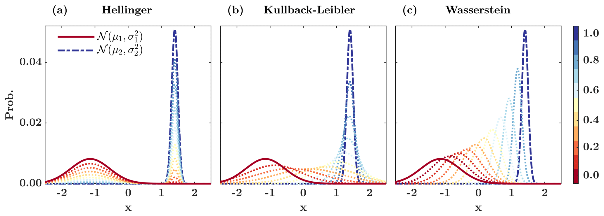
Figure 1 Interpolation between two Gaussian distributions $\mathcal{N}({\mathit{\mu }}_{\mathrm{1}},{\mathit{\sigma }}_{\mathrm{1}}^{\mathrm{2}})$ and $\mathcal{N}({\mathit{\mu }}_{\mathrm{2}},{\mathit{\sigma }}_{\mathrm{2}}^{\mathrm{2}})$, where ${\mathit{\mu }}_{\mathrm{1}}=-\mathrm{1.1},{\mathit{\mu }}_{\mathrm{2}}=\mathrm{1.4},{\mathit{\sigma }}_{\mathrm{1}}^{\mathrm{2}}=\mathrm{0.4}$, and ${\mathit{\sigma }}_{\mathrm{2}}^{\mathrm{2}}=\mathrm{0.01}$ act as a function of the interpolation or displacement parameter $\mathit{\eta }\in [\mathrm{0},\mathrm{1}]$ for the (a) Hellinger distance, (b) Kullback–Leibler divergence, and (c) 2-Wasserstein distance (Peyré and Cuturi, 2019)

As is previously noted, this metric is not limited to any Gaussian assumption. Figure 2 shows the 2-Wasserstein interpolation between a gamma and a Gaussian distribution. The results show that the Wasserstein metric penalizes the translation and mismatch between the shapes of the pdf's. It can be shown that $d_{\mathcal{W}}^{\mathrm{2}}({\mathbf{p}}_x,{\mathbf{p}}_y)=d_{\mathcal{W}}^{\mathrm{2}}({\stackrel{\mathrm{‾}}{\mathbf{p}}}_x,{\stackrel{\mathrm{‾}}{\mathbf{p}}}_y)+\parallel {\mathit{\mu }}_x-{\mathit{\mu }}_y{\parallel }_{\mathrm{2}}^{\mathrm{2}}$, where ${\stackrel{\mathrm{‾}}{\mathbf{p}}}_x$ and ${\stackrel{\mathrm{‾}}{\mathbf{p}}}_y$ are the centered zero mean probability masses, and μ_x and μ_y are the respective mean values (Peyré and Cuturi, 2019).

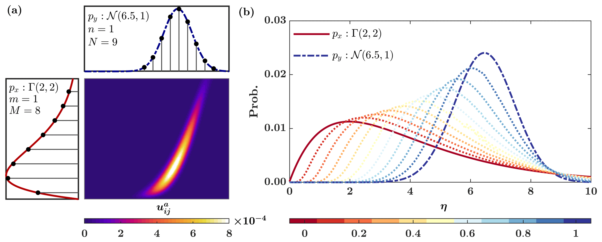
Figure 2 (a) Optimal transportation plan or the joint distribution U^a between a gamma Γ(2,2) and a Gaussian marginal distribution 𝒩(6.5,1) and (b) the 2-Wasserstein interpolation between them for different values of the displacement parameter $\mathit{\eta }\in [\mathrm{0},\mathrm{1}]$.

3 Ensemble Riemannian data assimilation

3.1 Problem formulation

First, let us recall that the weighted mean of a cloud of points ${\left\{{\mathit{x}}_i\right\}}_{i=\mathrm{1}}^M\in {\mathbb{R}}^m$ in the Euclidean space is ${\mathit{\mu }}_x={\sum }_{i=\mathrm{1}}^M{\mathit{\eta }}_i{\mathit{x}}_i$ for a given family of nonnegative weights ${\sum }_i{\mathit{\eta }}_i=\mathrm{1}$. This expected value is equivalent to solving the following variational problem:

$$\begin{array}{}\text{(4)}& {\mathit{\mu }}_x=\underset{\mathit{x}}{\mathrm{argmin}}\sum _{i=\mathrm{1}}^M{\mathit{\eta }}_i\parallel {\mathit{x}}_i-\mathit{x}{\parallel }_{\mathrm{2}}^{\mathrm{2}}.\end{array}$$

The 3D-Var problem in Eq. (2) reduces to the above barycenter problem when the model and observation error covariances are diagonal with uniform error variances across multiple dimensions of the state space. For non-diagonal error covariances, it can be shown that the weight of the background and observation are $({\mathbf{B}}^{-\mathrm{1}}+{\mathbf{H}}^{\mathrm{T}}{\mathbf{R}}^{-\mathrm{1}}\mathbf{H}{)}^{-\mathrm{1}}{\mathbf{B}}^{-\mathrm{1}}$ and $({\mathbf{B}}^{-\mathrm{1}}+{\mathbf{H}}^{\mathrm{T}}{\mathbf{R}}^{-\mathrm{1}}\mathbf{H}{)}^{-\mathrm{1}}{\mathbf{H}}^{\mathrm{T}}{\mathbf{R}}^{-\mathrm{1}}$, respectively, where H is the linear approximation of the observation operator. Therefore, the 3D-Var DA can be interpreted as a barycenter problem in the Euclidean space, where the analysis state is the weighted mean of the background state and observation.

By changing the distance metric from Euclidean to the Wasserstein (Agueh and Carlier, 2011), a Riemannian barycenter can be defined as the Fréchet mean (Fréchet, 1948) of N_p probability histograms with finite second-order moments, as follows:

$$\begin{array}{}\text{(5)}& {\mathbf{p}}_{\mathit{\eta }}=\underset{\mathbf{p}}{\mathrm{argmin}}\sum _{k=\mathrm{1}}^{N_{\mathrm{p}}}{\mathit{\eta }}_k{d}_{\mathcal{W}}^{\mathrm{2}}(\mathbf{p},{\mathbf{p}}_k).\end{array}$$

Inspired by (Feyeux et al., 2018), the EnRDA defines the probability distribution of the analysis state p(x_a)∈ℝ^M as the Fréchet barycenter over the Wasserstein space as follows:

$$\begin{array}{}\text{(6)}& \begin{array}{rl}p\left({\mathit{x}}_{\mathrm{a}}\right)& =\underset{{\mathbf{p}}_x}{\mathrm{argmin}}\\ & \left\{\mathit{\eta }{d}_{\mathcal{W}}^{\mathrm{2}}({\mathbf{p}}_x,{\mathbf{p}}_{x_b})+(\mathrm{1}-\mathit{\eta })d_{\mathcal{W}}^{\mathrm{2}}({\mathbf{p}}_x,|\det \left[{\mathcal{H}}^{\prime }\left(\mathit{x}\right)\right]\left|{\mathbf{p}}_y\right)\right\},\end{array}\end{array}$$

where the displacement parameter η>0 assigns the relative weights to the observation and background term to capture their respective geodesic distances from the true state. Here ${\mathcal{H}}^{\prime }(\cdot )$ is the Jacobian of the observation operator, assuming that $\mathcal{H}:\mathit{x}\to \mathit{y}$ is a smooth and a square (i.e., m=n) bijective map. The displacement parameter η is a hyperparameter, and its optimal value should be determined empirically using some reference data through cross-validation studies. For example, in practice, one may compute the mean squared error as a function of η, by comparing the analysis state and some ground-based observations, and use the minimum point of that function statically over a window of multiple assimilation cycles. It is also important to note that, due to the bijective assumption for the observation operator, the above formalism currently lacks the ability to propagate the information content of observed dimensions to unobserved ones. This limitation is discussed further in the Sect. 5.

The solution of the above DA formalism involves finding the optimal analysis transportation plan or the joint distribution ${\mathbf{U}}^a\in {\mathbb{R}}^{M\times N}$, using Eq. (3), that couples the background and observation marginal histograms. We use McCann's method (McCann, 1997; Peyré and Cuturi, 2019) to obtain the analysis probability histogram, as follows:

$$\begin{array}{}\text{(7)}& p\left({\mathit{x}}_{\mathrm{a}}\right)=\sum _{i=\mathrm{1}}^M\sum _{j=\mathrm{1}}^N{u}_{ij}^a{\mathit{\delta }}_{{\mathit{z}}_{ij}},\end{array}$$

where the analysis support points are ${\mathit{z}}_{ij}=\mathit{\eta }{\mathit{x}}_i+(\mathrm{1}-\mathit{\eta }){\mathit{y}}_j$. To solve Eq. (3), the widely used interior point methods (Altman and Gondzio, 1999) and Orlin's (Orlin, 1993) algorithm have a super-cubic run time with a computational complexity of O(M³log M), where M=N. Therefore, the use of the original OMT framework in EnRDA is a limitation in high-dimensional geophysical DA problems. To alleviate this computational cost, in the next Sect. 3.2, we discuss the use of entropic regularization.

To solve Eq. (6) in an ensemble setting, let us assume that, in the absence of any a priori information, the background probability distribution is initially represented by i=1…M ensemble members of the state variable x_i∈ℝ^m as $p\left({\mathit{x}}_{\mathrm{b}}\right)=\frac{\mathrm{1}}{M}{\sum }_{i=\mathrm{1}}^M{\mathit{\delta }}_{{\mathit{x}}_i}$. An a priori assumption is needed to reconstruct the observation distribution $p\left(\mathit{y}\right)={\sum }_{i=\mathrm{1}}^N{\mathbf{p}}_{y_j}{\mathit{\delta }}_{{\mathit{y}}_j}$ at j=1…N supporting points. To that end, one may choose a parametric or a nonparametric model based on the past climatological information. Here, for simplicity, we assume a zero mean Gaussian representation with covariance $\mathbf{R}\in {\mathbb{R}}^{n\times n}$ (Burgers et al., 1998) to perturb the observation at each assimilation cycle. After each cycle, the probability histogram of the analysis state p(x_a) is estimated using Eq. (7) over z_ij at M×N support points. Then p(x_a) is resampled at M points using the multinomial sampling scheme (Li et al., 2015) to initialize the next time step forecast.

3.2 Entropic regularization of EnRDA

In order to speed up the computation of the coupling, the problem in Eq. (3) can be regularized as follows (Cuturi, 2013):

$$\begin{array}{}\text{(8)}& \begin{array}{rl}{\mathbf{U}}^a& =\underset{\mathbf{U}}{\mathrm{argmin}}\langle \mathbf{C},\mathbf{U}\rangle -\mathit{\gamma }H\left(\mathbf{U}\right)\\ & \text{s.t.}\mathbf{U}\ge \mathrm{0},\mathbf{U}{\mathbf{1}}_N={\mathbf{p}}_{x_{\mathrm{b}}},{\mathbf{U}}^{\mathrm{T}}{\mathbf{1}}_M={\mathbf{p}}_y,\end{array}\end{array}$$

where γ>0 is the regularization parameter, and $H\left(\mathbf{U}\right):=\langle \mathbf{U},\log \mathbf{U}-{\mathbf{1}}_M{\mathbf{1}}_N^{\mathrm{T}}\rangle$ represents the Gibbs–Boltzmann relative entropy function. Note that the relative entropy is a concave function, and, thus its negative value is convex.

The Lagrangian function (ℒ) of Eq. (8) can be obtained by adding two dual variables or Lagrangian multipliers q∈ℝ^M and r∈ℝ^N as follows:

$$\begin{array}{}\text{(9)}& \begin{array}{rl}\mathcal{L}(\mathbf{U},\mathit{q},\mathit{r})& =\langle \mathbf{C},\mathbf{U}\rangle -\mathit{\gamma }H\left(\mathbf{U}\right)-\\ & \langle \mathit{q},\mathbf{U}{\mathbf{1}}_N-{\mathbf{p}}_{x_{\mathrm{b}}}\rangle -\langle \mathit{r},{\mathbf{U}}^{\mathrm{T}}{\mathbf{1}}_M-{\mathbf{p}}_y\rangle .\end{array}\end{array}$$

Setting the derivative of the Lagrangian function to zero, we have the following:

$$\begin{array}{}\text{(10)}& {\displaystyle \frac{\partial \mathcal{L}(\mathbf{U},\mathit{q},\mathit{r})}{\partial u_{ij}}}=c_{ij}+\mathit{\gamma }\log \left(u_{ij}\right)-q_i-r_j=\mathrm{0},\forall i,j.\end{array}$$

The entropic regularization keeps the problem in Eq. (8) strongly convex, and it can be shown (Peyré and Cuturi, 2019) that Eq. (10) leads to a unique optimal joint density with the following form:

$$\begin{array}{}\text{(11)}& {\mathbf{U}}^a=\mathrm{diag}\left(\mathit{v}\right)\mathbf{K}\mathrm{diag}\left(\mathit{w}\right),\end{array}$$

where $\mathit{v}=\exp \left(\mathit{q}\right)\oslash \left(\mathit{\gamma }{\mathbf{1}}_M\right)\in {\mathbb{R}}^M$ and $\mathit{w}=\exp \left(\mathit{r}\right)\oslash \left(\mathit{\gamma }{\mathbf{1}}_N\right)\in {\mathbb{R}}^N$ are the unknown scaling variables and $\mathbf{K}\in {\mathbb{R}}_{+}^{M\times N}$ is the Gibbs kernel with elements $k_{ij}=\exp (-\frac{c_{ij}}{\mathit{\gamma }})$, where c_ij are the elements of the cost matrix C.

From the mass conservation constraints in Eq. (8) and the scaling form of the optimal joint density in Eq. (11), we can derive the following:

$$\begin{array}{}\text{(12)}& \begin{array}{rl}& \mathrm{diag}\left(\mathit{v}\right)\mathbf{K}\mathrm{diag}\left(\mathit{w}\right){\mathbf{1}}_N={\mathbf{p}}_{x_{\mathrm{b}}}\mathrm{and}\\ & \mathrm{diag}\left(\mathit{w}\right){\mathbf{K}}^{\mathrm{T}}\mathrm{diag}\left(\mathit{v}\right){\mathbf{1}}_M={\mathbf{p}}_y.\end{array}\end{array}$$

The two unknown scaling variables v and w can then be iteratively solved using Sinkhorn's matrix scaling algorithm (Cuturi, 2013) as follows:

$$\begin{array}{}\text{(13)}& {\mathit{v}}^{l+\mathrm{1}}={\mathbf{p}}_{x_{\mathrm{b}}}\oslash \left(\mathbf{K}{\mathit{w}}^l\right)\mathrm{and}{\mathit{w}}^{l+\mathrm{1}}={\mathbf{p}}_y\oslash \left({\mathbf{K}}^{\mathrm{T}}{\mathit{v}}^l\right).\end{array}$$

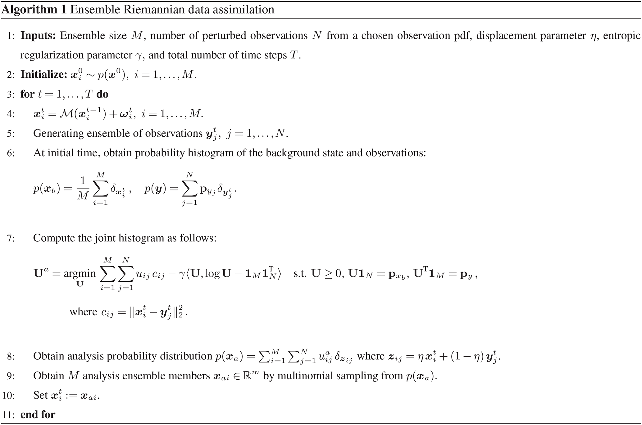
The Sinkhorn algorithm is initialized using w⁰=1_N, and since the marginal densities ${\mathbf{p}}_{x_{\mathrm{b}}}$ and p_y are not zero vectors, the Hadamard division in Eq. (13) remains valid throughout the iterations. A summary of the EnRDA implementation is demonstrated in Algorithm 1.

The entropic regularization parameter plays an important role in the characterization of the joint density; however, there exists no closed-form solution for its optimal selection. Generally speaking, increasing the value of γ will increase the convexity of the cost function and, thus, computational efficiency; however, this comes at the expense of reduced coupling between the marginal histograms, which is consistent with the second law of thermodynamics.

As an example, the effects of γ on the coupling between two Gaussian mixture models ${\mathbf{p}}_{x_{\mathrm{b}}}$ and p_y are demonstrated in Fig. 3. It can be seen that, at smaller values of γ=0.001, the probability masses of the joint distribution are sparse and lie compactly along the main diagonal – capturing a strong coupling between the background state and observations. However, as the value of γ increases, the probability masses of the joint distribution spread out – reflecting less of a degree of dependency between the marginals. It is important to note that in limiting cases, such as γ→0, the solution of Eq. (8) converges to the true optimal joint histogram, while in cases such as γ→∞, the entropy of the analysis state increases and tends to ${\mathbf{p}}_{x_{\mathrm{b}}}{\mathbf{p}}_y^{\mathrm{T}}$. The regularization parameter is dependent on the elements of the transportation cost matrix C and varies according to the experimental settings. In practice, one can begin with the value of γ set as the largest element of the cost matrix C and gradually reduce it to find the minimum value of γ that provides a stable solution.

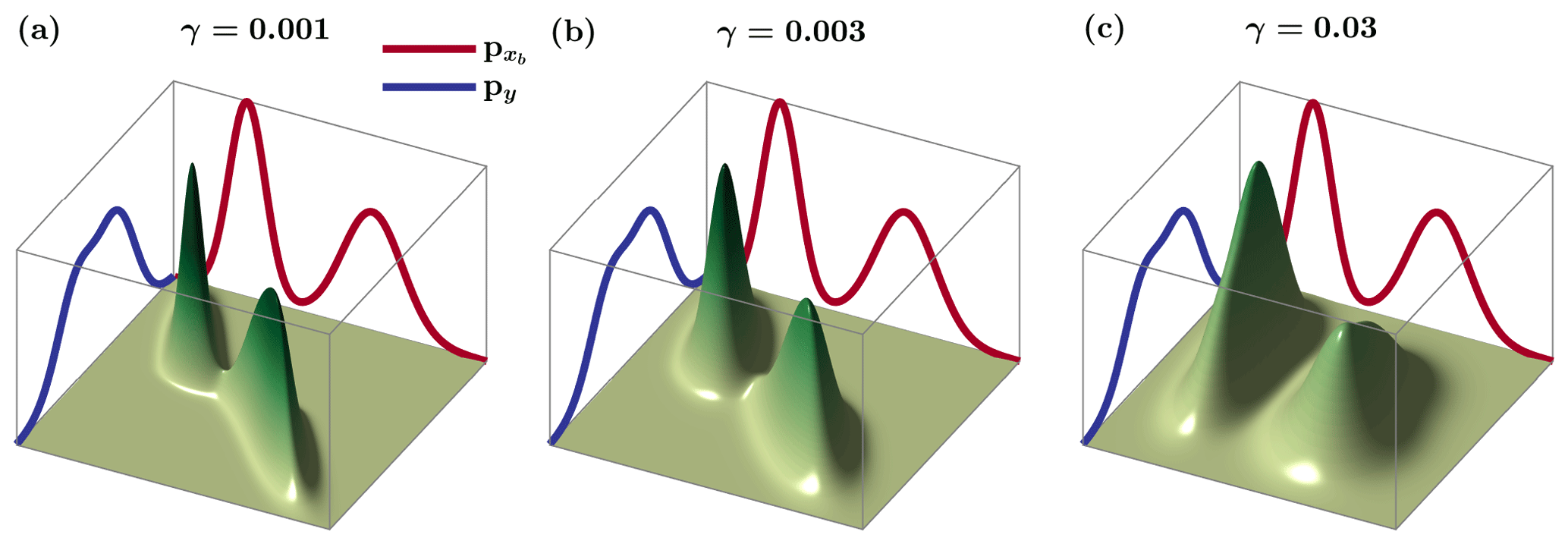
Figure 3 The effect of the entropic regularization parameter γ on the optimal joint histogram coupling two Gaussian mixture models, where ${\mathbf{p}}_{x_{\mathrm{b}}}$ is $\mathrm{0.5}\mathcal{N}(-\mathrm{12},\mathrm{0.4})+\mathrm{0.5}\mathcal{N}(-\mathrm{8},\mathrm{0.8})$ and p_y is $\mathrm{0.55}\mathcal{N}(\mathrm{5},\mathrm{4})+\mathrm{0.45}\mathcal{N}(\mathrm{9.5},\mathrm{4})$.

4 Numerical experiments and results

In order to demonstrate the performance of EnRDA and quantify its effectiveness, we focus on the linear advection–diffusion equation and the chaotic Lorenz-63 model (Lorenz, 1963). The advection–diffusion model explains a wide range of heat, mass, and momentum transport across the land, vegetation, and atmospheric continuum and has been utilized to evaluate the performance of DA methodologies (Zhang et al., 1997; Hurkmans et al., 2006; Ning et al., 2014; Ebtehaj et al., 2014; Berardi et al., 2016). Similarly, the Lorenz-63 model, as a chaotic model of atmospheric convection, has been widely used in testing the performance of DA methodologies (Miller et al., 1994; Nakano et al., 2007; Van Leeuwen, 2010; Goodliff et al., 2015; Tandeo et al., 2015; Tamang et al., 2020). Throughout, under controlled experimental settings with foreknown model and observation errors, we run the forward models under systematic errors and compare the results of EnRDA with a particle filter (PF) and an EnKF.

4.1 Advection–diffusion equation

4.1.1 State space Characterization

The advection–diffusion is a special case of the Navier–Stokes partial differential equation. In its linear form, with constant diffusivity in an incompressible fluid flow, it is expressed for a mass conserved physical quantity x(s,t) as follows:

$$\begin{array}{}\text{(14)}& {\displaystyle \frac{\partial \mathit{x}(\mathit{s},t)}{\partial t}}+\mathit{a}\odot \mathrm{\nabla }\mathit{x}(\mathit{s},t)=\mathbf{D}{\mathrm{\nabla }}^{\mathrm{2}}\mathit{x}(\mathit{s},t),\end{array}$$

where s∈ℝⁿ represents a n-dimensional spatial domain at time t. In the above expression, $\mathit{a}=(a_{\mathrm{1}},\mathrm{\dots },a_n{)}^{\mathrm{T}}\in {\mathbb{R}}^n$ is the advection velocity vector, and $\mathbf{D}=\mathrm{diag}(D_{\mathrm{1}},\mathrm{\dots },D_n)\in {\mathbb{R}}^{n\times n}$ represents the diffusivity matrix. Given the initial condition $\mathit{x}(\mathit{s},t=\mathrm{0})$, owing to its linearity, the solution at time t can be obtained by convolving the initial condition with a Kronecker delta function δ(s−a t) followed by a convolution with the fundamental Gaussian kernel $\mathcal{G}(\mathit{s},t)=\frac{\mathrm{1}}{\left(\mathrm{2}\mathit{\pi }{)}^{n/\mathrm{2}}\right|\mathbf{\Sigma }{|}^{\mathrm{1}/\mathrm{2}}}\exp \left(-\frac{\mathrm{1}}{\mathrm{2}}{\mathit{s}}^{\mathrm{T}}{\mathbf{\Sigma }}^{-\mathrm{1}}\mathit{s}\right)$, where Σ=2 D t.

4.1.2 Experimental setup and results

In this subsection, we first highlight the difference between Euclidean and Wasserstein barycenters using a 2-D advection–diffusion model and then compare the results of EnRDA with the PF and EnKF on a 1-D advection–diffusion equation.

Figure 4 shows the results of an assimilation experiment using the 2-D advection–diffusion equation where the underlying state is bimodal. This experiment is designed to demonstrate the differences between the Euclidean and Wasserstein barycenters in the presences of bias in a non-Gaussian state space. In particular, the state space is characterized over a spatial domain $s_{\mathrm{1}}=(\mathrm{0},\mathrm{10}]$ and $s_{\mathrm{2}}=(\mathrm{0},\mathrm{10}]$ with a discretization of $\mathrm{\Delta }{s}_{\mathrm{1}}=\mathrm{\Delta }{s}_{\mathrm{2}}=\mathrm{0.1}$. The advection–diffusion is considered to be an isotropic process with true model parameters set as $a_{\mathrm{1}}=a_{\mathrm{2}}=\mathrm{0.08}$ (L/T), and $D_{\mathrm{1}}=D_{\mathrm{2}}=\mathrm{0.02}$ (L²/T). The shown state variable is obtained after evolving two Kronecker delta functions $\mathit{x}(\mathit{s},t)=\mathrm{1000}\mathit{\delta }(s_{\mathrm{1}},s_{\mathrm{2}})$ and $\mathit{x}(\mathit{s},t)=\mathrm{4000}\mathit{\delta }(s_{\mathrm{1}},s_{\mathrm{2}})$ for T=0–25 and T=0–35 (T), respectively.

Figure 4 The true state x_tr, the background state x_b, and observation y (a)–(c) with systematic errors under a 2-D advection–diffusion dynamics, as well as the Euclidean (d)–(f) and the Wasserstein barycenters (g)–(i), between x_b and y for different displacement parameters η. The entropic regularization parameter is set to γ=0.003, and the black plus signs show the location of the modes for the true state.

To resemble a model with systematic errors, background state is obtained by increasing the advective velocity to 0.12 (L/T) while diffusivity is reduced to 0.01 (L²/T; Fig. 4b). Observations are not considered to have position biases; however, a systematic representative error is imposed, assuming that the sensing system has a lower resolution than the model. To that end, we evolve two Kronecker delta functions, $\mathit{x}(\mathit{s},t)=\mathrm{800}\mathit{\delta }(s_{\mathrm{1}},s_{\mathrm{2}})$ and $\mathit{x}(\mathit{s},t)=\mathrm{2400}\mathit{\delta }(s_{\mathrm{1}},s_{\mathrm{2}})$, with a mass less than the true state for same time period of T=0–25 and T=0–35 (T) and then upscale the field by a factor of 2 through box averaging (Fig. 4c).

As shown in Fig. 4g–i, the Wasserstein barycenter preserves the shape of the state variable well and gradually moves the mass towards the background state as the value of η increases, while the bias remains almost constant, and the unbiased root mean squared error (ubrmse) increases from 0.12 to 0.95. The error quality metrics are constantly below the Euclidean counterpart. As shown in Fig. 4d–f, the shape of the Euclidean barycenter for smaller values of η is not well recovered due to the position error. As η increases from 0.25 to 0.75, the Euclidean barycenter is nudged towards the background state and begins to recover the shape. The bias is reduced by more than 30 %, from 0.15 to 0.05; however, this occurs at the expense of an almost threefold increase in ubrmse, from 0.3 to 1.1. The reason for the reduction in the bias is that the positive differences between the Euclidean barycenter and the true state are compensated by their negative differences. However, ubrmse is quadratic and, thus, measures the average magnitude of the error irrespective of its signs.

For the 1-D case, the state space is characterized over a spatial domain $s\in (\mathrm{0},\mathrm{60}]$ with a discretization of Δs=0.1. The model parameters are chosen to be a=0.8 (L/T) and D=0.25 (L²/T). The initial state resembles a bimodal mixture of Gaussian distributions obtained by superposition of two Kronecker delta functions $x(s,t=\mathrm{0})=\mathrm{300}\mathit{\delta }\left(s\right)$ – evolved for time 15 and 25 (T), respectively. The ground truth of the trajectory is then obtained by evolving the initial state at a time step of Δt=0.5 over a window of T=0–30 (T) in the absence of any model error.

The observations are obtained at assimilation intervals 10Δt, assuming an identity observation operator, through corrupting the ground truth by a heteroscedastic Gaussian noise with a variance ϵ_y=5 % of the squared values of the ground truth state. We introduce both systematic and random errors in the model simulations. For the systematic error, model velocity and diffusivity coefficient are set to $a^{\prime }=\mathrm{0.12}$ (L/T) and $D^{\prime }=\mathrm{0.4}$ (L²/T), respectively. To impose the random error, a heteroscedastic Gaussian noise with variance ϵ_b=2 % is added at every Δt to model simulations. In total, 100 ensemble members are used in EnRDA, and the regularization and displacement parameters are set to γ=3 and η=0.2 through the previously outlined trial and error procedures. To obtain a robust comparison of EnRDA with PF and EnKF, each with 100 particles (ensemble members), the experiment is repeated for 50 independent simulations.

The evolution of the initial state over a time period T=0–30 (T) and the results comparing EnRDA with PF and EnKF at 5, 15, and 25 (T) are shown in Fig. 5. As demonstrated, during all time steps, EnRDA reduces the analysis uncertainty in terms of both bias and ubrmse. The shape of the entire state space is also properly preserved and remains closer to the ground truth. The EnKF performance is comparable to EnRDA during the initial time steps; however, the performance degrades and the error statistics gradually increases as the system evolves over time. Among the two traditional ensemble-based methodologies, the PF acquires the highest error statistics owing to the well-known problem of filter degeneracy (Poterjoy and Anderson, 2016), which is exacerbated by the presence of systematic errors.

Figure 5 (a) Temporal evolution of a bimodal initial state under a linear 1-D advection–diffusion equation (b)–(d) by the particle filter (PF), ensemble Kalman filter (EnKF), and ensemble Riemannian data assimilation for three time snapshots at 5, 15, and 25 (T). The bias and ubrmse of the analysis states are also reported in the legends.

We should emphasize that the presented results do not imply that EnRDA always performs better than PF and EnKF. The EnKF at the limiting case M→∞, in the absence of bias, is a minimum mean squared error estimator and attains the lowest possible posterior variance for linear systems, also referred to as the Cramér–Rao lower bound (Cramér, 1999; Rao et al., 1973). Thus, when the errors are drawn from zero mean Gaussian distributions with a linear observation operator, EnKF can outperform EnRDA in terms of the mean squared error.

4.2 Lorenz-63

4.2.1 State space characterization

The Lorenz system (Lorenz-63; Lorenz, 1963) is derived through the truncation of the Fourier series of the Rayleigh–Bénard convection model. This model can be interpreted as a simplistic local weather system only involving the effect of local shear stress and buoyancy forces. In the following, the system is expressed using coupled ordinary differential equations that describe the temporal evolution of three coordinates x, y, and z representing the rate of convective overturn, horizontal, and vertical temperature variations:

$$\begin{array}{}\text{(15)}& \begin{array}{rl}{\displaystyle \frac{\mathrm{d}x}{\mathrm{d}t}}& =-\mathit{\sigma }(x-y)\\ {\displaystyle \frac{\mathrm{d}y}{\mathrm{d}t}}& =\mathit{\rho }x-y-xz\\ {\displaystyle \frac{\mathrm{d}z}{\mathrm{d}t}}& =xy-\mathit{\beta }z,\end{array}\end{array}$$

where σ represents the Prandtl number, ρ is a normalized Rayleigh number proportional to the difference in temperature gradient through the depth of the fluid, and β denotes a horizontal wave number of the convective motion. It is well established that, for parameter values of σ=10, ρ=28, and $\mathit{\beta }=\mathrm{8}/\mathrm{3}$, the system exhibits chaotic behavior, with the phase space revolving around two unstable stationary points located at ($\sqrt{\mathit{\beta }(\mathit{\rho }-\mathrm{1})},\sqrt{\mathit{\beta }(\mathit{\rho }-\mathrm{1})},\mathit{\rho }-\mathrm{1}$) and ($-\sqrt{\mathit{\beta }(\mathit{\rho }-\mathrm{1})},-\sqrt{\mathit{\beta }(\mathit{\rho }-\mathrm{1})},\mathit{\rho }-\mathrm{1}$).

4.2.2 Experimental setup and results

Throughout the paper, we use the classic multinomial resampling for implementation of EnRDA and particle filter. Apart from the systematic error component, we utilize the standard experimental setting used in numerous DA studies (Miller et al., 1994; Furtado et al., 2008; Van Leeuwen, 2010; Amezcua et al., 2014). In order to obtain the ground truth of the model trajectory, the system is initialized at x₀=(1.508870, −1.531271, and 25.46091) and integrated with a time step of Δt=0.01 over a time period of T=0–20 (T) using the fourth-order Runge–Kutta approximation (Runge, 1895; Kutta, 1901). The observations are obtained at every assimilation interval 40Δt by assuming identity observation operator and perturbing the ground truth with Gaussian noise ${\mathit{v}}_t\sim \mathcal{N}(\mathrm{0},{\mathit{\sigma }}_{\mathrm{obs}}^{\mathrm{2}}{\mathbf{\Sigma }}_{\mathit{\rho }})$, where ${\mathit{\sigma }}_{\mathrm{obs}}^{\mathrm{2}}=\mathrm{2}$ and the correlation matrix ${\mathbf{\Sigma }}_{\mathit{\rho }}\in {\mathbb{R}}^{\mathrm{3}\times \mathrm{3}}$ is populated with 1 on the diagonal entries, 0.5 on the first sub- and super-diagonals, and 0.25 on the second sub- and super-diagonals.

In order to characterize the distribution of the background state, 100 particles (ensemble members) are used, among all DA methods, by adding to the ground truth a zero mean Gaussian noise ${\mathit{\omega }}_{\mathrm{0}}\sim \mathcal{N}(\mathrm{0},{\mathit{\sigma }}_{\mathrm{0}}^{\mathrm{2}}{\mathbf{I}}_{\mathrm{3}})$, with ${\mathit{\sigma }}_{\mathrm{0}}^{\mathrm{2}}=\mathrm{2}$ at the initial time. To introduce systematic errors, the model parameters are set to ${\mathit{\sigma }}^{\prime }=\mathrm{10.5}$, ${\mathit{\rho }}^{\prime }=\mathrm{27}$, and ${\mathit{\beta }}^{\prime }=\mathrm{10}/\mathrm{3}$. The random errors are also introduced in time by adding a Gaussian noise ${\mathit{\omega }}_t\sim \mathcal{N}(\mathrm{0},{\mathit{\sigma }}_b^{\mathrm{2}}{\mathbf{I}}_{\mathrm{3}})$ at every Δt, with ${\mathit{\sigma }}_b^{\mathrm{2}}=\mathrm{0.02}$. Throughout the paper, to draw a robust statistical inference about the error statistics, the DA experiments are repeated for 50 independent simulations. As described previously, to properly account for the effects of both bias and ubrmse, the optimal value of the displacement parameter η in EnRDA can be selected based on an offline analysis of the minimum mean squared error. However, to provide a fair comparison between EnRDA and other filtering methods, at each assimilation cycle, we set $\mathit{\eta }=\mathrm{tr}\left(\mathbf{R}\right)/\mathrm{tr}(\mathbf{R}+\mathbf{B})$ when the observation operator is an identity matrix. Note that, while the observation error covariance remains constant in time, the background error covariance is obtained from simulated ensembles and changes in time dynamically. This selection assures that the relative weights assigned to the background state and observations remain at the same order of magnitude among different methods.

Figure 6 shows the temporal evolution of the ground truth and the analysis state by the PF (first column), EnKF (second column), and EnRDA (third column) over a time period of T=0–15 (T). As is evident, the PF is well capable of capturing the ground truth when observations lie within the particle spread. However, when the observations lie far apart from the support set of particles (Fig. 6; dashed box), and the distribution of the background state and observations become disjoint, the filter becomes degenerate, and the analysis state (particle mean) deviates from the ground truth (Fig. 6g; dashed box). As a result, the bias of PF along the z dimension is markedly lower than that of the EnKF and EnRDA, while ubrmse is significantly higher, whereas EnRDA is capable of capturing the true state well – even when ensemble spread and observations are far apart from each other. Although EnKF does not suffer from the same problem of filter degeneracy as the particle filter, in earlier time steps from 2.5 to 7.5 (T), it struggles to adequately nudge the analysis state towards the ground truth when ensemble members are far from the observations due to the imposed systematic bias. EnRDA seems to be robust to the propagation of systematic errors in this region and follows the true trajectory well.

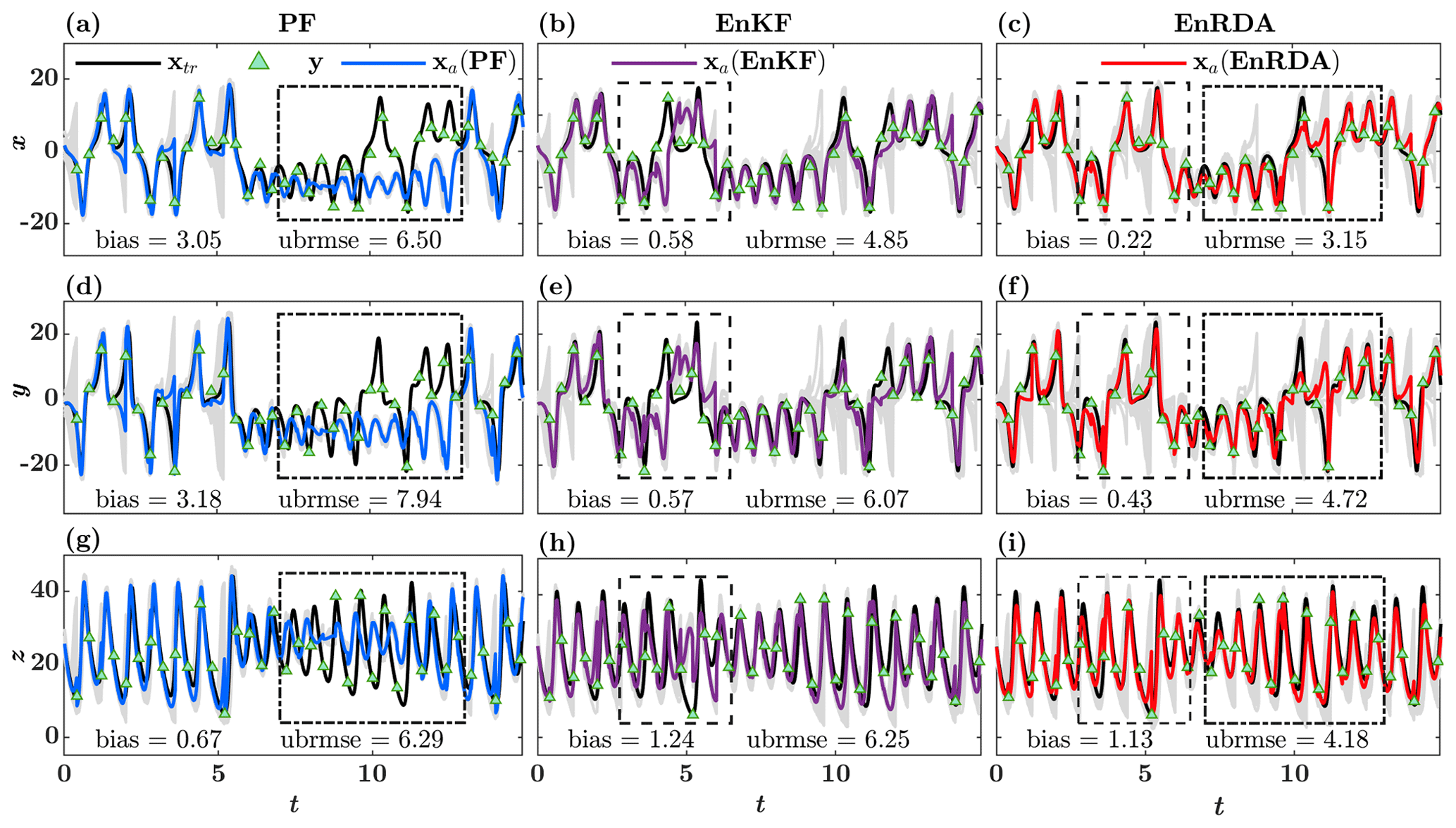
Figure 6 Temporal evolution of the true state x_tr in Lorenz-63, observations y, and the analysis state x_a for the particle filter (PF) (a, d, g), ensemble Kalman filter (EnKF) (b, e, h), and ensemble Riemannian data assimilation (EnRDA) (c, f, i), with 100 particles (ensemble members). The temporal evolution of the particles and ensemble members are shown with solid gray lines. Also shown within dashed boxes are the windows of time over which the DA methods exhibit large errors.

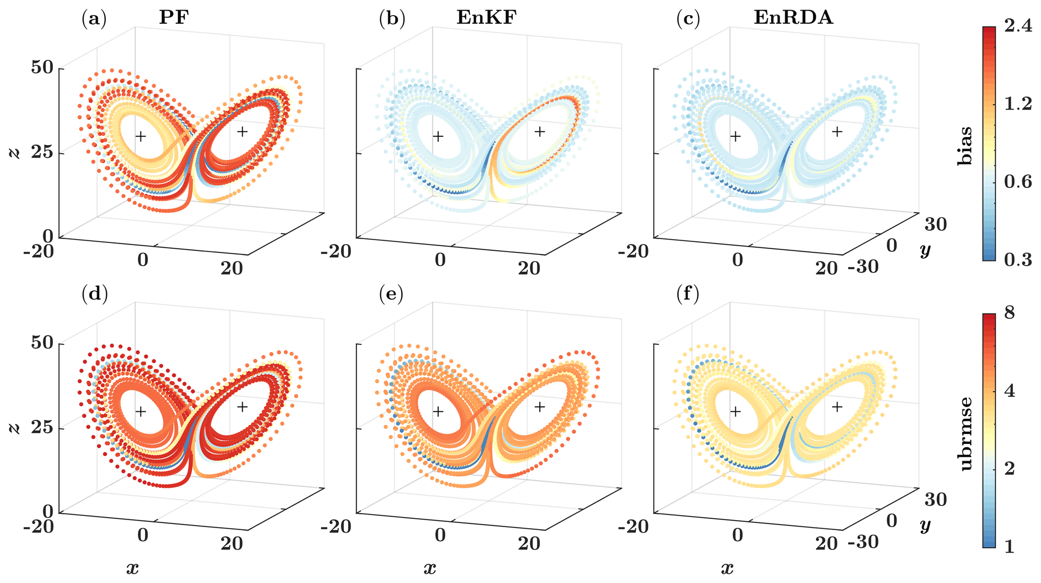
Figure 7 Temporal evolution of bias and ubrmse along three dimensions of the Lorenz-63 for the (a, d) particle filter (PF), (b, e) ensemble Kalman filter (EnKF), and (c, f) ensemble Riemannian data assimilation (EnRDA), each with 100 particles (ensemble members). The mean values are computed over 50 independent simulations.

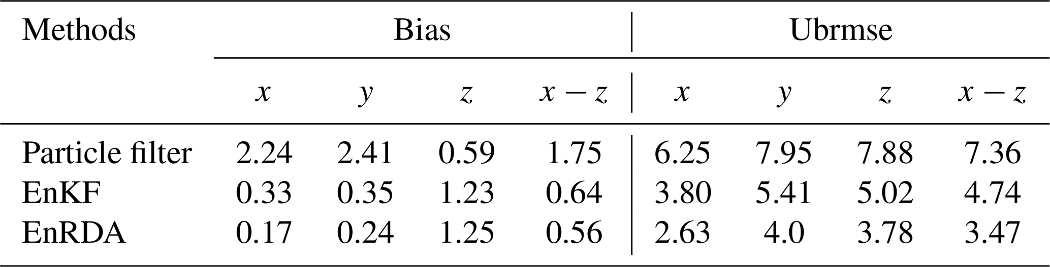
The time evolution of the bias and ubrmse for 50 independent simulations, with the same error structure, is color-coded over the phase space in Fig. 7. As shown, the error quality metrics are relatively lower for EnRDA than other DA methodologies. Nevertheless, we can see that the improvement compared to EnKF is modest. In particular, across all dimensions of the problem, the mean bias and ubrmse decreased in EnRDA by 68 (13) % and 53 (27) % compared to the particle filter (EnKF). More details about the expected values of the bias and ubrmse are reported in Table 1. We emphasize that the presented results shall be interpreted in light of the presence of systematic errors. In fact, EnRDA cannot reduce the analysis error variance beyond a minimum mean squared estimator such as EnKF in the absence of bias.

Table 1 Expected values of the bias and ubrmse for the particle filter (PF), ensemble Kalman filter (EnKF), and ensemble Riemannian data assimilation (EnRDA) for 50 independent simulations of Lorenz-63 across all problem dimensions.

5 Discussion and concluding remarks

In this study, we introduced an ensemble data assimilation (DA) methodology over a Riemannian manifold, namely ensemble Riemannian DA (EnRDA), and illustrated its performance in comparison with other ensemble-based DA techniques for dissipative and chaotic dynamics. We demonstrated that the presented methodology is capable of assimilating information in the probability domain, which is characterized by the families of distributions with finite second-order moments. The key message is that when the probability distribution of the forecast and observations exhibit a non-Gaussian structure, and their support sets are disjoint due to the presence of systematic errors; the Wasserstein metric can be leveraged to potentially extend the geophysical forecast skills. However, future research for a comprehensive comparison with existing filtering and bias correction methodologies is needed to completely characterize relative pros and cons of the proposed approach, especially when it comes to the ensemble size and optimal selection of the displacement parameter η.

We explained the role of the static regularization and displacement parameter in EnRDA and empirically examined their effects on the optimal joint histogram, coupling the background state and observations, and, consequently, on the analysis state. Nevertheless, future studies are required to characterize closed-form or heuristic expressions to expand our understating of their impacts on the forecast uncertainty dynamically. As was explained earlier, unlike the Euclidean DA methodologies that assimilate available information using different relative weights across multiple dimensions through the error covariance matrices, a scalar displacement parameter is utilized in EnRDA that interpolates uniformly between all dimensions of the problem. Future research can be devoted to developing a framework that utilizes a dynamic vector representation of the displacement parameters to effectively tackle possible the heterogeneity of uncertainty across multiple dimensions.

In its current form, EnRDA requires the observation operator to be smooth and bijective. This is a limitation when observations of all problem dimensions are not available and the propagation of observations to non-observed dimensions is desired. Extending the EnRDA methodology to include partially observed systems seems to be an important future research area. This could include performing a rough inversion for unobserved components of the system offline or extending the methodology in the direction of particle flows (Van Leeuwen et al., 2019). Another promising area is to use EnRDA only over the observed dimensions of the state space and, similar to the EnKF, use the ensemble covariance to update the unobserved part of state space through a hybrid approach. Furthermore, it is important to note that several bias correction methodologies are available that explicitly add a bias term to the control vector in variational and filtering DA techniques (Dee, 2003; Reichle and Koster, 2004; De Lannoy et al., 2007b). Future research is required to compare the performance of EnRDA with other bias correction methodologies to fully characterize its relative advantages and disadvantages.

We should mention that EnRDA is computationally expensive as it involves the estimation of the coupling through the Wasserstein distance. On a desktop machine with a 3.4 GHz CPU clock rate, it took around 1600 s to complete 50 independent simulations on Lorenz-63 for EnRDA compared to 651 (590) s for the PF (EnKF) with 100 particles (ensemble members). Since the computational cost is nonlinearly related to the problem dimension, it is expected that it grows significantly for large-scale geophysical DA and becomes a limiting factor. Furthermore, in high-dimensional geophysical problems, the computational cost of determining optimal displacement parameter η through cross-validation can be high. Although the entropic regularization works well for the presented low-dimensional problems, future research is needed to test its efficiency in high-dimensional problems. Constraining the solution of the coupling on a submanifold of probability distributions with a Gaussian mixture structure (Y. Chen et al., 2019) can also be a future research direction for lowering the computational cost. Furthermore, recent advances in approximation of the Wasserstein distance, using a combination of 1-D Radon projections and dimensionality reduction (Meng et al., 2019), can significantly reduce the computational cost to make EnRDA a viable methodology for tackling high-dimensional geophysical DA problems.

Finally, in the presented formalism, we define the analysis state distribution through an optimal coupling between forecast and observation distributions. Future lines of research can be devoted to coupling the forecast distribution with a normalized version of the likelihood function towards establishing connections with Bayesian data assimilation.