the Creative Commons Attribution 4.0 License.
the Creative Commons Attribution 4.0 License.
 | 06 May 2021
Recurrence analysis of extreme event-like data
Bedartha Goswami
Yoshito Hirata
Deniz Eroglu
Bruno Merz
Jürgen Kurths
Norbert Marwan
The identification of recurrences at various timescales in extreme event-like time series is challenging because of the rare occurrence of events which are separated by large temporal gaps. Most of the existing time series analysis techniques cannot be used to analyze an extreme event-like time series in its unaltered form. The study of the system dynamics by reconstruction of the phase space using the standard delay embedding method is not directly applicable to event-like time series as it assumes a Euclidean notion of distance between states in the phase space. The edit distance method is a novel approach that uses the point-process nature of events. We propose a modification of edit distance to analyze the dynamics of extreme event-like time series by incorporating a nonlinear function which takes into account the sparse distribution of extreme events and utilizes the physical significance of their temporal pattern. We apply the modified edit distance method to event-like data generated from point process as well as flood event series constructed from discharge data of the Mississippi River in the USA and compute their recurrence plots. From the recurrence analysis, we are able to quantify the deterministic properties of extreme event-like data. We also show that there is a significant serial dependency in the flood time series by using the random shuffle surrogate method.
- Article
(6144 KB) - Full-text XML
- BibTeX
- EndNote


One of the main challenges of society is to understand and manage natural disasters, such as earthquakes, tsunamis, and floods, which often lead to big loss of economic assets and even lives. Flooding is an important example with high societal relevance and affects more people globally than any other natural hazard. Globally, the expected annual costs of floods have been estimated to more than USD 100 billion (Desai et al., 2015). Furthermore, climate change projections point to an increasing flood risk. Direct flood damages could rise by 160 % to 240 % and human losses by 70 % to 83 % in a 1.5 ∘C warmer world (Dottori et al., 2018). Climate change has already influenced river flood magnitudes (Bloschl et al., 2019) and has been related to increases in the intensity and frequency of heavy precipitation events aggregating flash flood and river flood risk (Donat et al., 2016; Kemter et al., 2020). Natural climate variability at different timescales may lead to flood-rich and flood-poor periods (Merz et al., 2018). In addition, human interventions in river systems and catchments also heavily influence flood magnitudes and frequencies (Hall et al., 2014). Since floods can massively affect life quality of our societies, it is desirable to understand the underlying dynamics and, thus, put forward precautionary measures to avert potential disasters.
The occurrence of extreme events is not random but rather a manifestation of complex dynamics, and such events tend to have long-term correlation. Comparing data of extreme events with other non-event data using standard methods (linear/nonlinear) is problematic, because the temporal sampling differs largely (time points of events vs. continuous sampling). Furthermore, linear methods such as the Fourier transform (Bloomfield, 2004) and wavelet analysis (Percival and Walden, 2007) are often insufficient to capture the full range of dynamics occurring due to the underlying nonlinearities (Marwan, 2019). Hence, defining a principled nonlinear method is necessary for the analysis of extreme event time series, in particular when the correlation or coupling between several variables is investigated.
Out of the various approaches to study nonlinear dynamical systems (Bradley and Kantz, 2015), the reconstruction of the phase space using delay coordinates (Takens, 1981) is a widely used method that allows us to estimate dynamical invariants by constructing a topologically equivalent dynamical trajectory of the original (often high-dimensional and unknown) dynamics from the measured (scalar) time series. In the delay coordinate approach, the distance between states in the phase space plays a pivotal role in describing the underlying dynamics of a system. After reconstructing the dynamical trajectory, we can extract further information about the dynamics of a system encoded in the evolution of the distances between the trajectories, e.g., through recurrence plots (Marwan et al., 2007), correlation dimension (Grassberger and Procaccia, 1983b), Kolmogorov entropy (Grassberger and Procaccia, 1983a), or Lyapunov exponents (Wolf et al., 1985).
Although there are powerful techniques based on phase space reconstruction of a wide range of nonlinear dynamical processes, they are not directly applicable to event-like time series. Extreme events such as flood, earthquakes, or solar flares are known to have long-term correlations (Jentsch et al., 2006). However, capturing the correlations of extreme events using such methods is difficult as the phase space reconstruction and the Euclidean distance for measuring the distances of states are not suitable for event-like time series because, by definition, extreme events are small in number and are separated by large temporal gaps. In this case, it becomes necessary to define an appropriate distance measure that can help analyze the dynamics of extreme event-like time series. Event-like time series can be analyzed in their unaltered form by considering a time series of discrete events as being generated by a point process. Victor and Purpura (1997) presented a new distance metric to calculate a distance between two spike trains (binary event sequences) as a measure of similarity. Hirata and Aihara (2009) extended this idea called edit distance for converting a spike train into time series. The method has also been adopted to measure a distance between marked point processes to analyze foreign currencies (Suzuki et al., 2010) and irregularly sampled palaeoclimate data (Eroglu et al., 2016). Although the existing definition of edit distance is quite suitable for measuring similarity between event series, it introduces a bias (discussed in Sect. 3), when there are large gaps in the data as in extreme event time series. Additionally, the method depends on multiple parameters, and often it is difficult to associate a physical meaning with them. This further complicates the parameterization of the method in case of extreme events.
In this study, we propose a modification of the edit distance metric for analyzing extreme event-like time series. The proposed extension allows us to consider the shifting parameter of the edit distance metric in terms of a temporal delay which can be physically interpreted as a tolerance introduced to deal with the quasi-periodic nature of a real-world extreme event time series. We demonstrate the efficacy of the proposed modified edit distance measure by employing recurrence plots and their quantification for characterizing the dynamics of flood time series from the Mississippi River in the United States. A flood time series shows a complex time-varying behavior. Moreover, flood generation is often characterized by nonlinear catchment response to precipitation input or antecedent catchment state (Schröter et al., 2015), requiring methods able to deal with nonstationarity and nonlinearity. By using the random shuffle surrogate method, we show that there is a significant serial dependency in the flood events.
Distance measurements between two data points play an important role for many time series analysis methods, for example, in recurrence quantification analysis (RQA) (Marwan et al., 2007), estimation of the maximum Lyapunov exponent (Rosenstein et al., 1993), scale-dependent correlations (Rodó and Rodríguez-Arias, 2006), data classification (Sakoe and Chiba, 1978), and correlation dimension estimation (Grassberger, 1983). In case of regularly sampled data, the Euclidean distance is often used. However, for event-like data where big gaps between events are common, this approach is not directly applicable.
Event-like time series can be analyzed in their unaltered form by considering a time series of discrete events as being generated by a point process. Victor and Purpura (1997) presented a specific distance metric to calculate a distance between two spike trains (binary event sequences) as a measure of similarity. Hirata and Aihara (2009) extended this idea for analyzing event-like time series and named it edit distance. Ozken et al. (2015) suggested a novel interpolation scheme for irregular time series based on the edit distance, and Ozken et al. (2018) extended this approach to perform recurrence analysis for irregularly sampled data.
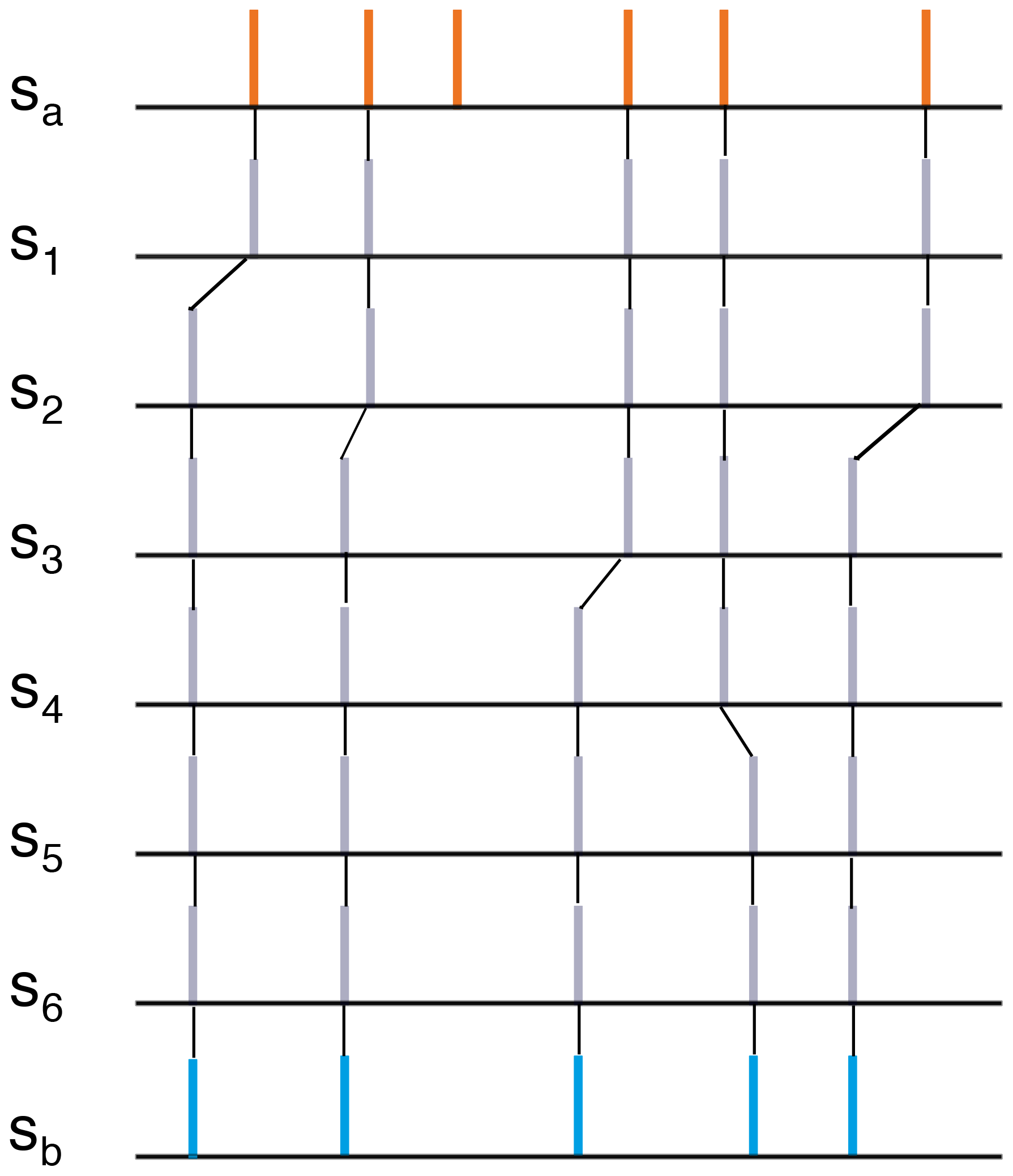
In order to apply the edit distance as a distance measure for, e.g., recurrence analysis, the whole time series is divided into small, possibly overlapping, segments (windows), which should contain some data points (Fig. 1). The aim is to determine a distance measure between every pair of segments. As a distance, we use the effort of transforming one segment into another using a certain set of operations. For this a combination of three elementary operations is required: (1) delete or (2) insert a data point and (3) shift a data point to a different point in time; each of these operations is assigned a cost. We obtain the distance measure by minimizing the total cost of this transformation. In Fig. 2, we show an illustrative example of how the elementary operations transform an arbitrary segment Sa to a segment Sb.
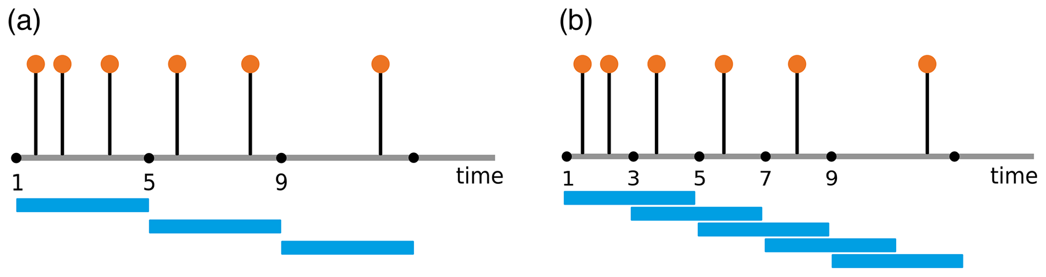
Figure 1(a) Non-overlapping windows of window size 4; (b) overlapping windows with 25 % sharing.
For the edit distance we use the sum of the costs of the three operations. The cost function is
where α and β are events in segments Sa and Sb occurring at times ta(α) and tb(β); C is the set containing all such pairs (α,β) from the two segments; I and J are the sets of indices of events in Sa and Sb; , , and are the cardinalities of I, J, and C; Λs is the cost of deletion/insertion and Λ0 the cost assigned for shifting events in time. The first summand in the cost function deals with deletion/insertion, and the second summand (the summation) deals with shifting of the pairs .
The distance D is the minimum cost needed to transform the event sequence in Sa to the event sequence in Sb:
The operation costs Λs and Λ0 are defined as
and
where M is the number of all events in the full time series. Originally, Λs was chosen as a constant value 1 (Victor and Purpura, 1997). Later, Λs was optimized in a range [0,4] (Ozken et al., 2018). The units of the parameters are (time)−1 for Λ0 and unitless for Λs.
The treatment of an event series as a point process makes the edit distance measure a good starting point for defining a distance between segments of an extreme event time series. However, the existing form of the edit distance has a linear dependency on the difference between the occurrences of events which is inappropriate for an extreme event time series, as the rare occurrence leads to large gaps between events. Also, as already mentioned, the existing method depends on a number of parameters. Therefore, we suggest a modification of the cost function to address these two concerns.
The cost of transformation between related events (e.g., events belonging to the same climatological phenomenon in a climate event series) should be lower than that between independent, unrelated events. Hence, the shifting operation should be a more likely a choice for comparison between segments if the events in each segment are related or belong to the same phenomenon. Consequently, deletion/insertion as a choice of operation for transformation tends to be associated with unrelated events.
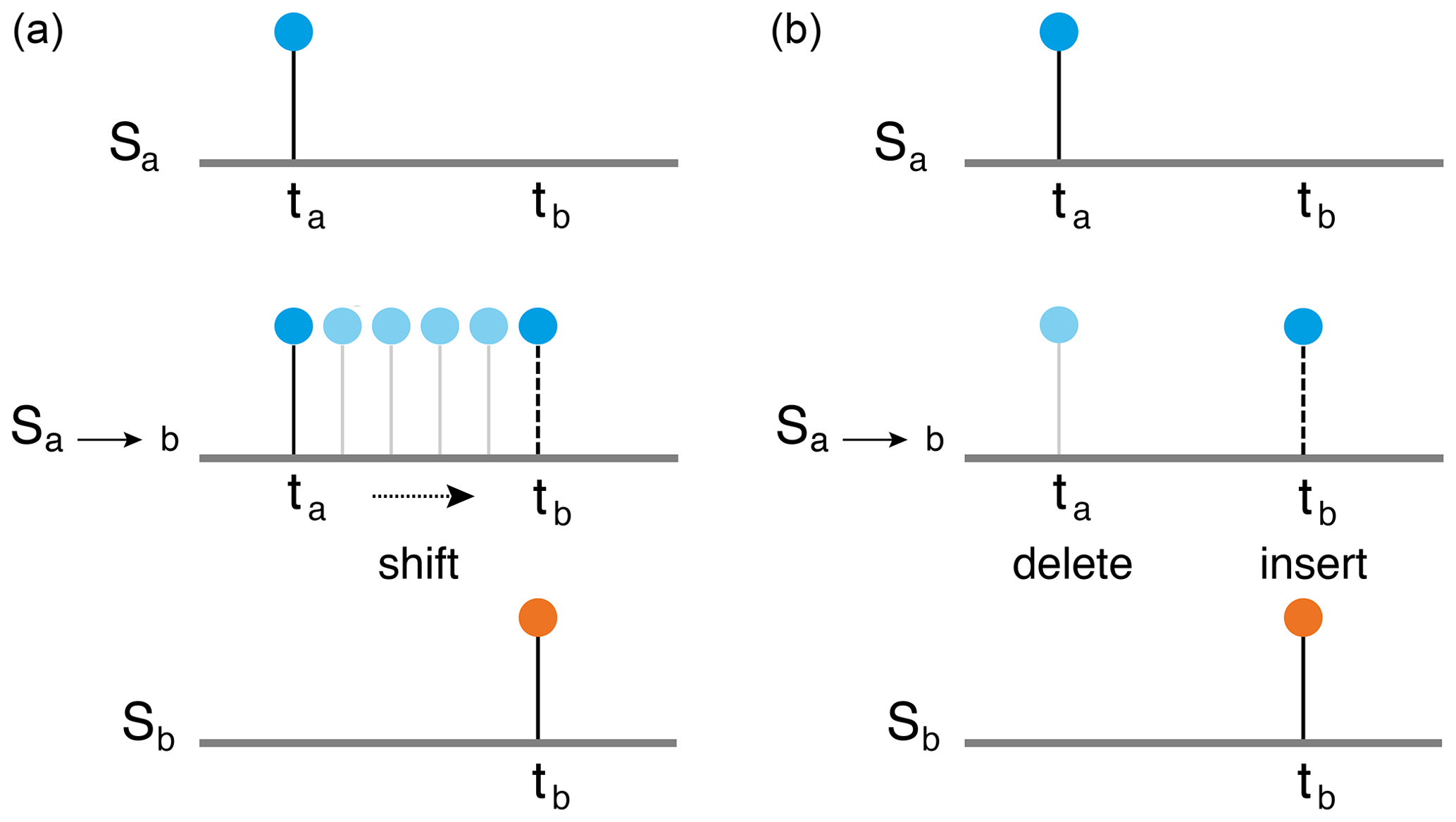
Now, we consider two event sequences Sa and Sb, where each of them has only one event at times ta and tb, respectively (Fig. 3). We want to transform segment Sa to Sb by using either deletion/insertion or shifting. The path for shifting the solitary spike has the cost Λ0Δt, where ; i.e., it grows linearly with the distance between the two events. On the other hand, the cost of deleting the event at ta from Sa and inserting it at time tb in Sa for it to resemble Sb has cost 2, as the single operation cost for deletion and insertion is each 1. So, the shifting operation will take place only as long as the time difference between both events is smaller than .
The above condition has two limiting cases which need to be considered for an unbiased choice between shifting and deletion/insertion – when the cost of shifting is too low or when it is too high. The former case arises for an extreme event time series where the number of extreme events M≪ total length of the time series, i.e., Λ0→0, Eq. (2b). This assigns a low cost for the transformation due to a biased choice of shifting over deletion/insertion for largely separated events which may be independent.
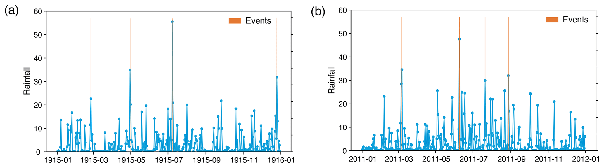
Figure 4Daily precipitation time series of the Aroostook River catchment near Masardis, Maine, in the United States for the years (a) 1915 and (b) 2011; red bars indicate extreme rainfall events (four events per year), usually occurring in spring and summer, whereas in fall extreme rainfall events usually do not occur.
The other limiting case, when the cost of shifting per unit time, Λ0, is moderately high, leads to a biased preference for the deletion/insertion operation over shifting depending on how high Λ0 is, because the cost of shifting increases linearly with the distance between two events according to the definition in Eq. (1). In this case, related events separated by a relatively small gap may be considered independent as the shifting cost may exceed the deletion/insertion cost because of higher Λ0. The following example of a real extreme event series illustrates how this biased preference can lead to erroneous results. In regions with seasonal precipitation regimes, high precipitation events are more similar to those of the same season of another year compared to other seasons. However, the exact time of occurrence of the extreme precipitation events varies from year to year; i.e., even if the events in each segment are related, there might be a certain time delay between the events (Fig. 4). Now, a linear dependency of the shifting cost on the difference between times of events, Eq. (1), does not allow us to consider small delays between potentially similar events. In addition, a not so high value of Λ0 could increase the cost of shifting for small delays higher than the cost of deletion/insertion, implying a lower similarity between the segments.
As the maximum cost for shifting is limited by the cost for deletion/insertion, we need to lower the cost of shifting to get a higher similarity between the segments for the above case. This modification is done by considering the temporal distance Δt at which the maximum cost of shifting occurs as a delay between the two events.
Selecting a certain temporal delay is relevant for climate time series, such as precipitation, or hydrological variables, like discharge, which are of an event-like nature, where the synchronization between extreme events (Malik et al., 2010, 2012; Boers et al., 2013, 2014; Ozturk et al., 2018) at different geographical locations and recurrence of extreme events for the same location are of interest.
The above discussion illustrates the importance of an appropriate choice of the cost of shifting per unit time, Λ0, based on properties of the event series, such as time series length, total number of events, and event rate. Thus it is more reasonable to optimize Λ0 as opposed to Λs. Victor and Purpura (1997) suggested generalizations of the cost assigned to finite translations, such as modifying the simple Λ0Δt to more general functions, satisfying the triangle inequality.
In view of comparing two events under a predefined delay, we suggest replacing the linear cost function for shifting, Eq. (1), by a nonlinear cost function which allows a temporal tolerance and also ensures a smooth change from the cost function for shifting to the cost for deletion/insertion (Fig. 5). We propose using the logistic function (Cramer, 2002) as the cost for shifting:
where
-
τ is the chosen time interval between events marking the transition of the function from exponential growth (for closely spaced events) to bounded exponential growth (for events separated by large time gaps) (Fig. 6a),
-
Λs is the maximum cost, and
-
k is a parameter that affects the rate of the exponential growth; in this study we choose k=1. For k=∞, the logistic function becomes a step function.
The logistic function (Eq. 3) is used for modeling the population growth in an area with limited carrying capacity.

Figure 5Linear cost function for shifting (black) and alternative, nonlinear cost function (orange).

Figure 6Variation of the cost contributed by shifting an event by Δt for different parameter values and 4.7 using (a) the logistic function with k=1 and (b) the Heaviside function.
The sigmoid nature of the logistic function is apt for representing the cost of shifting with low values for closely spaced events and which tends to saturate for events separated by a time delay greater than a certain τ.
A step function (e.g., Heaviside function) would be another choice for the cost function according to whether shifting is chosen below a certain delay and deletion/insertion is chosen above it (Fig. 6b):
where Λ0 is the cost for shifting, according to Eq. (2b), and τ is the given delay choice which decides between shifting and deletion/insertion. However, such a cost function maintains a constant value irrespective of the event spacing and switches to a different value only at the delay threshold. Therefore, the logistic function, as a smooth approximation of the step function, is a preferable choice.
The parameter optimization problem of the modified edit distance equation now becomes a problem of solving a single linear equation with two unknown variables – the coefficient related to the cost of shifting events in time and Λs. Since, in our method, we choose to optimize the former by using the logistic function, we keep Λs constant.
This constant can be absorbed in the optimization function of the first term and, therefore, the coefficient of the second term related to the cost of addition/deletion.
For a particular pair of events (α, β), we can arbitrarily set the maximum cost Λs for shifting or deletion/insertion to be 1, because it is the only free cost parameter (we have no Λk because of neglecting the amplitudes). Thus, the cost for transforming one segment to another using the modified edit distance (mED) is defined as
and the corresponding distance function to calculate the distance between two segments Sa and Sb is
This new definition of cost depends only on the parameter τ, which can be interpreted in the sense of a delay between events. Moreover, this definition holds the triangular inequality when τ satisfies a certain condition (see the Appendix for proof).
In the next section we use the modified version of edit distance to perform recurrence analysis of extreme event-like data.
A recurrence plot (RP) is a visualization of the recurrences of states of a dynamical system, capturing the essential features of the underlying dynamics into a single image. The quantification of the patterns in a RP by various measures of complexity provides further (quantitative) insights into the system's dynamics (RQA) (Marwan et al., 2007). RQA was designed to complement the nonlinearity measures such as the Lyapunov exponent, Kolmogorov entropy, information dimension, and correlation dimension (Kantz, 1994). RP-based techniques have been used in many real-world problems from various disciplines. In the field of finance, Strozzi et al. (2002) studied RQA measures for high-frequency currency exchange data. In astrophysics, Stangalini et al. (2017) applied RQA measures to detect dynamical transitions in solar activity in the last 150 years. It has also been used to classify dynamical systems (Corso et al., 2018) or to detect regime changes (Marwan et al., 2009; Eroglu et al., 2016; Trauth et al., 2019) and has many applications in Earth science (Marwan et al., 2003; Chelidze and Matcharashvili, 2007), econophysics (Kyrtsou and Vorlow, 2005; Crowley and Schultz, 2010), physiology (Webber and Zbilut, 1994; Zbilut et al., 2002; Marwan et al., 2002; Schinkel et al., 2009), and engineering (Gao et al., 2013; Oberst and Tuttle, 2018).
Consider a time series that encodes N measured states of a dynamical system on space M. A state of this system is said to be recurrent if it falls into a certain ε-neighborhood of another state. Given a distance function , for a given trajectory xi, the recurrence matrix of the system is defined as
In a RP, when , a point is plotted at (i,j); otherwise, nothing is plotted. Different classes of dynamics result in different patterns in their respective RPs (Marwan et al., 2007).
The RP contains a main diagonal line, called the line of identity (LOI), corresponding to the recurrence of a state with itself. The RP is symmetrical about the LOI when D is a metric (e.g., a symmetrical norm). We are interested in the line structures in a RP as they capture several aspects of the underlying dynamical behavior of a system. For instance, long, continuous lines parallel to the LOI denote (pseudo-)periodic behavior, whereas short, discontinuous diagonal lines are indicative of a chaotic system.
In order to incorporate mED into a RP, we divide the time series into small segments and compute the distance between these segments; the time indices are the center points of these segments. We can now define the RP in terms of the distance between the segments calculated by mED:
where ω is the number of segments and the size of the RP is ω×ω.
One of the most important measures of RQA is the determinism (DET), based on the diagonal line structures in the RP. The diagonal lines indicate those time periods where two branches of the phase space trajectory evolve parallel to each other in the phase space. The frequency distribution P(l) of the lengths of the diagonal lines is directly connected to the dynamics of the system (Marwan et al., 2007).
In our study we choose . RPs of stochastic processes mainly contain single points, resulting in low DET values, where RPs of deterministic processes contain long diagonal lines, resulting in high DET values.
In this work, we are interested in the deterministic nature of flood event time series. For this purpose, we focus on the DET measure.
We divide the time series into segments/windows. If adjacent windows overlap, we call it an overlapping sliding window, else a non-overlapping window (Fig. 1). Sliding window techniques are widely used for signal processing (Bastiaans, 1985) and activity recognition processes (Dehghani et al., 2019). The window size should be selected properly; i.e., each window should contain enough data points to be differentiable from similar movements. Consider a time series of data xi∈ℝ at times ti∈ℕ. For generalization we consider a constant sampling rate, i.e.,
Each window consists of n data points, so the window size is w=nΔT. For overlapping windows, a fraction of the data is shared between consecutive windows, denoted by as the number of data points within the overlapping range, where L=∅ signifies the non-overlapping case. The overlapping range is OL=LΔT and, in terms of percentage, %.
Because mED focuses on event-like data, finding an optimum window size is important. An inappropriate window size may lead to missing events in windows (“empty windows”) due to the sparse occurrence of events. Here we propose some criteria for choosing the optimum window size.
-
To avoid empty windows, we try to fix the number of events (n) in each window. Here we choose the window size as 1 year, as most climate phenomena such as flood events exhibit annual periodic behavior, and therefore we get a similar number of events each year.
-
In case we need to choose a larger window size to have enough data points in each window, the number of segments decreases if the windows do not overlap, which in turn reduces the dimension of the recurrence matrix. The underlying dynamical behavior of the system will not be completely captured by the resulting coarse-grained recurrence plot. Overlapping windows alleviate this problem by increasing the number of windows. In our work, we use a certain percentage of overlapping.
-
An inappropriate window size can lead to the aliasing effect (Fig. 11). As a result, different signals would be indistinguishable, and we might lose important transitions.
We apply mED first to generated data and then to real-world flood observations to understand how well our method can identify recurrences in extreme event-like time series.
6.1 Numerically generated event series using a Poisson process
The Poisson process is used as a natural model in numerous disciplines such as astronomy (Babu and Feigelson, 1996), biology (Othmer et al., 1988), ecology (Thomson, 1955), geology (Connor and Hill, 1995), or trends in flood occurrence (Swierczynski et al., 2013). It is not only used to model many real-world phenomena, but also allows for a tractable mathematical analysis.
Consider N(t) to be a stochastic counting process which represents the number of events above some specified base level in the time period (0,t). Suppose the events occur above the base level at a constant rate λ>0 (units of 1 time). So, the probability that n events occur in the time between t and t+s is given by (Ross, 1997; Loaiciga and Mariño, 1991)
A Poisson process is a set of random events whose stochastic properties do not change with time (stationary), and every event is independent of other events; i.e., the waiting time between events is memoryless (Kampen, 2007).
Here, we study three cases of numerically generated event series which are motivated by the occurrence of natural events. First, we test mED for a simple Poisson process. Each subsequent case tries to capture features of these real-world phenomena by adding an element of memory to the simple Poisson process. We compare the RPs and the structures in the RPs (by considering the RQA measure DET) derived from the standard edit distance and from the modified edit distance.
For edit distance (ED) (Eq. 1), the cost parameter for shifting is calculated according to Eq. (2a) and Λs=1, whereas Eq. (5) is used for mED. We choose the upper bound for the range of τ to be less than the mean inter-event time gap for the complete time series. The physical interpretation of this choice is that the temporal tolerance or delay in the arrival of events in a particular season (event cluster) should not only be less than the time period of the seasonal cycle, but also relatively less than the length of the season.
The selection of the threshold based on a certain percentile of the distance distribution makes the recurrence quantification more stable (Kraemer et al., 2018). Keeping in mind that this threshold should neither be too high nor too low, we chose it as the 8th to 10th percentiles of the distance distribution based on a number of trials.
It is expected that the quasi-periodic behavior of the event series will lead to high DET values. In the case of ED, the DET should be constantly high at all τ, as ED does not include the concept of time delay. On the other hand, DET computed using mED should first increase with τ and then slowly decrease.
6.1.1 Homogeneous Poisson process
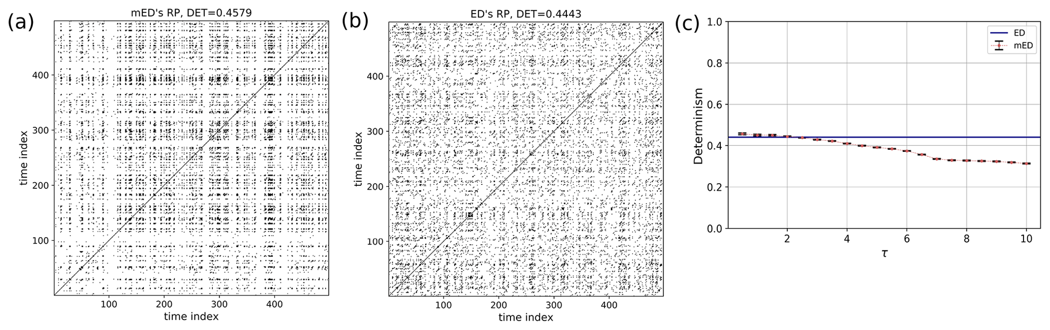
The homogeneous Poisson process models the occurrence of randomly spaced, i.e., stochastic, events in time, where the average time between the events is known. It is used to model shot noise, radioactive decay, arrival of customers at a store, earthquakes, etc. Here we construct an event series (Fig. 7a) from Eq. (9) with . The RP of a realization of such a homogeneous Poisson process is shown in Fig. 8a, b. In a stochastic process, a recurrence of a randomly selected state occurs by chance, resulting in randomly distributed points in the RP. Accordingly, DET has low values (Fig. 8c).
.

Figure 7Generated time series from a (a) homogeneous Poisson process (total length = 10 000), (b) repeating Poisson process (total length = 22 442), and (c) Poisson process with periodical forcing to mimic discharge time series (total length 0–500 with 10 000 equally spaced points); small red bars indicate the events.
6.1.2 Repeating Poisson process
We generate a small segment of a simple Poisson process and repeat the same segment after certain time gaps (Fig. 7b). Here, the Poisson process is generated for a segment of length 50 with mean rate of events . The gap between the event segments is chosen randomly in the range 105 to 115. The RP of this event series is shown in Fig. 9. Identical sequences of events result in longer diagonal lines in the RP (with lengths on the order of the event sequences), but the varying time gaps between the event chunks make the diagonal lines discontinuous, implying a quasi-periodic behavior. Quasi-periodicity is often a characteristic of an extreme event time series such as flood events. RP using ED Fig. 9b contains more short and discontinuous diagonal lines corresponding to a lower DET value. In Fig. 9c, we find a certain range where the DET value calculated using mED is higher than ED.
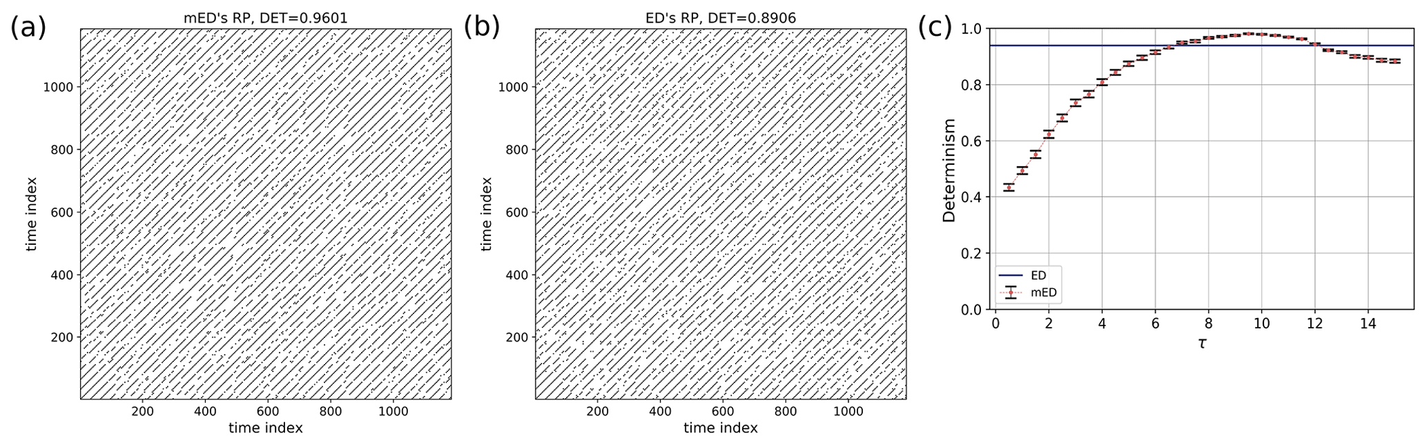
Figure 9RP of a repeating Poisson process (Fig. 7b) using (a) mED and (b) ED; (c) comparison of DET for 300 realizations using ED (blue horizontal line) and using mED for varying τ in the range 0 to 15.
6.1.3 Poisson process with periodical forcing
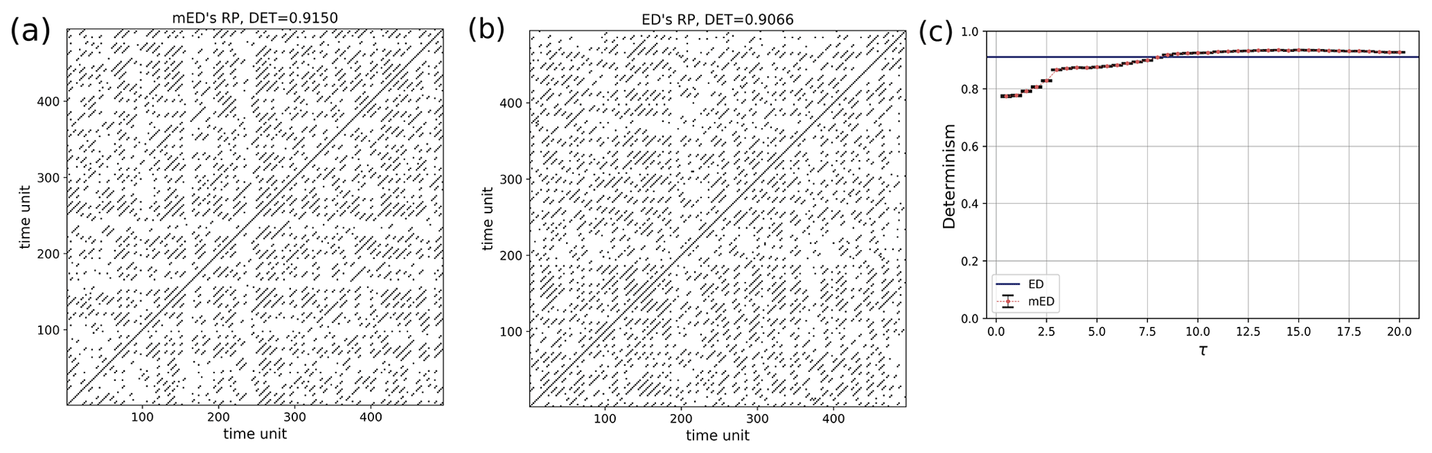
Quasi-periodicity in a time series can be expressed as a sum of harmonics with linearly independent periods. Here we construct a time series with superposition of a slow-moving signal and a fast-moving signal , whereas the events are drawn by a Poisson process (Fig. 7c). We select the extreme events by using a certain threshold and take the peak over the threshold (POT). Their occurrences and positions can be seen as the outcome of a point process (Coles, 2001). Such a time series can be used to mimic a streamflow time series which may exhibit periodic behavior on several scales (annual, seasonal, decadal, etc.). Here the window size is equal to the time period of the slow-moving signal. The RP is shown in Fig. 10. The periodic occurrences of the event chunks are visible in the RP by the line-wise accumulation of recurrence points with a constant vertical distance (which corresponds to the period). The stochastic nature of the “local” event pattern is visible by the short diagonal lines of varying lengths. As mentioned earlier, when using an improper window size, we can lose recurrence points, and a smaller number of diagonal lines occurs due to the aliasing effect (Fig. 11).
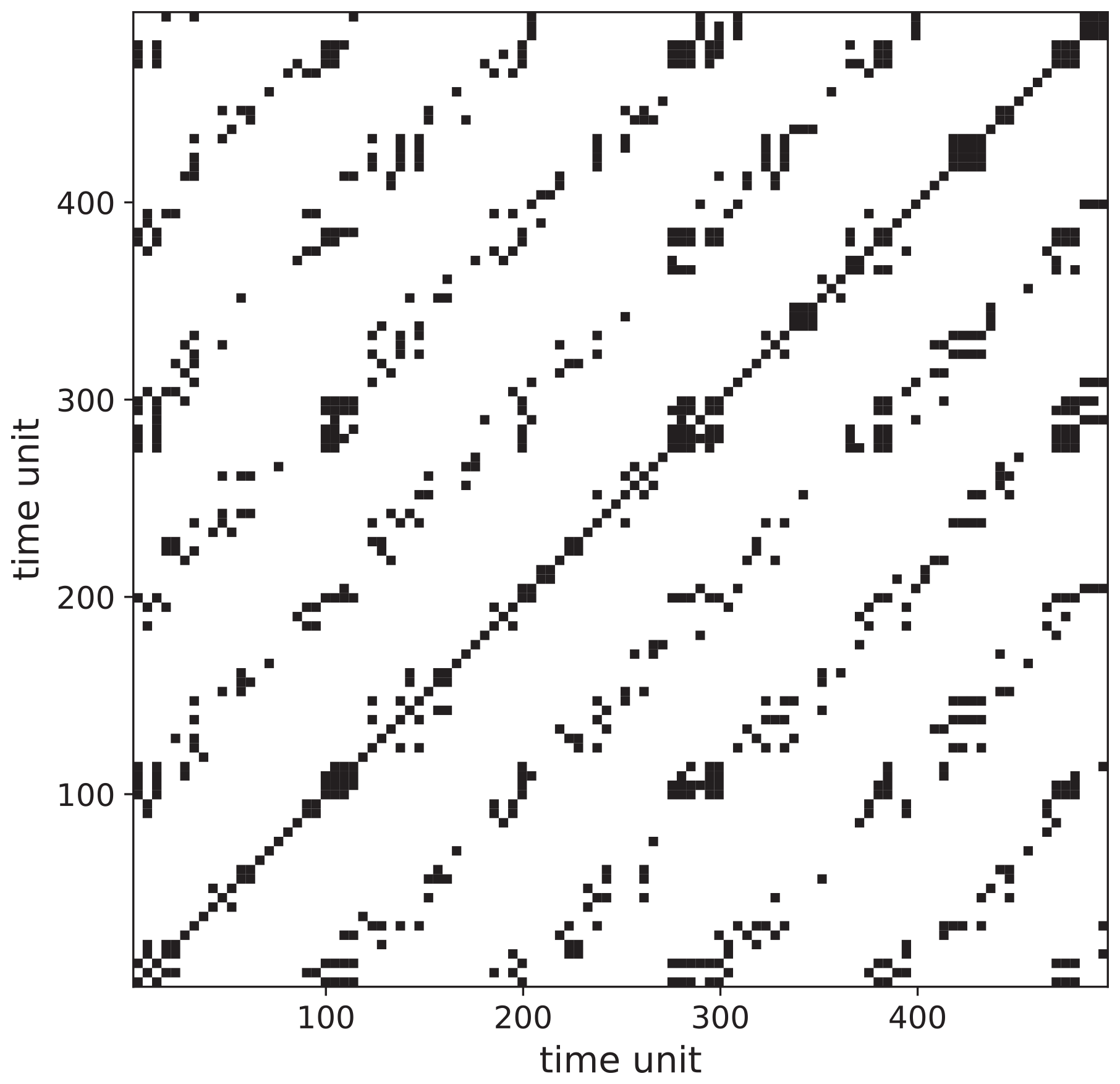
Figure 11RP of the Poisson process with periodical forcing (Fig. 7c) using mED showing the aliasing effect due to improper window size (note that this effect also occurs for the standard ED approach).
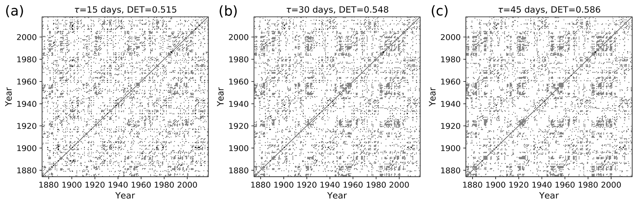
Figure 12Recurrence plot of flood events using mED, window size = 1 year, with 6 months of overlapping for delays τ= (a) 15 d, (b) 30 d, and (c) 45 d.
For a certain range of τ, DET for mED (Figs. 8, 9, and 10) is higher than the DET for ED, thus capturing the underlying periodic behavior better.
6.2 Recurrence analysis of flood events
As a case study, we apply our method to the Mississippi River, which has a rich history of flood events. Here we are motivated to study the recurring nature of flood events using recurrence plots. Recurrence plot analysis also helps to quantify the serial dependency of flood time series. Wendi et al. (2019) used RQA to study the similarity of flood events.
We use the mean daily discharge data of the Mississippi River from the Clinton, Iowa, station in the USA for the period 1874–2018. The data are obtained from the Global Runoff Data Centre (http://www.bafg.de/GRDC, last access: 15 July 2020).
In order to find the events from the time series, we follow the procedure below.
-
First, we select events above an arbitrary threshold, say the 99th percentile value of the daily discharge time series for a particular year, which gives about three to four events per year.
-
Next, if several successive days fall above the threshold forming a cluster of events, we pick only the day which has the maximum discharge value and remove the remaining events of the same cluster.
-
Then we lower the threshold by the 0.1st percentile (the threshold is lowered from the 99th to 90th) and repeat the same procedure as above until we get the desired number of events.
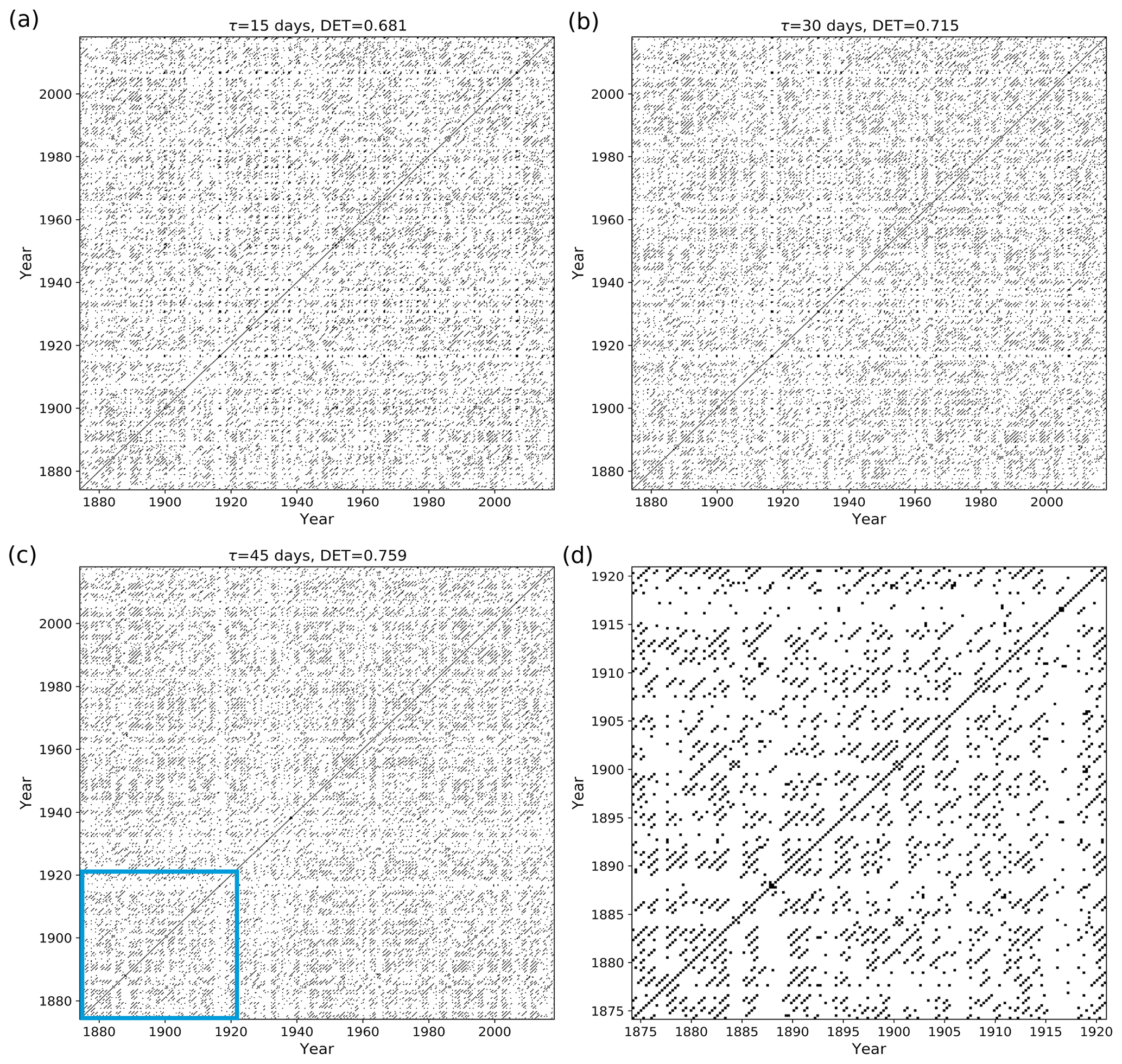
Figure 13Recurrence plot of flood events using mED, window size = 1 year, with 9 months of overlapping for delays τ= (a) 15 d, (b) 30 d, and (c) 45 d; (d) zoom-in image of the blue area of panel (c).
We apply mED for finding recurrence patterns for flood events. To this end, we choose our window size equal to the annual cycle (1 year) with 6 and 9 months of overlapping and with the cost function of delay, τ=15, 30, and 45 d. The recurrence threshold ε=8th percentile of the distance matrix. The recurrence plot of flood events is shown in Figs. 12 and 13. We also compute the recurrence plot using ED and calculate DET Fig. 14.
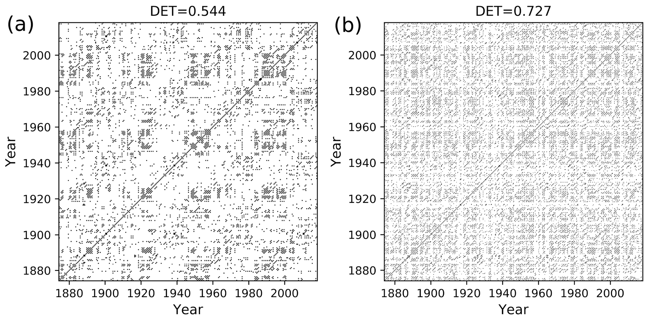
Figure 14Recurrence plot of flood events using ED, window size = 1 year, with (a) 6 months of overlapping and (b) 9 months of overlapping.
The black points in the RP (Figs. 12, 13) denote the segments which have higher similarity, and the white points imply less similarity in the occurrence of flood events. The RP of Mississippi floods shown in Fig. 13c might look similar to the RP in Fig. 8 for events generated by the Poisson process. However, the zoomed-in image of the RP of Mississippi floods, Fig 13d, is very similar to the RP in Fig. 10a for events generated by the Poisson process with periodical forcing. Diagonal structures are seen in the flood RP (Figs. 12, 13) denoting an inherent serial dependency in the data as indicated by the DET value. Serial dependency is a property by virtue of which the future depends on the past. When diagonal lines are likely to appear in a RP, the current neighbors tend to be neighbors in the near future, and thus the corresponding system is said to have serial dependence.
In order to compare the ED with the modified edit distance (mED) in the study of flood events, we compute the RP and determinism DET using both methods. For ED, there is no scope to implement a delay; we get the DET value for a constant temporal gap. In the case of mED, because of the predefined delay τ we can study the behavior at different timescales. In order to do so, we vary the parameter τ in the range from 1 to 60 d. For mED the DET values are slightly lower than ED up to τ=30 d (Fig. 15). However, after that, in the range of 30 to 60 d of τ, DET becomes higher for mED. So, for this particular time series we get more deterministic behavior for delay in the range 30 to 60 d.
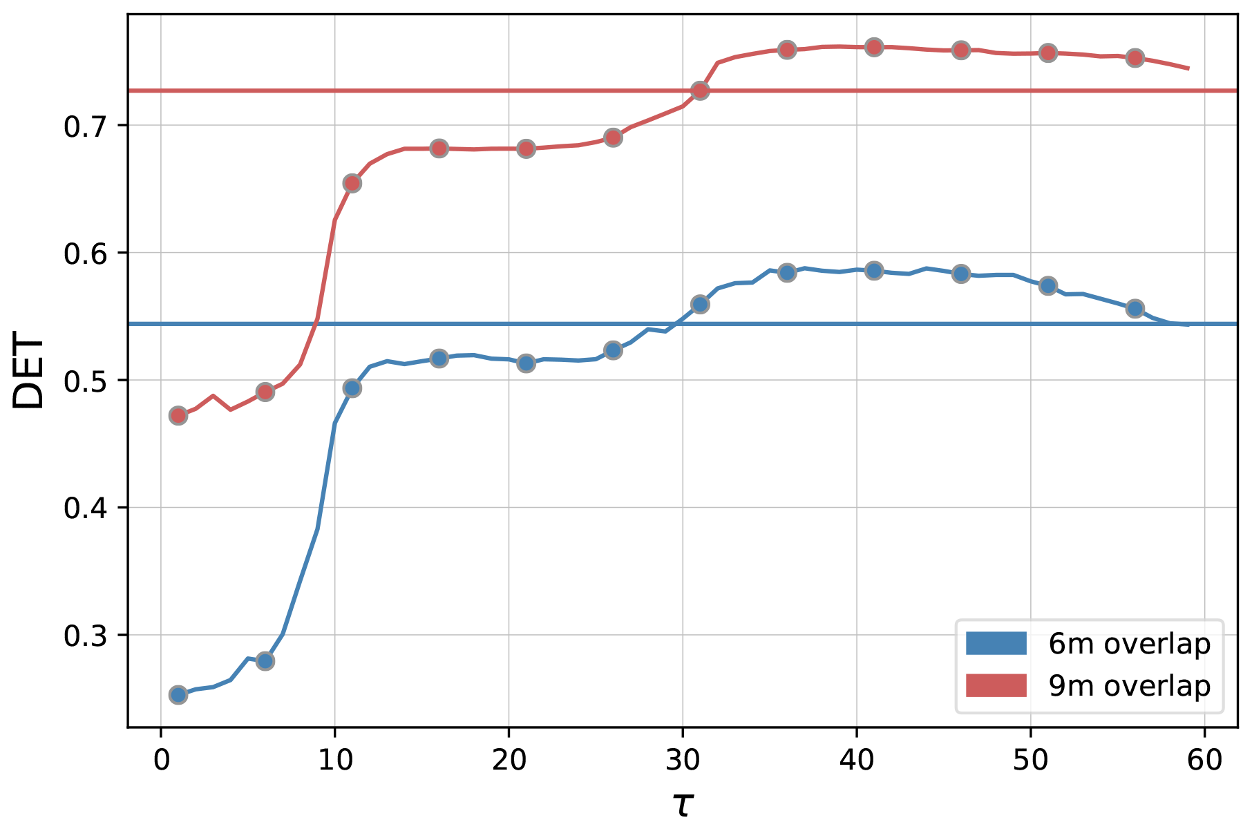
Figure 15Comparison of DET for flood events using ED (horizontal line) and using mED (curved line) for 6 months of overlapping (in blue color) and for 9 months of overlapping (in red color).
To determine the statistical significance of the RP analysis, we develop the following statistical test. We use random shuffle surrogate (Scheinkman and LeBaron, 1989) statistical testing. Suzuki et al. (2010) used this method for finding serial dependency on foreign exchange tick data by quantifying the diagonal lines in the RP (DET measure).
We first set a null hypothesis, and then we generate a set of random surrogates that preserve the null hypothesis property. After that, we compare the test statistics of the original data with the surrogate data. We can reject the null hypothesis if the test statistics obtained from the surrogate data and the original data are out of the specified range, else we cannot reject the null hypothesis.
The null hypothesis is that there is no serial dependency in the data. Thus, we expect that after each random shuffling the information will be preserved. We create each random surrogate by randomly shuffling rows and columns of a recurrence plot simultaneously. We can reject the null hypothesis if the test statistics of the original data K0 (DET value) is out of the specified range from the distribution of those surrogate datasets Ks (Theiler et al., 1992). The algorithm works as follows.
-
Calculate the distance matrix and compute the RP for a certain window size.
-
Reorder the row and columns randomly to create surrogate recurrence plots.
-
Calculate the DET of the surrogate recurrence plots.
-
Repeat steps 1–3 and get DET for 50 different surrogate RPs.
We assume the statistics obtained from the surrogates Ks is normally distributed, and we consider only one experimental dataset. The measure of “significance” as defined by Theiler et al. (1992)
follows a t distribution, the number of surrogates are n=50 with (n−1) degrees of freedom. and are the mean and standard deviation of the statistics of surrogate data. The value of ρ has to be compared to the value of the t distribution that corresponds to the 99th percentile and the mentioned degrees of freedom, i.e., . If ρ exceeds this value, the null hypothesis has to be rejected.
We measure ρ for the data generated from a homogeneous Poisson process, Eq. (9), and also for the flood event data. First, for the Poisson process the value of , so we cannot reject the null hypothesis, confirming the missing serial dependency in the homogeneous Poisson process.
For the flood event data, the distribution of the test statistics (DET) is far away from the value of the original data (Fig. 16). The ρ value for the flood event RP with 6 months of overlapping and τ=15 d is 23.80, which is much larger than 2.68. Hence, we can reject the null hypothesis at the significance level of α0=0.01, getting strong indications that there is serial dependency at a high significance level in the occurrence of flood events.
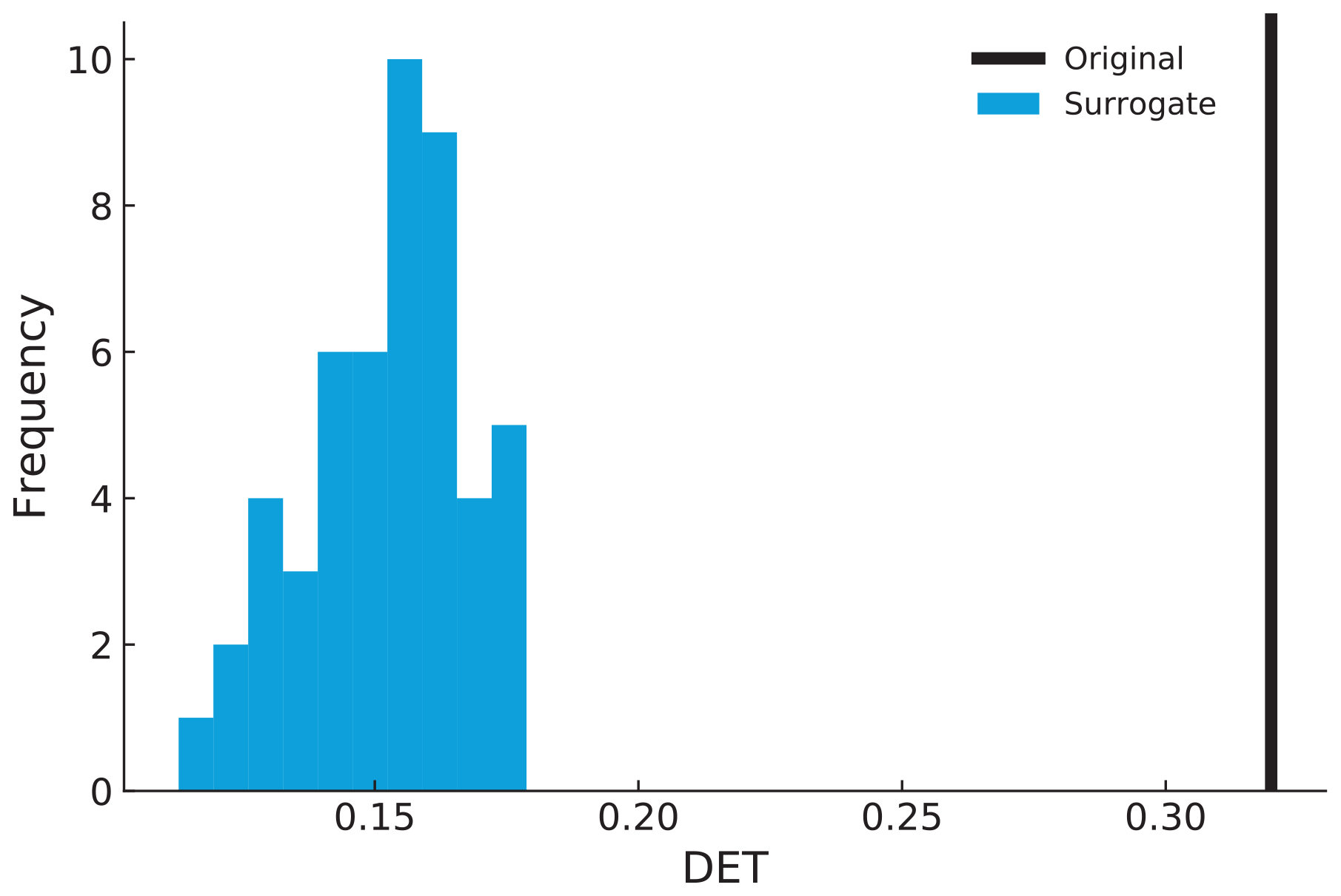
Figure 16Distribution of the DET value of surrogate data (blue) and the original DET value (black).
In this paper, we propose a distance measure for recurrence-based analysis of extreme event time series. The proposed measure is based on a modification of the edit distance measure proposed by Victor and Purpura (1997). We include the concept of time delay to incorporate the slight variation in the occurrence of recurring events of a real-world time series due to changes in seasonal patterns by replacing the linear dependency of the cost of shifting events by a nonlinear dependency using the logistic function. This is a substantial improvement over the previous definition of the edit distance as used for the TACTS algorithm proposed by Ozken et al. (2015) as the optimization of Λ0 is based on the temporal delay between events, which is of physical relevance to the study of extreme events and can be chosen according to the phenomenon being studied. The modified edit distance also reduces the number of independent parameters. We tested mED on prototypical event series generated by a point process (Poisson process). We found that for the quasi-periodic repeating Poisson process event series, the determinism of the RP computed using mED varies with temporal delay and is higher than the measured DET value of the RP computed using ED for a certain range of delay. We applied the method to study recurrences in the flood events of the Mississippi River. Our analysis revealed deterministic patterns in the occurrence of flood events from the RP. Finally, using the random shuffle surrogate method, we have shown that the data of the occurrence of flood events have a statistically significant serial dependency.
In this work, we have only considered binary extreme event time series and ignored the amplitude of events. Next, the mED measure should be further modified by including the cost due to difference in amplitude for applications in real-world time series where patterns of intensity of extremes might be of interest. Moreover, an elaborate method to optimize for a proper window size may be devised to capture recurrences of events at different timescales.
For deletions and insertions, the new definition inherits the triangle inequality for the original definition of edit distance by Victor and Purpura (1997). Thus, we can show that the new definition of the edit distance preserves the triangle inequality as a total if a shift preserves the triangle inequality. For this sake, considering the following situation is sufficient: suppose that there are three simple point processes, each of which has an event: the first point process has an event at u(u>0); the second point process has an event at ; the third point process has an event at . Therefore, the first and second point processes have an inter-event interval of s; the second and third point processes have an inter-event interval of t; and the first and third point processes have an inter-event interval of s+t.
We assume that . Then, the distance between the first and second point processes is
Likewise, the distance between the second and third point processes is
The distance between the first and third point processes is
Then, the following chain of inequalities holds.
As a result, we have
Thus, the triangle inequality holds if .
The data are obtained from the Global Runoff Data Centre (http://www.bafg.de/GRDC, BfG, 2020).
AB, BG, NM, and DE developed the theoretical formalism. AB carried out the experiment. YH verified the triangular inequality property. BM and JK closely supervised the work. AB took the lead in writing the manuscript. All the authors provided critical feedback and helped shape the research, analysis, and manuscript.
The authors declare that they have no conflict of interest.
This research has been funded by the Deutsche Forschungsgemeinschaft (DFG) within graduate research training group GRK 2043/1 “Natural risk in a changing world (NatRiskChange)” at the University of Potsdam and BMBF-funded project climXtreme. The research of Yoshito Hirata is supported by JSPS KAKENHI (JP19H00815) and the research of Deniz Eroglu is supported by a TÜBITAK (grant 118C236) Kadir Has University internal Scientific Research Grant (BAF). Bedartha Goswami is funded by the Deutsche Forschungsgemeinschaft (DFG, German Research Foundation) under Germany's Excellence Strategy – EXC number 2064/1 – project number 390727645. Abhirup Banerjee would like to thank Matthias Kemter for valuable discussions. The publication of this article was funded by the Open Access Fund of the Leibniz Association.
This research has been supported by the Deutsche Forschungsgemeinschaft (GRK 2043/1 “Natural risk in a changing world (NatRiskChange) and Germany's Excellence Strategy (EXC number 2064/1, project number 390727645)), JSPS KAKENHI (grant no. JP19H00815), and Kadir Has University internal Scientific Research Grant (BAF, grant no. 118C236).
The publication of this article was funded by the Open Access Fund of the Leibniz Association.
This paper was edited by Takemasa Miyoshi and reviewed by Carsten Brandt and Maha Mdini.
Babu, G. J. and Feigelson, E. D.: Spatial point processes in astronomy, J. Stat. Plan. Infer., 50, 311–326, https://doi.org/10.1016/0378-3758(95)00060-7, 1996. a
Bastiaans, M.: On the sliding-window representation in digital signal processing, IEEE T. Acoust. Speech, 33, 868–873, 1985. a
Bloomfield, P.: Fourier Analysis of Time Series: An Introduction, Wiley Series in Probability and Statistics, Wiley, available at: https://books.google.de/books?id=zQsupRg5rrAC (last access: 7 April 2020), 2004. a
Bloschl, G., Hall, J., Kjeldsen, T., and Macdonald, N.: Changing climate both increases and decreases European river floods, Nature, 573, 108–111, https://doi.org/10.1038/s41586-019-1495-6, 2019. a
Boers, N., Bookhagen, B., Marwan, N., Kurths, J., and Marengo, J.: Complex networks identify spatial patterns of extreme rainfall events of the South American Monsoon System, Geophys. Res. Lett., 40, 4386–4392, https://doi.org/10.1002/grl.50681, 2013. a
Boers, N., Rheinwalt, A., Bookhagen, B., Barbosa, H. M. J., Marwan, N., Marengo, J., and Kurths, J.: The South American rainfall dipole: A complex network analysis of extreme events, Geophys. Res. Lett., 41, 7397–7405, https://doi.org/10.1002/2014GL061829, 2014. a
Bradley, E. and Kantz, H.: Nonlinear time-series analysis revisited, Chaos, 25, 097610, https://doi.org/10.1063/1.4917289, 2015. a
Bundesanstalt für Gewässerkunde (BfG): Global Runoff Data Centre, available at: http://www.bafg.de/GRDC, last access: 15 July 2020. a
Chelidze, T. and Matcharashvili, T.: Complexity of seismic process; measuring and applications – A review, Tectonophysics, 431, 49–60, https://doi.org/10.1016/j.tecto.2006.05.029, 2007. a
Coles, S.: An introduction to statistical modeling of extreme values, Springer Series in Statistics, Springer-Verlag, London, UK, 2001. a
Connor, C. B. and Hill, B. E.: Three nonhomogeneous Poisson models for the probability of basaltic volcanism: Application to the Yucca Mountain region, Nevada, J. Geophys. Res.-Sol. Ea., 100, 10107–10125, https://doi.org/10.1029/95JB01055, 1995. a
Corso, G., Prado, T. D. L., Lima, G. Z. D. S., Kurths, J., and Lopes, S. R.: Quantifying entropy using recurrence matrix microstates, Chaos, 28, 083108, https://doi.org/10.1063/1.5042026, 2018. a
Cramer, J.: The Origins of Logistic Regression, Tinbergen Institute Discussion Papers, 02-119, available at: https://ideas.repec.org/p/tin/wpaper/20020119.html (last access: 15 April 2020), 2002. a
Crowley, P. M. and Schultz, A.: A new approach to analyzing convergence and synchronicity in growth and business cycles: cross recurrence plots and quantification analysis, Bank of Finland Research – Discussion Papers, 16, 3–51, available at: https://ideas.repec.org/p/pra/mprapa/23728.html (last access: 5 May 2020), 2010. a
Dehghani, A., Sarbishei, O., Glatard, T., and Shihab, E.: A quantitative comparison of overlapping and non-overlapping sliding windows for human activity recognition using inertial sensors, Sensors (Switzerland), 19, 10–12, https://doi.org/10.3390/s19225026, 2019. a
Desai, B., Maskrey, A., Peduzzi, P., De Bono, A., and Herold, C.: Making Development Sustainable: The Future of Disaster Risk Management, Global Assessment Report on Disaster Risk Reduction, available at: https://archive-ouverte.unige.ch/unige:78299 (last access: 21 February 2020), 2015. a
Donat, M., Lowry, A., Alexander, L., O'Gorman, P., and Maher, N.: More extreme precipitation in the world’s dry and wet regions, Nat. Clim. Change, 6, 508–513, https://doi.org/10.1038/nclimate2941, 2016. a
Dottori, F., Szewczyk, W., Ciscar, J., Zhao, F., Alfieri, L., Hirabayashi, Y., Bianchi, A., Mongelli, I., Frieler, K., Betts, R., and Feyen, L.: Increased human and economic losses from river flooding with anthropogenic warming, Nat. Clim. Change, 8, 781–786, https://doi.org/10.1038/s41558-018-0257-z, 2018. a
Eroglu, D., McRobie, F. H., Ozken, I., Stemler, T., Wyrwoll, K.-H., Breitenbach, S. F. M., Marwan, N., and Kurths, J.: See-saw relationship of the Holocene East Asian-Australian summer monsoon, Nat. Commun., 7, 12929, https://doi.org/10.1038/ncomms12929, 2016. a, b
Gao, Z., Zhang, X., Jin, N., Donner, R. V., Marwan, N., and Kurths, J.: Recurrence networks from multivariate signals for uncovering dynamic transitions of horizontal oil-water stratified flows, Europhys. Lett., 103, 50004, https://doi.org/10.1209/0295-5075/103/50004, 2013. a
Grassberger, P.: Generalized Dimensions of Strange Attractors, Phys. Lett. A, 97, 227–230, https://doi.org/10.1016/0375-9601(83)90753-3, 1983. a
Grassberger, P. and Procaccia, I.: Estimation of the Kolmogorov entropy from a chaotic signal, Phys. Rev. A, 9, 2591–2593, https://doi.org/10.1103/PhysRevA.28.2591, 1983a. a
Grassberger, P. and Procaccia, I.: Characterization of strange attractors, Phys. Rev. Lett., 50, 346–349, https://doi.org/10.1103/PhysRevLett.50.346, 1983b. a
Hall, J., Arheimer, B., Borga, M., Brázdil, R., Claps, P., Kiss, A., Kjeldsen, T. R., Kriaučiūnienė, J., Kundzewicz, Z. W., Lang, M., Llasat, M. C., Macdonald, N., McIntyre, N., Mediero, L., Merz, B., Merz, R., Molnar, P., Montanari, A., Neuhold, C., Parajka, J., Perdigão, R. A. P., Plavcová, L., Rogger, M., Salinas, J. L., Sauquet, E., Schär, C., Szolgay, J., Viglione, A., and Blöschl, G.: Understanding flood regime changes in Europe: a state-of-the-art assessment, Hydrol. Earth Syst. Sci., 18, 2735–2772, https://doi.org/10.5194/hess-18-2735-2014, 2014. a
Hirata, Y. and Aihara, K.: Representing spike trains using constant sampling intervals, J. Neurosci. Meth., 183, 277–286, https://doi.org/10.1016/j.jneumeth.2009.06.030, 2009. a, b
Jentsch, V., Kantz, H., and Albeverio, S.: Extreme Events: Magic, Mysteries, and Challenges, Springer Berlin Heidelberg, Berlin, Heidelberg, 1–18, https://doi.org/10.1007/3-540-28611-X_1, 2006. a
Kampen, N. V.: Stochastic processes in physics and chemistry, 3rd edn., North-Holland Personal Library, Elsevier, Amsterdam, the Netherlands, https://doi.org/10.1016/B978-044452965-7/50005-2, 2007. a
Kantz, H.: A robust method to estimate the maximal Lyapunov exponent of a time series, Phys. Lett. A, 185, 77–87, https://doi.org/10.1016/0375-9601(94)90991-1, 1994. a
Kemter, M., Merz, B., Marwan, N., Vorogushyn, S., and Blöschl, G.: Joint Trends in Flood Magnitudes and Spatial Extents Across Europe, Geophys. Res. Lett., 47, e2020GL087464, https://doi.org/10.1029/2020GL087464, 2020. a
Kraemer, K. H., Donner, R. V., Heitzig, J., and Marwan, N.: Recurrence threshold selection for obtaining robust recurrence characteristics in different embedding dimensions, Chaos, 28, 085720, https://doi.org/10.1063/1.5024914, 2018. a
Kyrtsou, C. and Vorlow, C. E.: Complex Dynamics in Macroeconomics: A Novel Approach, in: New Trends in Macroeconomics, edited by: Diebolt, C. and Kyrtsou, C., 223–238, https://doi.org/10.1007/3-540-28556-3_11, 2005. a
Loaiciga, H. A. and Mariño, M. A.: Recurrence Interval of Geophysical Events, J. Water Res. Pl., 117, 367–382, https://doi.org/10.1061/(ASCE)0733-9496(1991)117:3(367), 1991. a
Malik, N., Marwan, N., and Kurths, J.: Spatial structures and directionalities in Monsoonal precipitation over South Asia, Nonlin. Processes Geophys., 17, 371–381, https://doi.org/10.5194/npg-17-371-2010, 2010. a
Malik, N., Bookhagen, B., Marwan, N., and Kurths, J.: Analysis of spatial and temporal extreme monsoonal rainfall over South Asia using complex networks, Clim. Dynam., 39, 971–987, https://doi.org/10.1007/s00382-011-1156-4, 2012. a
Marwan, N.: Recurrence Plot Techniques for the Investigation of Recurring Phenomena in the System Earth, University of Potsdam, https://doi.org/10.25932/publishup-44197, 2019. a
Marwan, N., Wessel, N., Meyerfeldt, U., Schirdewan, A., and Kurths, J.: Recurrence Plot Based Measures of Complexity and its Application to Heart Rate Variability Data, Physical Review E, 66, 026702, https://doi.org/10.1103/PhysRevE.66.026702, 2002. a
Marwan, N., Trauth, M. H., Vuille, M., and Kurths, J.: Comparing modern and Pleistocene ENSO-like influences in NW Argentina using nonlinear time series analysis methods, Clim. Dynam., 21, 317–326, https://doi.org/10.1007/s00382-003-0335-3, 2003. a
Marwan, N., Romano, M. C., Thiel, M., and Kurths, J.: Recurrence Plots for the Analysis of Complex Systems, Phys. Rep., 438, 237–329, https://doi.org/10.1016/j.physrep.2006.11.001, 2007. a, b, c, d, e
Marwan, N., Donges, J. F., Zou, Y., Donner, R. V., and Kurths, J.: Complex network approach for recurrence analysis of time series, Phys. Lett. A, 373, 4246–4254, https://doi.org/10.1016/j.physleta.2009.09.042, 2009. a
Merz, B., Dung, N. V., Apel, H., Gerlitz, L., Schröter, K., Steirou, E., and Vorogushyn, S.: Spatial coherence of flood-rich and flood-poor periods across Germany, J. Hydrol., 559, 813–826, https://doi.org/10.1016/j.jhydrol.2018.02.082, 2018. a
Oberst, S. and Tuttle, S.: Nonlinear dynamics of thin-walled elastic structures for applications in space, Mech. Syst. Signal Pr., 110, 469–484, https://doi.org/10.1016/j.ymssp.2018.03.021, 2018. a
Othmer, H., Dunbar, S., and Alt, W.: Models of dispersal in biological systems, J. Math. Biol., 26, 263–298, https://doi.org/10.1007/bf00277392, 1988. a
Ozken, I., Eroglu, D., Stemler, T., Marwan, N., Bagci, G. B., and Kurths, J.: Transformation-cost time-series method for analyzing irregularly sampled data, Phys. Rev. E, 91, 062911, https://doi.org/10.1103/PhysRevE.91.062911, 2015. a, b
Ozken, I., Eroglu, D., Breitenbach, S. F. M., Marwan, N., Tan, L., Tirnakli, U., and Kurths, J.: Recurrence plot analysis of irregularly sampled data, Phys. Rev. E, 98, 052215, https://doi.org/10.1103/PhysRevE.98.052215, 2018. a, b
Ozturk, U., Marwan, N., Korup, O., Saito, H., Agarwal, A., Grossman, M. J., Zaiki, M., and Kurths, J.: Complex networks for tracking extreme rainfall during typhoons, Chaos, 28, 075301, https://doi.org/10.1063/1.5004480, 2018. a
Percival, D. B. and Walden, A. T.: Wavelet methods for time series analysis, Cambridge Univ. Press, Cambridge, available at: http://www.worldcat.org/title/wavelet-methods-for-time-series-analysis/oclc/254371438 (last access: 3 May 2020), 2007. a
Rodó, X. and Rodríguez-Arias, M.-A.: A new method to detect transitory signatures and local time/space variability structures in the climate system: the scale-dependent correlation analysis, Clim. Dynam., 27, 441–458, https://doi.org/10.1007/s00382-005-0106-4, 2006. a
Rosenstein, M. T., Collins, J. J., and De Luca, C. J.: A practical method for calculating largest Lyapunov exponents from small data sets, Physica D, 65, 117–134, https://doi.org/10.1016/0167-2789(93)90009-P, 1993. a
Ross, S. M.: Introduction to Probability Models, 6th edn., Academic Press, San Diego, CA, USA, 1997. a
Sakoe, H. and Chiba, S.: Dynamic Programming Algorithm Optimization for Spoken Word Recognition, IEEE T. Acoust. Speech, ASSP-26, 43–49, 1978. a
Scheinkman, J. A. and LeBaron, B.: Nonlinear dynamics and GNP data, in: Economic complexity: chaos, sunspots, bubbles, and nonlinearity, Cambridge University Press, Cambridge, UK, 213–227, 1989. a
Schinkel, S., Marwan, N., Dimigen, O., and Kurths, J.: Confidence bounds of recurrence-based complexity measures, Phys. Lett. A, 373, 2245–2250, https://doi.org/10.1016/j.physleta.2009.04.045, 2009. a
Schröter, K., Kunz, M., Elmer, F., Mühr, B., and Merz, B.: What made the June 2013 flood in Germany an exceptional event? A hydro-meteorological evaluation, Hydrol. Earth Syst. Sci., 19, 309–327, https://doi.org/10.5194/hess-19-309-2015, 2015. a
Stangalini, M., Ermolli, I., Consolini, G., and Giorgi, F.: Recurrence quantification analysis of two solar cycle indices, J. Space Weather Spac., 7, 1–13, https://doi.org/10.1051/swsc/2017004, 2017. a
Strozzi, F., Zaldívar, J.-M., and Zbilut, J. P.: Application of nonlinear time series analysis techniques to high-frequency currency exchange data, Physica A, 312, 520–538, https://doi.org/10.1016/S0378-4371(02)00846-4, 2002. a
Suzuki, S., Hirata, Y., and Aihara, K.: Definition of distance for marked point process data and its application to recurrence plot-based analysis of exchange tick data of foreign currencies, Int. J. Bifurcat. Chaos, 20, 3699–3708, https://doi.org/10.1142/S0218127410027970, 2010. a, b
Swierczynski, T., Lauterbach, S., Dulski, P., Delgado, J., Merz, B., and Brauer, A.: Mid- to late Holocene flood frequency changes in the northeastern Alps as recorded in varved sediments of Lake Mondsee (Upper Austria), Quaternary Sci. Rev., 80, 78–90, https://doi.org/10.1016/j.quascirev.2013.08.018, 2013. a
Takens, F.: Detecting Strange Attractors in Turbulence, in: Dynamical Systems and Turbulence, edited by: Rand, D. and Young, L.-S., vol. 898 of Lecture Notes in Mathematics, Springer, Berlin, Germany, 366–381, 1981. a
Theiler, J., Eubank, S., Longtin, A., Galdrikian, B., and Farmer, B.: Testing for nonlinearity in time series: the method of surrogate data, Physica D, 58, 77–94, https://doi.org/10.1016/0167-2789(92)90102-S, 1992. a, b
Thomson, H. R.: Spatial Point Processes, With Applications To Ecology, Biometrika, 42, 102–115, https://doi.org/10.1093/biomet/42.1-2.102, 1955. a
Trauth, M. H., Asrat, A., Duesing, W., Foerster, V., Kraemer, K. H., Marwan, N., Maslin, M. A., and Schaebitz, F.: Classifying past climate change in the Chew Bahir basin, southern Ethiopia, using recurrence quantification analysis, Clim. Dynam., 53, 2557–2572, https://doi.org/10.1007/s00382-019-04641-3, 2019. a
Victor, J. D. and Purpura, K. P.: Metric-space analysis of spike trains: theory, algorithms and application, Network-Comp. Neural, 8, 127–164, 1997. a, b, c, d, e, f
Webber, Jr., C. L. and Zbilut, J. P.: Dynamical assessment of physiological systems and states using recurrence plot strategies, J. Appl. Physiol., 76, 965–973, 1994. a
Wendi, D., Merz, B., and Marwan, N.: Assessing Hydrograph Similarity and Rare Runoff Dynamics by Cross Recurrence Plots, Water Resour. Res., 55, 4704–4726, https://doi.org/10.1029/2018WR024111, 2019. a
Wolf, A., Swift, J. B., Swinney, H. L., and Vastano, J. A.: Determining Lyapunov Exponents from a Time Series, Physica D, 16, 285–317, https://doi.org/10.1016/0167-2789(85)90011-9, 1985. a
Zbilut, J. P., Thomasson, N., and Webber, Jr., C. L.: Recurrence quantification analysis as a tool for nonlinear exploration of nonstationary cardiac signals, Med. Eng. Phys., 24, 53–60, https://doi.org/10.1016/S1350-4533(01)00112-6, 2002. a
- Abstract
- Introduction
- Edit distance for event-like time series
- Modified edit distance
- Recurrence plots
- Choice of window size
- Applications of modified edit distance
- Conclusion
- Appendix A
- Data availability
- Author contributions
- Competing interests
- Acknowledgements
- Financial support
- Review statement
- References