Anthropocene climate bifurcation

This article presents the results of a bifurcation analysis of a simple energy balance model (EBM) for the future climate of the Earth. The main focus is on the following question: can the nonlinear processes intrinsic to atmospheric physics, including natural positive feedback mechanisms, cause a mathematical bifurcation of the climate state, as a consequence of continued anthropogenic forcing by rising greenhouse gas emissions? Our analysis shows that such a bifurcation could cause an abrupt change to a drastically different climate state in the EBM, which is warmer and more equable than any climate existing on Earth since the Pliocene epoch. In previous papers, with this EBM adapted to paleoclimate conditions, it was shown to exhibit saddle-node and cusp bifurcations, as well as hysteresis. The EBM was validated by the agreement of its predicted bifurcations with the abrupt climate changes that are known to have occurred in the paleoclimate record, in the Antarctic at the Eocene–Oligocene transition (EOT) and in the Arctic at the Pliocene–Paleocene transition (PPT). In this paper, the EBM is adapted to fit Anthropocene climate conditions, with emphasis on the Arctic and Antarctic climates. The four Representative Concentration Pathways (RCP) considered by the IPCC (Intergovernmental Panel on Climate Change) are used to model future CO₂ concentrations, corresponding to different scenarios of anthropogenic activity. In addition, the EBM investigates four naturally occurring nonlinear feedback processes which magnify the warming that would be caused by anthropogenic CO₂ emissions alone. These four feedback mechanisms are ice–albedo feedback, water vapour feedback, ocean heat transport feedback, and atmospheric heat transport feedback. The EBM predicts that a bifurcation resulting in a catastrophic climate change, to a pre-Pliocene-like climate state, will occur in coming centuries for an RCP with unabated anthropogenic forcing, amplified by these positive feedbacks. However, the EBM also predicts that appropriate reductions in carbon emissions may limit climate change to a more tolerable continuation of what is observed today. The globally averaged version of this EBM has an equilibrium climate sensitivity (ECS) of 4.34 K, near the high end of the likely range reported by the IPCC.

1 Introduction

Today, there is widespread agreement that the climate of the Earth is changing, but the precise trajectory of future climate change is still a matter of debate. Recently there has been much interest in the possibility of “tipping points” (or bifurcation points) at which abrupt changes in the Earth climate system occur (see Brovkin et al., 1998; Ghil, 2001; Alley et al., 2003; Seager and Battisti, 2007; Lenton et al., 2008; Ditlevsen and Johnsen, 2010; Lenton, 2012; Ashwin et al., 2012; Barnosky et al., 2012; Drijfhout et al., 2015; Bathiany et al., 2016; North and Kim, 2017; Steffen et al., 2018; Dijkstra, 2019; Wallace-Wells, 2019). Section 12.5.5 in IPCC (2013) gives an overview of such potential abrupt changes. At such points, a small change in the forcing parameters (whether anthropogenic or natural forcings) may cause a catastrophic change in the state of the system. In order to prepare for future climate change, it is of great importance to know if such abrupt changes can occur and, if so, when and how they will occur. Some authors have suggested that conventional general circulation models (GCMs) may be “too stable” to provide reliable warning of these sudden catastrophic events (Valdes, 2011), and that the study of paleoclimates may be a better guide to how abrupt changes may occur (Zeebe, 2011). Steffen et al. (2018) asked the fundamental question: “Is there a planetary threshold in the trajectory of the Earth System that, if crossed, could prevent stabilization in a range of intermediate temperature rises?”

In this paper, a simple energy balance model (EBM) is used to investigate the possible occurrence of such a threshold (tipping point or bifurcation point) in the climate of the Anthropocene. Energy balance models assume that the climate is in an equilibrium state, for which “energy in equals energy out” at each point of the Earth's surface and atmosphere. Thus, time dependence is eliminated from the model, greatly simplifying the analysis. In the literature, EBMs have played an important role in understanding climate and climate change (Budyko, 1968; Sellers, 1969; Sagan and Mullen, 1972; North et al., 1981; Thorndike, 2012; Kaper and Engler, 2013; Dijkstra, 2013; Payne et al., 2015; Hartmann, 2016; North and Kim, 2017; Ghil and Lucarini, 2020). Many of those EBMs have exhibited bifurcations. The present paper presents an EBM with more accurate diagnostic equations than the early EBMs, built upon the basic laws of geophysics and including nonlinear feedback processes that amplify anthropogenic CO₂ forcing. A rigorous mathematical bifurcation analysis of this EBM has been presented in Kypke and Langford (2020). That analysis gave a mathematical proof of the existence of a cusp bifurcation in the EBM, complete with a determination of the centre manifold and of the universal unfolding parameters, as functions of the relevant physical parameters. The existence of the cusp bifurcation implies the coexistence of two distinct stable equilibrium climate states (bistability), as well as the existence of hysteresis; that is, two abrupt one-way transitions between these two states (via fold bifurcations) exist in the EBM. The present paper extends those results from the paleoclimate model in Kypke and Langford (2020) to the Anthropocene climate model studied here. This Anthropocene model gives predictions of climate changes in the 21st century and beyond.

One advantage of an EBM over a more complex GCM is that it facilitates the exploration of specific cause and effect relationships, as particular climate forcing factors are varied or ignored. Another advantage of an EBM is that rigorous mathematical analysis often can prove the existence of certain behaviours, such as bistability and bifurcations, that could only be surmised from numerical evidence, or missed, in more complicated models. Four versions of the EBM are considered here: a globally averaged temperature model and three regional models corresponding to Arctic, Antarctic, and tropical climates.

This EBM was validated in Dortmans et al. (2019), where it was applied to known paleoclimate changes. It successfully “predicted” the abrupt glaciation of Antarctica at the Eocene–Oligocene transition (EOT) and the abrupt glaciation of the Arctic at the Pliocene–Pleistocene transition (PPT), using bifurcation analysis. The transitions in the model were congruent with the abrupt cooling, from warm, equable “hothouse” climate conditions to a cooler state like the climate of today, with ice-capped poles, as indelibly recorded in the geological record at the EOT and PPT.

In adapting the previous paleoclimate EBM to the climate of the Anthropocene, this paper explores the possibility of a “reversal” of those two paleoclimate transitions; that is, a transition from today's climate with ice-capped poles to an equable hothouse climate state, such as existed in the Pliocene and earlier. It provides new mathematical evidence suggesting that catastrophic climate change in polar regions is inevitable in the coming decades and centuries if current anthropogenic forcing continues unabated. The EBM also suggests that if appropriate mitigation strategies are adopted (as recommended by the IPCC), such an outcome can be avoided.

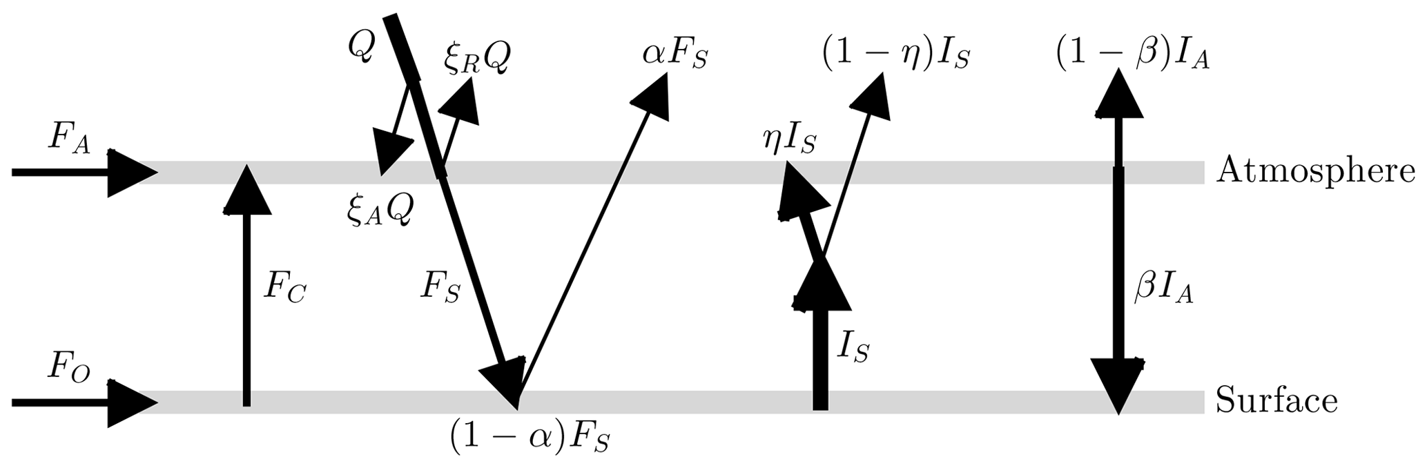
Figure 1 A visualization of the energy balance model (EBM). Here Q is the incident solar radiation. A fraction ξ_A of Q is absorbed by the atmosphere and another fraction ξ_R is reflected by clouds into space. The resulting solar forcing that strikes the surface is $F_{\mathrm{S}}=(\mathrm{1}-{\mathit{\xi }}_{\mathrm{A}}-{\mathit{\xi }}_{\mathrm{R}})Q$. The surface has albedo α, which means that αF_S is reflected back to space and the remaining energy (1−α)F_S is absorbed by the surface. The surface emits longwave radiation of intensity I_S, of which a fraction ηI_S is absorbed by greenhouse gases in the atmosphere and the remainder (1−η)I_S escapes to space. The atmosphere emits longwave radiation I_A, of which a fraction βI_A goes downward to the surface and the remaining fraction (1−β)I_A escapes to space. The three forcing terms (F_A, F_O, F_C) represent atmospheric heat transport, ocean heat transport and vertical conduction/convection heat transport, respectively. Values of these and other parameters are given in Table 1.

Table 1 Summary of variables and parameters used in the EBM. The values of the physical constants (ξ_a, ξ_R, k_C, k_W, G_C, G_W1, G_W2) are as determined in Kypke (2019) and Dortmans et al. (2019).

The EBM of this paper has been kept as simple as possible, while incorporating the nonlinear physical processes that are essential to our exploration of bifurcation behaviour. In that sense, it follows in the tradition of simple energy balance models of Budyko (1968), Sellers (1969), North et al. (1981), and others. However, this EBM is but the first step in the authors' study of a hierarchy of nonlinear models of increasing complexity. That hierarchy is outlined in the concluding Sect. 4.

2 An energy balance model for climate change

The EBM is a simple two-layer model, with layers corresponding to the surface and atmosphere, respectively; see Fig. 1, which is based on Payne et al. (2015), Trenberth et al. (2009), and Wild et al. (2013). The symbols in Fig. 1 are defined in the caption of Fig. 1 and in Table 1. In the EBM of Fig. 1, the surface receives shortwave radiant energy $F_{\mathrm{S}}=(\mathrm{1}-{\mathit{\xi }}_{\mathrm{A}}-{\mathit{\xi }}_{\mathrm{R}})Q$ from the sun, where Q is the incident solar radiation and ξ_A and ξ_R are the fractions of Q absorbed by the atmosphere and reflected back to space by clouds, respectively. The values of ξ_A and ξ_R are obtained from Trenberth et al. (2009) and Wild et al. (2013) (see the appendix and Table 1). At the surface, a fraction αF_S is reflected back to space, where α is the surface albedo, and the remainder, (1−α)F_S, is absorbed by the surface. The surface re-emits longwave radiant energy of intensity $I_{\mathrm{S}}=\mathit{\sigma }{T}_{\mathrm{S}}^{\mathrm{4}}$ (Stefan–Boltzmann law) upward into the atmosphere. The atmosphere contains greenhouse gases that absorb a fraction η of the radiant energy I_S from the surface, and the remainder, (1−η)I_S, escapes to space. The atmosphere re-emits radiant energy of total intensity I_A. Of this radiation I_A, a fraction βI_A is directed downward to the surface, and the remaining fraction (1−β)I_A goes upward and escapes to space. Balancing the energy flows represented in Fig. 1 leads directly to the following dynamical system:

$$\begin{array}{ll}{\displaystyle }{c}_{\mathrm{S}}{\displaystyle \frac{\mathrm{d}{T}_{\mathrm{S}}}{\mathrm{d}t}}=& {\displaystyle }(\mathrm{1}-\mathit{\alpha })(\mathrm{1}-{\mathit{\xi }}_{\mathrm{A}}-{\mathit{\xi }}_{\mathrm{R}})Q+F_O+\mathit{\beta }{I}_{\mathrm{A}}\\ \text{(1)}& {\displaystyle }& {\displaystyle }-\mathit{\sigma }{T}_{\mathrm{S}}^{\mathrm{4}}-F_{\mathrm{C}},\text{(2)}& {\displaystyle }{c}_{\mathrm{A}}{\displaystyle \frac{\mathrm{d}{I}_{\mathrm{A}}}{\mathrm{d}t}}=& {\displaystyle }{F}_{\mathrm{A}}+\mathit{\eta }\mathit{\sigma }{T}_{\mathrm{S}}^{\mathrm{4}}-I_{\mathrm{A}}+F_{\mathrm{C}}+{\mathit{\xi }}_{\mathrm{A}}Q,\end{array}$$

where Eq. (1) represents surface energy balance and Eq. (2) represents atmosphere energy balance. Here c_S and c_A are specific heat rate constants derived in Kypke (2019) and Kypke and Langford (2020) and listed in Table 1. There are three heat transport terms: F_A is atmospheric heat transport, F_O is ocean heat transport (both horizontally), and F_C is conductive/convective heat transport, vertically from the surface to the atmosphere.

In Eqs. (1) and (2) there is an asymmetry, in that temperature T_S is used to represent the state of the surface in Eq. (1), but radiant energy intensity I_A is used instead of temperature to represent the state of the atmosphere in Eq. (2). Note that either temperature variables or energy intensity variables could have been used in either equation if we assume the Stefan–Boltzmann law ($I_{\mathrm{S}}=\mathit{\sigma }{T}_{\mathrm{S}}^{\mathrm{4}}$ and $I_{\mathrm{A}}=\mathit{ϵ}\mathit{\sigma }{T}_{\mathrm{A}}^{\mathrm{4}}$, where ϵ=0.9 is the emissivity of dry air). The use of T_S as state variable in surface Eq. (1) is the obvious choice, since the surface temperature is the most important variable in the EBM. However, the choice of I_A instead of T_A in Eq. (2) is less obvious. The atmosphere has thickness. In the actual atmosphere, temperature decreases with height above the surface at a rate called the lapse rate. Therefore, there is not just one value of temperature T_A for the atmosphere. However, we can define a single value of radiant energy intensity I_A, corresponding to the total energy emitted vertically by the slab of atmosphere, and use this instead of temperature in the energy balance Eq. (2). A second reason for the use of I_A instead of T_A in Eq. (2) is that this facilitates the use of the ICAO Standard Atmosphere lapse rate, as explained in the paragraph following Eqs. (4) and (5) below, and that allows for a more realistic representation of the greenhouse gas behaviour of water vapour.

The first step of the analysis of system Eqs. (1) and (2) is a rescaling of temperature T (in kelvin) to a new nondimensional temperature τ with τ=1 corresponding to the freezing temperature of water (T_R=273.15 K). Then all variables and parameters in the system can be made nondimensional by the scalings

$$\begin{array}{ll}{\displaystyle }{\mathit{\tau }}_{\mathrm{A}}& {\displaystyle }={\displaystyle \frac{T_{\mathrm{A}}}{T_{\mathrm{R}}}},{\mathit{\tau }}_{\mathrm{S}}={\displaystyle \frac{T_{\mathrm{S}}}{T_{\mathrm{R}}}},q={\displaystyle \frac{Q}{\mathit{\sigma }{T}_{\mathrm{R}}^{\mathrm{4}}}},f_{\mathrm{O}}={\displaystyle \frac{F_{\mathrm{O}}}{\mathit{\sigma }{T}_{\mathrm{R}}^{\mathrm{4}}}},\\ \text{(3)}& {\displaystyle }{f}_{\mathrm{A}}& {\displaystyle }={\displaystyle \frac{F_{\mathrm{A}}}{\mathit{\sigma }{T}_{\mathrm{R}}^{\mathrm{4}}}},f_{\mathrm{C}}={\displaystyle \frac{F_{\mathrm{C}}}{\mathit{\sigma }{T}_{\mathrm{R}}^{\mathrm{4}}}},i_{\mathrm{A}}={\displaystyle \frac{I_{\mathrm{A}}}{\mathit{\sigma }{T}_{\mathrm{R}}^{\mathrm{4}}}},\mathit{\omega }={\displaystyle \frac{\mathrm{\Omega }}{T_{\mathrm{R}}}},{\displaystyle }s& {\displaystyle }={\displaystyle \frac{\mathit{\sigma }{T}_{\mathrm{R}}^{\mathrm{3}}}{C_{\mathrm{S}}}}\cdot t,\mathit{\chi }={\displaystyle \frac{C_{\mathrm{S}}}{C_{\mathrm{A}}\mathit{\sigma }{T}_{\mathrm{R}}^{\mathrm{3}}}}=\mathrm{54.26},\end{array}$$

where s is dimensionless time and χ is the dimensionless heat rate constant. The surface and atmosphere energy balance Eqs. (1) and (2) in nondimensional variables are then

$$\begin{array}{ll}{\displaystyle \frac{\mathrm{d}{\mathit{\tau }}_{\mathrm{S}}}{\mathrm{d}s}}=& {\displaystyle }(\mathrm{1}-\mathit{\alpha }({\mathit{\tau }}_{\mathrm{S}}\left)\right)(\mathrm{1}-{\mathit{\xi }}_{\mathrm{A}}-{\mathit{\xi }}_{\mathrm{R}})q\\ \text{(4)}& {\displaystyle }& {\displaystyle }+f_O+\mathit{\beta }{i}_{\mathrm{A}}-{\mathit{\tau }}_{\mathrm{S}}^{\mathrm{4}}-f_{\mathrm{C}},\text{(5)}& {\displaystyle \frac{\mathrm{1}}{\mathit{\chi }}}{\displaystyle \frac{\mathrm{d}{i}_{\mathrm{A}}}{\mathrm{d}s}}=& {\displaystyle }{f}_{\mathrm{A}}+\mathit{\eta }({\mathit{\tau }}_{\mathrm{S}};\mathit{\mu },\mathit{\delta }){\mathit{\tau }}_{\mathrm{S}}^{\mathrm{4}}-i_{\mathrm{A}}+f_{\mathrm{C}}+{\mathit{\xi }}_{\mathrm{A}}q.\end{array}$$

In Fig. 1, the atmosphere is shown to be a uniform slab, even though the actual atmosphere is not a uniform slab. The essential nonlinear processes in the atmosphere, which the model must capture, are the heating effects of the greenhouse gases CO₂ and H₂O. According to the Beer–Lambert law, the absorptivity of these gases is determined by their optical depths. Therefore, in the model we substitute for optical depth in the slab, the values of optical depth that these gases would have in the ICAO Standard Atmosphere (ICAO, 1993), which is a good approximation to the actual atmosphere. In the ICAO model, the rate of change of temperature with altitude is assumed to be a negative constant −Γ, called the ICAO lapse rate; see Table 1. The concentration of CO₂ is independent of temperature, but the concentration of H₂O decreases with altitude as the temperature decreases, according to the Clausius–Clapeyron relation (Pierrehumbert, 2010). Then the optical depth of H₂O is obtained by integration of the Clausius–Clapeyron relation from the surface to the tropopause, resulting in Eq. (6). In this way, the simple slab model has greenhouse effects close to those of these two gases in the actual atmosphere, where the temperature is not constant but decreases with altitude. This use of the ICAO lapse rate differentiates the present EBM from all previous EBMs in the literature. The calculation gives the absorptivity η due to greenhouse gases, in the atmosphere Eqs. (2) or (5), as

$$\begin{array}{ll}{\displaystyle }\mathit{\eta }({\mathit{\tau }}_{\mathrm{S}};\mathit{\mu },\mathit{\delta })=& {\displaystyle }\mathrm{1}-\exp [-\mathit{\mu }{G}_{\mathrm{C}}-\mathit{\delta }{G}_{\text{W2}}\cdot \\ \text{(6)}& {\displaystyle }& {\displaystyle }\underset{{\mathit{\tau }}_{\mathrm{S}}-\mathit{\gamma }Z}{\overset{{\mathit{\tau }}_s}{\int }}{\displaystyle \frac{\mathrm{1}}{\mathit{\tau }}}\exp \left(G_{\text{W1}}\right[{\displaystyle \frac{\mathit{\tau }-\mathrm{1}}{\mathit{\tau }}}\left]\right)d\mathit{\tau }],\end{array}$$

where μ is the concentration of CO₂ in the atmosphere, measured in molar parts per million; δ is the relative humidity of water vapour $(\mathrm{0}\le \mathit{\delta }\le \mathrm{1})$; $\mathit{\gamma }=\mathrm{\Gamma }/T_{\mathrm{R}}$ is the nondimensionalized lapse rate (ICAO, 1993); and Z is the tropopause height. (Since methane acts similarly to carbon dioxide as a greenhouse gas, it may be assumed that μ includes also the effects of methane.) Equation (6) is derived using fundamental laws of atmospheric physics: the Beer–Lambert law, the ideal gas law and the Clausius–Clapeyron equation; see Dortmans et al. (2019) for more details. In Eq. (6),

$$\begin{array}{ll}{\displaystyle }{G}_{\mathrm{C}}& {\displaystyle }={\displaystyle \frac{\mathrm{1.52}{k}_{\mathrm{c}}{P}_{\mathrm{A}}}{{\mathrm{10}}^{\mathrm{6}}g}},G_{\text{W1}}={\displaystyle \frac{L_{\mathrm{v}}}{R_{\mathrm{W}}{T}_{\mathrm{R}}}},\\ \text{(7)}& {\displaystyle }& {\displaystyle }\text{and}{G}_{\text{W2}}={\displaystyle \frac{k_{\mathrm{W}}\cdot T_{\mathrm{R}}\cdot {\mathit{\rho }}^{\text{sat}}\left(T_{\mathrm{R}}\right)}{\mathrm{\Gamma }}}\end{array}$$

are dimensionless physical constants determined in Dortmans et al. (2019), and k_C and k_W are absorption coefficients for CO₂ and H₂O, respectively; see Table 1.

In the surface Eqs. (1) or (4), α is the albedo of the surface $(\mathrm{0}\le \mathit{\alpha }\le \mathrm{1})$ and α depends strongly on temperature τ_S near the freezing point (τ_S=1). Typical values of surface albedo are 0.6–0.9 for snow, 0.4–0.7 for ice, 0.2 for crop land, and 0.1 or less for open ocean. Therefore, in the high Arctic, as the ice-cover melts, the albedo will transition from a high value such as α_c=0.7 for snow/ice to a low value such as α_w=0.08 for open ocean. Some authors have assumed this change in albedo to be a discontinuous step function (Dortmans et al., 2018). However, all variables in this EBM have annually averaged values. As the Arctic thaws, the annual average albedo will transition gradually, over a number of years, from its high value for year-round ice-covered surface to its low value for year-round open ocean. Therefore, in this paper we use a smoothly varying albedo function, which better models this gradual transition from high to low albedo, as the mean temperature rises through the freezing point (τ_S=1). It is modelled by the hyperbolic tangent function:

$$\begin{array}{}\text{(8)}& \mathit{\alpha }({\mathit{\tau }}_{\mathrm{S}},\mathit{\omega })={\displaystyle \frac{\mathrm{1}}{\mathrm{2}}}\left(\right[{\mathit{\alpha }}_{\mathrm{w}}+{\mathit{\alpha }}_{\mathrm{c}}]+[{\mathit{\alpha }}_{\mathrm{w}}-{\mathit{\alpha }}_{\mathrm{c}}\left]\tanh \right({\displaystyle \frac{{\mathit{\tau }}_{\mathrm{S}}-\mathrm{1}}{\mathit{\omega }}}\left)\right).\end{array}$$

Here the parameter ω controls the steepness of this switch function. Analysis of polar ice data in recent years confirms that this function gives a good fit to the decline of ice cover and albedo in the Arctic with $\mathit{\omega }=\mathrm{\Omega }/T_{\mathrm{R}}=\mathrm{0.01}$ (Pistone et al., 2014; Dortmans et al., 2019). The dependence of Arctic Ocean sea-ice thickness on surface albedo parametrization in models has been investigated in Björk et al. (2013), where alternative albedo schemes are compared. The nonlinear dependence of albedo on temperature, as in Eq. (8), has been shown to lead to hysteresis behaviour (Stranne et al., 2014; Dortmans et al., 2019).

2.1 Refinement of the paleoclimate EBM to an Anthropocene EBM

Paleoclimate data are difficult to obtain and in general can only be inferred from proxy data. The situation is different for the Anthropocene. There is now an abundance of land-based and satellite climate data. Therefore, the EBM in this paper can be refined to take advantage of the additional data. The appendix details the changes made in this EBM from that which was presented in Dortmans et al. (2019) and Kypke and Langford (2020), to improve its accuracy for the Anthropocene. These changes do not change the fundamental behaviour of the EBM, including the existence of bifurcations, but they do make the numerical predictions more reliable. Table 1 of this paper may be compared with the corresponding Table 1 of Kypke and Langford (2020) to see how parameter values have been updated.

The total absorptivity η, given in Eq. (6) for paleoclimates, is now modified to reflect the fact that clouds absorb a fraction η_Cl of the outgoing longwave radiation. In this paper

$$\begin{array}{ll}{\displaystyle }\mathit{\eta }({\mathit{\tau }}_{\mathrm{S}},\mathit{\mu },\mathit{\delta })=& {\displaystyle }\mathrm{1}-(\mathrm{1}-{\mathit{\eta }}_{\text{Cl}})\cdot \exp [-\mathit{\mu }{G}_{\mathrm{C}}-\mathit{\delta }{G}_{\text{W2}}\cdot \\ \text{(9)}& {\displaystyle }& {\displaystyle }\underset{{\mathit{\tau }}_{\mathrm{S}}-\mathit{\gamma }Z}{\overset{{\mathit{\tau }}_s}{\int }}{\displaystyle \frac{\mathrm{1}}{\mathit{\tau }}}\exp \left(G_{\text{W1}}\right[{\displaystyle \frac{\mathit{\tau }-\mathrm{1}}{\mathit{\tau }}}\left]\right)\mathrm{d}\mathit{\tau }];\end{array}$$

see the appendix.

The vertical heat transport term F_C has been modified to take into account both sensible and latent heat transport (Kypke, 2019). See the appendix, where the following formula is obtained (here in nondimensional form).

$$\begin{array}{ll}{\displaystyle }{f}_{\mathrm{C}}\left({\mathit{\tau }}_{\mathrm{S}}\right)=& {\displaystyle \frac{H_{\mathrm{1}}\mathit{\gamma }Z}{({\mathit{\tau }}_{\mathrm{S}}-\mathit{\gamma }Z)}}+{\displaystyle \frac{H_{\mathrm{2}}}{({\mathit{\tau }}_{\mathrm{S}}-\mathit{\gamma }Z)}}\cdot \\ \text{(10)}& {\displaystyle }& {\displaystyle }(e^{\left[G_{\text{W1}}\frac{{\mathit{\tau }}_{\mathrm{S}}-\mathrm{1}}{{\mathit{\tau }}_{\mathrm{S}}}\right]}-\mathit{\delta }{e}^{\left[G_{\text{W1}}\frac{{\mathit{\tau }}_{\mathrm{S}}-\mathit{\gamma }Z-\mathrm{1}}{{\mathit{\tau }}_{\mathrm{S}}-\mathit{\gamma }Z}\right]}),\end{array}$$

where H₁ and H₂ are nondimensional constants:

$${\displaystyle }{\displaystyle }{H}_{\mathrm{1}}={\displaystyle \frac{C_{\mathrm{D}}U{c}_{\mathrm{P}}{P}_{\mathrm{0}}}{\mathit{\sigma }{T}_{\mathrm{R}}^{\mathrm{4}}{R}_{\mathrm{A}}}}\text{and}{H}_{\mathrm{2}}={\displaystyle \frac{C_{\mathrm{D}}U{L}_{\mathrm{v}}{P}^{\text{sat}}\left(T_{\mathrm{R}}\right)}{\mathit{\sigma }{T}_{\mathrm{R}}^{\mathrm{5}}{R}_{\mathrm{W}}}}.$$

In Eqs. (4) and (5), at equilibrium (i.e. $\frac{\mathrm{d}\cdot }{\mathrm{d}\widehat{s}}=\mathrm{0}$), the state variable i_A is easily eliminated, leaving a single equation with a single state variable τ_S,

$$\begin{array}{ll}{\displaystyle }\mathrm{0}=& {\displaystyle }(\mathrm{1}-\mathit{\alpha }({\mathit{\tau }}_{\mathrm{S}}\left)\right)(\mathrm{1}-{\mathit{\xi }}_{\mathrm{A}}-{\mathit{\xi }}_{\text{Cl}})q+f_{\mathrm{O}}+\mathit{\beta }{f}_{\mathrm{A}}\\ \text{(11)}& {\displaystyle }& {\displaystyle }-f_{\mathrm{C}}(\mathrm{1}-\mathit{\beta })+\mathit{\beta }q{\mathit{\xi }}_{\mathrm{A}}-{\mathit{\tau }}_{\mathrm{S}}^{\mathrm{4}}(\mathrm{1}-\mathit{\beta }\mathit{\eta }({\mathit{\tau }}_{\mathrm{S}}\left)\right).\end{array}$$

2.2 Cusp bifurcation in the EBM

In this subsection, we outline the proof that the cusp bifurcation, which was proven to exist in the Paleoclimate EBM (Kypke and Langford, 2020), in fact persists in this Anthropocene EBM Eqs. (4) and (5). Therefore, the conclusions of that paper carry over to this paper. Readers not interested in these mathematical details may skip this subsection.

The right-hand sides of Eqs. (4) and (5) can be represented by a single vector function $F:{\mathbb{R}}^{\mathrm{2}}\times {\mathbb{R}}^{\mathrm{4}}\to {\mathbb{R}}^{\mathrm{2}}$. Then an equilibrium point $({\overline{\mathit{\tau }}}_{\mathrm{S}},{\overline{i}}_{\mathrm{A}})$ of Eqs. (4) and (5), at which $\frac{\mathrm{d}{\mathit{\tau }}_{\mathrm{S}}}{\mathrm{d}t}=\frac{\mathrm{d}{i}_{\mathrm{A}}}{\mathrm{d}t}=\mathrm{0}$, is a solution of

$$\begin{array}{}\text{(12)}& F({\overline{\mathit{\tau }}}_{\mathrm{S}},{\overline{i}}_{\mathrm{A}};\mathit{\rho })=\mathrm{0},\end{array}$$

where ρ represents four physical parameters that may be varied in the model,

$$\begin{array}{}\text{(13)}& \mathit{\rho }\equiv \mathit{\{}\mathit{\mu },\mathit{\delta },F_{\mathrm{O}},\mathit{\omega }\mathit{\}}.\end{array}$$

See Table 1 for definitions of these parameters. Since the codimension of the cusp bifurcation is only two, there is some redundancy in the choice of these four parameters. For application to future climates, the parameter pair (F_O,μ) is of primary interest. Equilibrium points $({\overline{\mathit{\tau }}}_{\mathrm{S}},{\overline{i}}_{\mathrm{A}})$ satisfying Eq. (12) have been computed in Kypke (2019). Having computed the equilibrium point $({\overline{\mathit{\tau }}}_{\mathrm{S}},{\overline{i}}_{\mathrm{A}})$ satisfying Eq. (12), the system may be translated to the origin $(x,y)=(\mathrm{0},\mathrm{0})$, in new state variables defined by

$${\displaystyle }{\displaystyle }(x,y)\equiv ({\mathit{\tau }}_{\mathrm{S}}-{\overline{\mathit{\tau }}}_{\mathrm{S}},i_{\mathrm{A}}-{\overline{i}}_{\mathrm{A}}),$$

and Eqs. (4) and (5) become

$$\begin{array}{ll}{\displaystyle \frac{\mathrm{d}x}{\mathrm{d}s}}=& {\displaystyle }(\mathrm{1}-\mathit{\alpha })(\mathrm{1}-{\mathit{\xi }}_{\mathrm{A}}-{\mathit{\xi }}_{\text{Cl}})q+f_{\mathrm{O}}-f_{\mathrm{C}}\\ {\displaystyle }& {\displaystyle }+\mathit{\beta }(y+{\overline{i}}_{\mathrm{A}})-(x+{\overline{\mathit{\tau }}}_{\mathrm{S}}{)}^{\mathrm{4}},\\ \text{(14)}& {\displaystyle \frac{\mathrm{d}y}{\mathrm{d}s}}=& {\displaystyle }\mathit{\chi }\left[f_{\mathrm{A}}+f_{\mathrm{C}}+q{\mathit{\xi }}_{\mathrm{A}}+\mathit{\eta }(x+{\overline{\mathit{\tau }}}_{\mathrm{S}}{)}^{\mathrm{4}}-(y+{\overline{i}}_{\mathrm{A}})\right].\end{array}$$

For Eq. (14) to have a steady-state bifurcation at the equilibrium point (0,0), the Jacobian J of F in Eq. (12) must have a zero eigenvalue, λ₁=0, at that point. (A Hopf bifurcation is not possible in this system.) For stability, the second eigenvalue satisfies λ₂<0. The corresponding eigenvectors, e₁,e₂, form an eigenbasis. A linear transformation takes (x,y) coordinates to eigenbasis coordinates (u,v), where $(x,y)=\mathbf{T}(u,v)$, and the columns of T are the normalized eigenvectors e₁,e₂ in Eq. (17), below. Then in (u,v) coordinates, the 2-D system Eq. (14) becomes

$$\begin{array}{ll}{\displaystyle \frac{\mathrm{d}u}{\mathrm{d}s}}=& {\displaystyle }{\displaystyle \frac{\mathrm{1}}{\mathit{\varphi }}}\left[\right(\mathrm{1}-\mathit{\alpha }\left)\right(\mathrm{1}-{\mathit{\xi }}_{\mathrm{A}}-{\mathit{\xi }}_{\text{Cl}})q+f_{\mathrm{O}}+\mathit{\beta }{f}_{\mathrm{A}}\\ \text{(15)}& {\displaystyle }& {\displaystyle }-(\mathrm{1}-\mathit{\beta })f_{\mathrm{C}}+\mathit{\beta }{\mathit{\xi }}_{\mathrm{A}}q+(\mathrm{1}-\mathit{\beta }\mathit{\eta })(u-kv+{\overline{\mathit{\tau }}}_{\mathrm{S}}{)}^{\mathrm{4}}]{\displaystyle \frac{\mathrm{d}v}{\mathrm{d}s}}=& {\displaystyle \frac{\mathrm{1}}{\mathit{\varphi }}}[-\mathrm{\ell }[(\mathrm{1}-\mathit{\alpha })(\mathrm{1}-{\mathit{\xi }}_{\mathrm{A}}-{\mathit{\xi }}_{\text{Cl}})q+f_{\mathrm{O}}]\\ {\displaystyle }& {\displaystyle }+(\mathrm{\ell }+\mathit{\chi })f_{\mathrm{C}}+\mathit{\chi }{f}_{\mathrm{A}}-(\mathrm{\ell }\mathit{\beta }+\mathit{\chi })[\mathrm{\ell }u+v+{\overline{i}}_{\mathrm{A}}]\\ {\displaystyle }& {\displaystyle }+(\mathrm{\ell }+\mathit{\chi }\mathit{\eta })(u-kv+{\overline{\mathit{\tau }}}_{\mathrm{S}}{)}^{\mathrm{4}}],\end{array}$$

where

$$\begin{array}{}\text{(16)}& \mathrm{\ell }=f_{C\mathrm{0}}^{\prime }+\mathrm{4}{\mathit{\eta }}_{\mathrm{0}}{\overline{\mathit{\tau }}}_{\mathrm{S}}^{\mathrm{3}}+{\mathit{\eta }}_{\mathrm{0}}^{\prime }{\overline{\mathit{\tau }}}_{\mathrm{S}}^{\mathrm{4}},k={\displaystyle \frac{\mathit{\beta }}{\mathit{\chi }}},\mathit{\varphi }=\mathrm{1}+k\mathrm{\ell }\end{array}$$

and

$$\begin{array}{}\text{(17)}& {\mathit{e}}_{\mathrm{1}}=\left(\begin{array}{c}\mathrm{1}\\ \mathrm{\ell }\end{array}\right),{\mathit{e}}_{\mathrm{2}}=\left(\begin{array}{c}-k\\ \mathrm{1}\end{array}\right).\end{array}$$

Recall that the parameters μ and δ, representing CO₂ concentration and water vapour relative humidity, respectively, enter into Eq. (15) through the function η defined in Eq. (9). For more details, see Kypke (2019), Kypke and Langford (2020), and Kuznetsov (2004).

If the Centre Manifold Theorem applies to Eq. (15), then there exists a flow-invariant centre manifold, which is tangent to the u axis. The applicability of this theorem has been verified, and the centre manifold has been computed for the present Anthropocene EBM as was done for the paleoclimate EBM in Kypke (2019) and Kypke and Langford (2020). Details are omitted here. A phase portrait for Eq. (15) in a neighbourhood of the cusp equilibrium point, together with a portion of this centre manifold (in red), is shown in Fig. 2 in (u,v) coordinates. In this figure, trajectories quickly collapse to the centre manifold around the equilibrium point (0,0), as predicted by the Centre Manifold Theorem. The cusp equilibrium manifold for Eq. (15) in normal form is shown in Fig. 3. Here ζ₁ and ζ₂ are the normal form unfolding parameters for the cusp bifurcation. Note the coexistence of three equilibrium points with different values of u (two stable and the middle one unstable) inside the cusp-shaped region, but only one equilibrium point (stable) outside of that region.

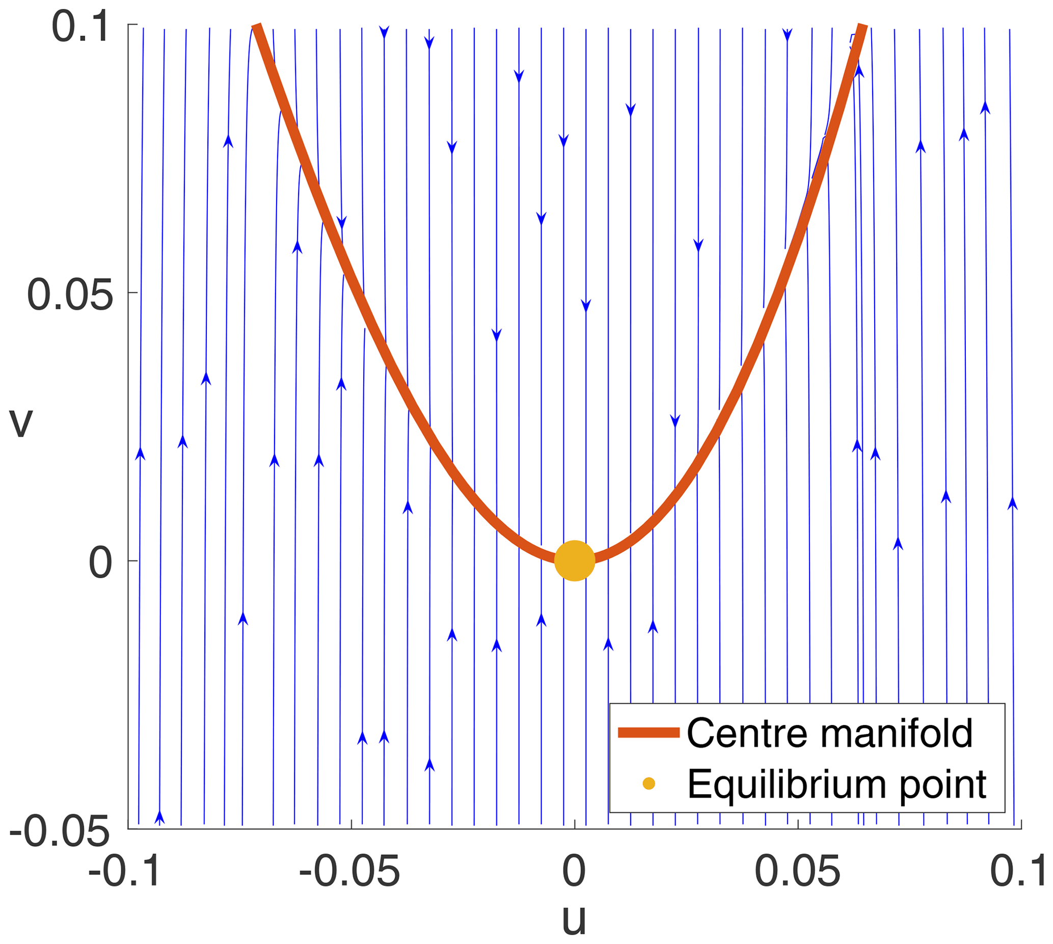
Figure 2 Phase portrait of system Eq. (15), together with a portion of the centre manifold (in red), in the (u,v) eigenbasis coordinates. Parameter values are those at the computed cusp point. The yellow dot marks the cusp equilibrium point. Note the rapid approach to the centre manifold from initial points not on the centre manifold in contrast to the slow evolution along the centre manifold.

Figure 3 Cusp bifurcation diagram for the EBM in normal form coordinates. (a) Graph of the equilibrium surface with normal form unfolding parameters (ζ₁,ζ₂). (b) Projection of this surface in 3-D onto the (ζ₁,ζ₂) plane. The blue semi-cubic parabola represents fold bifurcations, and it separates the (ζ₁,ζ₂) plane into two open 2-D regions. Inside the cusp region, that is between the two branches of the semi-cubic parabola, there exist three equilibrium solutions u: two stable and the middle one unstable. Outside of the semi-cubic parabola there exists only one unique equilibrium solution u and it is stable.

3 Anthropocene climate forecasts

In this section, the EBM of Sect. 2 is applied to the present and future climates of the Earth to investigate the possibility of climate bifurcations (or tipping points) in the Anthropocene. The principal parameters chosen to be explored are carbon dioxide concentration μ, ocean heat transport F_O, and relative humidity δ. The EBM is adapted locally to three separate regions, namely the Arctic, Antarctic, and the tropics, in Sect. 3.2, 3.3, and 3.4, respectively.

Carbon dioxide production due to human activities has been well documented as a driver of climate change in the Anthropocene. Projections of future atmospheric CO₂ levels are available under various future scenarios; we follow the Representative Concentration Pathways of IPCC (2013), which is described in Sect. 3.1. Ocean heat transport is a difficult quantity to predict, as many different factors influence the transport of heat to various regions of the world via the oceans. Changes in temperature can change ocean heat transport which in turn affects local temperatures. This is ocean heat transport feedback, which is explored in Sect. 3.2.2. Similarly, the role of atmospheric heat transport feedback is investigated briefly in Sect. 3.2.2. In addition, water vapour is a powerful greenhouse gas, with a positive feedback effect that is investigated in Sect. 3.2.3.

In Sect. 3.5, a globally averaged model is considered, mainly for the purpose of determining the global equilibrium climate sensitivity (ECS) of this EBM, for comparison with the ECS of other models as reported in IPCC (2013) and Priostosescu and Huybers (2017); see Sect. 3.6.

3.1 Representative Concentration Pathways (RCPs)

The IPCC has standardized four Representative Concentration Pathways (RCPs), which are used for projections of future carbon dioxide concentrations; see van Vuuren et al. (2011) and Box TS.6 in IPCC (2013). These RCPs are scenarios for differing levels of anthropogenic forcings on the climate of the Earth and represent differing global societal and political “storylines”. The scenarios are named RCP 8.5, RCP 6.0, RCP 4.5, and RCP 2.6, after their respective peak radiative forcing increases in the 21st century. That is, in the year 2100, RCP 8.5 will reach its maximum radiative forcing due to anthropogenic emissions of +8.5 W m⁻² relative to the year 1750. This scenario is understood as one where emissions continue to rise and are not mitigated in any way. RCP 6.0 corresponds to +6.0 W m⁻² and RCP 4.5 corresponds to +4.5 W m⁻² relative to 1750. These are stabilization scenarios, where greenhouse gas emissions level off to a target amount by the end of the century. Finally, RCP 2.6 corresponds to +2.6 W m⁻² in 2100, relative to 1750. This is a mitigation scenario, where strong steps are taken to eliminate the increase and eventually reduce anthropogenic greenhouse gas emissions. Figure 4 shows the carbon dioxide concentrations projected to the year 2500 in the IPCC scenarios for the four RCPs. The carbon dioxide increase is relatively moderate for RCPs 2.6 and 4.5 and even decreasing eventually for RCP 2.6. The increase for RCP 6.0 is larger, and it is drastic for RCP 8.5.

Figure 4 Carbon dioxide concentration μ, as projected by the IPCC for each of the four RCP hypothetical scenarios. This figure is generated from data at IIASA (2019).

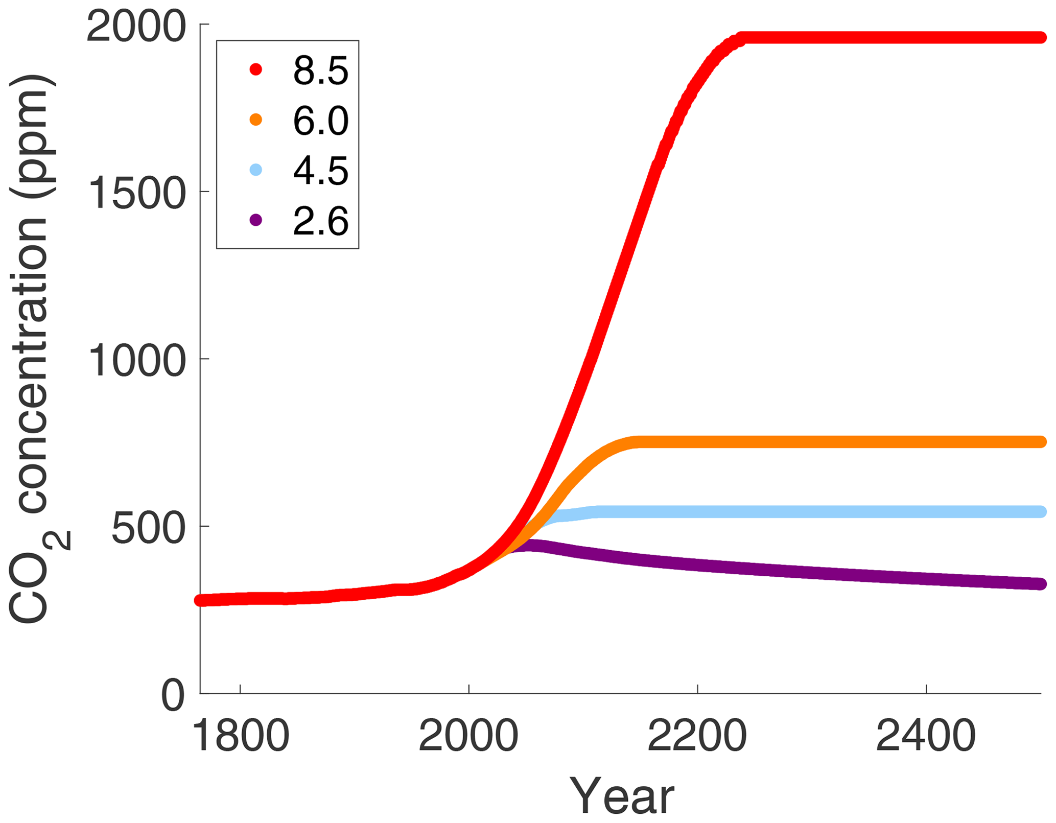
These RCPs represent hypothetical forcings due to human activity up to the year 2100. Beyond 2100, they assume a “constant composition commitment”, where emissions are kept constant, which serves to stabilize the scenarios beyond 2100 (IPCC, 2013). Of course, emissions could continue to increase or be greatly reduced (“zero emissions commitment”) at some point in the future. However, the constant emission commitment dataset provided in IPCC (2013), and shown in Fig. 4, is what is utilized in this work. In the following sections we enter the CO₂ concentrations μ shown in Fig. 4, one at a time along each of the four IPCC RCPs, into the versions of our EBM for the Arctic. Antarctic, etc., and we then let the EBM climate evolve quasi-statically along each CO₂ pathway.

3.2 EBM for the Anthropocene Arctic

Figure 5a is the manifold of equilibrium states for the EBM parameterized by (F_O,μ) for the case of an Arctic climate under Anthropocene conditions. Figure 5b is the projection of this manifold onto the parameter plane, showing the fold bifurcation lines as boundaries between coloured regions. Parameter values are as in Table 1, with F_A=104 W m⁻² and δ=0.6 taken as the nominal values for the modern Arctic throughout this section, except in Fig. 8. These figures were computed as in Kypke and Langford (2020). The cusp point, seen in Fig. 3, still exists but is not visible in Fig. 5, because it is outside of the range of parameters included in the figure.

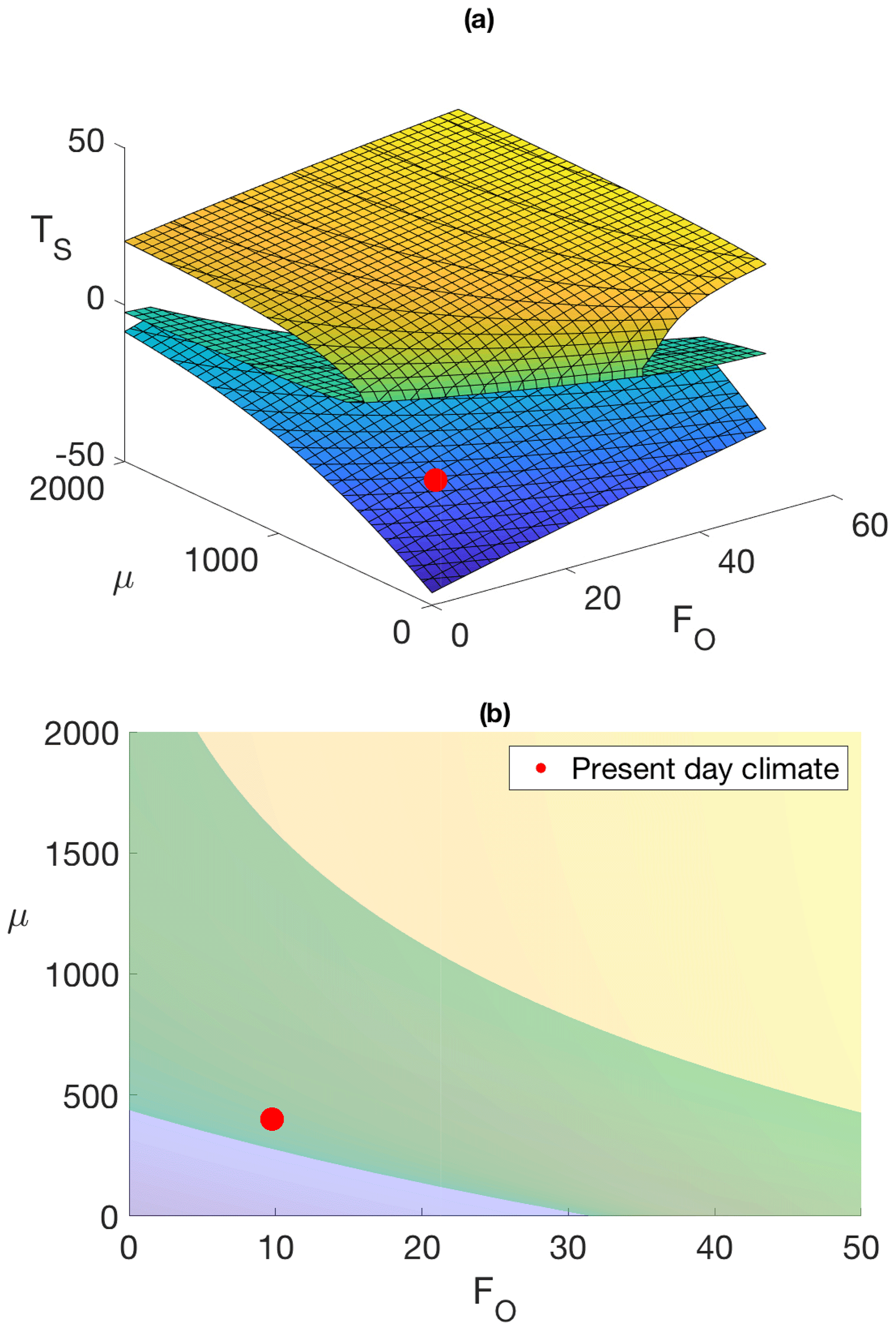
Figure 5 Energy balance model of the modern Arctic. Parameter values are as in Table 1. The red dots locate today's Arctic climate conditions. Ocean heat transport F_O increases from 0 to 50 W m⁻² and carbon dioxide concentration μ increases from 0 to 2000 ppm. (a) 3-D plot of equilibrium manifold. (b) Projection on the (F_O,μ) parameter plane.

In Fig. 5a, today's climate state lies on the lower (blue) portion of the equilibrium manifold, as shown by the red dot. The upper (yellow) portion represents a coexisting warm equable climate state, similar to the climate of Earth in the Pliocene and earlier. The intermediate (green) portion represents an unstable (and unobservable) climate state.

Similarly, in Fig. 5b, the blue area represents unique cold stable states, yellow represents unique warm stable states, and the green region is the overlap region between the two fold bifurcations, where both warm and cold states coexist. Hence, on moving in the (F_O,μ) parameter space starting from the blue region, crossing the green region, and into the yellow region, there would be no observable change in climate on crossing from blue to green; however, crossing the boundary from green to yellow would cause a catastrophic jump from cold to warm stable climate states. Alternatively, if the (F_O,μ) parameter values moved from the yellow, through the green, into the blue region in Fig. 5b, there would be no abrupt change in climate state on crossing the yellow–green boundary, but a sudden transition to a cold state would occur at the green–blue boundary. This behaviour is called hysteresis.

3.2.1 Arctic climate for the four RCPs

The paramount question considered in this paper can now be phrased as follows. Can a bifurcation leading to a warmer and more equable climate state be expected in the EBM if it is allowed to evolve along one of the four RCPs in Fig. 4? In Fig. 5b, this bifurcation would correspond to crossing the line of fold bifurcations separating the green and yellow regions on increasing μ and possibly F_O.

Figure 6 shows the increase in surface temperature in the Arctic region, using historical data from the year 1900 to the present, and then the EBM forecasts up to the years 2100 and 2300, holding μ to each of the four RCPs in Fig. 4, and with constants $F_{\mathrm{O}}=\mathrm{10}\mathrm{W}{\mathrm{m}}^{-\mathrm{2}}$, F_A = 104 W m⁻², and δ=0.6. The temperature change shown is relative to the Arctic temperature of the EBM in the year 2000, which was −28.90 ^∘C (τ_S=0.8942).

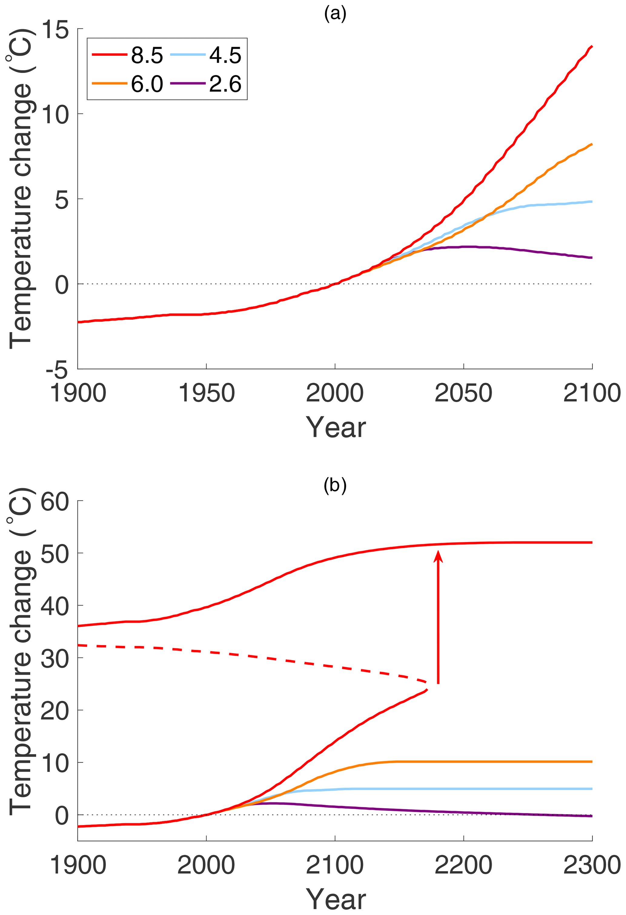
Figure 6 Arctic surface temperature change, relative to the year 2000 average temperature of $-\mathrm{28.90}{}^{\circ }\mathrm{C}$, for each of the four RCPs with constant $F_{\mathrm{O}}=\mathrm{10}\mathrm{W}{\mathrm{m}}^{-\mathrm{2}}$ and with δ=0.6. In (a), the EBM temperature change is projected to year 2100, and in (b) it is projected to year 2300, following the assumptions of the RCP pathways in Fig. 4. Note the dramatic jump in temperature on RCP 8.5, resulting from a saddle-node bifurcation, predicted near the year 2170. The vertical arrow is not an actual trajectory of the dynamical system but rather represents the transition to a new equilibrium state that occurs after the disappearance of the saddle node.

Figure 6a may be compared to the results in Figs. AI.8 and AI.9 in IPCC (2013). Those figures use the RCPs of Fig. 4 and an ensemble of climate models to forecast surface temperature changes for the Arctic up to the year 2100 for land and sea separately. IPCC Fig. AI.8 displays the winter months of December–February and AI.9 is for June–August. Figure 6 of this paper does not distinguish surface covering, so it is given as an annual average value. Figure 6a shows predictions of the EBM to the year 2100, which is the same time frame as for the IPCC GCM projections. Both use the RCP scenarios to determine hypothetical CO₂ concentrations (μ) by year, up to year 2100. Then both use these CO₂ concentrations as input to the respective models (EBM or GCM) to determine predicted climate changes for the same period. They are in good agreement if a weighted average of the sea and land temperature changes are considered and if the winter months are more representative of an annual value for the Arctic climate.

Supported by the agreement until year 2100 between Fig. 6a and the IPCC reported values of temperature change on the RCP paths, the EBM forecast was then extended to the year 2300 (see Fig. 6b), which uses the same parameter values as Fig. 6a. It exhibits a saddle-node bifurcation for RCP 8.5 near the year 2170. Following the disappearance of the cooler equilibrium state in this saddle-node bifurcation, bifurcation theory tells us that there exists a neighbourhood in the state space, where the saddle node once existed, inside of which trajectories move slowly through a so-called “ghost equilibrium” that is a remnant of the saddle node. (The transit time has inverse square-root dependence on the unfolding parameter in that neighbourhood.) Outside of that neighbourhood, trajectories evolve with velocity determined by c_S and c_A in Eqs. (1) and (2) to the upper stable equilibrium point. (The vertical arrow in Fig. 6b represents that transition but is not an actual solution of the dynamical system, and similarly for the vertical arrows in Figs. 7 and 10.) This bifurcation on RCP 8.5 results in a drastic increase in temperature: the mean Arctic temperature jumps by $+\mathrm{26.5}{}^{\circ }\mathrm{C}$ to the new value of $+\mathrm{22.5}{}^{\circ }\mathrm{C}$. This is warmer than the mean annual Arctic temperature in the Pliocene but is consistent with what existed in the Eocene (Willard et al., 2019). Because of simplifications made in this EBM, these numbers should not be taken literally as quantitatively accurate forecasts; however, the qualitative existence of a dramatic increase in temperature due to a bifurcation must be taken seriously. The topological methods employed in this work ensure that bifurcation in this model is a mathematically persistent feature that will be manifest in all “nearby” models; see Kypke and Langford (2020).

The other three RCPs show no such jump in Fig. 6, and indeed all three stay well below freezing. However, it must be borne in mind that the IPCC assumptions (used here) have all four RCPs levelling off to a target value by the end of this century; see Fig. 4. That may be overly optimistic.

3.2.2 Ocean and atmosphere heat transport feedback

In Fig. 6, the only forcing parameter that was changing was the CO₂ concentration (assumed due to anthropogenic forcing). Now we incorporate changes to ocean and atmosphere heat transport, which may amplify the effects of increasing CO₂ alone.

There is evidence that ocean heat transport, F_O, into the Arctic is increasing. For example, Koenigk and Brodeau (2014) project ocean heat transport above 70 ^∘N to increase from 0.15 PW in 1860 to 0.2 and 0.3 PW in 2100, for RCP 2.6 and 8.5, respectively. At the same time, they find in their model that atmospheric heat transport decreases slightly, from 1.65 PW in 1850 to 1.6 PW (1.5 PW) for RCP 2.6 (RCP 8.5). These authors found that, in a stable climate state that ensures global energy conservation, F_O and F_A tend to be out of phase; see, for example, the coupled climate model in Koenigk and Brodeau (2014). However, Yang et al. (2016) show that in a more realistic situation when the climate is perturbed by both heat and freshwater fluxes, the changes in F_O and F_A may be in phase. We assume the latter situation in this paper; see Fig. 7b.

In our model, climate forcings F_O and F_A are expressed as power per unit area (W m⁻²) determined as follows (see Table 2). First, the surface area of the Arctic region is estimated. The Arctic is taken to be the surface of the Earth above the 70th parallel; as such the surface area is

$$\begin{array}{}\text{(18)}& \text{Arctic Surface Area}=\mathrm{2}\mathit{\pi }{R}^{\mathrm{2}}(\mathrm{1}-\cos \mathit{\theta }),\end{array}$$

where R is the radius of the Earth, 6371 km, and θ is 90^∘ minus the latitude. Hence, the surface area of the Earth above 70 ^∘N is approximately 1.538×10¹³ m². This leads to atmospheric and ocean heat fluxes into the Arctic as summarized in Table 2. Because the change in F_A is small relative to the changes in μ and F_O, F_A is kept constant at an intermediate value of 104 W m⁻² in Figs. 5 to 7a.

Table 2 Atmosphere and ocean heat fluxes into the Arctic as simulated in Koenigk and Brodeau (2014), using the global coupled climate model EC-Earth.

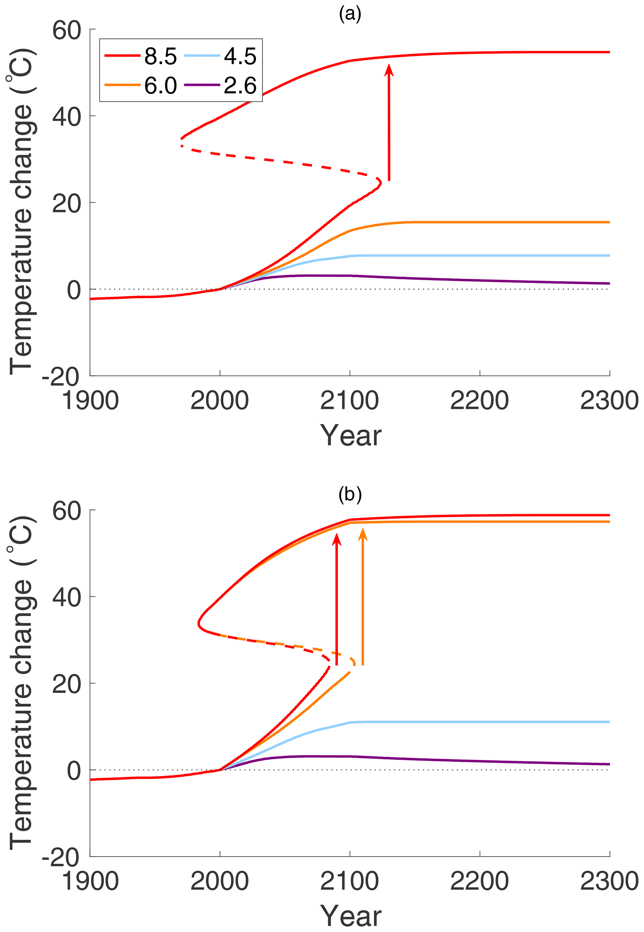
Figure 7 Arctic surface temperature change projected to year 2300 (relative to year 2000 temperature of $-\mathrm{28.90}{}^{\circ }\mathrm{C}$), with linearly increasing ocean heat transport F_O, interpolating the data in Koenigk and Brodeau (2014); see Table 2. (a) With constant F_A=104, the jump in temperature for RCP 8.5 now occurs nearly 40 years earlier than for the case of constant F_O shown in Fig. 6. (b) The same as (a) except that in addition to increasing F_O the atmosphere heat transport F_A also increases, as in Yang et al. (2016), linearly from 104 to 129 W m⁻². Now upward transitions occur on both RCP 8.5 and 6.0, as indicated by the arrows.

Figure 7a shows the change in Arctic surface temperature (relative to the year 2000 temperature of $-\mathrm{28.90}{}^{\circ }\mathrm{C}$) for the four RCPs with the ocean heat flux F_O increasing linearly on each RCP until the year 2100, as projected in Koenigk and Brodeau (2014), using their data for F_O in Table 2 but with constant F_A=104. Beyond the year 2100, until 2300, the ocean heat transport, F_O, , is held constant at its 2100 value. In this scenario, the onset of the jump (via a fold bifurcation) to a warm equable climate is advanced dramatically. The bifurcation for RCP 8.5 occurs in the year 2118, more than 40 years earlier than was the case with a constant F_O in Fig. 6. The temperatures before and after the jump in 2118 between two stable states are −4.6 and +24.7 ^∘C, respectively, which is a sudden increase of 29.3 ^∘C. The other three RCPs remain below the freezing temperature.

Figure 7b shows the same scenario as in 7a, with increasing μ and F_O but with the atmospheric heat transport, F_A, also increasing linearly from 104 W m⁻² in the year 2000 to 129 W m⁻² in 2100, being constant thereafter. In this case, the saddle-node bifurcation occurs even earlier for RCP 8.5, and a new bifurcation appears for RCP 6.0. Both of these changes make mitigation more challenging.

3.2.3 Water vapour feedback

Overall, water vapour is known to be the most powerful greenhouse gas in the atmosphere (Dai, 2006; Pierrehumbert, 2010; IPCC, 2013). Warming of the surface causes evaporation of more water vapour, which causes further greenhouse warming and a further rise in surface temperature. Thus, water vapour amplifies the warming due to other causes. This is called water vapour feedback. Empirical studies such as Dai (2006) show that the increase in surface specific humidity H with surface temperature T is close to that predicted by the Clausius–Clapeyron equation as in Eq. (6) (outside of desert regions). The relative humidity, RH or δ, changes little with surface temperature, even as the specific humidity H increases (Serreze et al., 2012). For paleoclimates, Jahren and Sternberg (2003) have described an Eocene Arctic rain forest with RH estimated to be δ=0.67. Modern data, from a variety of sources, suggest similar values of Arctic RH. For example, Shupe et al. (2011) report Arctic RH at the surface over 0.7 and atmospheric RH at 2.5 km altitude near 0.6, with relatively small seasonal and spatial variations.

Therefore, in the EBM Eqs. (1) and (2), it is assumed that the greenhouse warming effect of water vapour is determined by the Clausius–Clapeyron relation as in Eq. (6) and the RH δ remains constant. We assumed a value of δ=0.60 for the Arctic atmosphere in the previous section.

The Clausius–Clapeyron equation tells us that below the freezing temperature (τ_S=1) the concentration of water vapour is very low and therefore it has very little greenhouse effect. However, above freezing, if a source of water is available (e.g. oceans), then the concentration of water vapour and its greenhouse warming effect increase rapidly. This is shown clearly in Fig. 8, where the three curves show different levels of relative humidity, δ, but all assume that CO₂ follows RCP 8.5. Here, the reference temperatures in year 2000 are as follows: red curve $-\mathrm{28.899}{}^{\circ }\mathrm{C}$, green curve $-\mathrm{29.418}{}^{\circ }\mathrm{C}$, and blue curve $-\mathrm{30.320}{}^{\circ }\mathrm{C}$. On each of the curves of Fig. 8, the dashed portions with negative slope are unstable, while portions with positive slope are asymptotically stable (in the sense of Liapunov). Bistability (the coexistence of two stable solutions) occurs sooner when water vapour is present. The lower continuous blue curve with δ=0 shows no thawing (τ_S<1) in this range.

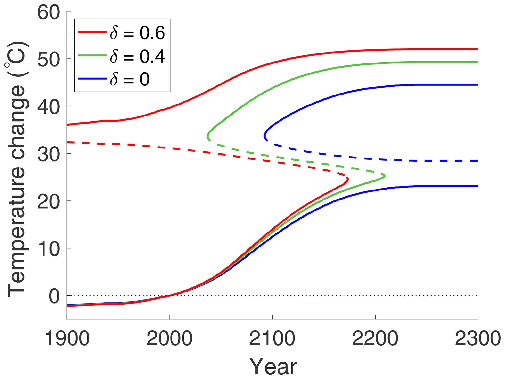
Figure 8 Arctic surface temperature change with increasing relative humidity of water vapour, δ=0.0, 0.4, 0.6, and with fixed F_O and F_A, projected to year 2300. (Temperature change is relative to the year 2000 temperature; see text for details.) On all three curves, CO₂ is increasing in time according to RCP 8.5. The red curve is essentially the same as that shown in Fig. 6 with δ=0.6. The blue and green curves have water vapour fixed at δ=0.0 and δ=0.4, respectively. For temperatures significantly below freezing, water vapour makes little contribution to temperature change. However, above freezing (τ_S>1), the greenhouse warming effect of water vapour is dramatic.

3.2.4 Anthropocene Arctic EBM summary

This EBM for the Anthropocene Arctic predicts that a bifurcation will occur, leading to catastrophic warming of the Arctic if CO₂ emissions continue to increase along RCP 8.5 without mitigation. This is true in the model even if ocean and atmosphere heat transport remain unchanged. The amplifying effects of ocean and atmosphere heat transport can make this abrupt climate change become even more dramatic and occur even earlier. Water vapour feedback further intensifies global warming. However, the EBM predicts that RCPs with reduced CO₂ emissions (due, for example, to effective mitigation strategies if introduced soon enough) may avert the drastic consequences of such a bifurcation.

Further work on Anthropocene Arctic climate modelling will include the effects of other positive feedback mechanisms, e.g. the greenhouse effects of methane and CO₂ that will be released as the permafrost thaws in the Arctic and the Hadley cell feedback that may occur as global circulation patterns change. With such additional amplification in the Arctic taken into account, and no mitigation strategies in place, a saddle-node bifurcation resulting in a transition to a warmer Arctic climate state may occur even earlier than predicted by the present model.

3.3 EBM for the Anthropocene Antarctic

It has long been recognized that the climate of the Southern Hemisphere is generally colder than that of the Northern Hemisphere for a number of reasons (Feulner et al., 2013). In particular the Antarctic is colder than the Arctic. The Antarctic climate is affected by the Antarctic Circumpolar Current (ACC), which flows freely west to east around Antarctica in the Southern Ocean, unimpeded by continental barriers. The ACC blocks the poleward heat transport from the warm oceans of the Southern Hemisphere (Hartmann, 2016). Hence, F_O is restricted to be below 20 W m⁻² in the Antarctic EBM. Additionally, the cold surface albedo α_C=0.8 is greater for the Antarctic than the Arctic, because the snow and ice that covers the continent is more pure than that in the Arctic. Cloud albedo is reduced, with a value of 7 % as opposed to the value of 12.12 % for the Arctic (Pirazzini, 2004). Atmospheric heat transport is F_A=97 W m⁻², as determined in Zhang and Rossow (1997). Finally, the Antarctic region is much drier than the Arctic; hence, a relative humidity of δ=0.4 is used.

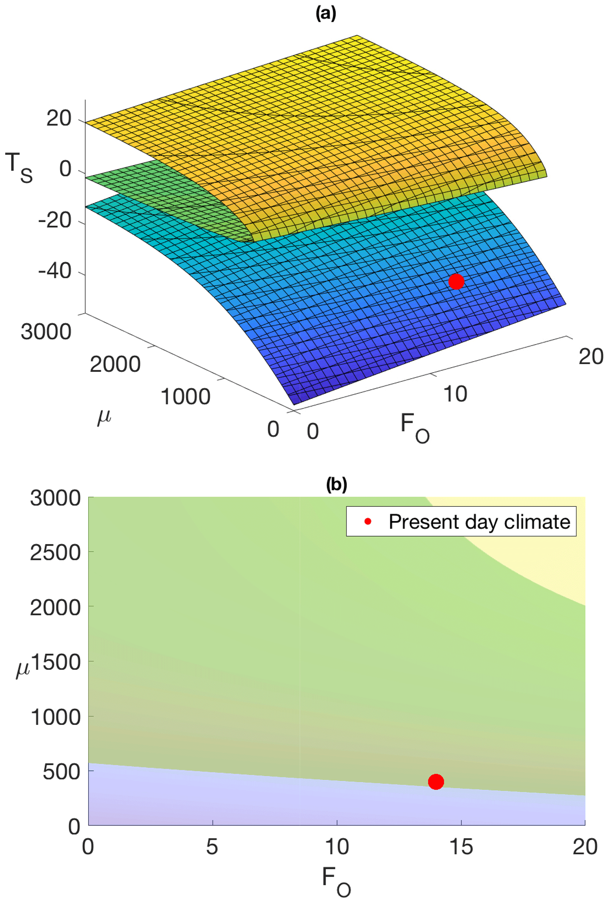
Figure 9 Energy balance model for the Antarctic. (a) 3-D equilibrium manifold, (b) Projection of the fold bifurcations. The red dot locates today's climate conditions on the cold surface.

For the Antarctic, Fig. 9a is the equilibrium manifold for the energy balance model parameterized by (F_O,μ), and Fig. 9b is the projection of the fold bifurcations onto the parameter plane. In Fig. 9b, the yellow area represents a warm stable climate, the blue area a cold stable climate, and the green area represents the overlap region (between the two fold bifurcations) where bistability exists. It can be seen in Fig. 9 that a bifurcation from a cold state to a warm state in the EBM cannot occur for an ocean heat transport value of less than F_O=12 W m⁻² and a carbon dioxide concentration less than μ=3000 ppm.

Figure 10a shows the temperature change, following each of the RCP curves in the Antarctic, extended to the year 2300. The reference temperature is $-\mathrm{32.78}{}^{\circ }\mathrm{C}$ for the year 2000, and the value of ocean heat transport into the Antarctic is assumed to be F_O=14 W m⁻², an annual mean for the sea-ice zone (approximately 70^∘S) of the Antarctic, as determined in Wu et al. (2001). This scenario does not exhibit a bifurcation from a cold climate state to a warm state. This suggests that for the Antarctic, a change in μ alone is not sufficient to cause a hysteresis loop to exist, between two coexisting stable states, in the context of modern and near-future carbon dioxide concentrations.

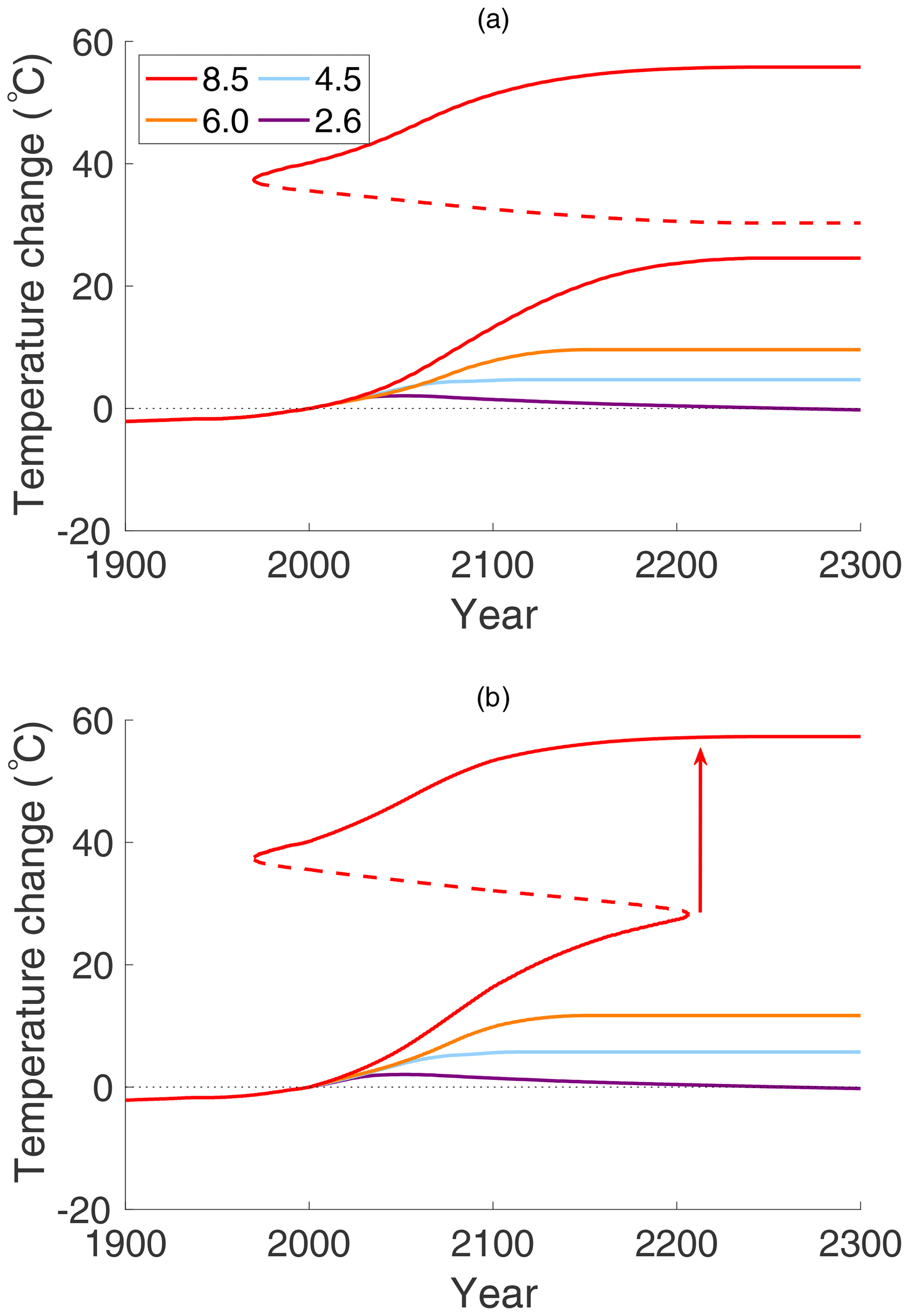
Figure 10 Antarctic surface temperature change projected to year 2300, relative to year 2000 temperature of $-\mathrm{32.78}{}^{\circ }\mathrm{C}$; (a) on each of the four RCPs with constant F_O=14 W m⁻² and (b) with increasing ocean heat transport F_O; see text for details. The upward arrow indicates the transition to a warmer equilibrium climate state after the saddle-node bifurcation.

Figure 10b presents the Antarctic model for values of F_O that increase with time as μ increases. The value of F_O is kept constant at 5 W m⁻² until the year 2000, after which time it increases linearly up to the year 2100, where it has a value of F_O=20 W m⁻², after which it is held constant again. This increase might represent an increase in sea levels, caused by thawing of the Arctic, loss of the Antarctic ice shelves, and subsequent increase in ocean heat transport (Koenigk and Brodeau, 2014). The first thing to notice is that a hysteresis loop now exists. With increasing CO₂ on RCP 8.5, there is a jump between stable states, from $\mathrm{\Delta }T=+\mathrm{29.1}{}^{\circ }\mathrm{C}$ to $\mathrm{\Delta }T=+\mathrm{56.5}{}^{\circ }\mathrm{C}$, occurring in year 2225, where ΔT is the change in surface temperature relative to the year 2000 temperature of $-\mathrm{32.78}{}^{\circ }\mathrm{C}$. The above-freezing average temperatures on the upper warm branch of equilibrium states are consistent with estimates of Antarctic temperatures in the Eocene (Passchier et al., 2013). Such a transition would imply melting of the Antarctic ice cap and a drastic rise in sea levels around the world. The return bifurcation from warm to cold (with time reversed) is visible in Fig. 10b. The “cold-to-warm” transition occurs at a later time in the Antarctic than in the Arctic and at a higher temperature. The differences between the Antarctic and Arctic bifurcations in the EBM are due to the differences in ocean heat transport and ice albedos. The difference could be larger if other factors are taken into account, e.g. the Antarctic has thicker ice and hence more heat is required to melt enough ice to cause a change in albedo. This could be represented with a larger value of ω in the tanh switch function; then, a greater temperature change is required for the function to switch from a cold albedo value to a warm one.

3.4 EBM for the Anthropocene tropics

Next, the EBM is adapted to model the climate of the tropics by choosing parameter values that are annual mean, zonally averaged values at the Equator. This gives insolation Q=418.8 W m⁻² and relative humidity δ=0.8. Heat transports $F_{\mathrm{A}}=-\mathrm{38}$ W m⁻² and $F_{\mathrm{O}}=-\mathrm{39}$ W m⁻² are both negative, because heat is transported away from the Equator towards the poles (Hartmann, 2016). The shortwave cloud cooling ξ_R (the albedo of the clouds) is also greater in the tropics, and the surface has a lower albedo. The value ξ_R=22.35 % is determined in the appendix from the global energy budgets of Trenberth et al. (2009) and Wild et al. (2013).

As the tropics have annual average temperatures well above the freezing point of water, ice–albedo feedback is absent in the tropics and a bifurcation from a cold stable state to a warm state can not occur under Anthropocene conditions. However, if forced to low F_O, F_A values and very low carbon dioxide levels, the climate state known as “snowball Earth” (Kaper and Engler, 2013; Pierrehumbert, 2010) is a possibility. That scenario is not explored in this paper, as it is not relevant to the Anthropocene.

The large relative humidity of δ=0.8 in the tropics serves to mitigate the radiative forcing of increasing CO₂. Water vapour is a much more effective greenhouse gas than carbon dioxide (Pierrehumbert, 2010). The atmosphere of the tropics contains more water vapour (the product of greater relative humidity and warmer temperatures). The total atmospheric longwave absorption η is given in Eq. (9). In the EBM of the tropics, the water vapour content is so high that η_W (and thus total absorptivity η) is almost “maxed out” at η≈1. Hence the total absorptivity is dominated by the contribution due to water vapour, and an increase in CO₂ concentration has little additional greenhouse warming effect.

Figure 11 reveals relatively low increases in temperature for the tropics compared to the poles, as CO₂ concentration increases along the RCPs. Both the absence of a bifurcation and the mitigation due to a large existing water vapour greenhouse forcing taken together cause the temperature increase relative to the year 2000 to be less than 2^∘C, in all four RCP scenarios.

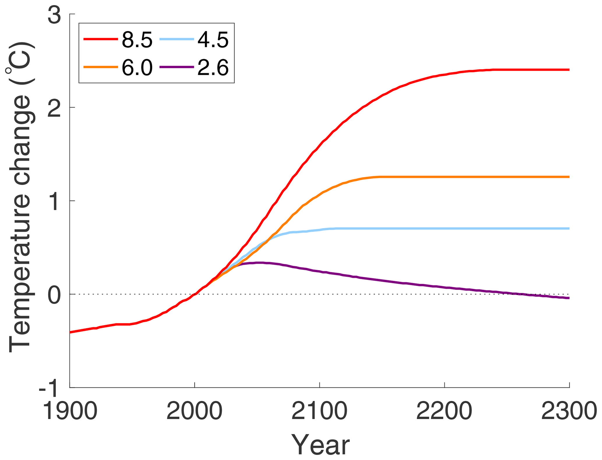
Figure 11 Tropical surface temperature changes for the four RCP scenarios, forecast to year 2300 relative to year 2000 (25.19 ^∘C), with constant F_O and F_A. The temperature change is relatively small in the tropics.

3.5 EBM for globally averaged temperature

Changes in globally averaged temperature can be modelled more easily than changes in regional temperatures due to the fact that, in a globally averaged equilibrium model, overall net horizontal transport of energy, by the oceans and the atmosphere, are both zero. Thus, the two-layer EBM Eqs. (4) and (5), globally averaged with F_O=0 and F_A=0, are simplified as follows.

$$\begin{array}{}\text{(19a)}& {\displaystyle \frac{\mathrm{d}{\mathit{\tau }}_{\mathrm{S}}}{\mathrm{d}\widehat{s}}}& {\displaystyle }=(\mathrm{1}-\mathit{\alpha })(\mathrm{1}-{\mathit{\xi }}_{\mathrm{A}}-{\mathit{\xi }}_{\mathrm{R}})q-f_{\mathrm{C}}+\mathit{\beta }{i}_{\mathrm{A}}-{\mathit{\tau }}_{\mathrm{S}}^{\mathrm{4}},\text{(19b)}& {\displaystyle \frac{\mathrm{d}{i}_{\mathrm{A}}}{\mathrm{d}\widehat{s}}}& {\displaystyle }=\mathit{\chi }[f_{\mathrm{C}}+q{\mathit{\xi }}_{\mathrm{A}}+\mathit{\eta }{\mathit{\tau }}_s^{\mathrm{4}}-i_{\mathrm{A}}].\end{array}$$

Here α is as defined in Eq. (8), η is as in Eq. (9), and f_C is as in Eq. (10). Parameters ξ_A and ξ_R are as in Table 1 and Sect. 2.1.

Figure 12 shows the change in globally averaged equilibrium surface temperature relative to the year 2000 global average (τ_S=1.064, 17.59 ^∘C), as determined by the EBM Eq. (19) to the year 2300. It is assumed that CO₂ evolves with time along each of the four RCPs defined in IPCC (2013) and displayed in Fig. 4. The other parameters, assumed constant, are as follows. The global relative humidity δ is fixed at a value of 0.74. This is determined from Dai (2006), where it lies at the lower end of a range of averages. Surface albedo is highly variable regionally, so a global average was calculated from Wild et al. (2013), much like the atmospheric shortwave absorption and the cloud albedo. From Fig. 1 of Wild et al. (2013), of the global average solar radiation of 185 W m⁻² that reaches the surface, a portion of 24 W m⁻² is reflected. Thus, the global average surface albedo is $\frac{\mathrm{24}}{\mathrm{185}}=\mathrm{0.13}=\mathrm{13}\mathit{\%}$. The values for cloud albedo and atmospheric shortwave radiation are calculated as follows. The global average incident solar radiation Q at the top of the atmosphere is 340 W m⁻², of which $\frac{\mathrm{100}-\mathrm{24}}{\mathrm{340}}=\mathrm{0.2235}=\mathrm{22.35}\mathit{\%}$ is reflected by clouds and $\frac{\mathrm{79}}{\mathrm{340}}=\mathrm{0.2324}=\mathrm{23.24}\mathit{\%}$ is absorbed by the atmosphere. The planetary boundary layer (PBL) altitude is 600 m (Ganeshan and Wu, 2016). Finally, for the purposes of sensible and latent heat transport (see appendix), the wind speed U is 5 m s⁻¹ (Nugent et al., 2014) and the drag coefficient is $C_{\mathrm{D}}=\mathrm{1.5}\times {\mathrm{10}}^{-\mathrm{3}}$.

Figure 12 Change in globally averaged surface temperature, relative to year 2000 global average temperature of 17.59 ^∘C, calculated to the year 2300 for the EBM on each of the four RCPs.

3.6 Equilibrium climate sensitivity

Equilibrium climate sensitivity (ECS) is a useful and widely adopted tool used to estimate the effects of anthropogenic forcing in a given climate model. The ECS of a model is defined as the change in the globally averaged surface temperature, after equilibrium is obtained, in response to a doubling of atmospheric CO₂ levels (IPCC, 2013; Knutti et al., 2017; Priostosescu and Huybers, 2017). The starting carbon dioxide concentration is that of the preindustrial climate, taken to be μ=270 ppm. The doubled value is then μ=540 ppm. Since the Earth has not yet experienced a doubling of CO₂ concentration since the industrial revolution, these numbers cannot be verified. Calculation of the global ECS for the EBM of this paper facilitates comparisons with other climate models as reported in IPCC (2013).

3.6.1 ECS for the globally averaged EBM

Table 3 gives both the nondimensional τ_S and the degree Celsius temperature values for the μ=270 climate, the μ=540 climate, and the temperature difference. This difference is the ECS of the global EBM of this paper.

Table 3 ECS for the globally averaged EBM.

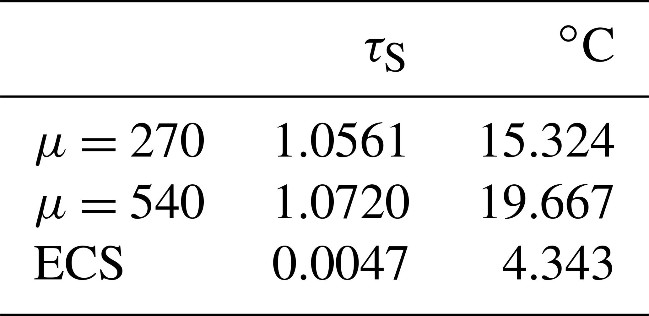
For the models used in IPCC (2013), ECS values lie within a likely range of 1.5 to 4.5 ^∘C. Values of less than 1 ^∘C are deemed to be extremely unlikely, and values greater than 6 ^∘C are very unlikely (IPCC, 2013). The value of 4.343 ^∘C calculated for this global EBM lies just inside the likely range, at the high end. Recent work gives evidence that statistical climate models based on historical data tend to lie on the lower end of likely ECS values, with a range of 1.5 to 3 ^∘C, whereas nonlinear GCMs tend to have larger ECS values (Priostosescu and Huybers, 2017). Therefore, as the global EBM presented in this paper is nonlinear and is based on physical rather than statistical modelling, it may be expected to fall on the side of larger ECS values.

3.6.2 Regional ECS values

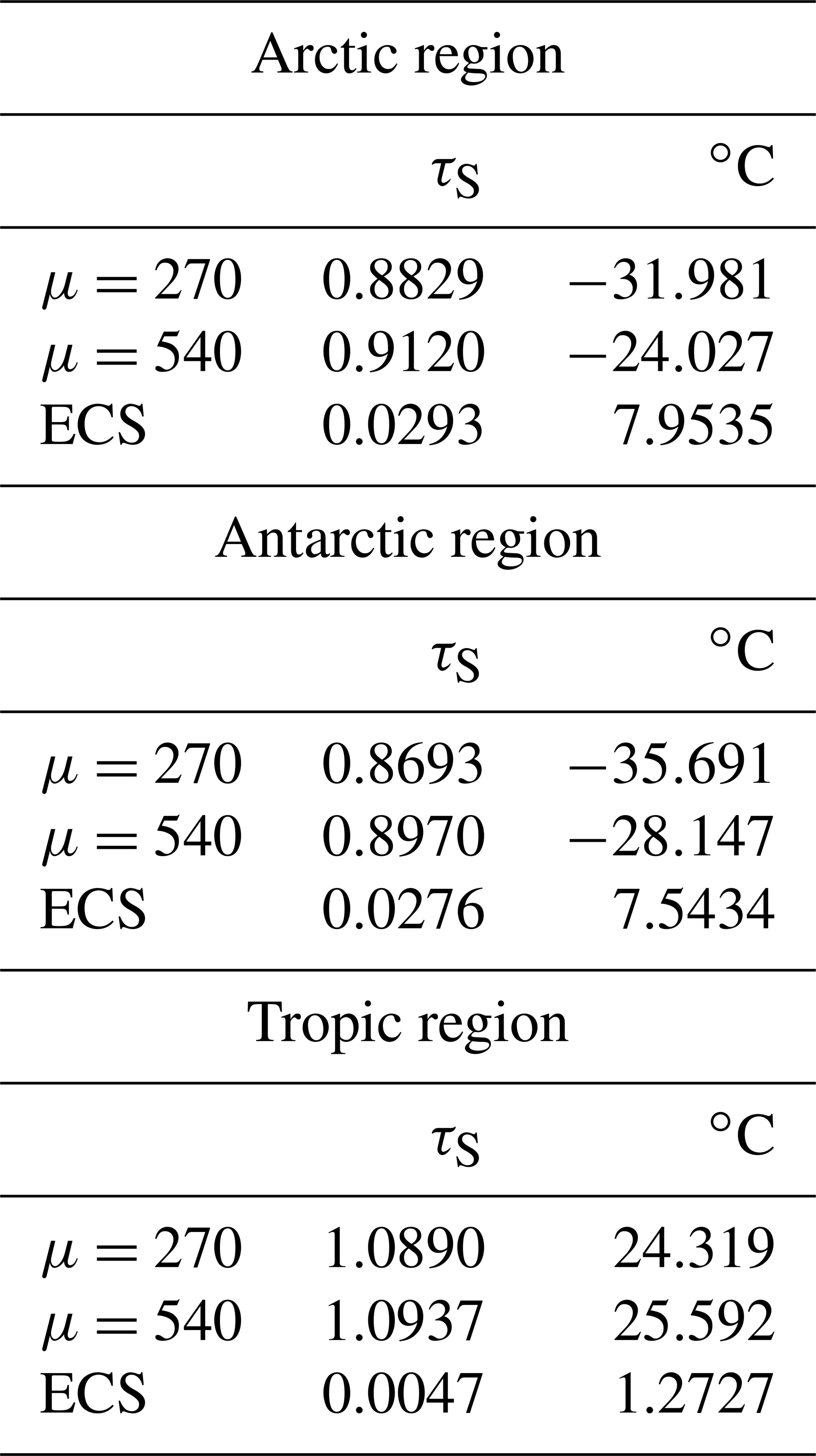
Local ECS values may be determined for each of the three regional models, the Arctic, Antarctic, and the tropics, as defined in Sects. 3.2 to 3.4. These values are given in Table 4. In all cases, F_O values are kept constant at their minimal values: 10 W m⁻² for the Arctic, 14 W m⁻² for the Antarctic, and −39 W m⁻², for the tropics. The regional ECS values are high, 7.95 and 7.54  ^∘C, respectively, for the Arctic and Antarctic, and low, 1.27  ^∘C for the tropics. Although the Earth has not yet experienced a doubling of CO₂ concentrations since the industrial revolution, these ECS values are consistent with observations to date.

Table 4 ECS values for each of the three regional EBMs. The ECS is much greater for the poles than for the tropics, in agreement with observations.

4 Conclusions and future work

The analysis of this paper shows that a cusp bifurcation can occur in an energy balance model (EBM), which could lead to hysteresis behaviour and an abrupt warming of the Anthropocene climate, to a climate state that is like nothing that has existed on Earth since the Pliocene. The model has been constructed from fundamental nonlinear processes of atmospheric physics. This bifurcation is most likely to occur in the Arctic climate. It would lead to catastrophic warming, if increases in atmospheric CO₂ continue on their current pathway. However, if the increase in atmospheric CO₂ is mitigated sufficiently, this bifurcation can still be avoided. Climate changes in the Arctic, Antarctic, and tropics are compared. The globally averaged equilibrium climate sensitivity (ECS) of the EBM is 4.34 ^∘C, which is at the high end of the likely range reported in IPCC (2013).

Future work will strengthen the conclusions of this paper by extending this simple EBM to more comprehensive models, which still allow rigorous bifurcation analysis to be performed. In the first generalization, the two-layer model will be replaced with a column model, with the atmosphere extending continuously from the surface to the tropopause. The ICAO Standard Atmosphere assumption will be replaced with a Schwarzschild radiation model of the atmosphere (Pierrehumbert, 2010), which will determine the lapse rate from the solution of a two-point boundary value problem. This Schwarzschild column model will be used to study, in addition to the positive feedback processes of this paper, the amplifying effects of methane from permafrost feedback in the Arctic.

The next generalization will combine the ideas of these energy balance models with a 3-D Navier–Stokes–Boussinesq partial differential equation (PDE) model, representing the convectively driven atmosphere as a fluid in a rotating spherical shell, presented in Lewis and Langford (2008) and Langford and Lewis (2009). In that model, surface temperatures were prescribed as boundary conditions; however, with the assumption of an energy balance constraint, the meridional surface temperature gradient will be determined implicitly. Meridional heat transport also will be determined in this model and may be compared with the poleward heat transports in the EBM of this paper. The code to solve this PDE model for a cusp bifurcation has been written. Later, guided by these results, the climate bifurcations found in these analytical models will be sought in an open-source general circulation model. This hierarchy of models is expected to add credibility to the prediction, presented here, that the Earth's climate system is capable of exhibiting dramatic topological changes (bifurcations) in the Anthropocene, leading to a climate state that resembles the pre-Pliocene climate of Earth.

Appendix A: Determination of parameters in the Anthropocene EBM

The determination of the physical parameters appearing in the EBM (Eqs. 4 and 5) is summarized here. In most cases, these parameters were determined in earlier papers of the authors dealing with paleoclimates (Dortmans et al., 2019; Kypke and Langford, 2020). The focal point is the scaled, two-dimensional Eqs. (4) and (5) in Sect. 2.1, with α given by Eq. (8), η given by Eq. (9), and f_C given by Eq. (10).

First consider the incoming solar radiation Q. A fraction ξ_A is absorbed by the atmosphere and a fraction ξ_R is reflected by the clouds, as seen in Fig. 1 and Eqs. (4) and (5). These fractions were determined in Kypke (2019) and appendix A1 of Dortmans et al. (2019), using data for the global average energy budget described in Trenberth et al. (2009), Wild et al. (2013); and Kim and Ramanathan (2012). The globally averaged values were ξ_A=0.2324 and ξ_R=0.2235 as listed in Table 1. For the polar regions, the albedo of clouds is less than elsewhere. Using data collected in the Surface Heat Budget of the Arctic Ocean (SHEBA) program (Intrieri et al,, 2002; Shupe and Intrieri, 2003), the revised polar value of ξ_R=0.1212 was determined in Kypke (2019).

Clouds in the atmosphere have a second main effect, the absorption of a fraction, η_Cl, of the longwave radiation outgoing from the surface of the Earth (Hartmann, 2016). This effect warms the Earth's atmosphere. Through data in the SHEBA program, the longwave cloud forcing in the Arctic was found to be 51 W m⁻² in the paper of Shupe and Intrieri (2003). Using this SHEBA data, Kypke (2019) determined the fraction η_Cl=0.255, as used in Eq. (9); see Table 1.

The absorption coefficients k_C for carbon dioxide and k_W for water vapour in the atmosphere (see Table 1) were calculated using an empirical approach, based on the modern-day global energy budget (Trenberth et al., 2009; Wild et al., 2013). Figure 1 in Trenberth et al. (2009) provides the global mean surface radiation as 396 W m⁻², along with an atmospheric window of 40 W m⁻². This atmospheric window, $\frac{\mathrm{40}}{\mathrm{396}}\approx \mathrm{0.1}$, is then equal to 1−η. Schmidt et al. (2010) provide percentage contributions of carbon dioxide and water vapour and clouds in an all-sky scenario, based on simulations using modern climate conditions from the year 1980. The calculated values for η_C and η_W are then used to calculate the corresponding optical depths, λ_C, and λ_W for the case of the modern atmosphere, and these are used to solve for k_C and k_W, which then appear in the G_C and G_W2 terms, respectively, in Table 1 and Eq. (7).

The vertical transport of sensible and latent heat is a difficult and complicated process to model, so many approximations are made to keep it within the scope of this work. For more details, see Kypke (2019). The heat transports are modelled via bulk aerodynamic exchange formulae describing fluxes between the surface and the atmosphere (Pierrehumbert, 2010; Hartmann, 2016). For the sensible heat flux, c_p is the specific heat of the air being heated, and T is its temperature. The bulk aerodynamic formula for sensible heat (SH) is

$$\begin{array}{}\text{(A1)}& \text{SH}=c_{\mathrm{p}}\mathit{\rho }{C}_{\text{DS}}U(T_{\mathrm{S}}-T_{\mathrm{A}}),\end{array}$$

where C_DS is the drag coefficient for temperature and U is the mean horizontal wind velocity. The density of the atmosphere ρ is determined as a function of both surface temperature T_S and altitude Z using the barometric formula, and a constant lapse rate Γ (ICAO, 1993) is used to determine the temperature gradient.

In the case of latent heat (LH), the moisture content is represented by L_vr, where L_v is the latent heat of vaporization of water and r is the mass mixing ratio of condensable air to dry air (Pierrehumbert, 2010). Then

$$\begin{array}{}\text{(A2)}& \text{LH}=L_{\mathrm{v}}\mathit{\rho }{C}_{\text{DL}}U(r_{\mathrm{S}}-r_{\mathrm{A}}),\end{array}$$

where C_DL is the drag coefficient for moisture. In the following, for simplicity, we set

$${\displaystyle }{\displaystyle }{C}_{\text{DS}}=C_{\text{DL}}\equiv C_{\mathrm{D}}.$$

The mass mixing ratio is equal to the saturation mixing ratio times the relative humidity. The saturation mixing ratio depends on the saturation vapour pressure, which is a function of temperature as given by the Clausius–Clapeyron Eq. (6). The sensible and latent heat transports are combined into a single term, F_C, which replaces the F_C term that was introduced in Dortmans et al. (2019). This term is defined here as a function of surface temperature T_S.

$$\begin{array}{ll}{\displaystyle }{F}_{\mathrm{C}}\left(T_{\mathrm{S}}\right)=& {\displaystyle \frac{C_{D}U}{(T_{\mathrm{S}}-\mathrm{\Gamma }Z)}}[{\displaystyle \frac{c_{\mathrm{p}}{P}_{\mathrm{0}}\mathrm{\Gamma }Z}{R_{\mathrm{A}}}}+{\displaystyle \frac{L_{\mathrm{v}}{P}^{\text{sat}}\left(T_{\mathrm{R}}\right)}{R_{\mathrm{w}}}}\\ \text{(A3)}& {\displaystyle }& {\displaystyle }(e^{\left[G_{\text{W1}}\frac{T_{\mathrm{S}}-T_{\mathrm{R}}}{T_{\mathrm{S}}}\right]}-\mathit{\delta }{e}^{\left[G_{\text{W1}}\frac{T_{\mathrm{S}}-\mathrm{\Gamma }Z-T_{\mathrm{R}}}{T_{\mathrm{S}}-\mathrm{\Gamma }Z}\right]})]\end{array}$$

Here, P₀ is the atmospheric pressure at the surface (Z=0) and R_A is the ideal gas constant specific to dry air. This equation is scaled by $\frac{\mathrm{1}}{\mathit{\sigma }{T}_{\mathrm{R}}^{\mathrm{4}}}$ to nondimensionalize it, creating $f_{\mathrm{C}}=\frac{F_{\mathrm{C}}}{\mathit{\sigma }{T}_{\mathrm{R}}^{\mathrm{4}}}$ in Eq. (10), where T_R=273.15 K is the reference temperature. As this f_C represents energy moving from the surface to the atmosphere, it is subtracted from the surface Eq. (4) and added to the atmosphere Eq. (5). A different model of F_C, used by the authors in Dortmans et al. (2019), was a simple functional form calibrated to empirical data. The result was a relationship between F_C and T_S that is quantitatively very similar to that given by Eq. (A3). In Kypke and Langford (2020), F_C was set equal to zero for the paleoclimate Arctic and Antarctic models for simplicity, since both SH and LH are very small for temperatures that are below freezing.