Data-driven predictions of a multiscale Lorenz 96 chaotic system using machine-learning methods: reservoir computing, artificial neural network, and long short-term memory network

In this paper, the performance of three machine-learning methods for predicting short-term evolution and for reproducing the long-term statistics of a multiscale spatiotemporal Lorenz 96 system is examined. The methods are an echo state network (ESN, which is a type of reservoir computing; hereafter RC–ESN), a deep feed-forward artificial neural network (ANN), and a recurrent neural network (RNN) with long short-term memory (LSTM; hereafter RNN–LSTM). This Lorenz 96 system has three tiers of nonlinearly interacting variables representing slow/large-scale (X), intermediate (Y), and fast/small-scale (Z) processes. For training or testing, only X is available; Y and Z are never known or used. We show that RC–ESN substantially outperforms ANN and RNN–LSTM for short-term predictions, e.g., accurately forecasting the chaotic trajectories for hundreds of numerical solver's time steps equivalent to several Lyapunov timescales. The RNN–LSTM outperforms ANN, and both methods show some prediction skills too. Furthermore, even after losing the trajectory, data predicted by RC–ESN and RNN–LSTM have probability density functions (pdf's) that closely match the true pdf – even at the tails. The pdf of the data predicted using ANN, however, deviates from the true pdf. Implications, caveats, and applications to data-driven and data-assisted surrogate modeling of complex nonlinear dynamical systems, such as weather and climate, are discussed.

1 Introduction

Various components of the Earth system involve multiscale, multiphysics processes and high-dimensional chaotic dynamics. These processes are often modeled using sets of strongly coupled nonlinear partial differential equations (PDEs), which are solved numerically on supercomputers. As we aim to simulate such systems with increasing levels of fidelity, we need to increase the numerical resolutions and/or incorporate more physical processes from a wide range of spatiotemporal scales into the models. For example, in atmospheric modeling for predicting the weather and climate systems, we need to account for the nonlinear interactions across the scales of cloud microphysics processes, gravity waves, convection, baroclinic waves, synoptic eddies, and large-scale circulation, just to name a few (not to mention the fast/slow processes involved in feedbacks from the ocean, land, and cryosphere; Collins et al., 2006, 2011; Flato, 2011; Bauer et al., 2015; Jeevanjee et al., 2017).

Solving the coupled systems of PDEs representing such multiscale processes is computationally highly challenging for many practical applications. As a result, to make the simulations feasible, a few strategies have been developed, which mainly involve only solving for slow/large-scale variables and accounting for the fast/small-scale processes through surrogate models. In weather and climate models, for example, semiempirical physics-based parameterizations are often used to represent the effects of processes such as gravity waves and moist convection in the atmosphere or submesoscale eddies in the ocean (Stevens and Bony, 2013; Hourdin et al., 2017; Garcia et al., 2017; Jeevanjee et al., 2017; Schneider et al., 2017b; Chattopadhyay et al., 2020b, a). A more advanced approach is “super-parameterization” which, for example, involves solving the PDEs of moist convection on a high-resolution grid inside each grid point of large-scale atmospheric circulation for which the governing PDEs (the Navier–Stokes equations) are solved on a coarse grid (Khairoutdinov and Randall, 2001). While computationally more expensive, super-parameterized climate models have been shown to outperform parameterized models in simulating some aspects of climate variability and extremes (Benedict and Randall, 2009; Andersen and Kuang, 2012; Kooperman et al., 2018).

More recently, “inexact computing” has received attention from the weather and climate community. This approach involves reducing the computational cost of each simulation by decreasing the precision of some of the less-critical calculations (Palem, 2014; Palmer, 2014), thus allowing the saved resources to be reinvested, for example, in more simulations (e.g., for probabilistic predictions) and/or higher resolutions for critical processes (Düben et al., 2014; Düben and Palmer, 2014; Thornes et al., 2017; Hatfield et al., 2018). One type of inexact computing involves solving the PDEs of some of the processes with single- or half-precision arithmetic, which requires less computing power and memory compared to the conventional double-precision calculations (Palem, 2014; Düben et al., 2015; Leyffer et al., 2016).

In the past few years, the rapid algorithmic advances in machine learning (ML) and in particular data-driven modeling have been explored for improving the simulations and predictions of nonlinear dynamical systems (Schneider et al., 2017a; Kutz, 2017; Gentine et al., 2018; Moosavi et al., 2018; Wu et al., 2019; Toms et al., 2019; Brunton and Kutz, 2019; Duraisamy et al., 2019; Reichstein et al., 2019; Lim et al., 2019; Scher and Messori, 2019; Chattopadhyay et al., 2020c). One appeal of the data-driven approach is that fast and accurate data-driven surrogate models that are trained on data of high fidelity can be used to accelerate and/or improve the predictions and simulations of complex dynamical systems. Furthermore, for some poorly understood processes for which observational data are available (e.g., clouds), data-driven surrogate models built using such data might potentially outperform physics-based surrogate models (Schneider et al., 2017a; Reichstein et al., 2019). Recent studies have shown promising results in using ML to build data-driven parameterizations for the modeling of some atmospheric and oceanic processes (Rasp et al., 2018; Brenowitz and Bretherton, 2018; Gagne et al., 2020; O'Gorman and Dwyer, 2018; Bolton and Zanna, 2019; Dueben and Bauer, 2018; Watson, 2019; Salehipour and Peltier, 2019). In the turbulence and dynamical systems communities, similarly encouraging outcomes have been reported (Ling et al., 2016; McDermott and Wikle, 2017; Pathak et al., 2018a; Rudy et al., 2018; Vlachas et al., 2018; Mohan et al., 2019; Wu et al., 2019; Raissi et al., 2019; Zhu et al., 2019; McDermott and Wikle, 2019).

The objective of the current study is to make progress toward addressing the following question: which AI-based data-driven technique(s) can best predict the spatiotemporal evolution of a multiscale chaotic system, when only the slow/large-scale variables are known (during training) and are of interest (to predict during testing)? We emphasize that, unlike many other studies, our focus is not on reproducing long-term statistics of the underlying dynamical system (although that will be examined too) but on predicting the short-term trajectory from a given initial condition. Furthermore, we emphasize that, following the problem formulation introduced by Dueben and Bauer (2018), the system's state vector is only partially known and the fast/small-scale variables are unknown even during training.

Our objective is more clearly demonstrated using the canonical chaotic system that we will use as a test bed for the data-driven methods, a multiscale Lorenz 96 system, as follows:

$$\begin{array}{ll}\text{(1)}& {\displaystyle \frac{\mathrm{d}{X}_k}{\mathrm{d}t}}=& {\displaystyle }{X}_{k-\mathrm{1}}\left(X_{k+\mathrm{1}}-X_{k-\mathrm{2}}\right)+F-{\displaystyle \frac{hc}{b}}{\mathrm{\Sigma }}_j{Y}_{j,k},{\displaystyle \frac{\mathrm{d}{Y}_{j,k}}{\mathrm{d}t}}=& {\displaystyle }-cb{Y}_{j+\mathrm{1},k}\left(Y_{j+\mathrm{2},k}-Y_{j-\mathrm{1},k}\right)-c{Y}_{j,k}+{\displaystyle \frac{hc}{b}}{X}_k\\ \text{(2)}& {\displaystyle }& {\displaystyle }-{\displaystyle \frac{he}{d}}{\mathrm{\Sigma }}_i{Z}_{i,j,k},{\displaystyle \frac{\mathrm{d}{Z}_{i,j,k}}{\mathrm{d}t}}=& {\displaystyle }ed{Z}_{i-\mathrm{1},j,k}\left(Z_{i+\mathrm{1},j,k}-Z_{i-\mathrm{2},j,k}\right)-ge{Z}_{i,j,k}\\ \text{(3)}& {\displaystyle }& {\displaystyle }+{\displaystyle \frac{he}{d}}{Y}_{j,k}.\end{array}$$

This set of coupled nonlinear ordinary differential equations (ODEs) is a three-tier extension of Lorenz's original model (Lorenz, 1996) and has been proposed by Thornes et al. (2017) as a fitting prototype for multiscale chaotic variability of the weather and climate system and a useful test bed for novel methods. In these equations, F=20 is a large-scale forcing that makes the system highly chaotic, and $b=c=e=d=g=\mathrm{10}$ and h=1 are tuned to produce appropriate spatiotemporal variability of the three variables (see below). The indices are $i,j,k=\mathrm{1},\mathrm{2},\mathrm{\dots }\mathrm{8}$; thus X has 8 elements while Y and Z have 64 and 512 elements, respectively. Figure 1 shows examples of the chaotic temporal evolution of X, Y, and Z obtained from directly solving Eqs. (1)–(3). The examples demonstrate that X has large amplitudes and slow variability; Y has relatively small amplitudes, high-frequency variability, and intermittency; and Z has small amplitudes and high-frequency variability. In the context of atmospheric circulation, the slow variable X can represent the low-frequency variability of the large-scale circulation, while the intermediate variable Y and fast variable Z can represent synoptic and baroclinic eddies and small-scale convection, respectively. Similar analogies in the context of ocean circulation and various other natural or engineering systems can be found, making this multiscale Lorenz 96 system a useful prototype to focus on.

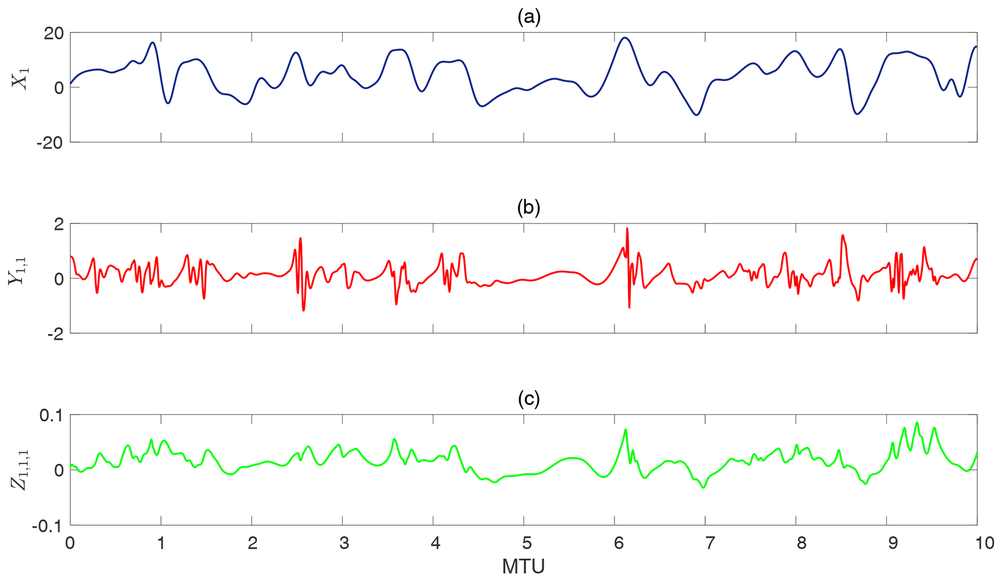
Figure 1 Time evolution of (a) X_k at grid point k=1, (b) Y_j,1 at grid point j=1, and (c) $Z_{i,\mathrm{1},\mathrm{1}}$ at grid point i=1. The time series show chaotic behavior in X, which has large amplitude and slow variability; Y, which has relatively small amplitudes, high-frequency variability, and intermittency; and Z, which has small amplitudes and high-frequency variability. The x axis is in model time units (MTUs), which are related to the time step of the numerical solver (Δt) and largest positive Lyapunov exponent (λ_max) as $\mathrm{1}\mathrm{MTU}=\mathrm{200}\mathrm{\Delta }t\approx \mathrm{4.5}/{\mathit{\lambda }}_{max}$ (see Sect. 2.1). Note that here we are presenting raw data which have not been standardized for predictions or testing yet.

Our objective is to predict the spatiotemporal evolution of X(t) using a data-driven model that is trained on past observations of X(t); Fig. 2. In the conventional approach of solving Eqs. (1)–(3) numerically, the governing equations have to be known, initial conditions for Y(t) and Z(t) have to be available, and the numerical resolution is dictated by the fast/small-scale variable Z, leading to high computational costs. In the fully data-driven approach that is our objective here, the governing equations do not have to be known, Y(t) and Z(t) do not have to be observed at any time, and the evolution of X(t) is predicted just from knowledge of the past observations of X, leading to low computational costs. To successfully achieve this objective, a data-driven method should be able to do the following:

1. accurately predict the evolution of a chaotic system along a trajectory for some time

2. account for the effects of Y(t) and Z(t) on the evolution of X(t).

Inspired by several recent studies (which will be discussed below), we have focused on evaluating the performance of three ML techniques in accomplishing (1) and (2). These data-driven methods are as follows:

• RC–ESN: echo state network (ESN), a specialized type of recurrent neural network (RNN), which belongs to the family of reservoir computing (RC);

• ANN: a deep feed-forward artificial neural network; and

• RNN–LSTM: an RNN with long short-term memory (LSTM).

We have focused on these three methods because they have either shown promising performance in past studies (RC–ESN and ANN), or they are considered to be state of the art in learning from sequential data (RNN–LSTM). There are a growing number of studies focused on using machine-learning techniques for data-driven modeling of chaotic and turbulent systems, for example, to improve weather and climate modeling and predictions. Some of these studies have been referenced above. Below, we briefly describe three sets of studies with the closest relevance to our objective and approach. Pathak and coworkers (Pathak et al., 2017, 2018a; Lu et al., 2017; Fan et al., 2020) have recently shown promising results with RC–ESN for predicting short-term spatiotemporal evolution (item 1) and in replicating attractors for the Lorenz 63 and Kuramoto–Sivashinsky equations. The objective of our paper (items 1–2) and the employed multiscale Lorenz 96 system are identical to that of Dueben and Bauer (2018), who reported their ANN to have some skills in data-driven predictions of the spatiotemporal evolution of X. Finally, Vlachas et al. (2018) found an RNN–LSTM to have skills (though limited) for predicting the short-term spatiotemporal evolution (item 1) of a number of chaotic toy models such as the original Lorenz 96 system. Here we aim to build on these pioneering studies and examine, side by side, the performance of RC–ESN, ANN, and RNN–LSTM in achieving (1) and (2) for the chaotic multiscale Lorenz 96 system. We emphasize the need for a side-by-side comparison that uses the same system as the test bed and metrics for assessing performance.

The structure of the paper is as follows: in Sect. 2, the multiscale Lorenz 96 system and the three ML methods are discussed, results on how these methods predict the short-term spatiotemporal evolution of X and reproduce the long-term statistics of X are presented in Sect. 3, and key findings and future work are discussed in Sect. 4.

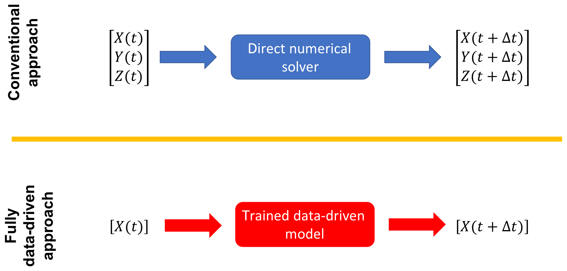
Figure 2 The conventional approach of solving the full governing equations numerically versus our data-driven approach for predicting the spatiotemporal evolution of the slow/large-scale variable X. For the direct numerical solution, the governing equations have to be known and the numerical resolution is dictated by the fast and small-scale variable Z, resulting in high computational costs. In the data-driven approach, the governing equations do not have to be known, Y and Z do not have to be known, and evolution of X is predicted just from knowing the past observations of X, leading to low computational costs.

2 Materials and methods

2.1 The multiscale Lorenz 96 system

2.1.1 Numerical solution

We have used a fourth-order Runge–Kutta solver, with time step Δt=0.005, to solve the system of Eqs. (1)–(3). The system has been integrated for 100 million time steps to generate a large dataset for training, testing, and examination of the robustness of the results. In the Results section, we often report time in terms of model time units (MTUs), where 1 MTU=200Δt. In terms of the Lyapunov timescale, 1 MTU in this system is $\approx \mathrm{4.5}/{\mathit{\lambda }}_{max}$ (Thornes et al., 2017), where λ_max is the largest positive Lyapunov exponent. In terms of the e-folding decorrelation timescale (τ) of the leading principal component (PC1) of X (Khodkar et al., 2019), we estimate 1 MTU≈6.9τ_PC1. Finally, as discussed in Thornes et al. (2017), 1 MTU in this system corresponds to ≈3.75 Earth days in the real atmosphere.

2.1.2 Training and testing datasets

To build the training and testing datasets from the numerical solution, we have sampled X∈ℜ⁸ at every Δt and then standardized the data by subtracting the mean and dividing by the standard deviation. We have constructed a training set consisting of N sequential samples and a testing set consisting of the next 2000 sequential samples from point N+1 to N+2000. We have randomly chosen 100 such training/testing sets, each of length (N+2000)Δt, starting from a random point and separated from the next training/testing set by at least 2000Δt. There is never any overlap between the training and the testing sequences in any of the 100 training/testing sets.

2.2 Reservoir computing–echo state network (RC–ESN)

2.2.1 Architecture

The RC–ESN (Jaeger and Haas, 2004; Jaeger, 2007) is an RNN that has a reservoir with D neurons, which are sparsely connected in an Erdős–Rényi graph configuration (see Fig. 3). The connectivity of the reservoir neurons is represented by the adjacency matrix A of size D×D for which the values are drawn from a uniform random distribution on the interval $\left[-\mathrm{1},\mathrm{1}\right]$. The adjacency matrix A is then normalized by its maximum eigenvalue (Λ_max) and then further multiplied with a scalar (ρ≤1) to build the $\stackrel{\mathrm{̃}}{\mathbf{A}}$ matrix. The state of the reservoir, representing the activations of its constituent neurons, is a vector r(t)∈ℜ^D. The typical reservoir size used in this study is D=5000 (but we have experimented with D as large as 20 000, as discussed later). The other two components of the RC–ESN are an input-to-reservoir layer, with a weight matrix of W_in, and a reservoir-to-output layer, with a weight matrix of W_out. The inputs for training are N sequential samples of X(t)∈ℜ⁸. At the beginning of the training phase, A and W_in are chosen randomly and are fixed; i.e., they do not change during training or testing and $\stackrel{\mathrm{̃}}{\mathbf{A}}$ is calculated. During training, only the weights of the output-to-reservoir layer (W_out) are updated.

W_out is the only trainable matrix in this network. This architecture yields a simple training process that has the following two key advantages:

• It does not suffer from the vanishing and the exploding gradient problem, which has been a major difficulty in training RNNs, especially before the advent of LSTMs (Pascanu et al., 2013).

• W_out can be computed in one shot (see below); thus this algorithm is orders of magnitude faster than the backpropagation through time (BPTT) algorithm (Goodfellow et al., 2016), which is used for training general RNNs and RNN–LSTMs (see Sect. 2.4).

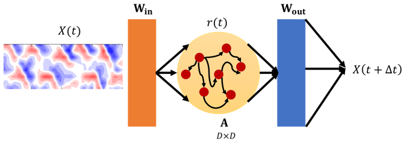
Figure 3 A schematic of RC–ESN. D×D is the size of the adjacency matrix of reservoir A. X(t) ($-T\le t\le \mathrm{0}$) is the input during training. W_in and A are random matrices that are chosen at the beginning of training and fixed during training and testing. Only W_out is computed during training. During testing (t>0), X(t+Δt) is predicted from a given X(t) that is either known from the initial condition or has been previously predicted.

The equations governing the RC–ESN training process are as follows:

$$\begin{array}{}\text{(4)}& {\displaystyle }& {\displaystyle }r(t+\mathrm{\Delta }t)=\tanh \left(\stackrel{\mathrm{̃}}{\mathbf{A}}r\left(t\right)+{\mathbf{W}}_{\text{in}}X\left(t\right)\right),\text{(5)}& {\displaystyle }& {\displaystyle }{\mathbf{W}}_{\text{out}}=\arg \underset{{\mathbf{W}}_{\text{out}}}{min}\parallel {\mathbf{W}}_{\text{out}}\stackrel{\mathrm{̃}}{r}\left(t\right)-X\left(t\right)\parallel +\mathit{\alpha }\parallel {\mathbf{W}}_{\text{out}}\parallel .\end{array}$$

Here $\parallel \cdot \parallel$ is the L₂-norm of a vector and α is the L₂ regularization (ridge regression) constant. Equation (4) maps the observable X(t)∈ℜ⁸ to the higher-dimensional reservoir's state $r(t+\mathrm{\Delta }t)\in {\mathrm{\Re }}^D$ (reminder: D is O(1000) for this problem). Note that Eq. (5) contains $\stackrel{\mathrm{̃}}{r}\left(t\right)$ rather than r(t). As observed by Pathak et al. (2018a) for the Kuramoto–Sivashinsky equation, and observed by us in this work, the columns of the matrix $\stackrel{\mathrm{̃}}{\mathbf{r}}$ should be chosen as nonlinear combinations of the columns of the reservoir state matrix r (each row of the matrix r is a snapshot r(t) of size D). For example, following Pathak et al. (2018a), we compute $\stackrel{\mathrm{̃}}{\mathbf{r}}$ as having the same even columns as r, while its odd columns are the square of the odd columns of r (algorithm T₁ hereafter). As shown in Appendix A, we have found that a nonlinear transformation (between r and $\stackrel{\mathrm{̃}}{\mathbf{r}}$) is essential for skillful predictions, while several other transformation algorithms yield similar results to T₁. The choices of these transformations (T₂ and T₃; see Appendix A), although not based on a rigorous mathematical analysis, are inspired from the nature of the quadratic nonlinearity that is present in Eqs. (1)–(3).

The prediction process is governed by the following:

$$\begin{array}{}\text{(6)}& X(t+\mathrm{\Delta }t)={\mathbf{W}}_{\text{out}}\stackrel{\mathrm{̃}}{r}(t+\mathrm{\Delta }t),\end{array}$$

where $\stackrel{\mathrm{̃}}{r}(t+\mathrm{\Delta }t)$ in Eq. (6) is computed by applying one of the T₁, T₂, or T₃ algorithms on r(t+Δt), which itself is calculated via Eq. (4) from X(t) that is either known from the initial condition or has been previously predicted.

See Jaeger and Haas (2004), Jaeger (2007), Lukoševičius and Jaeger (2009), Gauthier (2018) and references therein for further discussions on RC–ESNs, and Lu et al. (2017), Pathak et al. (2017), McDermott and Wikle (2017), Pathak et al. (2018a), Pathak et al. (2018b), Zimmermann and Parlitz (2018), Lu et al. (2018), McDermott and Wikle (2019), Lim et al. (2019) for examples of recent applications to dynamical systems.

2.2.2 Training and predictions

During training ($-T\le t\le \mathrm{0}$), W_in and A are initialized with random numbers, which stay fixed during the training (and testing) process. The state matrix r is initialized to 0. For all the experiments conducted in this study, we have empirically found that the value of ρ=0.1 yields the best results in our experiments. We have further found that in $\mathrm{0.05}\le \mathit{\rho }\le \mathrm{0.7}$ the prediction horizon of RC–ESN is not sensitive to ρ; see Appendix B. Then, the state matrix r is computed using Eq. (4) for the training set, and W_out is computed using Eq. (5). During predictions (i.e., testing) corresponding to t>0, the computed W_out is used to march forward in time (Eq. 6) while as mentioned earlier, r(t) keeps being updated using the predicted X(t); see Eq. 4. A nonlinear transformation is used to compute $\stackrel{\mathrm{̃}}{r}\left(t\right)$ from r(t) before using Eq. (6).

Our RC–ESN architecture and training/prediction procedure are similar to the ones used in Pathak et al. (2018a). There is no overfitting in the training phase because the final training and testing accuracies are the same. Our code is developed in Python and is made publicly available (see Code and data availability).

2.3 Feed-forward artificial neural network (ANN)

2.3.1 Architecture

We have developed a deep ANN that has the same architecture as the one used in Dueben and Bauer (2018) (which they employed to conduct predictions on the same multiscale Lorenz 96 studied here). The ANN has four hidden layers with 100 neurons each and 8 neurons in the input and output layers (Fig. 4). It should be noted that, unlike RC–ESN (and RNN–LSTM), this ANN is stateless, i.e., there is no hidden variable such as r(t) that tracks temporal evolution. Furthermore, unlike RC–ESN, for which the input and output are X(t), and X(t+Δt), following Dueben and Bauer (2018), the ANN's inputs/outputs are chosen to be pairs of X(t)^train and $\mathrm{\Delta }X(t{)}^{\text{train}}=X(t+\mathrm{\Delta }t{)}^{\text{train}}-X(t{)}^{\text{train}}$ (Fig. 4). During the prediction, using X(t)^test that is either known from the initial condition or has been previously calculated, ΔX(t)^test is predicted. X(t+Δt)^test is then computed via the Adams–Bashforth integration scheme as follows:

$$\begin{array}{}\text{(7)}& X(t+\mathrm{\Delta }t{)}^{\text{test}}=X(t{)}^{\text{test}}+{\displaystyle \frac{\mathrm{1}}{\mathrm{2}}}\left[\mathrm{3}\mathrm{\Delta }X\right(t{)}^{\text{test}}-\mathrm{\Delta }X(t-\mathrm{\Delta }t{)}^{\text{test}}].\end{array}$$

More details on the ANN architecture have been reported in Appendix C.

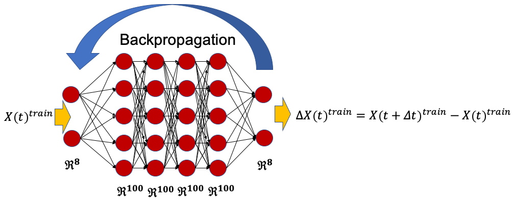
Figure 4 A schematic of ANN, which has four hidden layers each with 100 neurons and an input and an output layer each with 8 neurons (for better illustration, only a few neurons from each layer are shown). Training is performed on pairs of X(t)^train and ΔX(t)^train, and the weights in each layer are learned through the backpropagation algorithm. During testing (i.e., predictions) ΔX(t)^test is predicted for a given X(t)^test that is either known from the initial condition or that has been previously predicted. Knowing X(t)^test, ΔX(t)^test, and ΔX(t−Δt)^test, X(t+Δt)^test is then computed using the Adams–Bashforth integration scheme.

2.3.2 Training and predictions

Training is performed on N pairs of sequential (X(t)^train,ΔX(t)^train) from the training set. During training, the weights of the network are computed using backpropagation optimized by the stochastic gradient descent algorithm. During predictions, as mentioned above, ΔX(t)^test is predicted from X(t)^test that is either known from the initial condition or has been previously predicted, and X(t+Δt)^test is then calculated using Eq. (7).

Our ANN architecture and training/prediction procedure are similar to the ones used in Dueben and Bauer (2018). We have optimized, by trial and error, the hyperparameters for this particular network. There is no overfitting in the training phase because the final training and testing accuracies are the same. Our code is developed in Keras and is made publicly available (see Code and data availability).

2.4 Recurrent neural network with long short-term memory (RNN–LSTM)

2.4.1 Architecture

The RNN–LSTM (Hochreiter and Schmidhuber, 1997) is a deep-learning algorithm most suited for the predictions of sequential data, such as time series, and has received a lot of attention in recent years (Goodfellow et al., 2016). Variants of RNN–LSTMs are the best-performing models for time series modeling in areas such as stock pricing (Chen et al., 2015), supply chain (Carbonneau et al., 2008), natural language processing (Cho et al., 2014), and speech recognition (Graves et al., 2013). A major improvement over regular RNNs, which have issues with the vanishing and the exploding gradients (Pascanu et al., 2013), LSTMs have become the state-of-the-art approach for training RNNs in the deep-learning community. Unlike regular RNNs, the RNN–LSTMs have gates that control the information flow into the neural network from previous time steps of the time series. The RNN–LSTM used here, like the RC–ESN but unlike the ANN, is stateful (i.e., actively maintains its state). Our RNN–LSTM has 50 hidden layers in each RNN–LSTM cell. More details on our RNN–LSTM are presented in Appendix D. RNN–LSTMs have many tunable parameters and are trained with the expensive BPTT algorithm (Goodfellow et al., 2016).

2.4.2 Training and predictions

The input to the RNN–LSTM is a time-delay-embedded matrix of X(t) with embedding dimension q (also known as lookback; Kim et al., 1999). An extensive hyperparameter optimization (by trial and error) is performed to find the optimal value of q for which the network has the largest prediction horizon (exploring $q=\mathrm{1}-\mathrm{22}$, we found q=3 to yield the best performance). The RNN–LSTM predicts X(t+Δt) from the previous q time steps of X(t). This is in contrast with RC–ESN, which only uses X(t) and reservoir state r(t) to predict X(t+Δt), and ANN, which only uses X(t) and no state to predict X(t+Δt) (via predicting ΔX(t)). The weights of the LSTM layers are determined during the training process (see Appendix D). During testing, X(t+Δt) is predicted using the past q observables $\left[X(t-(q-\mathrm{1}\left)\mathrm{\Delta }t\right)\mathrm{\dots }X(t-\mathrm{\Delta }t),X\left(t\right)\right]$ that are either known from the initial condition or have been previously predicted. We have found the best results with a stateless LSTM (which means that the state of the LSTM is refreshed during the beginning of each batch during training; see Appendix D) that outperforms a stateful LSTM (where the states are carried over to the next batch during training).

The architecture of our RNN–LSTM is similar to the one used in Vlachas et al. (2018). There is no overfitting in the training phase because the final training and testing accuracies are the same. Our code is developed in Keras and is made publicly available (see Code and data availability).

3 Results

3.1 Short-term predictions: comparison of the RC–ESN, ANN, and RNN–LSTM performances

The short-term prediction skills of the three ML methods for the same training/testing sets are compared in Fig. 5. Given the chaotic nature of the system, the performance of the methods depends on the initial condition from which the predictions are conducted. To give the readers a comprehensive view of the performance of these methods, Fig. 5a and b shows examples of the predicted trajectories (for one element of X(t)) versus the true trajectory for two specific initial conditions (from the 100 initial conditions we used), namely the one for which RC–ESN shows the best performance (Fig. 5a), and the one for which RC–ESN shows the worst performance (Fig. 5b).

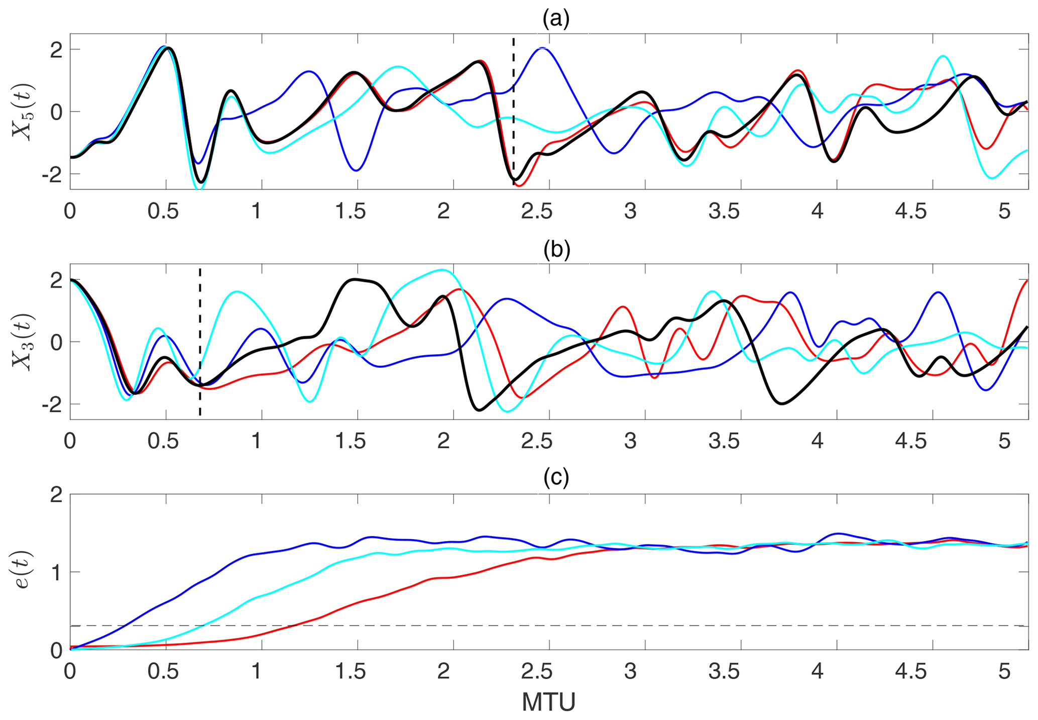
Figure 5 Comparison of the short-term forecasting skills among the three ML methods. The lines show truth (black), RC–ESN (red), ANN (blue), and RNN–LSTM (cyan). Panels (a) and (b) show examples (differing in initial condition) for which RC–ESN yields the longest and shortest prediction horizons, respectively. Vertical broken lines show the approximate prediction horizon of RC–ESN. Panel (c) shows the relative L₂ error averaged over 100 randomly chosen initial conditions e(t); see Eq. 8. The broken horizontal line marks e=0.3. Time is in MTU, where $\mathrm{1}\mathrm{MTU}=\mathrm{200}\mathrm{\Delta }t\approx \mathrm{4.5}/{\mathit{\lambda }}_{max}$. Training size is N=500 000. ρ=0.1 is used here.

For the initial condition in Fig. 5a, RC–ESN accurately predicts the time series for over 2.3 MTU, which is equivalent to 460Δt and over 10.35 Lyapunov timescales. Closer examination shows that the RC–RSN predictions follow the true trajectory well even up to ≈4 MTU. The RNN–LSTM has the next-best prediction performance (up to around 0.9 MTU or 180Δt). The predictions from ANN are around 0.6 MTU or 120Δt. For the example in Fig. 5b, all methods have shorter prediction horizons, but RC–ESN still has the best performance (accurate predictions up to ≈0.7 MTU), followed by ANN and RNN–LSTM, with similar prediction accuracies (≈0.3 MTU). Searching through all 100 initial conditions, the best predictions with RNN–LSTM are up to ≈1.7 MTU (equivalent to 340Δt), and the best predictions with ANN are up to ≈1.2 MTU (equivalent to 240Δt).

To compare the results over all 100 randomly chosen initial conditions, we have defined an averaged relative L₂ error between the true and predicted trajectories as follows:

$$\begin{array}{}\text{(8)}& {\displaystyle }e\left(t\right)=\left[{\displaystyle \frac{\left|\right|X_{\text{true}}\left(t\right)-X_{\text{pred}}\left(t\right)\left|\right|}{〈\left|\right|X_{\text{true}}\left(t\right)\left|\right|〉}}\right].\end{array}$$

Here [⋅] and 〈⋅〉 indicate, respectively, averaging over 100 initial conditions and over 2000Δt. To be clear, X_true(t) refers to the data at time t obtained from the numerical solution, while X_pred(t) refers to the predicted value at t using one of the machine-learning methods. Figure 5c compares e(t) for the three methods. It is clear that RC–ESN significantly outperforms ANN and RNN–LSTM for short-term predictions in this multiscale chaotic test bed. Figure 6 shows an example of the spatiotemporal evolution of X_pred (from RC–ESN), X_true, and their difference, which further demonstrates the capabilities of RC–ESN for short-term spatiotemporal predictions.

3.2 Short-term predictions: scaling of RC–ESN and ANN performance with training size N

How the performance of ML techniques scales with the size of the training set is of significant practical importance, as the amount of available data is often limited in many problems. Given that there is currently no theoretical understanding of such scaling for these ML techniques, we have empirically examined how the quality of short-term predictions scale with N. We have conducted the scaling analysis for N=10⁴ to $N=\mathrm{2}\times {\mathrm{10}}^{\mathrm{6}}$ for the three methods. Two metrics for the quality of predictions are used, namely the prediction horizon, defined as when the averaged L₂ error e(t) reaches 0.3, and the prediction error E, defined as the average of e(t) between 0 and 0.5 MTU as follows:

$$\begin{array}{}\text{(9)}& {\displaystyle }E={\displaystyle \frac{\mathrm{1}}{\mathrm{100}\mathrm{\Delta }t}}\sum _{i=\mathrm{0}}^{i=\mathrm{100}}e\left(i\mathrm{\Delta }t\right).\end{array}$$

Figure 7a shows that, for all methods, the prediction horizon increases monotonically, but nonlinearly, as we increase N. The prediction horizons of RC–ESN and ANN appear to saturate after N=10⁶, although the RC–ESN has a more complex, step-like scaling curve that needs further examination in future studies. The prediction horizon of RC–ESN exceeds that of ANN by factors ranging from 3 (for high N) to 9 (for low N). In the case of RNN–LSTM, the factor ranges from 1.2 (for high N) to 2 (for low N). Figure 7b shows that, for all methods, the average error E decreases as N increases (as expected), most notably for ANN when N is small.

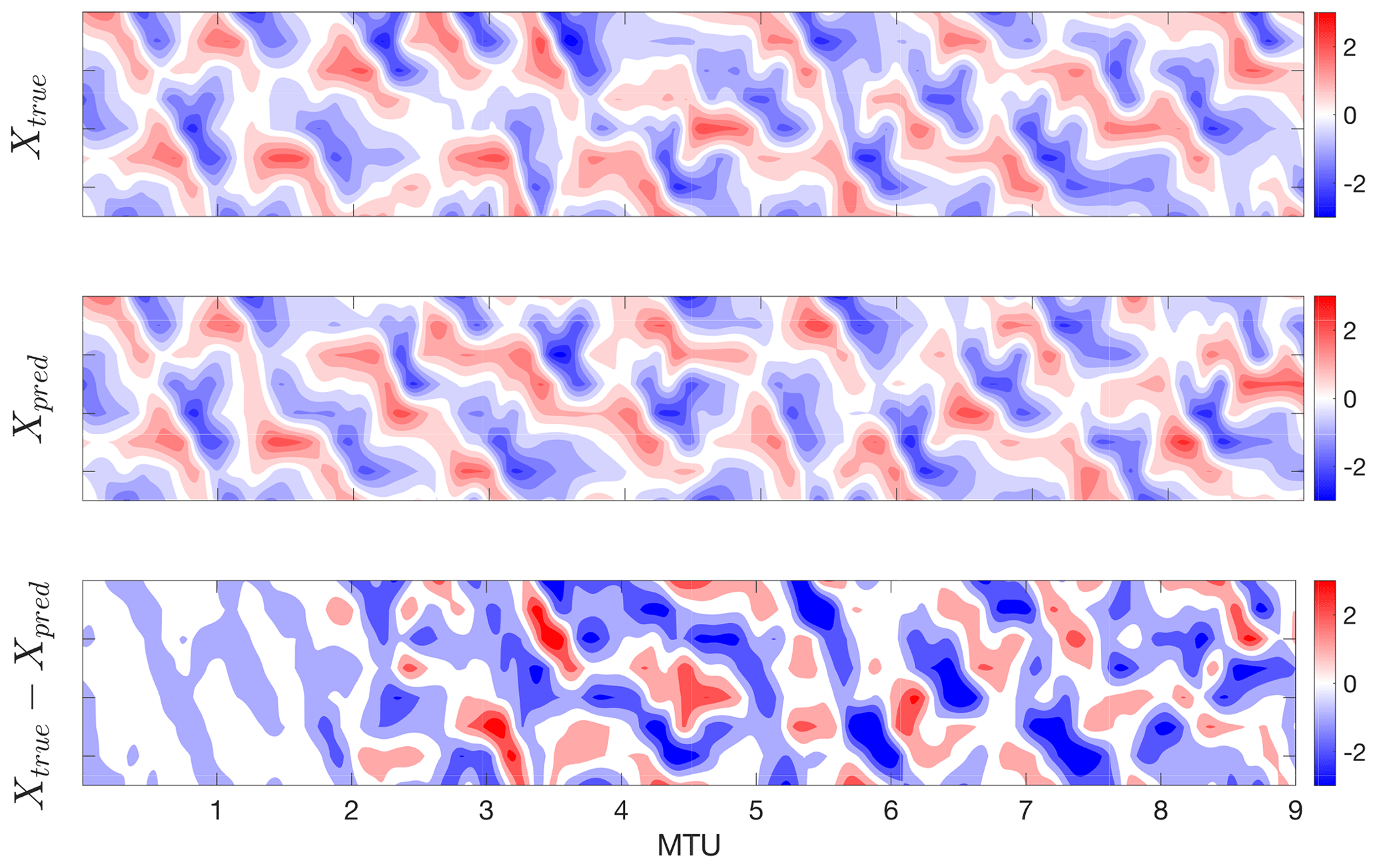
Figure 6 Performance of RC–ESN for short-term spatiotemporal predictions. We remind the readers that only the slow/large-scale variable X has been used during training/testing, and the fast/small-scale variables Y and Z have not been used at any point during training or testing. RC–ESN has substantial forecasting skills, providing accurate predictions up to ≈2 MTU, which is around 400Δt or 9 Lyapunov timescales. N=500 000, algorithm T₂, D=5000, and ρ=0.1 are used.

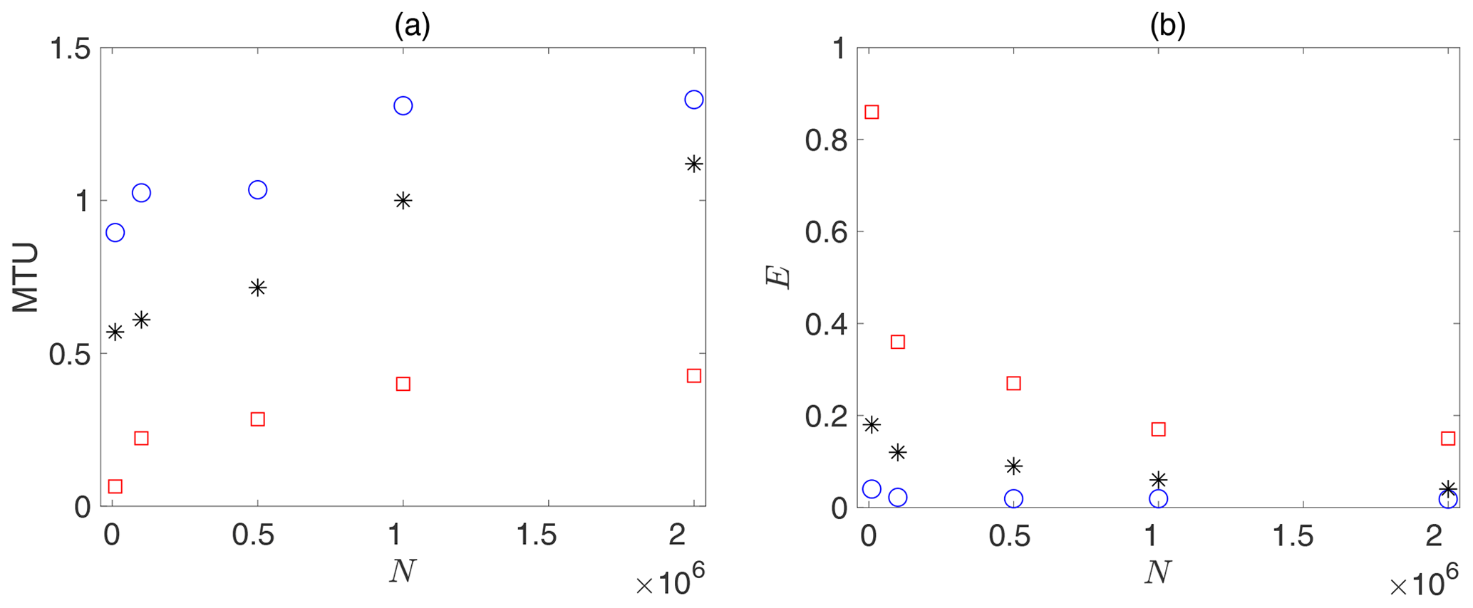
Figure 7 Comparison of the short-term predictions quality for RC–ESN (blue circles), RNN–LSTM (black stars), and ANN (red squares) as the size of the training set N is changed from N=10⁴ to $N=\mathrm{2}\times {\mathrm{10}}^{\mathrm{6}}$. Panel (a) shows the prediction horizon (when e(t) reaches 0.3), and panel (b) shows the average error E (see Eq. 9). The hyperparameters in each method are optimized for each N.

Overall, compared to both RNN–LSTM and ANN, the prediction horizon and accuracy of RC–ESN have a weaker dependence on the size of the training set, which is a significant advantage for RC–ESN when the dataset available for training is short, which is common in many practical problems.

3.3 Short-term predictions: scaling of RC–ESN performance with reservoir size D

Given the superior performance of RC–ESN for short-term predictions, here we focus on one concern with this method, namely the need for large reservoirs, which can be computationally demanding. This issue has been suggested as a potential disadvantage of ESNs versus LSTMs for training RNNs (Jaeger, 2007). Aside from the observation here that RC–ESN significantly outperforms RNN–LSTM for short-term predictions, the problem of reservoir size can be tackled in at least two ways. First, Pathak et al. (2018a) have proposed, and shown the effectiveness of, using a set of parallelized reservoirs, which allow one to easily deal with high-dimensional chaotic toy models.

Second, Fig. 8 shows that E rapidly declines by a factor of around 3 as D is increased from 500 to 5000, decreases slightly as D is further doubled to 10 000, and then barely changes as D is doubled again to 20 000. Training the RC–ESN with D=20 000 versus D=5000 comes with a higher computational cost (16 GB memory and ≈6 CPU hours for D=5000 and 64 GB memory and ≈18 CPU hours for D=20 000), while little improvement in accuracy is gained. Thus, concepts from inexact computing can be used to choose D so that precision is traded for large savings in computational resources, which can then be reinvested into more simulations, higher resolutions for critical processes, etc. (Palem, 2014; Palmer, 2014; Düben and Palmer, 2014; Leyffer et al., 2016; Thornes et al., 2017).

Figure 8 Scaling of average prediction error between 0 and 0.5 MTU (E; Eq. 9) with reservoir size D for RC–ESN. N=500 000 is used.

3.4 Long-term statistics: comparison of RC–ESN, ANN, and RNN–LSTM performance

All the data-driven predictions discussed earlier eventually diverge from the true trajectory (as would even predictions using the numerical solver). Still, it is interesting to examine whether the freely predicted spatiotemporal data have the same long-term statistical properties as the actual dynamical system (i.e., Eqs. 1–3). Reproducing the actual dynamical system's long-term statistics (sometimes referred to as the system's climate) using a data-driven method can be significantly useful. In some problems, a surrogate model does not need to predict the evolution of a specific trajectory but only the long-term statistics of a system. Furthermore, synthetic long datasets produced using an inexpensive data-driven method (trained on a shorter real dataset) can be used to examine the system's probability density functions (pdf's), including its tails, which are important for studying the statistics of rare/extreme events.

By examining return maps, Pathak et al. (2017) have already shown that RC–ESNs can reproduce the long-term statistics of the Lorenz 63 and Kuramoto–Sivashinsky equations. Jaeger and Haas (2004) and Pathak et al. (2017) have also shown that RC–ESNs can be used to accurately estimate a chaotic system's Lyapunov spectrum. Here, we focus on comparing the performance of RC–ESN, ANN, and RNN–LSTM in reproducing the system's long-term statistics by doing the following:

• examining the estimated pdf's and in particular their tails

• investigating whether the quality of the estimated pdf's degrades with time, which can negate the usefulness of long synthetic datasets.

Figure 9 compares the estimated pdf's obtained using the three ML methods. The data predicted using RC–ESN and RNN–LSTM are found to have pdf's closely matching the true pdf, even at the tails. Deviations at the tails of the pdf predicted by these methods from the true pdf are comparable to the deviations of the pdf's obtained from true data using the same number of samples. The ANN-predicted data have reasonable pdf's at ±2 standard deviation (SD), but the tails have substantial deviations from those of the true pdf's. All predicted pdf's are robust and do not differ much (except near the end of the tails) among the quartiles.

The results show that RC–ESN and RNN–LSTM can accurately reproduce the system's long-term statistics and can robustly produce long synthetic datasets with pdf's that are close to the pdf of the true data – even near the tails. The ability of ANN to accomplish these tasks is limited.

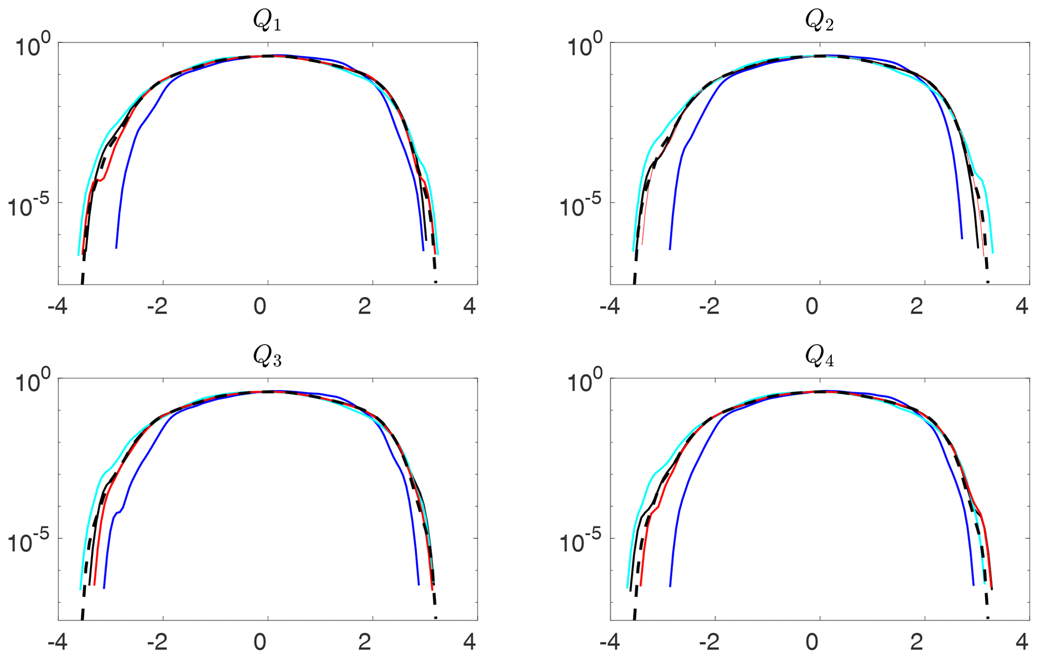
Figure 9 Estimated probability density functions (pdf's) of long datasets freely predicted by using RC–ESN (red), ANN (blue), and RNN–LSTM (cyan) compared to the true pdf (broken black). RC–ESN, ANN, and RNN–LSTM are first trained with N=500 000 and then predict, from an initial condition, for 4×10⁶Δt. Panels Q₁−Q₄ correspond to the equally divided quartiles of 10⁶ predicted samples. The pdf's are approximated using kernel density estimation (Epanechnikov, 1969). The green lines show the estimated pdf's from different sets of 10⁶ samples that are obtained from the numerical solution of Eqs. (1)–(3). Small differences between the green lines show the uncertainties in estimating the tails from 10⁶ samples. The broken black lines show the true pdf estimated from 10⁷ samples from the numerical solution. Note that the presented pdf's are for standardized data.

4 Discussion

By examining the true and predicted trajectories (Figs. 5–6) and the prediction errors and horizons (Fig. 7), we have shown that RC–ESN substantially outperforms ANN and RNN–LSTM in predicting the short-term evolution of a multiscale Lorenz 96 chaotic system (Eqs. 1–3). Additionally, RC–ESN and RNN–LSTM both work well in reproducing the long-term statistics of this system (Fig. 9). We emphasize that, following the problem formulation of Dueben and Bauer (2018), and unlike most other studies, only part of the multiscale state vector (the slow/large-scale variable X) has been available for training the data-driven model and has been of interest for testing. This problem design is more relevant to many practical problems but is more challenging as it requires the data-driven model to not only predict the evolution of X based on its past observations but also to account for the effects of the intermediate and fast/small-scale variables Y and Z on X.

We have also found that the prediction horizon of RC–ESN, and even more so its prediction accuracy, to weakly depend on the size of the training set (Fig. 7). This is an important property as in many practical problems the data available for training are limited. Furthermore, the prediction error of RC–ESN is shown to have an asymptotic behavior for large reservoir sizes, which suggests that reasonable accuracy can be achieved with moderate reservoir sizes. Note that the skillful predictions with RC–ESN in Figs. 5–6 have been obtained with a moderate-sized training set (N=500 000) and reservoir (D=5000). Figures 7 and 8 suggest that slightly better results could have been obtained using larger N and D, although such improvements come at a higher computational cost during training.

The order we have found for the performance of the three machine-learning methods (RC–ESN > RNN–LSTM > ANN) is different from the order of complexity of these methods in terms of the number of trainable parameters (RC–ESN < ANN < RNN–LSTM). But the order of performance is aligned with the order in terms of the learnable function space, namely ANN < RC–ESN and RNN–LSTM. The latter methods are both RNNs and thus Turing complete, while ANN is a stateless feed-forward network and thus not Turing complete (Siegelmann and Sontag, 1992). The Turing completeness of RNNs, in theory, enables RNNs to compute any function or implement any algorithm. Furthermore, state augmentation of ANN is not possible because it has no state. Whether the superior predictive performance of RC–ESN (especially over RNN–LSTM) is due to its explicit state representation, which is updated at every time step during both training and testing, or its lower likelihood of overfitting due to the order of magnitude having a smaller number of trainable parameters remains to be seen. Also, whether we have fully harnessed the power of RNN–LSTMs (see below) is unclear at this point, particularly because a complete theoretical understanding of how/why these methods work (or do not work) is currently lacking. That said, there has been some progress in understanding the RC–ESNs, in particular by modeling the network itself as a dynamical system (Yildiz et al., 2012; Gauthier, 2018). Such efforts, for example those aimed at understanding the echo states that are learned in the RC–ESN's reservoir, might benefit from recent advances in dynamical systems theory, e.g., for analyzing nonlinear spatiotemporal data (Mezić, 2005; Tu et al., 2014; Williams et al., 2015; Arbabi and Mezic, 2017; Giannakis et al., 2017; Khodkar and Hassanzadeh, 2018).

An important next step in our work is to determine how generalizable our findings are. This investigation is important for the following two reasons. First, here we have only studied one system, which is a specially designed version of the Lorenz 96 system. The performance of these methods should be examined in a hierarchy of chaotic dynamical systems and high-dimensional turbulent flows. That said, our findings are overall consistent with the recently reported performance of these methods applied to chaotic toy models. It has been demonstrated that RC–ESN can predict, for several Lyapunov timescales, the spatiotemporal evolution and can reproduce the climate of the Lorenz 63 and Kuramoto–Sivashinsky chaotic systems (Pathak et al., 2017, 2018a; Lu et al., 2017). Here, we have shown that RC–ESN performs similarly well even when only the slow/large-scale component of the multiscale state vector is known. Our results with ANN are consistent with those of Dueben and Bauer (2018), who showed examples of trajectories predicted accurately up to 1 MTU with a large training set ($N=\mathrm{2}\times {\mathrm{10}}^{\mathrm{6}}$) and using ANN for the same Lorenz 96 system (see their Fig. 1). While RNN–LSTM is considered to be state of the art for sequential data modeling, and has worked well for a number of applications involving time series to the best of our knowledge, simple RNN–LSTMs, such as the one used here, have not been very successful when applied to chaotic dynamical systems. Vlachas et al. (2018) found some prediction skills, using RNN–LSTM applied to the original Lorenz 96 system, which does not have the multiscale coupling (see their Fig. 5).

Second, we have only used a simple RNN–LSTM. There are other variants of this architecture and more advanced deep-learning RNNs that might potentially yield better results. For our simple RNN–LSTM, we have extensively explored the optimization of hyperparameters and tried various formulations of the problem, e.g., predicting ΔX(t) with or without updating the state of the LSTM. We have found that such variants do not lead to better results, which is consistent with the findings of Vlachas et al. (2018). Our preliminary explorations with more advanced variants of RNN–LSTM, e.g., seq2seq and encoder-decoder LSTM (Sutskever et al., 2014), have not resulted in any improvement either. However, just as the skillful predictions of RC–ESN and ANN hinge on one key step (nonlinear transformation for the former and predicting ΔX for the latter), it is possible that changing/adding one step leads to major improvements in RNN–LSTM. It is worth mentioning that similar nonlinear transformation of the state in LSTMs is not straightforward due to their more complex architecture; see Appendix D. We have shared our codes publicly to help others explore such changes to our RNN–LSTM. Furthermore, there are other, more sophisticated RNNs that we have not yet explored. For example, Yu et al. (2017) have introduced a tensor-train RNN that outperformed a simple RNN–LSTM in predicting the temporal evolution of the Lorenz 63 chaotic system. Mohan et al. (2019) showed that a compressed convolutional LSTM performs well in capturing the long-term statistics of a turbulent flow. The performance of more advanced deep-learning RNNs should be examined and compared, side by side, with the performance of RC–ESNs and ANNs in future studies. The multiscale Lorenz 96 system provides a suitable starting point for such comparisons.

The results of our work show the promise of ML methods, such as RC–ESNs (and to some extent RNN–LSTM), for data-driven modeling of chaotic dynamical systems, which have broad applications in geosciences, e.g., in weather and climate modeling. Practical and fundamental issues such as interpretability; scalability to higher-dimensional systems (Pathak et al., 2018a); presence of measurement noise in the training data and initial conditions (Rudy et al., 2018); nonstationarity of the time series; and dealing with data that have two or three spatial dimensions (e.g., through integration with convolutional neural networks, namely CNN–LSTM, (Xingjian et al., 2015) and CNN–ESN (Ma et al., 2017) should be studied in future work).

Here we have focused on a fully data-driven approach, as opposed to the conventional approach of the direct numerical solutions (Fig. 2). In practice, for example, for large-scale multiphysics, multiscale dynamical systems such as weather and climate models, it is likely that a hybrid framework yields the best performance. In such a framework, depending on the application and the spatiotemporal scales of the physical processes involved (Thornes et al., 2017; Chantry et al., 2019), some of the equations could be solved numerically with double precision, some could be solved numerically with lower precisions, and some could be approximated with a surrogate model learned via a data-driven approach, such as the ones studied in this paper.

Appendix A: More details on RC–ESN

Here we show a comparison of RC–ESN forecasting skills with nonlinear transformation algorithms T₁ (Pathak et al., 2018a), T₂, and T₃ and without any transformation between r and $\stackrel{\mathrm{̃}}{\mathbf{r}}$. The three algorithms are (for $i=\mathrm{1},\mathrm{2},\mathrm{3}\mathrm{\dots }N$ and $j=\mathrm{1},\mathrm{2},\mathrm{3}\mathrm{\dots }D$) as follows:

Algorithm T₁

$$\begin{array}{llll}{\displaystyle }& {\displaystyle }{\stackrel{\mathrm{̃}}{\mathbf{r}}}_{i,j}={\mathbf{r}}_{i,j}\times {\mathbf{r}}_{i,j}& {\displaystyle }& {\displaystyle }\text{ if }j\text{ is odd; }\\ {\displaystyle }& {\displaystyle }{\stackrel{\mathrm{̃}}{\mathbf{r}}}_{i,j}={\mathbf{r}}_{i,j}& {\displaystyle }& {\displaystyle }\text{ if }j\text{ is even, }\end{array}$$

Algorithm T₂

$$\begin{array}{llll}{\displaystyle }& {\displaystyle }{\stackrel{\mathrm{̃}}{\mathbf{r}}}_{i,j}={\mathbf{r}}_{i,j-\mathrm{1}}\times {\mathbf{r}}_{i,j-\mathrm{2}}& {\displaystyle }& {\displaystyle }\text{ if }j>\mathrm{1}\text{ is odd; }\\ {\displaystyle }& {\displaystyle }{\stackrel{\mathrm{̃}}{\mathbf{r}}}_{i,j}={\mathbf{r}}_{i,j}& {\displaystyle }& {\displaystyle }\text{ if }j\text{ is 1 or even.}\end{array}$$

Algorithm T₃

$$\begin{array}{llll}{\displaystyle }& {\displaystyle }{\stackrel{\mathrm{̃}}{\mathbf{r}}}_{i,j}={\mathbf{r}}_{i,j-\mathrm{1}}\times {\mathbf{r}}_{i,j+\mathrm{1}}& {\displaystyle }& {\displaystyle }\text{ if }j>\mathrm{1}\text{ is odd; }\\ {\displaystyle }& {\displaystyle }{\stackrel{\mathrm{̃}}{\mathbf{r}}}_{i,j}={\mathbf{r}}_{i,j}& {\displaystyle }& {\displaystyle }\text{ if }j\text{ is 1 or even. }\end{array}$$

Figure A1a shows an example of short-term predictions from an initial condition using T₁, T₂, T₃, and no transformation; everything else was kept the same. It is clear that the nonlinear transformation is essential for skillful predictions, as the predictions obtained without transformation diverge from the truth before 0.25 MTU. The three nonlinear transformation algorithms yield similar results, with accurate predictions for more than 2 MTU. Figure A1b, which shows the relative prediction error averaged over 100 initial conditions, further confirms this point.

Why the nonlinear transformation is needed, and the best/optimal choice for the transformation (if it exists), should be studied in future work. We highlight that the nonlinear transformation resembles basis function expansion, which is commonly used to capture nonlinearity in linear regression models (Bishop, 2006).

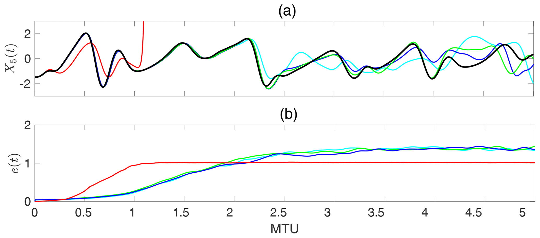
Figure A1 Comparison of RC–ESN forecasting skills with nonlinear transformation algorithms T₁, T₂, and T₃ (cyan, green, and blue lines, respectively) and without any transformation (red line). Black line shows the truth. (a) Predictions from one initial condition and (b) relative L₂-norm error averaged over 100 initial condition e(t) (Eq. 8). Time is in MTU, where $\mathrm{1}\mathrm{MTU}=\mathrm{200}\mathrm{\Delta }t\approx \mathrm{4.5}/{\mathit{\lambda }}_{max}$.

Appendix B: Dependence of RC–ESN's prediction horizon on ρ

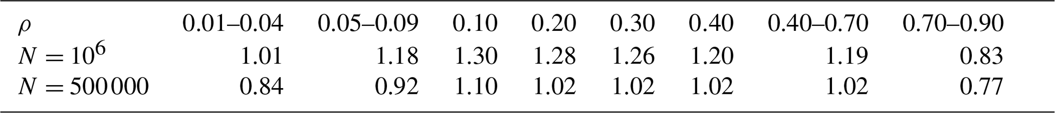
We have conducted an extensive experimental analysis of the dependence of RC–ESN's prediction horizon on the value of ρ and found ρ=0.1 to produce the best prediction horizon for any sample size, N, and reservoir size, D, for this system. Table B1 shows part of the results obtained from the experiments with N=500 000, N=10⁶, and with D=5000 over 100 initial conditions. While ρ=0.1 yields the best results, we see that the prediction horizon is barely sensitive to the choice of ρ within a wide range and similar overall prediction horizons are obtained for $\mathrm{0.05}\le \mathit{\rho }\le \mathrm{0.7}$.

Table B1 Prediction horizon (MTU) over 100 initial conditions for an RC–ESN with samples sizes of N=10⁶, N=500 000, and D=5000 for different ranges of ρ.

Appendix C: More details on ANN

The ANN used in this study (and the one that yields the best performance) is similar to that of Dueben and Bauer (2018). The ANN has four hidden layers, each of which has 100 neurons with a tanh activation function. The input to the ANN has 8 neurons which takes (X(t))^test as the input and outputs (ΔX(t))^test which is also a 8-neuron layer. The obtained (ΔX(t))^test output during the test is then used in an Adams–Bashforth integration scheme to obtain (X(t+Δt))^test. We found that a simpler Euler scheme yields similar results. However, we found that training/testing on pairs of X(t) and X(t+Δt), which was used for RC–ESN, leads to no prediction skill with ANN, and that following the procedure used in Dueben and Bauer (2018) is essential for skillful predictions. We speculate that this might be due to the stateless nature of the ANN. By relating X(t) to the change in X(t) at the next time step, rather than the raw value X(t+Δt), this ANN training architecture implicitly contains a reference to the previous time step. While the ANN itself is stateless, this particular training approach essentially encodes a first-order temporal dependence between successive states.

Note that our approach here is the same as the global ANN of Dueben and Bauer (2018). We also tried their local ANN approach but, consistent with their findings for the Lorenz system, found better performance with the global approach (results not reported for brevity).

The ANN is trained with a stochastic gradient descent algorithm with a learning rate of 0.001, with a batch size of 100, and mean absolute error as the loss function (mean squared error also gives similar performance).

Appendix D: More details on RNN–LSTM

The governing equations for RNN–LSTM are as follows:

$$\begin{array}{}\text{(D1)}& {\displaystyle }& {\displaystyle }{g}^f\left(t\right)={\mathit{\sigma }}_f\left({\mathbf{W}}_{\mathbf{f}}\left[h(t-\mathrm{1}),I\left(t\right)\right]+b_f\right),\text{(D2)}& {\displaystyle }& {\displaystyle }{g}^i\left(t\right)={\mathit{\sigma }}_f\left({\mathbf{W}}_{\mathbf{i}}\left[h(t-\mathrm{1}),I\left(t\right)\right]+b_i\right),\text{(D3)}& {\displaystyle }& {\displaystyle }\stackrel{\mathrm{̃}}{C}\left(t\right)=\tanh \left({\mathbf{W}}_{\mathbf{c}}\left[h(t-\mathrm{1}),I\left(t\right)\right]+b_h\right),\text{(D4)}& {\displaystyle }& {\displaystyle }C\left(t\right)=g^f\left(t\right)C(t-\mathrm{1})+g^i\left(t\right)\stackrel{\mathrm{̃}}{C}\left(t\right),\text{(D5)}& {\displaystyle }& {\displaystyle }{g}^o\left(t\right)={\mathit{\sigma }}_h\left({\mathbf{W}}_{\mathbf{h}}\left[h(t-\mathrm{1}),I\left(t\right)\right]+b_h\right),\text{(D6)}& {\displaystyle }& {\displaystyle }h\left(t\right)=g^o\left(t\right)\tanh \left(C\left(t\right)\right),\text{(D7)}& {\displaystyle }& {\displaystyle }\mathrm{\Phi }\left(t\right)={\mathbf{W}}_{\mathbf{oh}}h\left(t\right),\text{(D8)}& {\displaystyle }& {\displaystyle }X(t+\mathrm{\Delta }t)\approx \mathrm{\Phi }\left(t\right).\end{array}$$

σ_f is the softmax activation function and g^f(t), gⁱ(t), and g^o(t) $\in {\mathrm{\Re }}^{d_h\times \left(d_h+d_i\right)}$ are the forget gate, input gate, and output gate, respectively. d_h is the dimension of the hidden layers (chosen as 50 in our study), and d_i is the dimension of the input (8×q). b_f, b_i, and b_h are the biases in the forget gate, input gate, and the hidden layers. $I\left(t\right)\in {\mathrm{\Re }}^{d_i}$ is the input, which is a column of a time-delay-embedded matrix of X(t). This matrix has the dimension of $(\mathrm{8}\times q)\times N$. $h\left(t\right)\in {\mathrm{\Re }}^{d_h}$ is the hidden state and $C\left(t\right)\in {\mathrm{\Re }}^{d_h}$ is the cell state (the states track the temporal evolution). The weights W_o, W_i, W_f, W_c, and W_oh are learned through the BPTT algorithm (Goodfellow et al., 2016) using an Adam optimizer (Kingma and Ba, 2014). Φ(t) is the output from the RNN–LSTM.

The LSTM used in this study is a stateless LSTM, in which the two hidden states (C and h) are refreshed at the beginning of each batch during training (this is not the same as the stateless ANN, where there is no hidden state at all). Here, the training sequences in each batch are shuffled randomly, leading to an unbiased gradient estimator in the stochastic gradient descent algorithm (Meng et al., 2019).