Simulating model uncertainty of subgrid-scale processes by sampling model errors at convective scales

Ideally, perturbation schemes in ensemble forecasts should be based on the statistical properties of the model errors. Often, however, the statistical properties of these model errors are unknown. In practice, the perturbations are pragmatically modelled and tuned to maximize the skill of the ensemble forecast.

In this paper a general methodology is developed to diagnose the model error, linked to a specific physical process, based on a comparison between a target and a reference model. Here, the reference model is a configuration of the ALADIN (Aire Limitée Adaptation Dynamique Développement International) model with a parameterization of deep convection. This configuration is also run with the deep-convection parameterization scheme switched off, degrading the forecast skill. The model error is then defined as the difference of the energy and mass fluxes between the reference model with scale-aware deep-convection parameterization and the target model without deep-convection parameterization.

In the second part of the paper, the diagnosed model-error characteristics are used to stochastically perturb the fluxes of the target model by sampling the model errors from a training period in such a way that the distribution and the vertical and multivariate correlation within a grid column are preserved. By perturbing the fluxes it is guaranteed that the total mass, heat and momentum are conserved.

The tests, performed over the period 11–20 April 2009, show that the ensemble system with the stochastic flux perturbations combined with the initial condition perturbations not only outperforms the target ensemble, where deep convection is not parameterized, but for many variables it even performs better than the reference ensemble (with scale-aware deep-convection scheme). The introduction of the stochastic flux perturbations reduces the small-scale erroneous spread while increasing the overall spread, leading to a more skillful ensemble. The impact is largest in the upper troposphere with substantial improvements compared to other state-of-the-art stochastic perturbation schemes. At lower levels the improvements are smaller or neutral, except for temperature where the forecast skill is degraded.

1 Introduction

Numerical weather prediction (NWP) is an initial value problem with models based on equations that describe the evolution of the atmospheric state and its interaction with other Earth system components. The solution of these equations is highly sensitive to the initial conditions (e.g. Thompson, 1957; Lorenz, 1969; Vannitsem and Nicolis, 1997; Buizza and Leutbecher, 2015). As a result, the errors made in the initial conditions will lead to forecast error growth and eventually to a loss of predictability.

Quantification of the forecast uncertainty due to the uncertainty in the initial conditions is often done through ensemble-based Monte Carlo simulations. It has been shown that such Monte Carlo simulations, representing initial uncertainties consistent with the true distribution of initial condition errors, are typically under-dispersive and therefore lack reliability (e.g. Wilks, 2005; Palmer et al., 2005). This has motivated the research for methodologies to represent the uncertainties related to the model description in addition to the uncertainty in initial conditions.

The many needed simplifications and approximations made in NWP models also contribute to the forecast error evolution (Lorenz, 1982; Dalcher and Kalnay, 1987; Orrel, 2002; Vannitsem and Toth, 2002; Nicolis, 2003, 2004; Nicolis et al., 2009). These model imperfections, arising from incomplete knowledge of physical processes, finite resolution, uncertain parameters in parameterizations and discretization, will also lead to a reduction in predictability even if the initial state would correspond exactly to the true state of the atmosphere. This category of errors, including filtering operations mapping the true atmospheric state onto the state space of the model, is defined as the model error (Leutbecher et al., 2017). Recently, much effort has been put into the development of schemes that simulate the random component of the errors of the model tendencies.

A first operational development of such a representation of model uncertainty was done by Buizza et al. (1999). Their scheme, generally referred to as the stochastically perturbed parameterization tendency (SPPT) scheme, makes the assumption that the dominant part of the parameterized physics tendency error is proportional to the net physics tendency. Major revisions of the scheme were done by Palmer et al. (2009) and Shutts et al. (2011) both changing aspects of the probability distribution sampled by the SPPT scheme.

Another type of model uncertainty is addressed by Shutts (2005) and Berner et al. (2009). In their work, the focus lies on the model uncertainty associated with scale interactions that are present in the real atmosphere but absent in the model due to its finite resolution. To represent this uncertainty, they developed the stochastic kinetic energy backscatter (SKEB) scheme, which introduces a stochastic streamfunction forcing determined by a local estimate of kinetic energy sources at the subgrid scale together with an evolving three-dimensional pattern.

A different approach to account for model uncertainty is to perturb a set of key parameters within the parameterization schemes themselves. This technique was first applied in Bowler et al. (2008) and further adapted for use in a convection-permitting ensemble by Baker et al. (2014). The concept of stochastically perturbing parameters was further generalized in the stochastically perturbed parameterization (SPP) scheme (Ollinaho et al., 2013, 2017). SPP extends the concept of perturbing parameters to locally perturbing both parameters and variables inside the parameterizations.

Keeping in mind the purpose of stochastic perturbations, which is to represent forecast uncertainties originating from model errors, the perturbations ideally have the same statistics as the error source. Since the model error sources are diverse and their statistical characteristics only partially known (Boisserie et al., 2014), the methods described above resort to pragmatic solutions: the amplitude of the perturbations or their spatial patterns are usually chosen such that a satisfactory reduction of ensemble under-dispersion is obtained (Berner et al., 2017).

Recent methods to assess sources of model uncertainty and their statistical properties are based on a comparison between perfect and target forecasts (Nicolis, 2003, 2004; Nicolis et al., 2009). This approach has been adopted in Seiffert et al. (2006) by comparing high- and low-resolution global circulation model (GCM) runs, or in Shutts and Pallarès (2014) by comparing the temperature tendencies associated with convection parameterizations in high and low resolution forecasts of the European Centre for Medium-Range Weather Forecasts (ECMWF) Integrated Forecast System (IFS).

The aim of the present paper is to use this method to characterize the model error related to a specific physical process by comparing two forecasts which differ only in the representation of the physical process under investigation. First a general description of the methodology is given, after which it is applied to deep convection. This is done by running the ALADIN (Aire Limitée Adaptation Dynamique Développement International) limited area model (LAM) (Termonia et al., 2018) in a configuration where deep convection is not parameterized and comparing it to a reference configuration with a scale-aware deep-convection parameterization scheme. The simulations are performed over the tropics during a period of enhanced convective activity on a grid with a horizontal grid spacing of 4 km. This resolution lies on the verge of what is considered the convection-permitting scale, where it has been demonstrated (Deng and Stauffer, 2006; Lean et al., 2008; Roberts and Lean, 2008) that non-parameterized convection often shows unrealistically strong updrafts and density currents as well as overestimated precipitation rates.

The model error is expressed in the form of a flux difference and its characteristics are obtained from a well-chosen training period. After discussing the statistical properties of the model error, its usefulness for probabilistic forecasting is investigated by developing a prototype stochastic flux perturbation scheme. The scheme introduces flux perturbations by sampling the model error from the training period. The impact of perturbing the fluxes, using the properties of the model error, on a short-range (48 h) LAM forecast is then studied, revealing a positive impact on the forecast quality.

The structure of this paper is as follows. The methodology for quantifying the model error and its statistical properties are presented in Sect. 2. In Sect. 3 the design of the perturbation scheme is described and the results of its application are discussed. Finally, the main results are summarized and conclusions are drawn in Sect. 4.

2 Quantification of the model error

2.1 Methodology for a high-order NWP model

In the theoretical work on generic dynamical low-order models (Nicolis, 2003, 2004; Nicolis et al., 2009) the behaviour of the model error is investigated by comparing the evolution laws of an approximating model with the exact evolution laws. For these low-order problems, both the model and exact evolution laws can be written in an analytical form. This is formally done as follows. First, one writes

$$\begin{array}{}\text{(1)}& {\displaystyle \frac{\mathrm{d}\mathbf{X}}{\mathrm{d}t}}=\mathbf{f}\left(\mathbf{X}\right),\text{(2)}& {\displaystyle \frac{\mathrm{d}\mathbf{Y}}{\mathrm{d}t}}=\mathbf{g}\left(\mathbf{Y}\right),\end{array}$$

where X represents the exact solution of the perfect model f and Y the solution of the model g. Then, starting from identical initial conditions X(t₀)=Y(t₀) one can write for a sufficiently small time interval δt

$$\begin{array}{}\text{(3)}& {\displaystyle }\mathbf{X}(t_{\mathrm{0}}+\mathit{\delta }t)=\mathbf{X}\left(t_{\mathrm{0}}\right)+\mathbf{f}\left(\mathbf{X}\right(t_{\mathrm{0}}\left)\right)\mathit{\delta }t,\text{(4)}& {\displaystyle }\mathbf{Y}(t_{\mathrm{0}}+\mathit{\delta }t)=\mathbf{X}\left(t_{\mathrm{0}}\right)+\mathbf{g}\left(\mathbf{X}\right(t_{\mathrm{0}}\left)\right)\mathit{\delta }t.\end{array}$$

The model error can be written as $\mathbf{U}\left(t\right)\equiv \mathbf{Y}\left(t\right)-\mathbf{X}\left(t\right)$ by extracting Eq. (3) from Eq. (4):

$$\begin{array}{}\text{(5)}& \mathbf{U}(t+\mathit{\delta }t)=\left(\mathbf{g}\left(\mathbf{X}\right(t_{\mathrm{0}}\left)\right)-\mathbf{f}\left(\mathbf{X}\right(t_{\mathrm{0}}\left)\right)\right)\mathit{\delta }t.\end{array}$$

The model error source, determining the short time behaviour of U, is then characterized by estimating

$$\begin{array}{}\text{(6)}& \mathit{ϵ}=\mathbf{g}\left(\mathbf{X}\right)-\mathbf{f}\left(\mathbf{X}\right).\end{array}$$

Of course, when dealing with the comparison of the evolution operator of an NWP model and reality, the model error cannot be formally expressed as the underlying dynamics of the reality are not fully known. Nevertheless the same formal approach can be applied to quantify the model errors that are caused by poor choices in the model formulation compared to well-performing ones of a reference version. In practice this is done by

1. running a validated reference configuration of a full NWP model,

2. switching off one of the parameterizations (or replacing it with a poor choice) to create a target of study,

3. verifying with standard NWP scores that the target configuration performs less well than the reference configuration, and

4. computing the model error.

In this case we consider the reference as a perfect model corresponding to the model f in Eq. (1), while the target model now becomes the one in Eq. (2). We then define the model error as in Eq. (6).

Here we apply this method to quantify the model error related to a specific parameterization of a subgrid process. The formulations of both models differ only in the representation of the physical process under consideration. Other parameters, such as the time step and vertical and horizontal resolution, are kept identically. Finally, both models start from the same initial model state, and the error is evaluated over a single time step. The model error obtained in this way can then be seen as a source of model uncertainty of the subgrid processes. It will then be shown how its properties can serve as a guide when developing stochastic perturbation schemes.

We will apply this method to simulations with the ALADIN NWP model, using the ALARO (ALADIN-AROME) canonical configuration (Termonia et al., 2018), henceforth called the ALARO model. The model can be run both in a hydrostatic and a non-hydrostatic configuration and uses a spectral dynamical core with a two-time-level semi-Lagrangian semi-implicit scheme. The vertical discretization uses a mass-based hybrid pressure terrain-following coordinate. An overview of the parameterization schemes used and a description of the scale-aware deep-convection parameterization can be found in Appendix A.

The proposed methodology is generic and can be applied to all physical processes that can be represented by multiple schemes within the same model (e.g. radiation, turbulence, condensation, microphysics). However, in this paper, it is applied to the representation of deep convection in a model with a horizontal grid spacing of 4 km. The reference model uses a scale-aware deep convective parameterization, called 3MT (Gerard et al., 2009). This scheme has been developed specifically for the convection-permitting transition regime within the so-called grey zone of deep convection (Yano et al., 2018). These are horizontal resolutions where deep convection is not entirely resolved by the dynamics. As such the parameterization accounts for some subgrid transport that would be handled by the dynamics at fully convection-resolving resolutions. In operational applications with resolutions of about 4–5 km, the ALARO model is usually run with the hydrostatic set-up of the dynamical core.

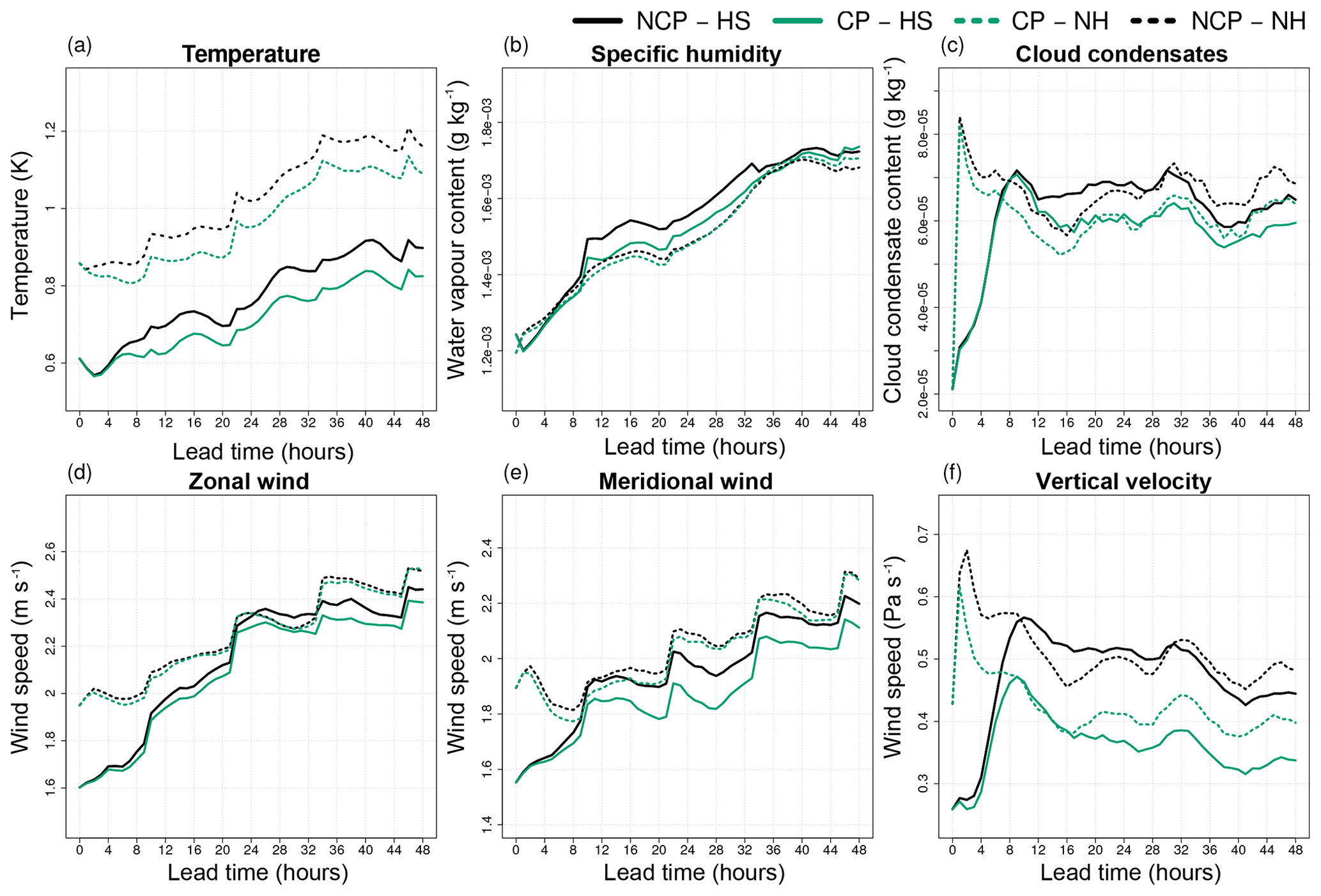
Figure 1 RMSE, defined in Appendix B, at 850 hPa of the ensemble simulation as described in Sect. 3.2 with the deep-convection scheme switched on (CP: green line) vs. the one with the parameterization switched off (NCP: black line). The full lines represent the simulations with the hydrostatic dynamics while the dotted lines represent the ones with the non-hydrostatic dynamics. The CP configuration performs best and is considered as the reference.

For the target set-up we switch off the 3MT scheme. Fig. 1 shows, for the experimental set-up that will be described in Sect. 3.2, that switching off the deep-convection scheme leads to a significant degradation of the model performance, both for the hydrostatic configuration and the non-hydrostatic configuration. So the computed model error can be seen as an error with respect to the operational reference. Moreover, it can be seen that the hydrostatic version performs better than the non-hydrostatic one, which does not come as a surprise since the entire ALARO model configuration including the deep-convection parameterization has been tuned with the hydrostatic option of the dynamical core. It is also useful to note that the error correction between the simulation with deep-convection parameterization and the one without is largest for the hydrostatic simulations, which confirms the above statement that the parameterization somehow compensates for non-hydrostatic subgrid effects. Verification scores for the 250 hPa (not shown) lead to the same conclusions. Therefore, in this paper, the hydrostatic version of the model will be used as the reference when computing the model error.

Within the ALARO model configuration the physics–dynamics coupling is organized in a flux-conservative way according to the proposal of Catry et al. (2007), where the contributions from the different physics parameterizations appear as fluxes in the thermodynamic energy equation. This allows the expression of the model errors of Eq. (6) between the simulation without deep convection and the one with deep-convection parameterization in terms of the fluxes instead of tendencies. Here we use the following definition:

$$\begin{array}{}\text{(7)}& {\displaystyle }{\mathit{ϵ}}_{\mathit{\psi }}^{\mathrm{trans}}={J^{\prime }}_{\mathit{\psi }}^{\mathrm{td}}-(J_{\mathit{\psi }}^{\mathrm{td}}+J_{\mathit{\psi }}^{\mathrm{c}})& {\displaystyle }\mathrm{with}\mathit{\psi }=q_{\mathrm{v}},q_{\mathrm{l}},q_{\mathrm{i}},h,u,v,\text{(8)}& {\displaystyle }{\mathit{ϵ}}_{\mathit{\phi }}^{\mathrm{cond}}={F^{\prime }}_{\mathit{\phi }}^{\mathrm{st}}-(F_{\mathit{\phi }}^{\mathrm{st}}+F_{\mathit{\phi }}^{\mathrm{c}})& {\displaystyle }\mathrm{with}\mathit{\phi }=\mathrm{vl},\mathrm{vi},\text{(9)}& {\displaystyle }{\mathit{ϵ}}_{\mathit{\varphi }}^{\mathrm{evap}}=F_{\mathit{\varphi }}^{\prime }-(F_{\mathit{\varphi }}^{\mathrm{st}}+F_{\mathit{\varphi }}^{\mathrm{c}})& {\displaystyle }\mathrm{with}\mathit{\varphi }=\mathrm{rv},\mathrm{sv},\end{array}$$

where $J_{\mathit{\psi }}^{\mathrm{td}}$ and $J_{\mathit{\psi }}^{\mathrm{c}}$ represent the turbulent diffusion and convective transport flux respectively of water vapour (q_v), cloud water (q_l), cloud ice (q_i), enthalpy (h), and zonal (u) and meridional (v) momentum. $F_{\mathit{\phi }}^{\mathrm{st}}$ and $F_{\mathit{\phi }}^{\mathrm{c}}$ represent the stratiform and convective condensation flux from water vapour to cloud water (vl) and from water vapour to cloud ice (vi). Stratiform and convective evaporation fluxes from rain to water vapour (rv) and snow to water vapour (sv) are denoted by $F_{\mathit{\varphi }}^{\mathrm{st}}$ and $F_{\mathit{\varphi }}^{\mathrm{c}}$, respectively. Non-primed fluxes are those obtained when running with deep-convection parameterization while primed fluxes represent those using no deep-convection parameterization. By defining the errors in this way one can see ϵ in Eqs. (7)–(9) as corrections to the turbulent fluxes to obtain the fluxes for the model with the deep-convection scheme switched on. Within the model they will appear under the vertical gradients of the Catry et al. (2007) formulation and will, by construction, conserve energy and mass.

In a numerical model, the time derivative in Eqs. (3) and (4) can be approximated by the evolution during a single model time step at t₀. For the model error to be correctly quantified, it is thus important that both reference and target model start from the same atmospheric state. For this reason one should use exactly the same model as the reference and the target model and only modify the source of the error, and nothing else. On the other hand, it is well known that NWP models suffer from spin-up periods during the first hours of the model runs when the model is still finding its physical balances. So taking initial model states immediately after the initial state may generate spurious tendencies which may lead to spurious errors in Eqs. (7)–(9). We solve this issue here by performing two parallel runs from identical initial conditions with the reference configuration. These identical simulations are given 12 h to spin up. After 12 h the deep-convection parameterization in one of the simulations is switched off and flux errors defined in Eqs. (7), (8) and (9) are diagnosed one time step later. In the next section it will be explained how this is implemented within the NWP model.

2.2 Construction of a model error database: implementation with an NWP model

The previous section explained how the model error due to the parameterization of deep convection can be quantified appropriately. This section describes how a database of model errors can be constructed.

In order to build a database with relevant weather cases (i.e. cases with active convection), the model simulations are performed over a tropical region including the Indian Ocean and Indonesia during a period of enhanced convective activity. The domain contains 1189×349 grid points and covers a region from 7^∘ S to 5.5^∘ N in the latitudinal direction and from 73.5 to 116^∘ E in the longitudinal direction (Fig. 2). The model has 46 vertical levels and is run with a time step of 300 s.

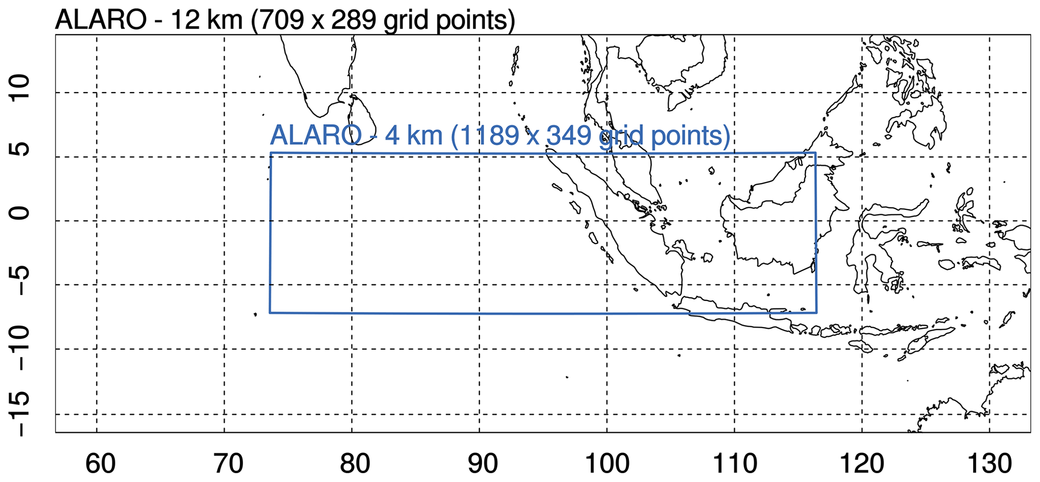
Figure 2 The ALARO 12 km grid spacing domain (outer black box) and the ALARO 4 km grid spacing domain (inner blue box).

The model runs are started every 3 h between 00:00 UTC 2 April 2009 and 21:00 UTC 10 April 2009. This period is described in Waliser et al. (2012) as a period of enhanced convective activity due to the presence of three active equatorial waves. Initial and boundary conditions are provided using a double-nesting technique where the ALARO model with a horizontal grid spacing of 12 km is driven by hourly ECMWF ERA 5 HRES analysis data (Copernicus Climate Change Service, 2017) and generates hourly initial conditions (ICs) and lateral boundary conditions (LBCs) for the 4 km simulations. The nesting from 12 to 4 km is shown in Fig. 2. Organizing the simulations this way leads to a total of 72 (9 d ×8 runs per day) evaluations of the model error at 8 different times in the day.

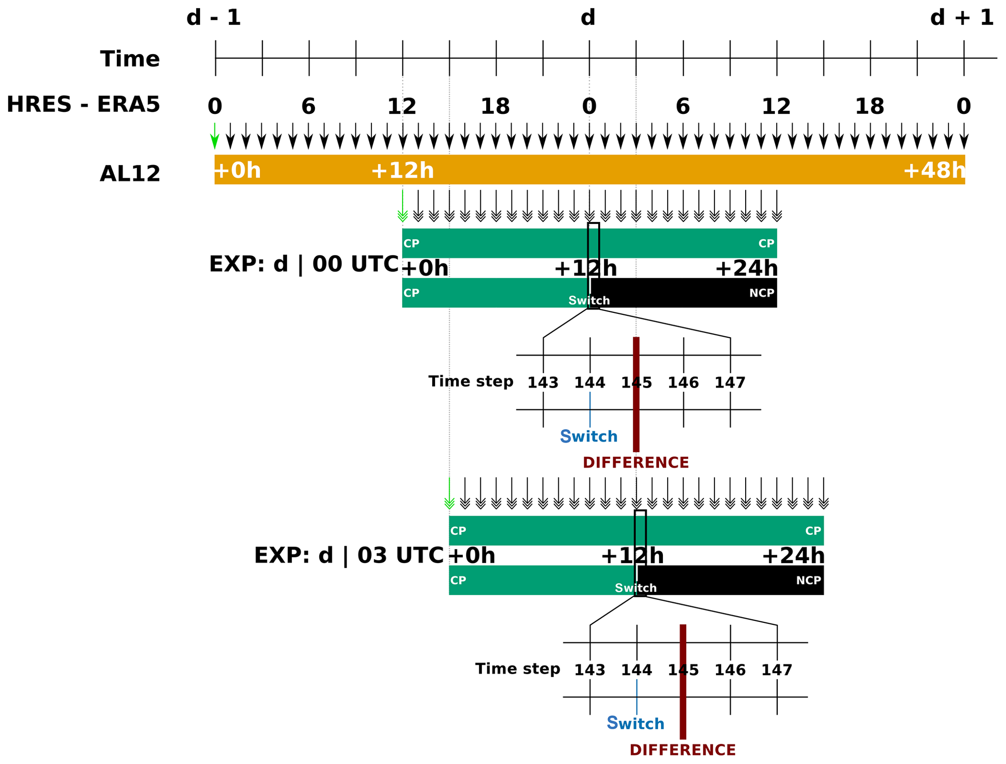
Figure 3 Organization of the different runs used to evaluate the flux differences. Both runs start with deep-convection parameterization (CP), while one of the forecasts switches off the parameterization after 12 h (NCP). Here an example is shown for evaluation of the transport flux error at 00:00 and 03:00 UTC. In practice such an evaluation is done every 3 h between 00:00 UTC on 2 April 2009 and 21:00 UTC on 10 April 2009. A green single arrows indicates initial conditions were provided by the ERA5 reanalysis, while a black single arrow means that the LAM was forced with ERA5 boundary conditions. Double arrows indicate initial and boundary conditions are provided from the 12 km intermediate simulation.

A schematic overview of the organization of simulations is given in Fig. 3. This figure shows the timeline for the model states of the HRES-ERA5 reanalysis for days d−1, d and d+1. These model states are provided with 1 h coupling-update frequencies (indicated with black single arrows) to the 12 km resolution version of the ALARO model (AL12) that is initialized at time d−1 and runs until 48 h lead time. The AL12 run is shown in yellow. These model states are then interpolated to the 4 km resolution domain to provide initial conditions and lateral boundary conditions for the 4 km runs (indicated with black double arrows). In the figure two such runs are shown in green; one at 12:00 and one at 15:00 UTC. As explained above we perform two 24 h parallel runs with this configuration, one with the deep-convection parameterization (CP) switched on for all lead times (indicated in green) and one where the deep-convection parameterization is switched off after a 12 h lead time, as indicated by the black line. Since both runs are exactly the same during the first 12 h (i.e. until time step 144 with a time step of 300 s), we ensure that model states are identical at that time, i.e. at 00:00 UTC on day d. At the next time step (i.e. time step 145 in the figure) we have two different model states which correspond to Eqs. (3) and (4). The errors are then computed by taking the difference as in Eqs. (7)–(9), and they are stored in a database. The same procedure is repeated for the whole time period of the experiment with 3 h time intervals. A second example at 15:00 UTC is shown below the first one in the figure.

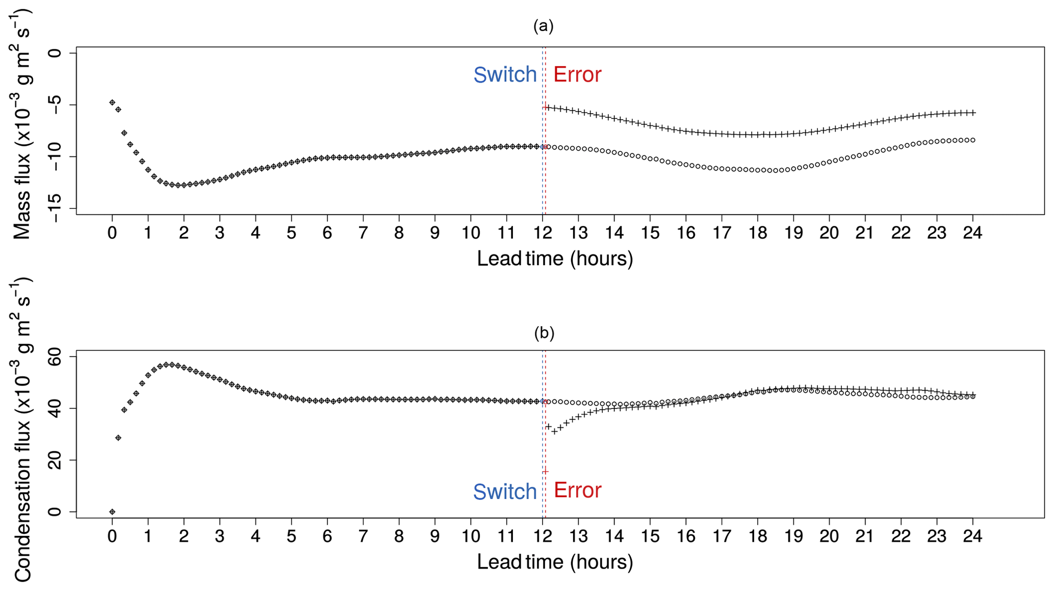
Figure 4 Domain averaged total transport fluxes,$J_{\mathrm{v}}^{\mathrm{td}}+J_{\mathrm{v}}^{\mathrm{c}}$ (open circles) and ${J^{\prime }}_{\mathrm{v}}^{\mathrm{td}}$ (crosses), for water vapour (a) and total condensation fluxes ($F_{\mathrm{vl}}^{\mathrm{st}}+F_{\mathrm{vl}}^{\mathrm{c}}$ and ${F^{\prime }}_{\mathrm{vl}}^{\mathrm{st}}$) for cloud water (b). Both forecasts are started at 12:00 UTC on 5 April 2009 with deep-convection parameterization; after 12 h (blue dashed vertical line) the deep-convection scheme is deactivated and both forecasts continue for another 12 h. The differences between the fluxes are diagnosed after one time step (red dashed vertical line).

Figure 4 shows the time series of the two 4 km runs for the domain-averaged water vapour transport flux and water vapour to cloud water condensation flux. During the first 12 h both forecast configurations are indeed identical. It can be seen that both the transport and condensation fluxes intensify (negative transport flux indicates upward transport) during the first 3–4 h spin-up period, before reaching a balanced state. The chosen moment at 12 h lead time for deactivating the deep-convection parameterization thus lies well outside of the spin-up regime.

The deactivation of the deep-convection parameterization leads to an instant increase in the domain-averaged water vapour transport flux due to the absence of a (mainly) upward convective transport (Fig. 4a). We see that the dynamics of the NCP model instantly take over some of the removed transport of the deep convective parameterization, and this leads to a difference that remains fairly constant between the NCP and the CP throughout the remainder of the two runs. The total transport flux difference one time step after the switch can be considered as a representative measurement of the error in the transport flux as defined in Eq. (7). Similar conclusions were found for the transport of the other species in Eq. (7) (not shown).

From Fig. 4b it can be seen that the resolved condensation in the microphysics parameterization starts to compensate for the absence of convective condensation with a negative jump at 12 h lead time. However, the NCP time series converges to the one of the CP run after 2 h. So the time series of the condensation flux does not suggest a model error after 2 h but instead we find that the NCP run is in an adjustment phase of the microphysics at the time step where we compute the model error. In this paper we will not investigate this issue in further detail but instead we will only study the errors for the transport fluxes ${\mathit{ϵ}}_{\mathit{\psi }}^{\mathrm{trans}}$ for $\mathit{\psi }=q_{\mathrm{v}},q_{\mathrm{l}},q_{\mathrm{i}},h,u,v$ in Eq. (7).

2.3 Properties of the vertical transport model error

In this section we discuss the most important properties of the model errors of the transport fluxes stored in the model error database.

2.3.1 Vertical profile

Figure 5 shows the average vertical profile of the transport flux errors of water vapour, enthalpy and zonal wind. The error in the water vapour transport flux (Fig. 5a) is positive (fluxes are counted negative upwards) at all levels but originates from different sources depending on the model level. The maximum error between 650 and 550 hPa corresponds to the underestimation of the upward transport of moist air when there is no deep-convection parameterization. The second smaller peak, around 950 hPa, is associated with the missing downdraft transporting drier air to the lower regions and results in an underestimation of the drying of the lowest levels when compared to simulations with deep-convection parameterization. Differences in the transport fluxes of the cloud condensates (not shown) display similar characteristics.

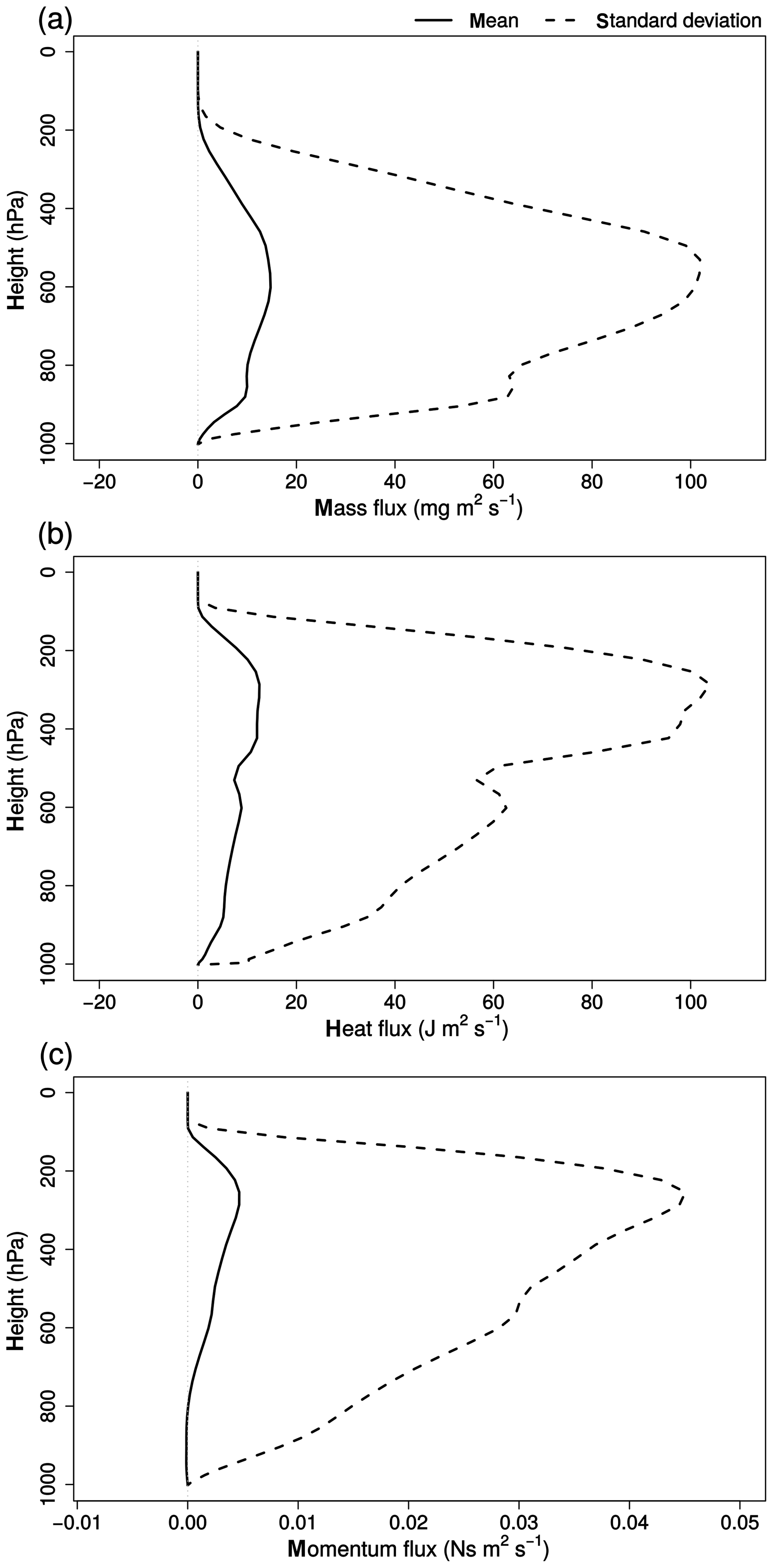
Figure 5 Vertical profile of the mean transport flux error (full line) and standard deviation (dashed line) for specific humidity (a), enthalpy (b) and zonal momentum (c).

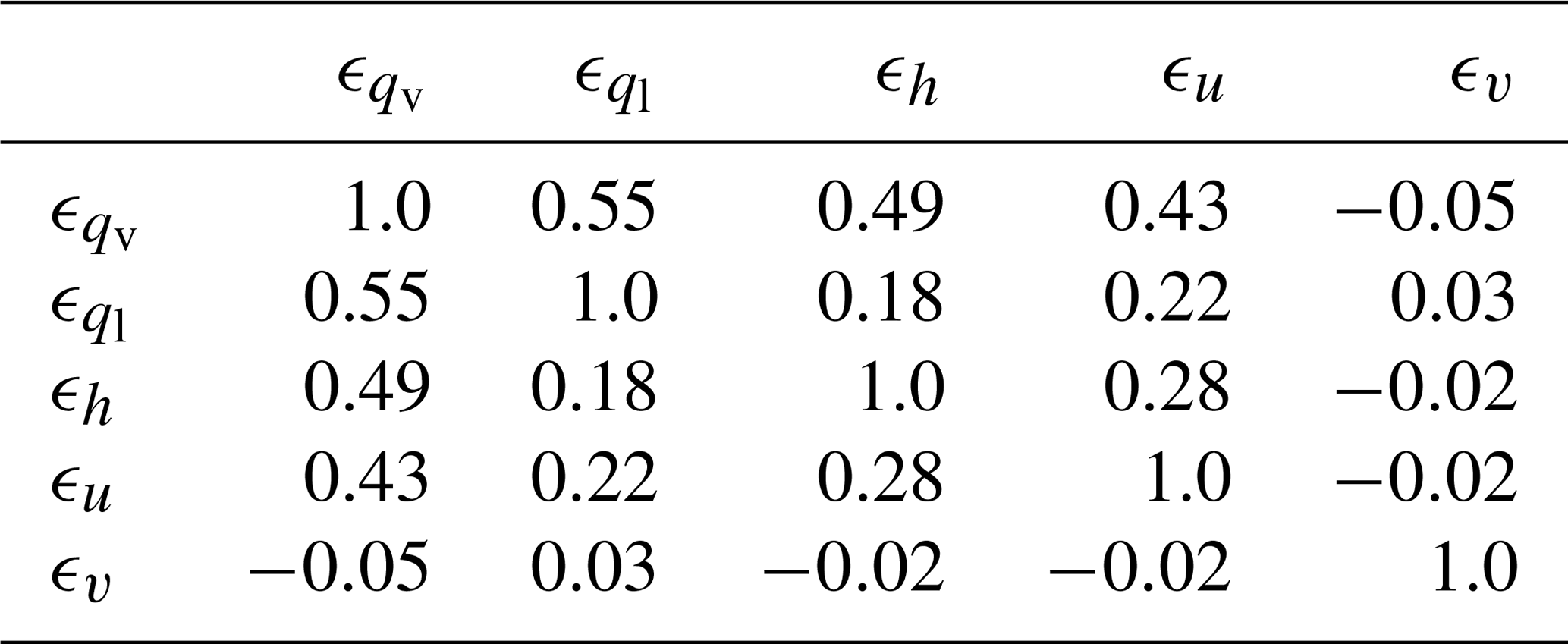
Table 1 Correlation matrix at model level 27 of the transport flux errors of water vapour (q_v), cloud water (q_l), enthalpy (h), and zonal (u) and meridional (v) wind.

Compared to water vapour, the error in enthalpy transport (Fig. 5b) peaks at a higher level (250–350 hPa). This peak is linked to the updraft parameterization, typically entraining warm air at its start and detraining it at higher levels. The reason the maximum transport flux error of water vapour lies at lower levels than that of enthalpy is explained by the condensation. At higher levels condensation removes some of the water vapour from the updraft, reducing its total transport. The smaller peak around 950 hPa in Fig. 5b coincides with that of Fig. 5a and is thus also linked to the downdraft transporting colder air down.

The interpretation of the transport flux error of zonal momentum Fig. 5c is somewhat counter-intuitive. Typically one would expect the error to be negative since the missing parameterized updraft transports air with lower momentum to higher levels where detrainment reduces the total momentum. The wind direction, however, is dominantly westward, resulting in a missing upward transport of slower, negative momentum and thus a positive error. At lower levels the downdraft transports high-momentum eastward (positive) wind downward, resulting in a (small) negative momentum flux error at 900–1000 hPa.

The standard deviations, shown in Fig. 5, are typically 1 order of magnitude larger than the mean of the respective errors. The convective transport is thus, besides being responsible for systematic forcing, also an important source of variability for the tendencies in the middle and upper troposphere.

2.3.2 Probability distribution

Figure 6 shows the probability density distribution of the flux errors at the level of highest variability (∼250 hPa) for water vapour, enthalpy and zonal momentum. All three distributions show a large peak around zero, indicating that in a majority of the grid points no error is present. This peak represents the grid points without any convective activity. The long tail of the distributions explains the large variance seen in Fig. 5. More specifically, the linear trend in the log-scaled figures for positive values, most distinct for water vapour and enthalpy, hints at an exponential distribution of the transport error in grid points with convective activity. The number of grid points with a negative transport flux error is very small (0.01 % and 1.8 % of the total amount of grid points with non-zero error for water vapour and enthalpy, respectively).

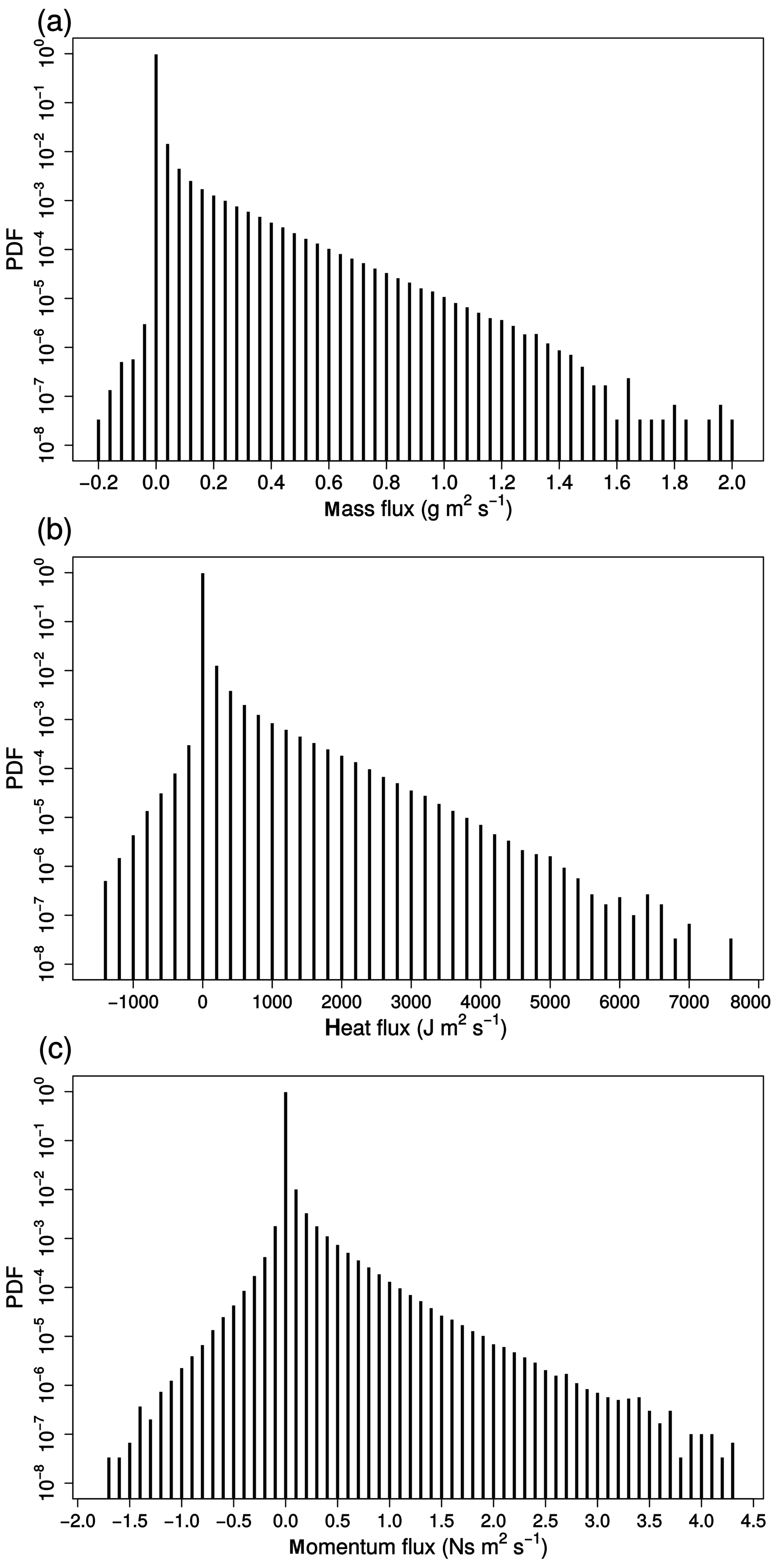
Figure 6 Probability density function (PDF) of the transport flux errors for water vapour (a), enthalpy (b) and zonal wind (c) at model level 20 (∼250 hPa).

2.3.3 Vertical correlation

The vertical autocorrelation of the water vapour, enthalpy and zonal wind transport flux errors is shown in Fig. 7. The correlation with vertically neighbouring grid cells is high for all three flux errors. The vertical correlation decays fastest for enthalpy, where the correlation drops below 0.2 after a distance of 75 hPa. Vertical correlation becomes negative for all errors for distances larger than 225 hPa. The vertical correlations indicate a clear vertical structure of the transport fluxes. Accounting correctly for this vertical structure is important when developing a stochastic perturbation scheme (see Sect. 3).

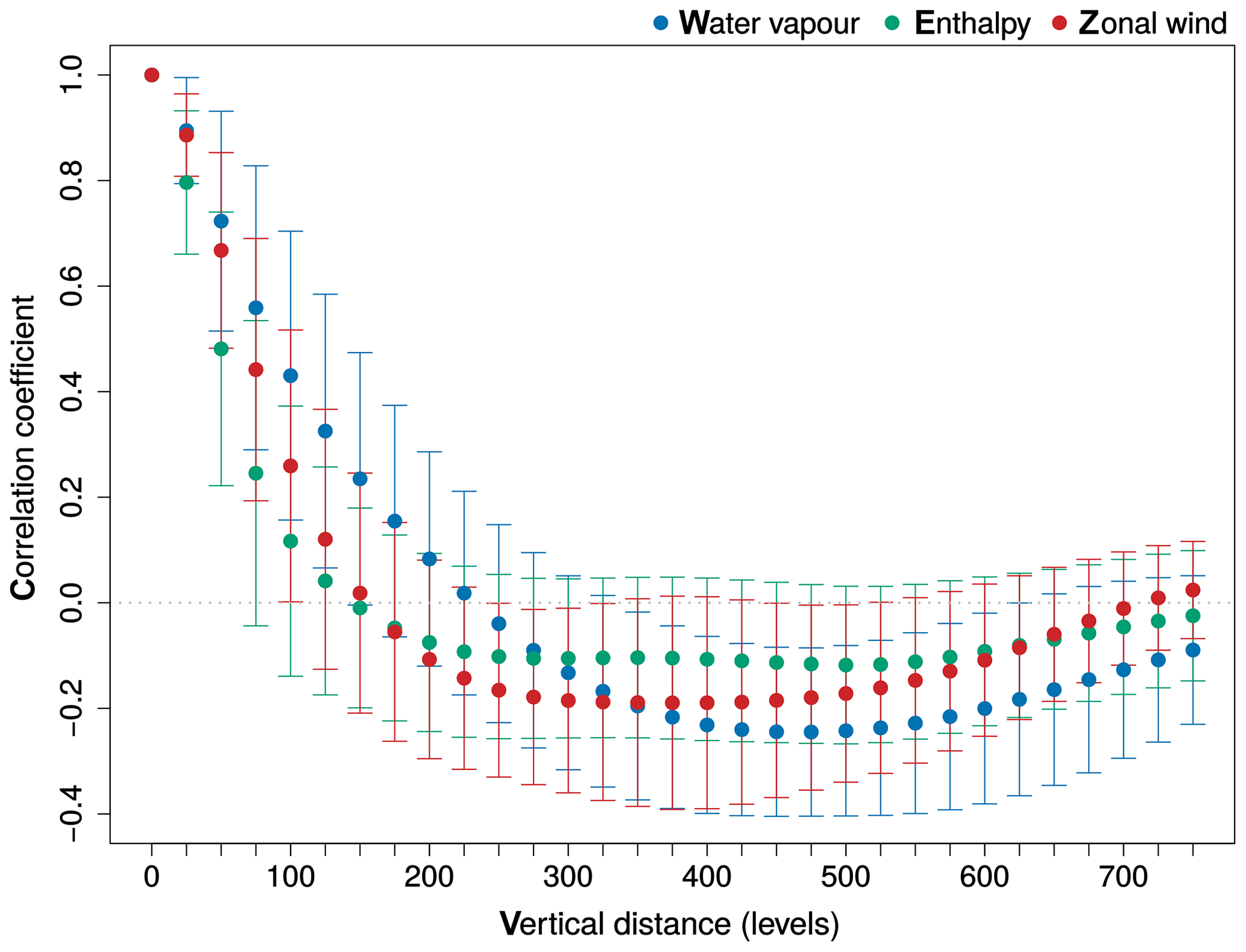
Figure 7 The vertical autocorrelation coefficients as a function of the vertical distance (in hPa) of the transport flux error for water vapour (blue), enthalpy (green) and zonal wind (red). The error bars show 1 standard deviation.

2.3.4 Inter-variable correlation

The transport flux errors of the different variables all originate from the absence of an up- and downdraft. Therefore, their inter-variable correlation is expected to be large. However, the correlation matrix (Table 1) shows only moderate correlation between water vapour, cloud water and zonal wind, while the correlation coefficient of the flux error of meridional wind with respect to the other errors is close to zero. This is because, contrary to the other variables, meridional momentum flux error does not have a dominant sign. For the same reasons as discussed for the vertical correlation, an appropriate representation of these inter-variable correlations should be a major requirement when building a stochastic perturbation scheme.

2.3.5 Correlation with transport flux

Finally the correlation of the errors with the total transport flux of the target model is investigated. Large correlation coefficients between the model transport flux and its error would suggest a linear relationship: ${\mathit{ϵ}}_{\mathit{\psi }}=a{J^{\prime }}_{\mathit{\psi }}^{\mathrm{trans}}{\mathrm{|}}_{\mathrm{unpert}}$. In this case the perturbed fluxes (${J^{\prime }}_{\mathit{\psi }}^{\mathrm{trans}}{\mathrm{|}}_{\mathrm{pert}}$) could be written in a multiplicative form, ${J^{\prime }}_{\mathit{\psi }}^{\mathrm{trans}}{\mathrm{|}}_{\mathrm{pert}}=(\mathrm{1}+a){J^{\prime }}_{\mathit{\psi }}^{\mathrm{trans}}{\mathrm{|}}_{\mathrm{unpert}}$, as is done in the SPPT scheme. Figure 8 shows the correlation between the transport flux and its error for water vapour, enthalpy and zonal wind for all model levels. In general, the relation between a flux and its corresponding error is weak, with correlation coefficients ranging from −0.1 to 0.3. This seems to suggest that a stochastic perturbation scheme based on a simple multiplication of the fluxes with a random number will ignore part of the actual variability seen in the reference configuration, resulting in an under-dispersive ensemble system.

Figure 8 The Pearson correlation coefficients of the transport flux error with respect to the total transport flux of water vapour (blue), enthalpy (green) and zonal wind (red) at all model levels. The error bars show the 95 % confidence interval.

3 Random perturbations for uncertainty forecasting

3.1 Perturbation scheme

When perturbing the transport fluxes during a forecast, the distribution of the perturbations is ideally the same as the distribution of the errors described in the previous section. Additionally, the perturbations should preserve the vertical, horizontal, temporal and inter-variable correlations of the errors. However, how to enforce all of these constraints simultaneously remains an open question, not only here but also in other schemes (Palmer et al., 2009). Here, a simple perturbation scheme is proposed that simulates the distributions appropriately (Fig. 6), while also preserving the vertical and inter-variable correlation of the errors. As discussed above, the correct representation of both the vertical and inter-variable correlation of the transport flux perturbations is necessary to keep the perturbed fluxes physically consistent.

The vertical and inter-variable correlation are preserved by organizing the flux-error profiles per grid column in the model error database, i.e. by grouping the vertical error profiles ${\mathit{ϵ}}_{\mathit{\psi }}^{\mathrm{trans}}$ for all species $\mathit{\psi }=q_{\mathrm{v}},q_{\mathrm{l}},q_{\mathrm{i}},h,u,v$ at a specific grid point and a specific time, always as one multivariate set. During the forecast, the transport fluxes inside a particular grid column are randomly perturbed by sampling a grid column from the model-error sets and subtracting the associated flux errors from the respective total fluxes (Fig. 9). The resulting perturbed tendencies can thus be written as

$$\begin{array}{}\text{(10)}& {\displaystyle \frac{\partial \mathit{\psi }}{\partial t}}{\mathrm{|}}_{\mathrm{pert}}=-g{\displaystyle \frac{\partial }{\partial p}}(J_{\mathit{\psi }}^{\mathrm{tot}}-{\mathit{ϵ}}_{\mathit{\psi }}^i),\end{array}$$

with all flux-error profiles ($\mathit{\psi }=q_{\mathrm{v}},q_{\mathrm{l}},q_{\mathrm{i}},h,u,v$) belonging to the same sampled grid column i. Adding the error as a flux in a flux-conservative manner in Eq. (10) ensures that the total budgets of mass and energy are conserved by the perturbation.

Figure 9 Schematic overview of the sampling of a grid column containing the different transport flux errors.

The distribution shown in Fig. 6 contains all grid columns, including those without any convective activity, resulting in a large number of cases where the flux error is zero. Since we only study model errors originating from the deep-convection scheme we will exclude these points from the model-error database. Only grid columns where the convective activity is significant are retained by defining a cut-off updraft mass flux M_cut-off and selecting only those grid columns which satisfy

$$\begin{array}{}\text{(11)}& \stackrel{\mathrm{‾}}{M_{\mathrm{u}}}<M_{\text{cut-off}}\mathrm{with}\stackrel{\mathrm{‾}}{M_{\mathrm{u}}},M_{\text{cut-off}}<\mathrm{0},\end{array}$$

with $\stackrel{\mathrm{‾}}{M_{\mathrm{u}}}$ the updraft mass flux, available from the CP configuration, averaged over the vertical column. This allows us to retain only the error at those grid columns where convective activity is relevant. This is achieved by taking a value of $M_{\text{cut-off}}=-\mathrm{0.5}$ Pa s⁻¹.

Finally, a proxy for deep convection is needed to determine the grid columns in the NCP run where the transport fluxes should be perturbed. Two different convection criteria are compared. The first criterion (labelled MOCON) uses the vertically integrated moisture convergence in the planetary boundary layer as a proxy for convective activity (Waldstreicher, 1989; Calas et al., 1998; van Zomeren and van Delden, 2007), while the second configuration (labelled OMEGA) uses the grid column averaged resolved vertical velocity. For both proxies a threshold value, MOCON_c and OMEGA_c respectively, is determined. During every time step of the integration, when the chosen threshold is exceeded for a given grid column, a sample is drawn from the database, as shown in Fig. 9, and the transport fluxes are perturbed according to Eq. (10). Although the perturbations are sampled independently in space and time from the database, the use of these thresholds introduces some crude spatio-temporal correlation in the flux perturbations.

The choice of the threshold criteria OMEGA_c and MOCON_c is closely related to the one of the cut-off updraft mass flux M_cut-off. While M_cut-off can be used to decide what part of the tail of the flux-difference distribution will be sampled from, OMEGA_c and MOCON_c are chosen such that the percentage of grid columns exceeding the threshold in the perturbed forecast is roughly equal to the percentage of grid columns selected on the basis of M_cut-off. With $M_{\text{cut-off}}=-\mathrm{0.5}$ Pa s⁻¹, OMEGA_c was set to −0.2 Pa s⁻¹, while MOCON_c was set to $\mathrm{4}\times {\mathrm{10}}^{-\mathrm{3}}$ g m⁻² s⁻¹.

3.2 Results and discussion

The above-described perturbation scheme has been tested with the ALARO model configuration without deep-convection parameterization to see whether a stochastic perturbation can compensate for the error due to the lack of the parameterization.

The runs were carried out for a 10 d period between 11 and 20 April 2009 over the same domain as described in Sect. 2.2. Every day a 10-member 48 h ensemble forecast is started at 00:00 UTC. Tests were carried out for both the hydrostatic and non-hydrostatic set-up of the ALARO model. Since conventional wisdom dictates that non-hydrostatic models should be applied at these resolutions we will only show here the results for the non-hydrostatic model configurations. The tests with the hydrostatic formulation (not shown) led to exactly the same conclusions.

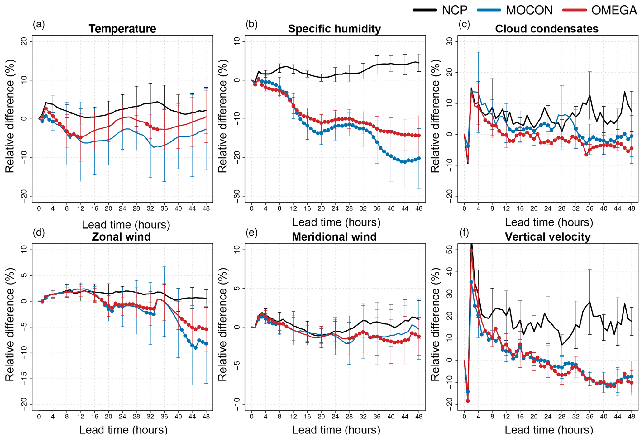
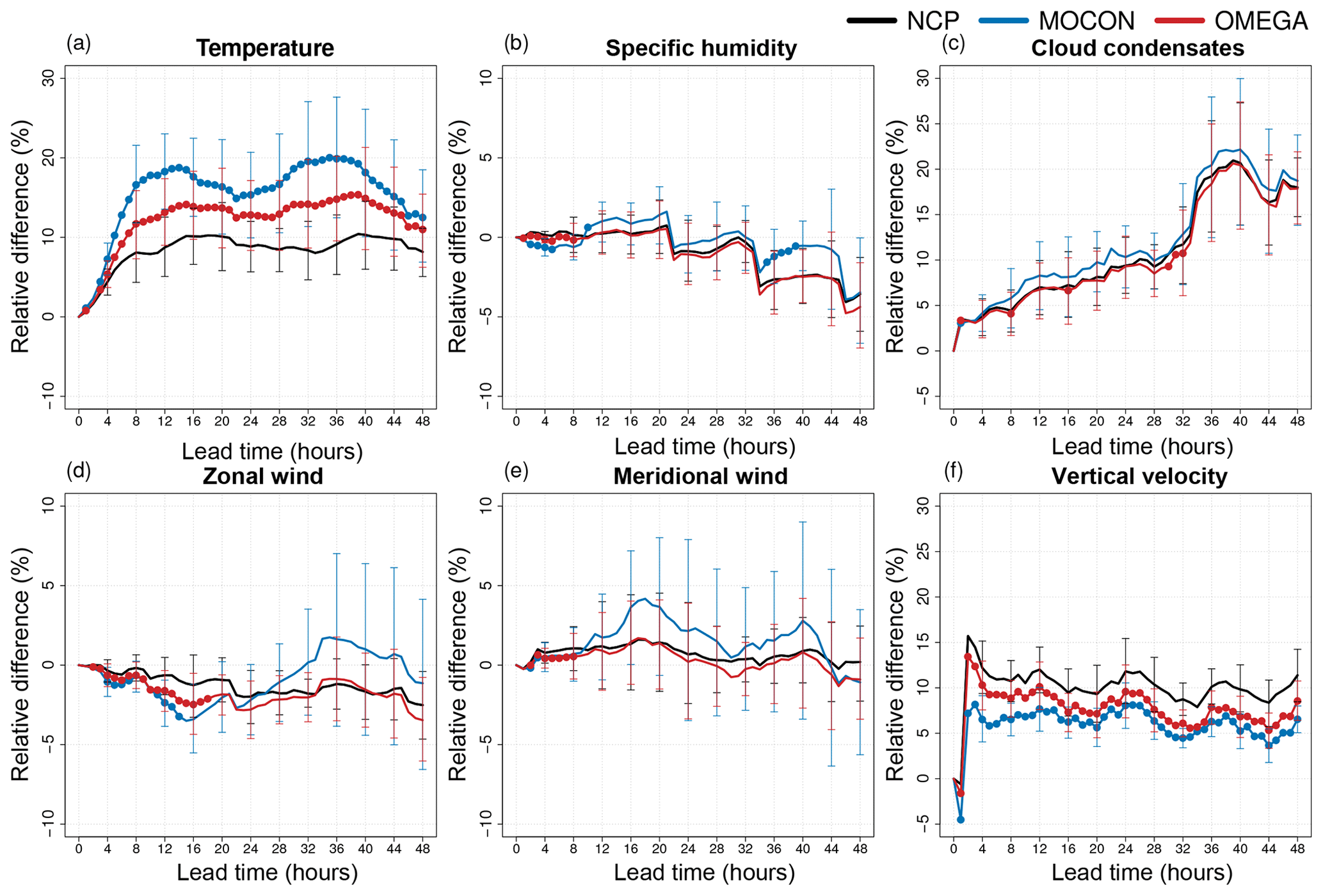
Figure 10 Relative RMSE difference (in percentage with respect to the CP configuration) of the NCP (black) control forecast (deterministic) and the MOCON (blue) and OMEGA (red) ensemble mean for temperature (a), specific humidity (b), cloud condensates (c), zonal (d) and meridional (e) wind, and vertical velocity (f) at 250 hPa. Both ensemble forecasts are performed without perturbations in ICs and LBCs. Error bars show the 95 % confidence interval. Lead times where the ensemble mean RMSE is significantly lower than the NCP control RMSE at the 95 % confidence level are indicated with a filled circle.

3.2.1 No IC and LCB perturbations

The direct impact of the stochastic forcing is studied by running both ensemble configurations MOCON and OMEGA without IC and LBC perturbations and comparing the RMSE of the ensemble mean (with respect to the ERA5 HRES analysis) and the RMSE of the deterministic NCP (target) forecast with that of the deterministic CP (reference) forecast. The scores are defined in Appendix B.

The impact is largest in the upper atmosphere (Fig. 10). Here the RMSE of the ensemble mean of both ensemble configurations is significantly better than the NCP configuration for most of the variables and lead times. The OMEGA configuration only performs better than the CP configuration for specific humidity (all lead times) and vertical velocity (after 24 h).

This means that perturbing with flux errors indeed compensates the error made by disabling the deep-convection parameterization, as was the immediate goal of these perturbations. But even better, part of the error in the reference configuration due to the stochastic nature of deep convection, is correctly captured by the flux-error perturbation scheme.

Figure 11 Same as Fig. 10 but for the 850 hPa level.

In the lower atmosphere (Fig. 11) the effect of the stochastic perturbations is smaller. Here, the forcings have no significant impact on the temperature RMSE and also the reduction in specific humidity error is smaller, albeit still significant. This is explained by looking back at profiles of flux differences in Fig. 5a and b. At 850 hPa the mean tendency perturbations caused by the addition of the corrective flux profiles is close to zero for both specific humidity and temperature, while the standard variation of the corrective fluxes is also smaller here than aloft. The situation for cloud condensates is opposite, with a small but significant improvement in RMSE at the 250 hPa level and quite a large improvement below at the 850 hPa level.

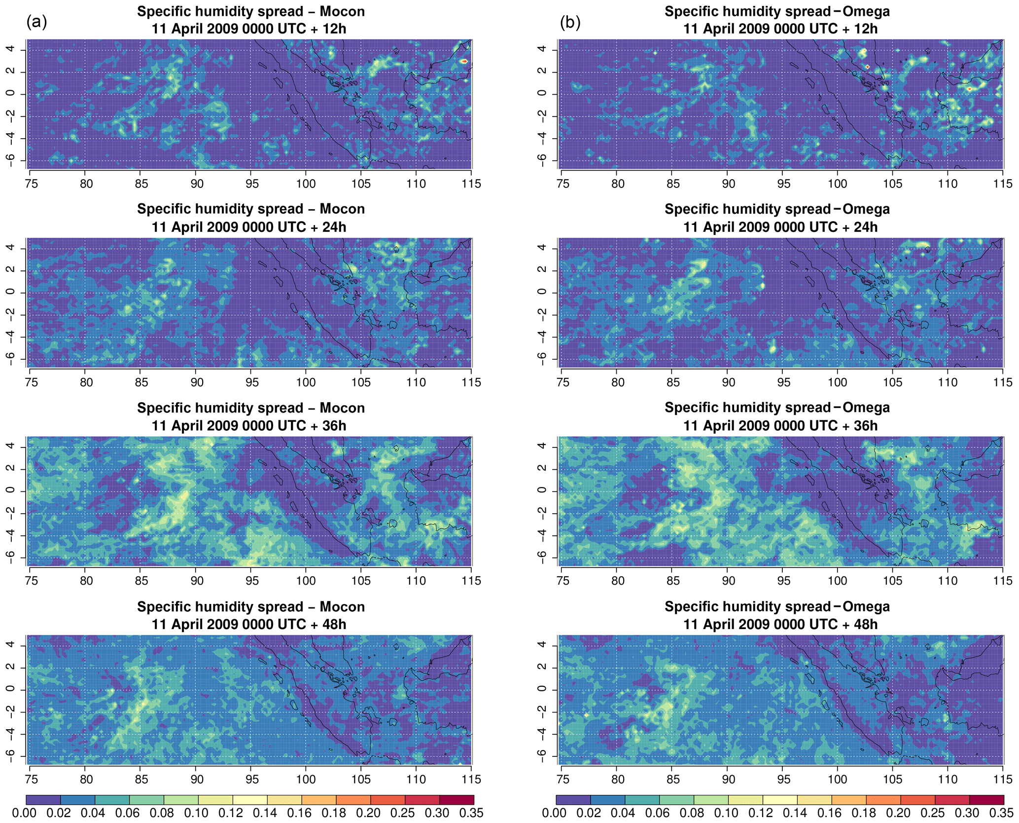
Figure 12 Snapshots of the specific humidity spread (g kg⁻¹) at 250 hPa for the MOCON (a) and OMEGA (b) ensemble without perturbations in ICs and LBCs. Snapshots are shown for every 12 h during the 48 h forecast started at 00:00 UTC on 11 April 2009.

Figure 12 shows the spread created by the stochastic forcing from both perturbation configurations for specific humidity at 250 hPa at different lead times. The two ensemble configurations create similar spread both in amplitude and in spatial distribution, with the largest spread concentrated in regions with convective activity. While the spread does show some spatial growth during the first 24 h, the impact of the stochastic perturbations remains limited for regions with no convective activity. Furthermore, the spread created during a convective episode does not seem to continue to grow once the convective episode is over and there is no longer a stochastic contribution to the tendencies. This is seen for instance over the Java Sea between Java and Borneo, where the spread induced after 24 h has almost disappeared 24 h later.

These results clearly show that the proposed stochastic scheme provides a sensible way to generate perturbations. The effect of the stochastic perturbations is twofold. First of all they force the individual members closer to the CP forecast, reducing the error. This is a logical consequence of perturbing the members by sampling the flux differences between target and reference forecasts. On top of that, the spread is created at locations consistent with the error of the reference configuration, resulting in an ensemble that is more skillful than the reference CP forecast.

Figure 13 Ensemble spread of the MOCON (blue) and OMEGA (red) ensemble with (full lines) and without (dashed lines) IC and LBC perturbations together with the NCP (black) and CP (green) ensemble spread (created only by IC and LCB perturbations) at 250 hPa. Spread is calculated for temperature (a), specific humidity (b), cloud condensates (c), zonal (d) and meridional (e) wind, and vertical velocity (f).

3.2.2 IC and LBC perturbations

Next, the interaction of the stochastic forcing with the IC and LBC perturbations is studied. The impact on the ensemble spread at 250 hPa is shown in Fig. 13. In general the spread created by the stochastic forcing alone is much smaller (between 40 % and 60 %) than that created by the perturbed initial and boundary conditions. For only cloud condensates and vertical velocity, the spread induced by stochastic forcing alone approaches the spread generated by the perturbed initial and boundary conditions. The figure also shows that the combined effect of physics and IC/BC perturbations is smaller than the sum of the individual effects. This is in agreement with the findings of Baker et al. (2014) and Gebhardt et al. (2011).

For all variables the spread of the CP ensemble is smaller than that of the NCP ensemble. Comparing the snapshots of the zonal wind spread at 250 hPa of CP and NCP at 00:00 UTC on 13 April 2009 (+48 h) (Fig. 14) shows a similar pattern of large-scale variability. The higher domain-averaged spread of the NCP ensemble is (dominantly) caused by increased small-scale variability. This small-scale variability is linked to regions with excessive updrafts resulting from the absence of a subgrid stabilizing mechanism. It is, however, questionable that an increase in spread resulting from an inadequate representation of a certain process is an appropriate way to increase the skill of an ensemble.

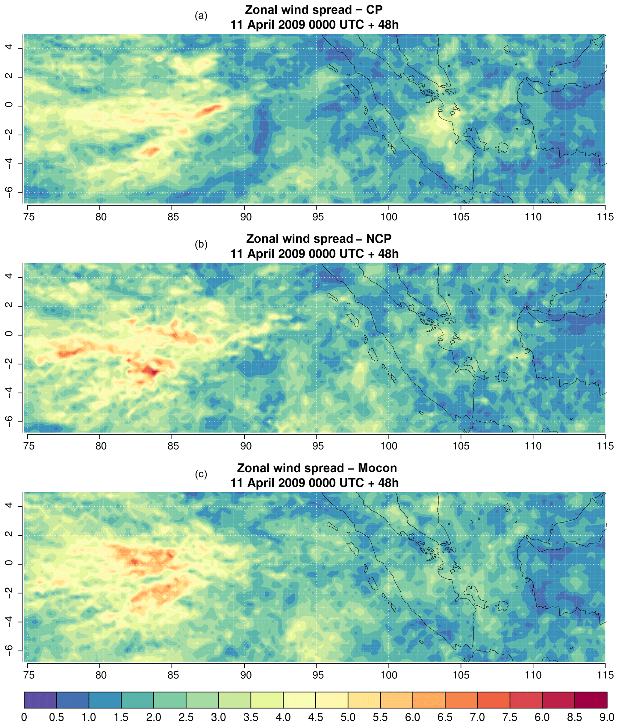
Figure 14 Snapshot of the zonal wind spread (m s⁻¹) at 250 hPa. Snapshot is taken at verification date 00:00 UTC on 13 April 2009 (lead time 48 h) for the CP (a), NCP (b) and MOCON (c) ensembles, all with IC and LBC perturbations.

The addition of the stochastic perturbations increases the spread (between 4.9 % and 8.6 % with respect to the NCP ensemble) for all variables at 250 hPa except specific humidity. Figure 14c shows that the increased spread is mainly caused by an expansion of regions with moderate spread (e.g. around 95^∘ E), while regions of high spread now show a smoother pattern thanks to the introduced stabilizing fluxes. This is true especially for the specific humidity (not shown), where a decrease in spread is combined with a large increase in skill (Fig. 15b). Here the stabilizing flux perturbations reduce the (erroneous) spread while still maintaining enough small-scale spread, resulting in substantial increase in skill.

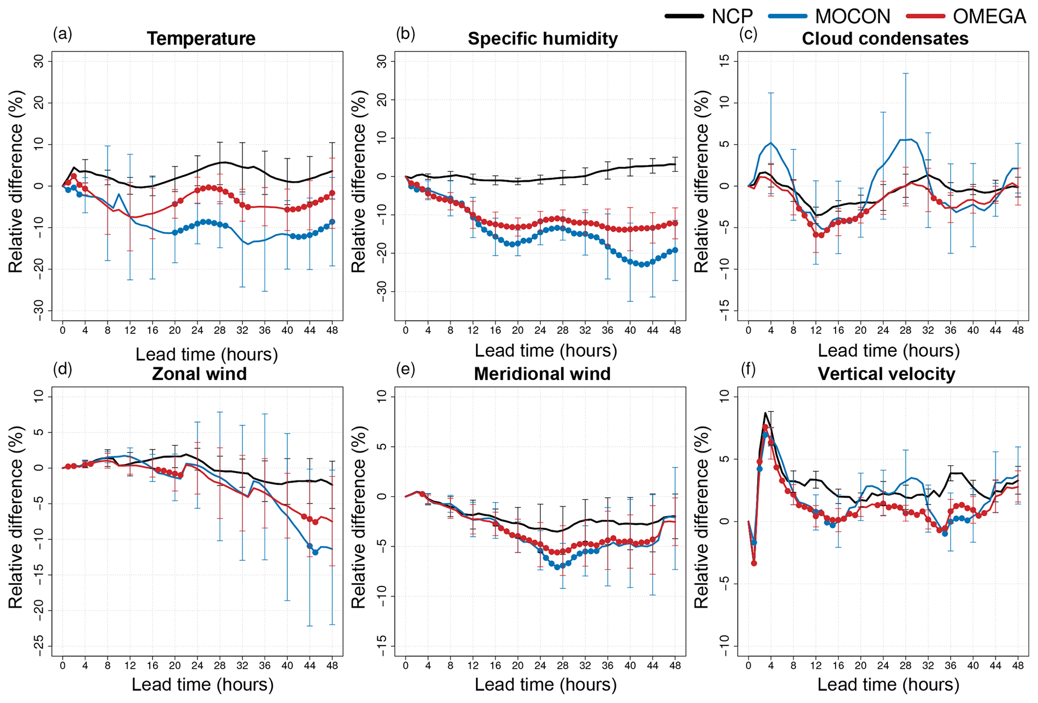
Figure 15 CRPS of the NCP (black), MOCON (blue) and OMEGA (red) ensemble for temperature (a), specific humidity (b), cloud condensates (c), zonal (d) and meridional (e) wind, and vertical velocity (f) at 250 hPa. All ensemble forecasts are performed with perturbations in ICs and LBCs. Error bars show the 95 % confidence interval. Lead times where the ensemble mean RMSE is significantly lower than the NCP control RMSE at the 95 % confidence level are indicated with a filled circle.

Figure 16 Same as Fig. 15 but for the 850 hPa level.

The impact of the flux perturbations on the probabilistic skill is analysed on the basis of the continuous ranked probability score (CRPS) calculated against the ERA5 HRES analysis. Figures 15 and 16 show the relative difference in CRPS of the NCP, MOCON and OMEGA ensemble with respect to the CP ensemble for the upper and lower atmosphere, respectively. The impact of the stochastic forcing is highest in the upper atmosphere. As mentioned above, the best results are seen for temperature and specific humidity, with significant improvements in specific humidity CRPS up to 24 % and 13 % for the MOCON and OMEGA ensembles respectively with respect to the CP reference ensemble and up to 31 % and 20 % with respect to the NCP target ensemble. The impact of the flux perturbations is less pronounced for the other variables, with smaller or non-significant improvements with respect to the NCP configuration.

Considering the spread in Fig. 15, for horizontal wind, one can see that the CP reference ensemble performs worse than the target NCP ensemble after 22 (4) h for the zonal (meridional) component. This is probably due to the smaller spread of the reference ensemble compared to that of the target ensemble (see Fig. 13) as explained above. Finally, for cloud condensates and vertical velocity the difference between the target NCP and reference CP ensemble is small and also the impact of the stochastic forcings is limited, with the CRPS of the MOCON and OMEGA ensemble lying below the CP scores or between the NCP and CP ones, respectively. It seems that the spread created by the initial and boundary condition perturbations partly reduces the improved skill of the CP configuration seen in Fig. 10.

At 850 hPa (Fig. 16), the most notable changes in CRPS scores are found in temperature, zonal wind and vertical velocity. Zonal wind scores of the MOCON ensemble have significantly improved with respect to both the NCP and CP ensembles, while the vertical velocity has improved with respect to the NCP ensemble only. Changes in 850 hPa temperature due to the stochastic forcing are up to 11 % and 5 % worse for the MOCON and OMEGA ensemble, respectively. Differences in specific humidity and meridional wind scores between the NCP and CP ensembles are small, and also the impact of stochastic forcings is mostly neutral.

For the upper-troposphere zonal wind, the improvements (9 %) in skill are substantial when compared to other state-of-the-art stochastic perturbation schemes. In Ollinaho et al. (2017) improvements by the SPP and SPPT scheme around 2.5 % are reported for zonal wind at 200 hPa. For 850 hPa zonal wind CRPS improvements induced by the SPP and SPPT scheme (1.8 %) are also comparable to the results presented here (1.7 %). The RP scheme presented in Baker et al. (2014) has a slightly larger impact, with improvements around 15 % and 10 % for 1.5 m temperature and humidity, respectively. However, one should keep in mind that only perturbations related to deep convection are considered here, while the SPP (RP) scheme perturbs 20 (16) parameters including turbulent diffusion, convection, cloud processes and radiation.

Table 2 Relative difference as percentage (with respect to the NCP configuration) in the number of times the ERA5 HRES reanalysis lies inside the range of the ensemble at lead time 48 h for specific humidity, temperature and zonal wind. Values that are significant at the 95 % confidence interval are highlighted in bold.

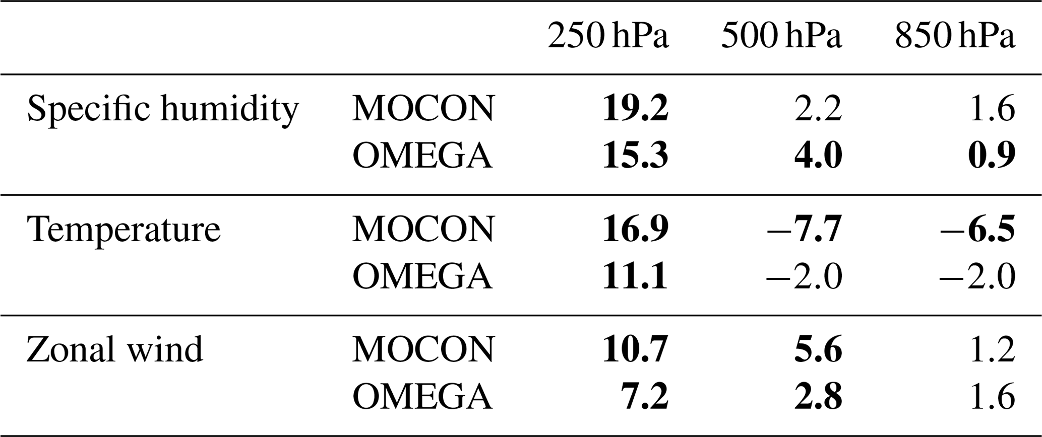
Finally, the relative change in dispersion of the MOCON and OMEGA ensembles is investigated with respect to the NCP ensemble. Table 2 shows the relative difference (as a percentage) in the number of times the ERA5 HRES reanalysis lies inside the range of the ensemble at lead time 48 h. For all configurations the ensemble is under-dispersive, a characteristic common to all single-model ensembles (Palmer et al., 2005). In the upper atmosphere (250 hPa) the flux perturbation reduces the under-dispersion for all variables. At this level the increase in number of observations falling within the ensemble is the result of a reduction in the bias of the individual ensemble members (not shown) and an increase in the spread. In the middle (500 hPa) and lower (850 hPa) atmosphere, under-dispersion is reduced for water vapour and zonal wind, while the stochastic ensembles are more under-dispersive for temperature. The flux perturbations have little influence on the spread in the lower atmosphere (not shown). Therefore, changes in dispersion are mainly attributed to the positive (negative) shift in ensemble bias for specific humidity and zonal wind (temperature).

3.2.3 Precipitation

In what follows, the results for the OMEGA ensemble are very similar to those of the MOCON ensemble and are omitted for clarity. The ensemble skill for precipitation was evaluated using the CRPS calculated for the 3-hourly averaged precipitation with respect to the TRMM observations. The CRPS of all ensembles correlates well with the convective diurnal cycle (not shown). During a full day the 3-hourly averaged precipitation reaches a maximum at 09:00 UTC (around 16:00 local time) with a second smaller peak at 21:00 UTC (04:00 local time) (not shown). The peaks in CRPS at lead times 9, 21 and 33 h are closely linked to these maxima of precipitation. Investigation of the domain-averaged precipitation amounts (not shown) reveals that the absolute error in domain-averaged precipitation is constant throughout the day, meaning that the diurnal pattern in the CRPS is caused by a mismatch of local precipitation regions rather than by an overall misrepresentation of the convective diurnal cycle.

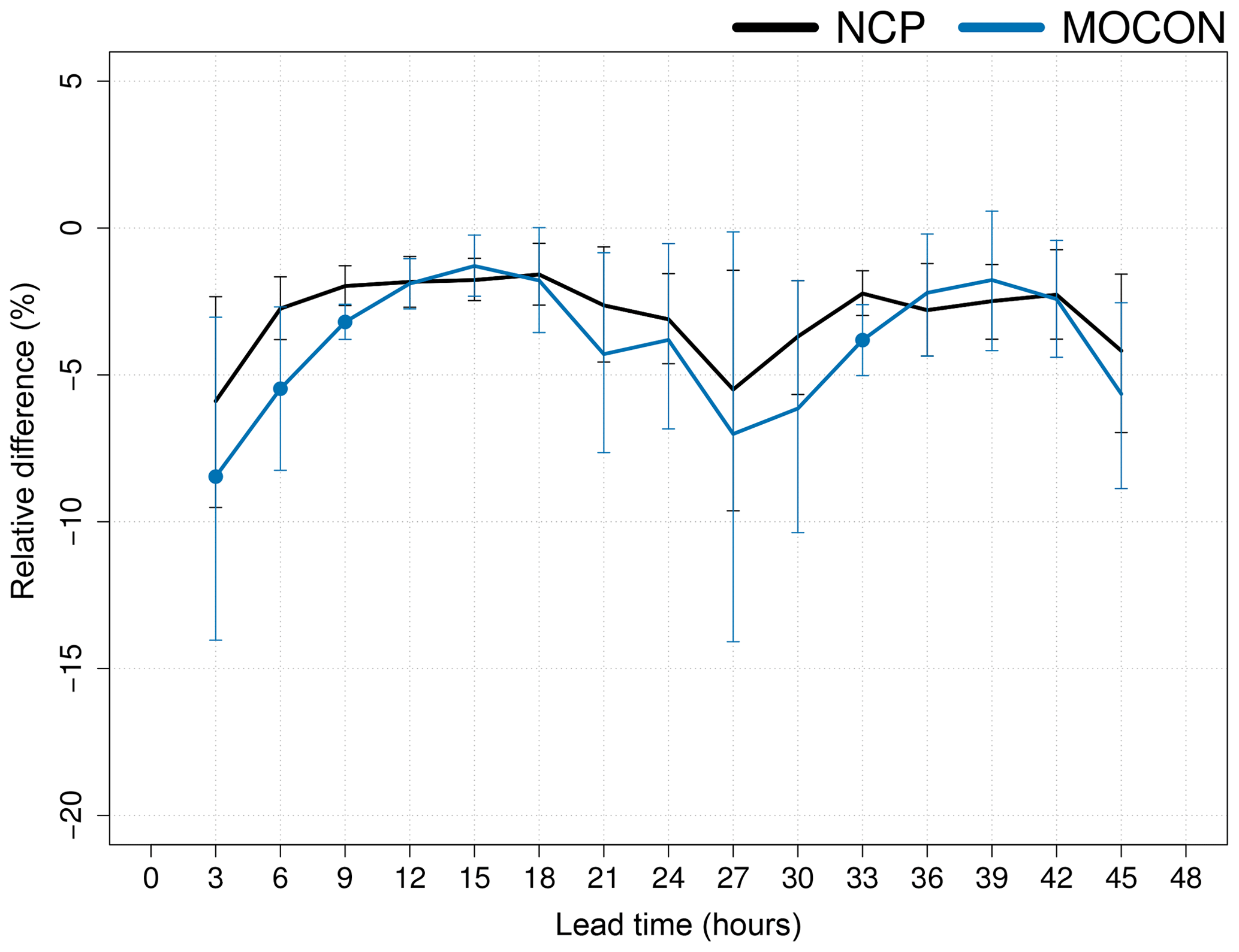
Figure 17 Relative change in precipitation CRPS with respect to the CP ensemble of 3-hourly averaged precipitation for the NCP (black) and MOCON (blue) ensemble. All ensembles include IC and LBC perturbations. The error bars show the 95 % confidence interval. Lead times where the CRPS of MOCON is significantly different from that of NCP are indicated with filled circles. The CRPS is calculated with respect to TRMM observations.

Figure 17 shows the relative change in CRPS with respect to the CP ensemble. The impact of the absence of a deep-convection parameterization and stochastic forcing on the 3-hourly averaged precipitation is relatively small.

There is a neutral to positive impact in skill for the MOCON ensemble (albeit inside the significance confidence intervals). This is an improvement compared to Baker et al. (2014), who only found improved skill in the precipitation rate during the first 2 h with their RP scheme and a worsening afterwards. A significant improvement in CRPS is also seen at lead time 33 h, coinciding with a maximum in convective activity. Unsurprisingly, the convective activity must be high in order for the stochastic forcing to have a significant effect on the precipitation.

In order to differentiate between different precipitation regimes, the Brier skill score (BSS) with respect to the CP ensemble for 24 h cumulated precipitation is shown in Fig. 18 for different thresholds. A significant difference between the NCP and MOCON ensemble is only seen at low thresholds (1 and 5 mm d⁻¹). At these low precipitation thresholds, the perturbations bring the precipitation distribution of the MOCON ensemble closer to that of the reference CP ensemble. Figure 18 also shows that the NCP ensemble performs significantly better than the CP ensemble at the these low thresholds. It seems that for low precipitation rates, the consistency between the different members of the CP configuration (a result of the deep-convection parameterization) is penalized. The spread created by local grid point storms, on the other hand, is rewarded in the setting of an ensemble forecast. This result can be attributed to the same syndrome of better scores for the wrong reasons, as discussed in Sect. 3.2.2. At larger thresholds no significant difference in BSS between the CP and both NCP and MOCON configurations is found. These results further confirm the suggestion that the transport fluxes from the deep-convection scheme have a limited impact on the precipitation amounts.

Figure 18 The Brier skill score with respect to the CP ensemble of the NCP (black) and MOCON (blue) ensemble for 24 h accumulated precipitation at different thresholds. The Brier score is calculated with respect to TRMM observations. The error bars show the 95 % confidence interval. Filled circles show where the MOCON BSS is significantly different from the NCP BSS.

3.3 Time to solution

Finally, the computing performance of the different configurations is studied. To this end, the time to solution of a single 48 h forecast was measured for all configurations. The reference CP configuration has the longest time to solution (2213.71 s; on 4 CPUs with 24 cores, Intel Xeon EP E5-2695 V4). The deep-convection parameterization has a large impact on the run time. Deactivating it shortens the run time by almost 12 %. Both stochastic configurations have a small impact on the time to solution. With an increase in run time of 1.24 % with respect to the NCP configuration, the MOCON configuration has the fastest time to solution (between CP, MOCON and OMEGA). Most (1.04 % of the total run time) of the extra run time is spent selecting the active grid columns and adding the fluxes. Loading the flux-difference database only occupies a small fraction of the extra run time (0.03 % of the total run time) but does consume around 30 % more memory. Relative to the NCP configuration the OMEGA forecast is 1.36 % slower. The added time with respect to the MOCON configuration stems from additional calculations needed to diagnose the column-averaged vertical velocity.

4 Conclusion and outlook

This paper presents a novel approach for perturbing physics parameterizations of numerical weather prediction systems. The novelty lies in the idea that the perturbations are sampled from a database of model error estimates. In particular, the model errors studied here originate from switching off the parameterization of deep convection, thus degrading the forecast skill. The error is then diagnosed by taking the difference of the contributing physics fluxes of the runs with and without parameterization. Analysis of the error fluxes reveals the importance of the vertical correlation structure, as well as of the inter-variable correlation. Next, it is investigated whether these stochastic flux perturbations can increase the probabilistic forecast skill in an ensemble context in such a way that it compensates for the lack of parameterization.

The sampling method was implemented in a 10-member ensemble system testbed driven by the members of the ERA5 analysis. From the tests it has been shown that the ensemble system with the stochastic perturbations along with the IC and LBC perturbations compensates for the absence of the parameterization scheme.

The ensemble without the deep-convection parameterization exhibits too much spread as a result of inadequate representation of the convective processes at the convection-permitting scales. The introduction of the stochastic perturbations has a stabilizing effect on the convective adjustment and reduces this small-scale erroneous spread while increasing the overall spread (except for specific humidity), leading to a more skillful ensemble. The impact is largest in the upper troposphere with significant improvements in forecast skill for temperature, specific humidity and both zonal and meridional wind. At 850 hPa, improvements are smaller or neutral, except for temperature where the forecast skill is degraded.

An increasing number of ensemble prediction systems are now entering the convection-permitting scales (4–1 km). Most of them are based on the assumption that deep convection is explicitly resolved (e.g. Gebhardt et al., 2008; Schwartz et al., 2010), even though the threshold resolution for turning off the deep convective parameterization is not well established. It may be advocated (see for example Yano et al., 2018) that the transition towards fully convection-resolved resolutions should be carried out gradually. The stochastic perturbation approach presented here could be seen as such an intermediate approach avoiding the application of a scale-aware parameterization while still dealing with the ensuing model errors in a probabilistic sense.

The results shown here were produced in a controlled testbed, relying on perfect boundary conditions from the ERA5 reanalysis. To be able to optimally exploit the features of this approach within an operational EPS system it would be helpful to address a few issues.

For instance, a better understanding of the strong moisture readjustment regime after disabling the deep-convection parameterization within the error-diagnostics procedure could be useful. An investigation could be made into how to estimate the condensation flux differences by protecting the convective condensates from re-evaporation after disabling the deep-convection scheme. If a controlled adjustment could be developed then the errors in the condensation and evaporation fluxes might also be taken into account in the stochastic perturbation, potentially leading to a higher probabilistic forecast skill.

Combining the vertical correlation and multivariate correlation between the different flux perturbations with adequate spatio-temporal correlations would be useful, possibly relying on principle component analysis methods. In addition, the definition of the conditions determining the convective activity of a grid column and triggering the perturbations might be improved following the suggestions made in Banacos and Schultz (2005).

The creation of the sampling database requires extra implementation efforts and maintenance in an operational context. Additional research could be useful to model the error statistics and to find some universal error functions that may become candidates for PDFs to draw from for the stochastic sampling. The distributions found in Fig. 6 provide a good starting point for fitting such curves. If the functions are parameterized with a few parameters, the cumbersome computing task for estimating the error statistics may be replaced by a tuning exercise. Also the demanding task of building and maintaining the sampling database would not be necessary.

In Subramanian and Palmer (2017) the work on stochastic tropical convection parameterization done by Khouider et al. (2010), Frenkel et al. (2012) and Deng et al. (2015) is used in an ensemble context and the probabilistic features of the so-called ensemble super-parameterization are compared to those of a classical SPPT approach. It would be useful to extend their comparison with the approach suggested here. The process-oriented perturbation method, studied in this work, is indicated as highly desirable in Leutbecher et al. (2017) and is complementary to the different representations of model uncertainty presented in the introduction.

Appendix A: The ALARO model parameterization schemes

The ALARO model, used in this study, uses the “p-TKE” scheme for the parameterization of the boundary layer mixing. This scheme complements the method described in Louis (1979) by a prognostic equation for the total kinetic energy (TKE) (Geleyn et al., 2006). Shallow convection is part of the turbulence scheme through a modification of the Richardson number (Ri) as described in Geleyn (1986). The ALARO model can be run with and without parameterized deep convection. In the case of parameterized convection, the scale-aware 3MT scheme of Gerard et al. (2009) is used. This scheme calculates vertical transport fluxes as well as condensation fluxes, which contribute to the gross cloud condensates passed to the microphysical scheme. The microphysical processes are parameterized similarly to those in the scheme described in Lopez (2002), while a statistical sedimentation formalism proposed by Geleyn et al. (2008) is used to calculate the precipitation and sedimentation fluxes.

The coupling between physics and dynamics is handled by an interface based on a flux-conservative formulation developed in Catry et al. (2007) and further generalized in Degrauwe et al. (2016). The interface transforms the fluxes coming from the parameterizations to tendencies using a clean description of the thermodynamic and continuity equations, ensuring the conservation of heat, mass and momentum.

Appendix B: Forecast skill

Evaluating the impact on the forecast skill of the stochastic forcing in the absence of perturbations in initial and boundary conditions is done on the basis of root mean square error (RMSE) and ensemble spread. Root mean square errors are calculated with respect to the ERA5 HRES reanalysis:

$$\begin{array}{c}{\displaystyle }{\mathrm{RMSE}}_{\mathrm{ctrl}}=\sqrt{{\displaystyle \frac{\mathrm{1}}{nx\times ny}}\sum _{i,j=\mathrm{1}}^{nx,ny}(x_{i,j}^{\mathrm{ctrl}}-x_{i,j}^{\mathrm{era}}{)}^{\mathrm{2}}},\\ {\displaystyle }{\mathrm{RMSE}}_{\mathrm{stoch}}=\sqrt{{\displaystyle \frac{\mathrm{1}}{nx\times ny}}\sum _{i,j=\mathrm{1}}^{nx,ny}(\stackrel{\mathrm{‾}}{x_{i,j}^{\mathrm{stoch}}}-x_{i,j}^{\mathrm{era}}{)}^{\mathrm{2}}},\end{array}$$

where $x_{i,j}^{\mathrm{era}}$ and $x_{i,j}^{\mathrm{ctrl}}$ are the respective reanalysis and control (CP and NCP) forecast values of field x at grid point (i, j), $\stackrel{\mathrm{‾}}{x_{i,j}^{\mathrm{stoch}}}$ is the ensemble (MOCON and OMEGA) mean of field x at grid point (i, j), and nx and ny are the number of grid points in the x and y direction, respectively.

The spread of the ensemble created by the stochastic forcing is given by

$${\mathrm{spread}}^{\mathrm{stoch}}={\displaystyle \frac{\mathrm{1}}{nx\times ny}}\sum _{i,j=\mathrm{1}}^{nx,ny}{\mathit{\sigma }}_{xi,j}^{\mathrm{stoch}},$$

where

$${\mathit{\sigma }}_{xi,j}^{\mathrm{stoch}}=\sqrt{{\displaystyle \frac{\mathrm{1}}{n-\mathrm{1}}}\sum _{k=\mathrm{1}}^n{\left(x_{i,j,k}^{\mathrm{stoch}}-\stackrel{\mathrm{‾}}{x_{i,j}^{\mathrm{stoch}}}\right)}^{\mathrm{2}}}.$$

The impact of introducing the stochastic forcing together with perturbed initial and boundary conditions on the skill is expressed using the CRPS (Brown, 1974; Matheson and Winkler, 1976). The CRPS in point (i, j) measures the distance between the probabilistic forecast ρ of variable x and the reanalysis value x_era as

$${\mathrm{CRPS}}_{i,j}=\underset{-\mathrm{\infty }}{\overset{+\mathrm{\infty }}{\int }}{\left(P\left(x_{i,j}\right)-P_{\mathrm{era}}\left(x_{i,j}\right)\right)}^{\mathrm{2}}\mathrm{d}x,$$

with P(x) and P_era(x) cumulative distributions:

$$\begin{array}{rl}P\left(x\right)& =\underset{-\mathrm{\infty }}{\overset{x}{\int }}\mathit{\rho }\left(y\right)\mathrm{d}y\mathrm{and}\\ P_{\mathrm{era}}\left(x\right)& =H(x-x_{\mathrm{era}}),\end{array}$$

where

$$H\left(x\right)=\left\{\begin{array}{ll}\mathrm{0}& \mathrm{for}x<\mathrm{0}\\ \mathrm{1}& \mathrm{for}x\ge \mathrm{0}\end{array}\right.$$

is the Heaviside function. The CRPS can also be interpreted as the integral of the Brier score (BS) over all possible thresholds of the considered variable.

The Brier skill score (BSS) used in Sect. 3.2.3 is defined as

$$\mathrm{BSS}=\mathrm{1}-{\displaystyle \frac{{\mathrm{BS}}_{\mathrm{ens}}}{{\mathrm{BS}}_{\mathrm{CP}}}},$$

with BS_ens the Brier score of the ensemble under investigation and BS_CP the Brier score of the CP ensemble. The Brier score (Wilks, 2011) defined as

$$\mathrm{BS}={\displaystyle \frac{\mathrm{1}}{nx\times ny}}\sum _{i,j=\mathrm{1}}^{nx,ny}(f_{i,j}-o_{i,j}{)}^{\mathrm{2}},$$

where f_i,j is the probability of a given event occurring in the ensemble forecast and o_i,j is a binary indicator of the occurrence of the event in the TRMM observations.