Non-Gaussian statistics in global atmospheric dynamics: a study with a 10 240-member ensemble Kalman filter using an intermediate atmospheric general circulation model

We previously performed local ensemble transform Kalman filter (LETKF) experiments with up to 10 240 ensemble members using an intermediate atmospheric general circulation model (AGCM). While the previous study focused on the impact of localization on the analysis accuracy, the present study focuses on the probability density functions (PDFs) represented by the 10 240-member ensemble. The 10 240-member ensemble can resolve the detailed structures of the PDFs and indicates that non-Gaussianity is caused in those PDFs by multimodality and outliers. The results show that the spatial patterns of the analysis errors are similar to those of non-Gaussianity. While the outliers appear randomly, large multimodality corresponds well with large analysis error, mainly in the tropical regions and storm track regions where highly nonlinear processes appear frequently. Therefore, we further investigate the life cycle of multimodal PDFs, and show that they are mainly generated by the on–off switch of convective parameterization in the tropical regions and by the instability associated with advection in the storm track regions. Sensitivity to the ensemble size suggests that approximately 1000 ensemble members are necessary in the intermediate AGCM-LETKF system to represent the detailed structures of non-Gaussian PDFs such as skewness and kurtosis; the higher-order non-Gaussian statistics are more vulnerable to the sampling errors due to a smaller ensemble size.

1 Introduction

Data assimilation is a statistical approach to estimate a posterior probability density function (PDF) using information from a prior PDF and observations. Based on the posterior PDF estimate, the optimal initial state is given for numerical weather prediction (NWP). The ensemble Kalman filter (EnKF; Evensen, 1994) is an ensemble data assimilation method based on the Kalman filter (Kalman, 1960) and approximates the background error covariance matrix by an ensemble of forecasts. The EnKF can explicitly represent the PDF of the model state, where the ensemble size is essential because the sampling error contaminates the PDF represented by the ensemble. Although the sampling error is reduced by increasing the ensemble size, the EnKF is usually performed with a limited ensemble size up to O(100) due to the high computational cost of ensemble model runs. Recently, EnKF experiments with a large ensemble have been performed using powerful supercomputers. Miyoshi et al. (2014; hereafter MKI14) implemented a 10 240-member EnKF with an intermediate atmospheric general circulation model (AGCM) known as the Simplified Parameterizations, Primitive Equation Dynamics model (SPEEDY; Molteni, 2003), and found meaningful long-range error correlations. In addition, they reported that sampling errors in the error correlation were reduced by increasing the ensemble size. Further, Miyoshi et al. (2015) assimilated real atmospheric observations with a realistic model known as the Nonhydrostatic Icosahedral Atmospheric Model (NICAM; Tomita and Satoh, 2004; Satoh et al., 2008, 2014) using an EnKF with 10 240 members. Kondo and Miyoshi (2016; hereafter KM16) investigated the impact of covariance localization on the accuracy of analysis using a modified version of the MKI14 system.

MKI14 also focused on the PDF and reported strong non-Gaussianity, such as a bimodal PDF. Previous studies investigated the impact of non-Gaussianity on the EnKF. Anderson (2010) reported that an N-member ensemble could contain an outlier and a cluster of N-1 ensemble members under nonlinear scenarios using the ensemble adjustment Kalman filter (EAKF; Anderson, 2001). Anderson (2010) called this phenomenon ensemble clustering (EC), and it leads to a degradation of analysis accuracy. Amezcua et al. (2012) investigated EC with the ensemble transform Kalman filter (ETKF; Bishop et al., 2001) and local ensemble transform Kalman filter (LETKF; Hunt et al., 2007), and found that random rotations of the ensemble perturbations could avoid EC. Posselt and Bishop (2012) explored the non-Gaussian PDF of microphysical parameters using an idealized one-dimensional (1-D) model of deep convection and showed that the non-Gaussianity of the parameter was generated by nonlinearity between the parameters and model output.

Using the precious dataset of KM16 with 10 240 ensemble members, we can carry out various investigations such as non-Gaussian statistics and sampling errors in the background error covariance. Here we focus on the non-Gaussian statistics in this study. As the Gaussian assumption makes the minimum variance estimator of the EnKF coincide with the maximum likelihood estimator, the non-Gaussian PDF may have some negative impacts on the LETKF analysis. KM16 showed that the improvement in the tropics was relatively small by increasing the ensemble size up to 10 240, and suggested that the small improvement was related to the convectively dominated tropical dynamics. This study aims to investigate the non-Gaussian statistics of the atmospheric dynamics in more detail to explore the relationship between the analysis error and the non-Gaussian PDF, as well as the behavior and life cycle of the non-Gaussian PDF. To the best of the authors' knowledge, this is the first study investigating the non-Gaussian PDF using a 10 240-member ensemble of an intermediate AGCM. This study also discusses how many ensemble members are necessary to represent a non-Gaussian PDF without contamination due to the sampling error, as higher-order non-Gaussian statistics are generally more vulnerable to the sampling error due to a limited ensemble size. This paper is organized as follows: Section 2 describes measures for the non-Gaussian PDF; Section 3 describes experimental settings; Sect. 4 presents the results; and a summary and discussions are provided in Sect. 5.

2 Non-Gaussian measures

Sample skewness ${\mathit{\beta }}_{\mathrm{1}}^{\mathrm{1}/\mathrm{2}}$ and sample excess kurtosis β₂ are well-known parametric properties of a non-Gaussian PDF, and are defined as follows:

$$\begin{array}{}\text{(1)}& {\displaystyle }{\mathit{\beta }}_{\mathrm{1}}^{\mathrm{1}/\mathrm{2}}={\displaystyle \frac{N}{\left(N-\mathrm{1}\right)\left(N-\mathrm{2}\right)}}{\displaystyle \frac{{\sum }_{i=\mathrm{1}}^N{\left(x_i-\stackrel{\mathrm{‾}}{x}\right)}^{\mathrm{3}}}{{\mathit{\sigma }}^{\mathrm{3}}}}\text{(2)}& {\displaystyle }\begin{array}{rl}{\mathit{\beta }}_{\mathrm{2}}=& {\displaystyle \frac{N\left(N+\mathrm{1}\right)}{\left(N-\mathrm{1}\right)\left(N-\mathrm{2}\right)\left(N-\mathrm{3}\right)}}{\displaystyle \frac{{\sum }_{i=\mathrm{1}}^N{\left(x_i-\stackrel{\mathrm{‾}}{x}\right)}^{\mathrm{4}}}{{\mathit{\sigma }}^{\mathrm{4}}}}\\ & -{\displaystyle \frac{\mathrm{3}{\left(N-\mathrm{1}\right)}^{\mathrm{2}}}{\left(N-\mathrm{2}\right)\left(N-\mathrm{3}\right)}},\end{array}\end{array}$$

where x_i and $\stackrel{\mathrm{‾}}{x}$ denote the ith ensemble member and N-member ensemble mean, respectively; σ denotes the sample standard deviation, i.e., $\mathit{\sigma }=\sqrt{\frac{\mathrm{1}}{N-\mathrm{1}}{\sum }_{i=\mathrm{1}}^N{\left(x_i-\stackrel{\mathrm{‾}}{x}\right)}^{\mathrm{2}}}$; and skewness ${\mathit{\beta }}_{\mathrm{1}}^{\mathrm{1}/\mathrm{2}}$ represents the asymmetry of the PDF. Positive (negative) skewness ${\mathit{\beta }}_{\mathrm{1}}^{\mathrm{1}/\mathrm{2}}$ corresponds to the PDF with the longer tail on the right (left) side. Positive (negative) kurtosis β₂ corresponds to the PDF with a more pointed (rounded) peak and longer (shorter) tails on both sides. When the PDF is Gaussian, both skewness ${\mathit{\beta }}_{\mathrm{1}}^{\mathrm{1}/\mathrm{2}}$ and kurtosis β₂ go to zero in the limit of infinite sample size. In addition, we also use Kullback–Leibler divergence (KL divergence; Kullback and Leibler, 1951) from the Gaussian PDF. KL divergence is a direct measure of the difference between two PDFs. Let p(x) and q(x) be two PDFs. The KL divergenceD_KL between the two PDFs is defined as

$$\begin{array}{}\text{(3)}& D_{\mathrm{KL}}=\int p\left(x\right)\log {\displaystyle \frac{p\left(x\right)}{q\left(x\right)}}\mathrm{d}x.\end{array}$$

Here, we obtain p(x) from the histogram based on the ensemble, and q(x) from the theoretical Gaussian function with the ensemble mean $\stackrel{\mathrm{‾}}{x}$ and standard deviation σ, respectively. D_KL measures the difference between the ensemble-based histogram and the fitted Gaussian function. Figure 1 shows examples of ensemble-based histograms and corresponding skewness ${\mathit{\beta }}_{\mathrm{1}}^{\mathrm{1}/\mathrm{2}}$, kurtosis β₂, and KL divergence D_KL with 10 240 samples. Here, the Scott's choice method (Scott, 1979) is applied to decide the bin width for histograms. The histogram with KL divergence D_KL=0.01 looks approximately Gaussian, whereas the other three histograms with larger D_KL values show significant discrepancies from the Gaussian function. The skewness and kurtosis measure the degrees of symmetry and “tailedness”, respectively, whereas the KL divergence D_KL is more suitable for measuring the degrees of difference between a given PDF and the fitted Gaussian function. Based on the subjective observation of Fig. 1, hereafter, the PDF is considered to be non-Gaussian when D_KL > 0.01.

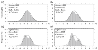
Figure 1 Ensemble-based histograms with 10 240 ensemble members when the Kullback–Leibler (KL) divergence D_KL= (a) 0.010, (b) 0.025, (c) 0.050, and (d) 0.100. Solid lines indicate fitted Gaussian functions. Skewness (Skew) and kurtosis (Kurt) are also shown in the figure.

A non-Gaussian PDF can also be caused by outliers. Although detailed results are shown in Sect. 4, one or several ensemble members are detached from the main cluster; this also results in the large KL divergence D_KL, as well as large skewness and kurtosis, shown in Fig. 2b. We tested two outlier detection methods: the standard deviation-based method (SD method) and the local outlier factor method (LOF method; Breunig et al., 2000). Here, univariate PDFs are considered, so that SD and LOF methods are computed for each variable at each grid point separately.

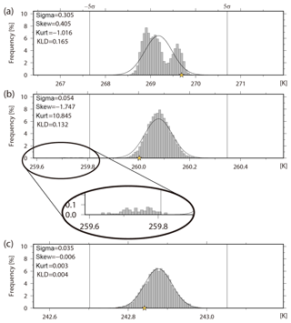
Figure 2 Histograms of background temperature (K) at the fourth model level (∼500 hPa) at (a) grid point A (16.7^∘ S, 90.0^∘ E), (b) grid point B (35.3^∘ N, 146.3^∘ E), and (c) grid point C (35.3^∘ N, 112.5^∘ W). The yellow star shows the truth.

In the SD method, the ensemble members beyond a prescribed threshold in the unit of SD are defined as outliers. If we make 10 240 independent random draws from a Gaussian PDF, statistically 27.6, 0.65, and 0.0059 samples (0.270, 0.00633, and 0.0000573 %) are expected beyond the ±3σ, ±4σ, and ±5σ thresholds, respectively. Hence, using threshold of ±3σ, we would expect to detect 27.6 outliers at every grid point; with the ±4σ threshold, we would expect to detect 1.3 outliers in two grid points (20 480 random draws); with the ±5σ threshold, we would expect to detect 1.18 outliers in 200 grid points (2 048 000 random draws). As outliers appear frequently with ±3σ and ±4σ thresholds, we choose the ±5σ threshold for the SD method in this study.

Unlike the SD method, the LOF method is based on the local density, not on the distance from the sample mean. For a given two-dimensional dataset D, let d(p, o) denote the distance between two objects p∈D and o∈D. For any positive integer k, define k-distance(p) to be the distance between the object p and the kth nearest neighbor. The k-distance neighborhood of p, or simply N_k(p), is defined as the k nearest objects:

$$\begin{array}{}\text{(4)}& N_k\left(p\right)=\mathit{\{}q\in D|q\ne p,d(p,q)\le k\text{-distance}\left(p\right)\mathit{\}}\end{array}$$

The cardinality of N_k(p), or $\left|N_k\right(p\left)\right|$, is greater than or equal to the number of objects (except for the object p itself) within k-distance(p). We define the “reachability distance” of p with respect to the object o as

$$\begin{array}{}\text{(5)}& {\text{reach-dist}}_k(p,o)=\max \mathit{\left\{}k\text{-distance}\right(o),d(p,o\left)\mathit{\right\}}\end{array}$$

That is, if the object p is sufficiently distant from object o, reach-dist_k(p,o) is d(p,o). If they are close enough to each other, reach-dist_k(p,o) is replaced by k-distance(o) instead of d(p,o). Figure 3 shows a schematic diagram of reach-dist_k(p,o) with k=3. N_k(p) includes o₁, o₂, o₃, and o₄, and $\left|N_k\right(p\left)\right|$ is 4. In Fig. 3a, reach-dist_k(p,o₁) is k-distance$\left(o_{\mathrm{1}}\right)=\mathrm{d}(o_{\mathrm{1}},o_{\mathrm{4}})$ because k-distance(o₁) is greater than d(p,o₁). In contrast, in Fig. 3b, reach-dist_k(p,o₁) is d(p,o₁). We further define the “local reachability density” of p, or simply lrd_k(p), as the inverse of the average of reachability distance of p:

$$\begin{array}{}\text{(6)}& {\mathrm{lrd}}_k\left(p\right)={\displaystyle \frac{\left|N_k\left(p\right)\right|}{\sum _{o\in N_k\left(p\right)}{\text{reach-dist}}_k\left(p,o\right)}}.\end{array}$$

Finally, the local outlier factor of p, denoted as LOF_k(p), is defined as

$$\begin{array}{}\text{(7)}& {\mathrm{LOF}}_k\left(p\right)={\displaystyle \frac{\sum _{o\in N_k\left(p\right)}\frac{{\mathrm{lrd}}_k\left(o\right)}{{\mathrm{lrd}}_k\left(p\right)}}{\left|N_k\left(p\right)\right|}}.\end{array}$$

Given a lower local reachability density of p and a higher local reachability density of p's k-nearest neighbors, LOF_k(p) becomes higher. LOF_k(p) or simply LOF is approximately 1 for an object deep within a cluster, and LOF becomes larger around the edge of the cluster due to sparse objects on the far side of the cluster. To summarize, the LOF method focuses on the local densities of objects, and outliers are detected by comparing the local densities. For instance, when k=3 in Fig. 3a, the local densities of the objects p and $o_{\mathrm{1},\mathrm{2},\mathrm{3},\mathrm{4},\mathrm{5}}$ all have similar values because the k-distance(p) is similar to the k-distances$\left(o_{\mathrm{1},\mathrm{2},\mathrm{3},\mathrm{4},\mathrm{5}}\right)$. Therefore, they are not identified as outliers. In contrast, in Fig. 3b the object p has a smaller local density than the other objects $o_{\mathrm{1},\mathrm{2},\mathrm{3},\mathrm{4},\mathrm{5}}$ because k-distance(p) > k-distances($o_{\mathrm{1},\mathrm{2},\mathrm{3},\mathrm{4},\mathrm{5}}$). Therefore, the object p has a larger LOF and is identified as an outlier. An object with a LOF much larger than 1 may be categorized as an outlier, but it is not clear how to determine the threshold for outliers because the threshold also depends on the dataset. The threshold of LOF is chosen to be 8.0 in this study, and Sect. 4 shows the results with different threshold values and discusses why we choose this specific value. k is a control parameter for the LOF method and depends on the dataset, as shown by Breunig et al. (2000), who suggested that choosing a k value from 10 to 20 works well for most of the datasets. If we choose a k value that is too small, some objects deeply inside a cluster have a large LOF, and the LOF method does not work. In fact, using the dataset of KM16, k=10 showed this problem, whereas k=20 did not. Therefore, we chose k=20 in this study. Similar to the SD method, the LOF method is applied to a one-dimensional dataset consisting of 10 240 ensemble members.

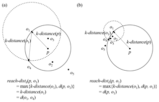
Figure 3 Schematic diagrams of reach-dist_k(p,o) with k=3 for (a) uniformly distributed data and (b) data with an asymmetrical distribution.

The statistics of the KL divergence, and the SD and LOF methods with 10 240 samples are evaluated numerically with 1 million trials of 10 240 random draws from the standard normal distribution by the Box–Muller method (Box and Muller, 1958). The results show that the expected value of KL divergence D_KL is 0.0025, and its standard deviation is 0.00048. As for outlier detections, 5767 and 16 088 trials have at least one outlier for the SD and LOF methods, respectively. Thus, the probabilities to detect at least one outlier at a grid point are 0.58 % for the SD method and 1.6 % for the LOF method. Here, the threshold for the SD method is ±5σ. For the LOF method, we choose k=20 and, as discussed below in Sect. 4, the threshold value LOF is equal to 8.0.

3 Experimental settings

We use the 10 240-member global atmospheric analysis data from an idealized LETKF experiment of KM16. That is, the experiment was performed with the SPEEDY-LETKF system (Miyoshi, 2005) consisting of the SPEEDY model (Molteni, 2003) and the LETKF (Hunt et al., 2007; Miyoshi and Yamane, 2007). The SPEEDY model is an intermediate AGCM based on the primitive equations at T30/L7 resolution, which corresponds to 96×48 grid points in the horizontal and seven levels in the vertical, and has simplified forms of physical parametrization schemes including large-scale condensation, cumulus convection (Tiedtke, 1993), clouds, short- and long-wave radiation, surface fluxes, and vertical diffusion. Due to the very low computational cost, the SPEEDY model has been used in many studies on data assimilation (e.g., Miyoshi, 2005; Greybush et al., 2011; Miyoshi, 2011; Amezcua et al., 2012; Miyoshi and Kondo, 2013; Kondo et al., 2013; MKI14; KM16).

The LETKF applies the ETKF (Bishop et al., 2001) algorithm to the local ensemble Kalman filter (LEKF; Ott et al., 2004). The LETKF can assimilate observations at every grid point independently, which is particularly advantageous in high-performance computation. In fact, Miyoshi and Yamane (2007) showed that the parallelization ratio reached 99.99 % on the Japanese Earth Simulator supercomputer, and KM16 performed 10 240-member SPEEDY-LETKF experiments within 5 min for one execution of LETKF, not including the forecast part on 4608 nodes of the Japanese K supercomputer. The LETKF is computed as follows. Let X (δX) denote an n×m matrix, where the columns are composed of m ensemble members (deviations from the mean of the ensemble) with the system dimension n. The superscripts a and f denote the analysis and forecast, respectively. The analysis ensemble X^a is written as

$$\begin{array}{}\text{(8)}& \begin{array}{rl}{\mathbf{X}}^{\mathrm{a}}={\stackrel{\mathrm{‾}}{\mathbf{x}}}^f\mathbf{1}+\mathit{\delta }{\mathbf{X}}^f& \left[{\stackrel{\mathrm{̃}}{\mathbf{P}}}^{\mathrm{a}}(\mathbf{H}\mathit{\delta }{\mathbf{X}}^f{)}^T{\mathbf{R}}^{-\mathrm{1}}\left({\mathbf{y}}^o-\mathbf{H}{\stackrel{\mathrm{‾}}{\mathbf{x}}}^f\right)\mathbf{1}\right.\\ & \left.+\sqrt{m-\mathrm{1}}{\left({\stackrel{\mathrm{̃}}{\mathbf{P}}}^{\mathrm{a}}\right)}^{\mathrm{1}/\mathrm{2}}\right]\end{array}\end{array}$$

(cf. Eqs. (6) and (7) of Miyoshi and Yamane, 2007). Here, ${\stackrel{\mathrm{‾}}{\mathbf{x}}}^f$, y^o, H, and R denote the background ensemble mean, observations, linear observation operator, and observation error covariance matrix, respectively. 1 is an m-dimensional row vector with all elements being 1. The m×m analysis error covariance matrix ${\stackrel{\mathrm{̃}}{\mathbf{P}}}^{\mathrm{a}}$ in the ensemble space is given as

$$\begin{array}{}\text{(9)}& {\stackrel{\mathrm{̃}}{\mathbf{P}}}^{\mathrm{a}}={\left[\left(m-\mathrm{1}\right)\mathbf{I}/\mathit{\rho }+\left(\mathbf{H}\mathit{\delta }{\mathbf{X}}^f{)}^T{\mathbf{R}}^{-\mathrm{1}}\right(\mathbf{H}\mathit{\delta }{\mathbf{X}}^f)\right]}^{-\mathrm{1}}={\mathbf{UD}}^{-\mathrm{1}}{\mathbf{U}}^T\end{array}$$

(cf. Eqs. (3) and (9) of Miyoshi and Yamane, 2007). Here, ρ denotes the covariance inflation factor. As ${\stackrel{\mathrm{̃}}{\mathbf{P}}}^{\mathrm{a}}$ is real symmetric, U is composed of the orthonormal eigenvectors, such that UU^T=I. The diagonal matrix D is composed of the nonnegative eigenvalues.

KM16 performed a perfect-model twin experiment for 60 d from 00:00 UTC on 1 January in the second year of the nature run, which was initiated at 00:00 UTC on 1 January from the standard atmosphere at rest (zero wind). The first year of the nature run was discarded as spin-up. To resolve detailed PDF structures, the ensemble size was fixed to 10 240. No localization was applied, yielding the best analysis accuracy as shown by KM16, who compared five 10 240-member experiments with different choices of localization: step functions with 2000, 4000, and 7303 km localization radii, a Gaussian function with a 7303 km localization radius, and no localization. The observations for horizontal wind components (U, V), temperature (T), specific humidity (Q), and surface pressure (P_s) were simulated by adding observational errors to the nature run every 6 h at radiosonde-like locations (see Fig. 8, crosses) for all seven vertical levels, but the observations of specific humidity were simulated from the bottom to the fourth model level (about 500 hPa). The observational errors were generated from independent Gaussian random numbers, and the observational error standard deviations were fixed at 1.0 m s⁻¹, 1.0 K, 0.1 g kg⁻¹, and 1.0 hPa for U∕V, T, Q, and P_s, respectively.

The non-Gaussian measures, skewness ${\mathit{\beta }}_{\mathrm{1}}^{\mathrm{1}/\mathrm{2}}$, kurtosis β₂, and KL divergence D_KL, are calculated at each grid point for each variable. Outliers are diagnosed similarly at each grid point for each variable with the SD method and LOF method.

4 Results

Figure 4 shows the spatial distributions of the analysis absolute error, ensemble spread, background skewness ${\mathit{\beta }}_{\mathrm{1}}^{\mathrm{1}/\mathrm{2}}$, kurtosis β₂, and KL divergence D_KL for temperature at the fourth model level (∼500 hPa) at 06:00 UTC on 22 February. When the analysis absolute error is large, the background non-Gaussian measures also tend to be large, especially in the tropics. The peaks for skewness ${\mathit{\beta }}_{\mathrm{1}}^{\mathrm{1}/\mathrm{2}}$, kurtosis β₂, and KL divergence D_KL tend to coincide. Although grid point A (16.7^∘ S, 90.0^∘ E) has a large KL divergence D_KL with large analysis absolute error, at grid point B (35.3^∘ N, 146.3^∘ E) with a large KL divergence D_KL the analysis absolute error is small (< 0.08 K). This result shows that the large analysis error is not always associated with the strong non-Gaussianity at a specific time. The PDFs at grid points A and B are shown in Fig. 2a and b, respectively. The histogram at grid point A is clearly a multimodal PDF with KL divergence D_KL > 0.01, and the right mode captures the truth (yellow star). At grid point B, although the PDF seems to be closer to Gaussian, skewness ${\mathit{\beta }}_{\mathrm{1}}^{\mathrm{1}/\mathrm{2}}$ and kurtosis β₂ are much larger than those at grid point A. In fact, the PDF does not fit to the Gaussian function calculated by the ensemble mean and standard deviation. Zooming in on the left side of Fig. 2b shows a small cluster composed of 76 members detached from the main cluster; 74 members of the small cluster exceed −5σ and are categorized as outliers in the SD method. This small cluster causes the standard deviation to become large and results in the Gaussian function having a longer tail than the histogram. The small cluster should not be considered as consisting of outliers because it may have some physical significance. Scatter diagrams of LOF versus distance from the ensemble mean for all ensemble members at grid points A and B are shown in Fig. 5a and b, respectively. At grid point A, the LOF is not that large, even at the edge of the cluster (< 4), and the multimodal PDF does not influence the LOF. In addition, all members are within ±3σ. Therefore, there are no clear outliers at grid point A. At grid point B, although most of the small cluster exceeds −5σ, the maximum LOF in the small cluster is still smaller than 3. This indicates that all members of the small cluster should not be outliers in the LOF method. As an outlier case, we note the grid point C (35.3^∘ N, 112.5^∘ W) in Fig. 4. The PDF at the grid point C fits the Gaussian function well, and the non-Gaussian measures are quite small (Fig. 2c). A member on the left edge of the scatter diagram in Fig. 5c has the largest LOF > 8.0, but the member is within ±3σ. As mentioned in Sect. 2, the threshold of the LOF for outliers depends on the dataset. Figure 6 shows the number of outliers for thresholds of 5.0, 8.0, and 11.0 at 06:00 UTC on 22 February. There are too many outliers with a threshold of 5.0; however, the number of outliers decreases markedly with thresholds of 8.0 or 11.0. Based on these results, and as already mentioned in Sect. 2, we adopt a LOF of 8.0 as a threshold for outliers.

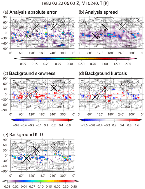
Figure 4 Spatial distributions of (a) analysis absolute error, (b) analysis ensemble spread, (c) background skewness, (d) background kurtosis, and (e) background KL divergence for temperature at the fourth model level (∼500 hPa) at 06:00 UTC on 22 February. Contours indicate geopotential height of the ensemble mean at the 500 hPa level.

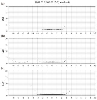
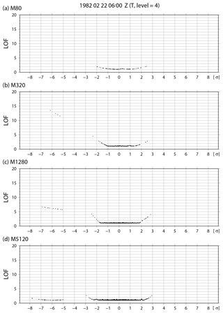
Figure 5 Scatter diagrams of the local outlier factor (LOF) method versus distance from the ensemble mean for all ensemble members for background temperature at the fourth model level (∼500 hPa) at (a) grid point A (16.7^∘ S, 90.0^∘ E), (b) grid point B (35.3^∘ N, 146.3^∘ E), and (c) grid point C (35.3^∘ N, 112.5^∘ W).

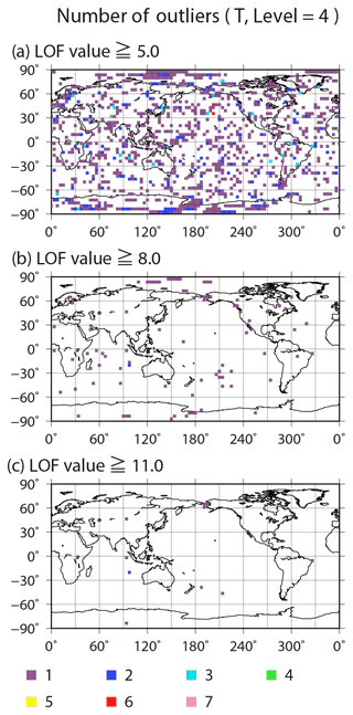
Figure 6 Spatial distributions of the number of outliers for background temperature at the fourth model level (∼500 hPa) at 06:00 UTC on 22 February for LOF thresholds of (a) 5.0, (b) 8.0, and (c) 11.0.

Figure 7 shows the spatial distributions of the time-mean analysis RMSE, the ensemble spread, the background absolute skewness ${\mathit{\beta }}_{\mathrm{1}}^{\mathrm{1}/\mathrm{2}}$, the absolute kurtosis β₂, and the KL divergence D_KL. As mentioned in KM16, the time-mean ensemble spread corresponds well to the RMSE, which is larger in the tropics. The pattern correlation between the RMSE and ensemble spread is 0.97. Moreover, the distributions of non-Gaussian measures are similar to each other and also correspond well to the RMSE and ensemble spread. The RMSE and non-Gaussian measures differ in that the non-Gaussianity is large in storm tracks, such as the North Pacific Ocean and the North Atlantic Ocean. This may be because the LETKF inhibits growing errors well in storm tracks regardless of the strong non-Gaussianity. To investigate the non-Gaussianity in more detail, Figs. 8 and 9 show the frequencies of non-Gaussian PDF with high KL divergence D_KL > 0.01 and the frequencies identifying at least one outlier with high LOF > 8.0 on a 10 240-member ensemble, respectively. The frequency of non-Gaussian PDF is defined as the ratio of non-Gaussianity appearance at every grid point during the 36 d period from 00:00 UTC on 25 January to 18:00 UTC on 1 March. The spatial distribution of the frequency of non-Gaussianity for temperature is similar to that of the time-mean RMSE and D_KL (Figs. 7a, e, 8b), and the pattern correlation between the spatial distribution of the mean RMSE and D_KL is 0.68. We find a high frequency of non-Gaussian PDFs in the tropics and storm track regions for temperature, specific humidity, and surface pressure, although non-Gaussian PDFs seldom appear in the densely observed regions. In the tropics, the frequency reaches up to 90 %, and in South America the frequency reaches the highest value of over 95 %, i.e., the non-Gaussian PDF appears for 34 d out of 36 d. In contrast, the non-Gaussian PDF for zonal wind hardly appears (Fig. 8a), and the intensity of the non-Gaussianity, as evaluated by other measures, is also weak (not shown). Conversely, the outliers appear almost randomly and do not clearly depend on the region for any of the variables (Fig. 9); most outliers also disappear within only one or a few analysis steps. Moreover, there are no correlations between the frequency of outliers and the analysis RMSE.

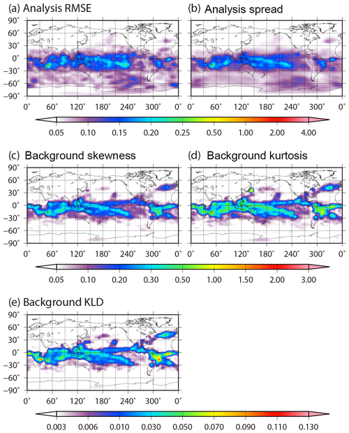
Figure 7 Spatial distributions of the time-mean (a) analysis RMSE, (b) analysis ensemble spread, (c) background absolute skewness, (d) background absolute kurtosis, and (e) background KL divergence for temperature at the fourth model level (∼500 hPa) from 00:00 UTC on 25 January to 18:00 UTC on 1 March.

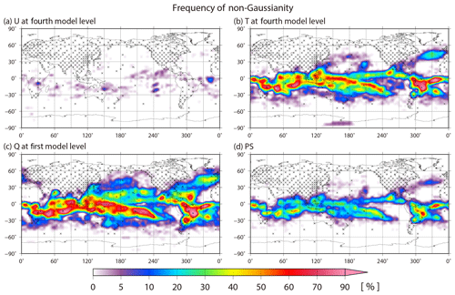
Figure 8 Spatial distributions of the frequency of the non-Gaussian PDF with high KL divergence D_KL > 0.01 for (a) zonal wind at the fourth model level, (b) temperature at the fourth model level, (c) specific humidity at the lowest model level, and (d) surface pressure. The frequency is defined as a ratio of high KL divergence D_KL appearance from 00:00 UTC on 25 January to 18:00 UTC on 1 March. The crosses indicate the radiosonde-like locations.

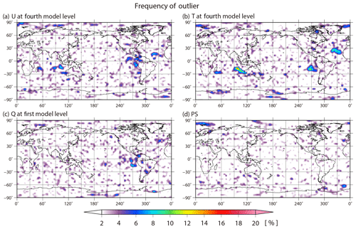
Figure 9 Similar to Fig. 8, but showing the frequency of identifying at least one outlier with high a LOF > 8.0 on a 10 240-member ensemble.

To investigate how the non-Gaussian PDF is generated, we plot the forecast and analysis update processes at 1.9^∘ N, 168.7^∘ E for 256 members chosen randomly from 10 240 members from the analysis at 00:00 UTC on 9 February (157th analysis cycle) to the forecast at 00:00 UTC on 10 February (161st analysis cycle, Fig. 10a). That is, Fig. 10a shows the life cycle of the non-Gaussian PDF. As the y axis, we introduce the convective instability dθ_e, which is defined as a difference between equivalent potential temperature θ_e at the fourth model level (∼500 hPa) and θ_e at the second model level (∼850 hPa). Negative (positive) dθ_e indicates a convectively unstable (stable) atmosphere. The non-Gaussian PDF appears in the background at the 159th cycle (12:00 UTC, 9 February), and the model forecast increases the KL divergence D_KL for dθ_e up to 0.154 with a bimodal PDF of clusters A and B. We find many lines crossing in the forecast step from the analyses at the 158th cycle to the background at the 159th cycle. Thus, many of the upper side cluster A at the 159th cycle come from the lower side analyses in the previous 158th cycle, generally reducing the instability (increasing values of dθ_e) in the forecast step, and vice versa for the lower side cluster B. In the background temperature at the fourth model level, the KL divergence D_KL also increases from 0.003 to 0.299 for 6 h (Fig. 10b, c). Finally, the non-Gaussian PDF almost disappears at the 161st cycle (00:00 UTC, 10 February). Figure 11 shows a scatter diagram of 06:00 UTC versus 12:00 UTC on 9 February for background temperature in the fourth model level for each member at 1.9^∘ N, 168.7^∘ E, and also shows histograms corresponding to the scatter diagrams. The PDF at 06:00 UTC is almost Gaussian. However, at 12:00 UTC, the bimodal structure with KL divergence D_KL=0.299 appears. The dot colors show $\mathrm{d}{\mathit{\theta }}_{\mathrm{e}}^{\prime }$ evaluated from 06:00 to 12:00 UTC on 9 February, namely, $\mathrm{d}{\mathit{\theta }}_{\mathrm{e}}^{\prime }=\left(\mathrm{d}{\mathit{\theta }}_{\mathrm{e}\mathrm{12}:\mathrm{00}\mathrm{UTC}}-\mathrm{d}{\mathit{\theta }}_{\mathrm{e}\mathrm{06}:\mathrm{00}\mathrm{UTC}}\right)-\left(\mathrm{d}{\stackrel{\mathrm{‾}}{\mathit{\theta }}}_{\mathrm{e}\mathrm{12}:\mathrm{00}\mathrm{UTC}}-\mathrm{d}{\stackrel{\mathrm{‾}}{\mathit{\theta }}}_{\mathrm{e}\mathrm{06}:\mathrm{00}\mathrm{UTC}}\right)$, where ${\stackrel{\mathrm{‾}}{\mathit{\theta }}}_{\mathrm{e}}$ indicates the equivalent potential temperature calculated from the ensemble mean. That is, a red (blue) dot shows more stability (instability) than the ensemble mean. The red and blue dots are clearly divided into the right and left side modes, respectively. Most members with mitigated (enhanced) instability move to the right (left) side mode. The members with larger (smaller) temperature values at 12:00 UTC correspond to larger (smaller) values of stability as shown by the warmer (colder) color. In addition, both right and left modes correspond to the opposite side modes in the specific humidity, respectively (not shown). That is, the members with higher (lower) temperature have lower (higher) humidity than the ensemble mean. The instability is driven by precipitation. Figure 12 is similar to Fig. 11, but for precipitation. The 10 240 members are clearly divided into three clusters at 12:00 UTC by the instability. The three clusters indicate the number of times cumulus parameterization is triggered. Most members in the right (left) cluster are red (blue) and show mitigation (enhancement) of the instability. Figure 13 is also similar to Fig. 11, but for zonal wind at the fourth model level. In agreement with what has been seen on Fig. 8a, the non-Gaussianity of zonal wind is weak, and the bimodal structure appearing in temperature and humidity seldom affects the PDF of zonal wind. We found no relationship between the atmospheric instability and zonal wind. Therefore, the genesis of non-Gaussian PDF in the tropics is deeply related to precipitation process, which is driven by convective instability through cumulus parameterization in the SPEEDY model. As a result, the precipitation process mitigates the instability, with rising temperature and decreasing humidity. Similar results are generally obtained at other grid points with non-Gaussian PDF.

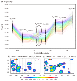
Figure 10 Life cycle of non-Gaussianity at 1.9^∘ N, 168.7^∘ E. (a) Trajectories of 256 randomly chosen members from 10 240 members for dθ_e (see text for definition) from an analysis at the 157th analysis cycle (00:00 UTC, 9 February) to forecast the 161st analysis cycle (00:00 UTC, 10 February). The colors show the order of dθ_e for every analysis. D_KL shows KL divergence for dθ_e, and the superscripts a and f indicate analysis and forecast, respectively. (b, c) Spatial distributions of KL divergence for background temperature at the fourth model level (∼500 hPa) at the 158th analysis cycle (06:00 UTC, 9 February) and the 159th analysis cycle (12:00 UTC, 9 February), respectively. The cross shows the location of the point considered in panel (a).

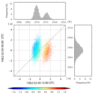
Figure 11 Scatter diagram of 06:00 UTC versus 12:00 UTC on 9 February for the background temperature at the fourth model level (∼500 hPa) at 1.9^∘ N, 168.7^∘ E. The colors show $\mathrm{d}{\mathit{\theta }}_{\mathrm{e}}^{\prime }=\left(\mathrm{d}{\mathit{\theta }}_{\mathrm{e}\mathrm{12}:\mathrm{00}\mathrm{UTC}}-\mathrm{d}{\mathit{\theta }}_{\mathrm{e}\mathrm{06}:\mathrm{00}\mathrm{UTC}}\right)-\left(\mathrm{d}{\stackrel{\mathrm{‾}}{\mathit{\theta }}}_{\mathrm{e}\mathrm{12}:\mathrm{00}\mathrm{UTC}}-\mathrm{d}{\stackrel{\mathrm{‾}}{\mathit{\theta }}}_{\mathrm{e}\mathrm{06}:\mathrm{00}\mathrm{UTC}}\right)$ The histograms in the right and upper panels show the background temperature at the same grid point.

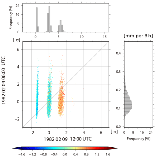
Figure 12 Similar to Fig. 11, but for 06:00 UTC versus 12:00 UTC on 9 February for background precipitation.

In the extratropics, non-Gaussian PDF is generated differently. To investigate the genesis of non-Gaussian PDF in the extratropics, we focus on a case around an extratropical cyclone over the Atlantic Ocean. A non-Gaussian PDF appears at 06:00 UTC on 15 February at 42.7^∘ N, 48.8^∘ W, and the KL divergence D_KL of background temperature increases from 0.003 to 0.460 (Fig. 14, crosses). Figure 15 is similar to Fig. 11, but for background specific humidity at the second model level (∼850  hPa) versus precipitation at 42.7^∘ N, 48.8^∘ W at 00:06 UTC on 15 February. Trimodal PDFs appear in both specific humidity and precipitation. The three modes of specific humidity are clearly separated by the color, i.e., instability $\mathrm{d}{\mathit{\theta }}_{\mathrm{e}}^{\prime }$: modes with larger humidity have colder colors (smaller $\mathrm{d}{\mathit{\theta }}_{\mathrm{e}}^{\prime }$ corresponding to more instability). However, the three modes of precipitation show no clear dependence on $\mathrm{d}{\mathit{\theta }}_{\mathrm{e}}^{\prime }$. Therefore, the trimodal PDF of specific humidity would not be driven by the cumulus parameterization. Next, the relationship between background specific humidity and meridional wind at the second model level (∼850 hPa) is shown in Fig. 16. The members in the left mode have lower specific humidity with relatively stronger northerly wind. If we look at the fourth model level (∼500 hPa) for these members with lower humidity, they have relatively weaker northerly wind and warm temperature (not shown). Thus, instabilities are mitigated by the northerly advection of dry air in the lower troposphere and by warm temperature in the mid troposphere. In this case study, the non-Gaussianity genesis in the extratropics is associated with the advections. This is only an example, and the non-Gaussianity genesis in the extratropics is generally more complicated and would be affected not only by vertical stratification but also by larger-scale atmospheric phenomena such as extratropical cyclones and advections. Here, we do not go into details for different cases of non-Gaussianity genesis, but instead, this is further discussed in Sect. 5.

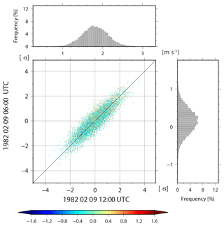
Figure 13 Similar to Fig. 11, but for 06:00 UTC versus 12:00 UTC on 9 February for background zonal wind at the fourth model level (∼500 hPa).

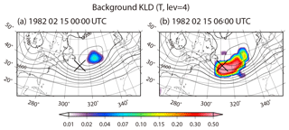
Figure 14 Spatial distributions of the KL divergence for background temperature at the fourth model level (∼500 hPa) (a) at 00:00 UTC on 15 February and (b) at 06:00 UTC on 15 February. Contours show geopotential height of the ensemble mean at the 500 hPa level.

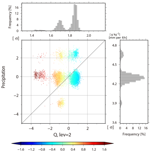
Figure 15 Scatter diagram of background specific humidity at the second model level (∼850 hPa) versus background precipitation at 42.7^∘ N, 48.8^∘ W (311.3^∘ E) at 06:00 UTC on 15 February. The colors show $\mathrm{d}{\mathit{\theta }}_{\mathrm{e}}^{\prime }=\left(\mathrm{d}{\mathit{\theta }}_{\mathrm{e}\mathrm{06}:\mathrm{00}\mathrm{UTC}}-\mathrm{d}{\mathit{\theta }}_{\mathrm{e}\mathrm{00}:\mathrm{00}\mathrm{UTC}}\right)-\left(\mathrm{d}{\stackrel{\mathrm{‾}}{\mathit{\theta }}}_{\mathrm{e}\mathrm{06}:\mathrm{00}\mathrm{UTC}}-\mathrm{d}{\stackrel{\mathrm{‾}}{\mathit{\theta }}}_{\mathrm{e}\mathrm{00}:\mathrm{00}\mathrm{UTC}}\right)$ The histograms in the right and upper panels show background precipitation and temperature at the same grid point, respectively.

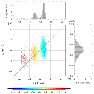
Figure 16 Similar to Fig. 14, but for background specific humidity versus meridional wind background at the second level (∼850 hPa).

The non-Gaussian measures are sensitive to the ensemble size due to sampling errors. Figure 17 shows the spatial distributions of the skewness ${\mathit{\beta }}_{\mathrm{1}}^{\mathrm{1}/\mathrm{2}}$, kurtosis β₂, and KL divergence D_KL for temperature at the fourth model level (∼500 hPa) at 06:00 UTC on 22 February with 80, 320, and 1280 subsamples from 10 240 members, respectively. Skewness ${\mathit{\beta }}_{\mathrm{1}}^{\mathrm{1}/\mathrm{2}}$, kurtosis β₂, and KL divergence D_KL with 80 members contain high levels of contaminating errors originating from sampling errors, and the non-Gaussian measures are difficult to distinguish from the contaminating errors. When increasing the ensemble size up to 1280, the sampling errors become smaller by gradation. With 1280 members, the sampling errors are essentially removed, and the distributions are comparable to those with 10 240 members (see Fig. 4). Therefore, a sample size of about 1000 members is necessary to represent a non-Gaussian PDF. The outliers are also depend on the sample size. Figure 18 shows LOF with 80, 320, 1280, and 5120 subsamples from 10 240 members for temperature at the fourth model level at grid point B (35.3^∘ N, 146.3^∘ E), as in Fig. 5b. With 80 members, there are no outliers as the LOF of each member is much smaller than the outlier threshold of 8.0. When the ensemble size is 320, four members with a high LOF > 8.0 are identified as outliers. With the ensemble sizes of 1280 and 5120, 13 and 41 members construct a small cluster, respectively, but they are not outliers with the threshold of LOF = 8.0. When increasing the ensemble size up to 10 240, the LOFs of the small cluster and main cluster show almost the same value (Fig. 5b).

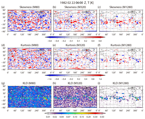
Figure 17 Spatial distributions of (a–c) skewness, (d–f) kurtosis, and (g–i) KL divergence for temperature at the fourth model level (∼500 hPa) at 06:00 UTC on 22 February. The left, center, and right columns show 80, 320, and 1280 subsamples from 10 240 members, respectively.

Figure 18 Similar to Fig. 5b, but for the ensemble sizes (a) 80, (b) 320, (c) 1280, and (d) 5120.

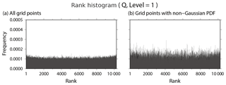
Figure 19 Rank histograms verified against truth for background specific humidity at the lowest model level (∼925 hPa) at (a) all grid points and (b) the grid points with non-Gaussian PDF from 00:00 UTC on 25 January to 18:00 UTC on 1 March.

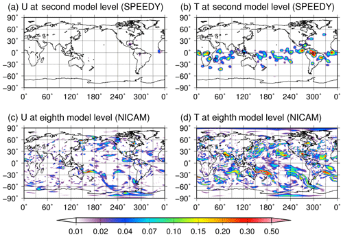
Figure 20 Spatial distributions of background KL divergence for the SPEEDY and NICAM models. Upper panels show (a) zonal wind and (b) temperature at the second model level (∼850 hPa) for the SPEEDY model at 00:00 UTC on 1 March. Bottom panels show (c) zonal wind and (d) temperature at the eighth model level (∼850 hPa) for NICAM at 00:00 UTC on 8 November 2011.

We saw good agreement between the RMSE and ensemble spread (Fig. 7a, b), but it is useful to further evaluate the 10 240-member ensemble using ranked probability scores. The rank histogram (Hamill and Collucci, 1997; Talagrand et al., 1999; Anderson, 1996; Hamill, 2001) evaluates the reliability of ensemble statistically. Figure 19 shows almost flat rank histograms at all grid points and the grid points with non-Gaussian PDF. The truth is known in this study and used as a verifying analysis. The flat rank histograms correspond to healthy background ensemble distributions. The continuous ranked probability score (CRPS, Hersbach, 2000) is another method to evaluate ensemble distributions, decomposed into reliability, resolution and uncertainty as

$$\begin{array}{}\text{(10)}& \mathrm{CRPS}=\mathrm{Reli}-\mathrm{Resol}+U.\end{array}$$

Here, the reliability (Reli) becomes zero under the perfectly reliable system. The resolution (Resol) indicates the degree to which the ensemble distinguishes situations with different frequencies of occurrence, and is associated with the accuracy or sharpness. The uncertainty (U) measures the climatological variability. The reliability, resolution and uncertainty are given on the prescribed area as

$$\begin{array}{}\text{(11)}& {\displaystyle }\begin{array}{rl}\mathrm{Reli}& =\sum _{i=\mathrm{0}}^N{\stackrel{\mathrm{‾}}{g}}_i{\left({\stackrel{\mathrm{‾}}{o}}_i-p_i\right)}^{\mathrm{2}}\\ p_i& ={\displaystyle \frac{i}{N}}\end{array}\text{(12)}& {\displaystyle }U-\mathrm{Resol}=\sum _{i=\mathrm{0}}^N{\stackrel{\mathrm{‾}}{g}}_i{\stackrel{\mathrm{‾}}{o}}_i\left(\mathrm{1}-{\stackrel{\mathrm{‾}}{o}}_i\right)\text{(13)}& {\displaystyle }U=\sum _{k,l<k}{w}_k{w}_l\left|y^k-y^l\right|\end{array}$$

(cf. Eqs. (36), (37) and (19) in Hersbach, 2000, respectively). Here, ${\stackrel{\mathrm{‾}}{g}}_i$ is the area-weighted average width of the bin i between consecutive ensemble members x_i and x_i+1, and ${\stackrel{\mathrm{‾}}{o}}_i$ is the area-weighted average frequency that the verifying analysis is less than $\left(x_{i+\mathrm{1}}+x_i\right)/\mathrm{2}$. N denotes an ensemble size. In this study, y^k and y^l indicate the anomalies between the background ensemble mean and monthly climatology computed from a 30-year nature run at the grid points k and l, respectively. The weights w_k, w_l are proportional to the cosine of latitude. Table 1 shows that the reliability is closer to zero and that the resolution is much higher at all grid points than at the grid points with non-Gaussian PDF. Therefore, the non-Gaussian PDF has a negative impact on updating the state variables for the LETKF. The smaller uncertainty at the grid points with non-Gaussian PDF reflects generally smaller variations in the tropics where the non-Gaussian PDFs frequently appear. Similar results are obtained for the other variables.

Table 1 CRPS and its three components (reliability, resolution, and uncertainty) for background specific humidity at the lowest model level (∼925 hPa) from 00:00 UTC on 25 January to 18:00 UTC on 1 March.

5 Summary and discussions

Kalman filters provide the minimum variance linear estimator, which coincides with the maximum likelihood estimator if the PDFs are Gaussian. This study investigated the non-Gaussian PDF and its behavior using the SPEEDY-LETKF system with 10 240 members. Non-Gaussian PDFs appear frequently in the areas where the RMSE and ensemble spread are larger. Moreover, an ensemble size of about 1000 is necessary to identify the possible non-Gaussianity of PDFs, which may be difficult to detect in the presence of sampling error.

The non-Gaussian PDF frequently appears in the tropics and the storm track regions over the Pacific and Atlantic oceans, particularly for temperature and specific humidity, but not for winds. With the SPEEDY model, the genesis of non-Gaussian PDF in the tropics is mainly associated with the convective instability. These results suggest that the non-Gaussianity is mainly caused by precipitation processes such those associated with cumulus convection, but much less by dynamic processes. Generally, the atmosphere in the tropics tends to become unstable, and the convective instability is mitigated by vertical convection with precipitation. In the SPEEDY model, a simplified mass-flux scheme developed by Tiedtke (1993) is applied. Convection occurs when either the specific or relative humidity exceeds a prescribed threshold (Molteni, 2003). The members that hit the threshold have precipitation, and this process mitigates their own convective instability resulting in a temperature rise and humidity decrease. In contrast, the members with no or little precipitation enhance or cannot mitigate their own convective instability. Therefore, convective instability is a key to non-Gaussianity genesis in the tropics in the SPEEDY model.

In the extratropics, non-Gaussianity is generally weak and seldom appears except in the storm track regions, where the genesis of the non-Gaussian PDF is also associated with instabilities, but with different processes from the tropics. This study focused on a case near the extratropical cyclone in the North Atlantic, and the results showed that the instability was associated with the horizontal advections. The members with reduced instabilities had lower humidity in the lower troposphere and higher temperature in the mid troposphere by meridional advections. In contrast, the members with higher humidity in the lower troposphere and lower temperature in the mid troposphere enhanced their instability. Moreover, the precipitation process through the cumulus parameterization did not explain the non-Gaussian PDF. Precipitation associated with extratropical cyclones is usually caused by synoptic-scale baroclinic instabilities and does not mitigate the local instability completely.

As mentioned in Sect. 4, generalizing the process of non-Gaussianity genesis in the extratropics is not simple. The non-Gaussianity genesis is generally associated with instability from various processes such as the convection, advection, and larger-scale atmospheric phenomena, so that it is very difficult to find general mechanisms of the non-Gaussianity genesis in the extratropics even for the simple SPEEDY model. Furthermore, if we use more realistic models with complex physics schemes, the process of non-Gaussianity genesis would be much more diverse and complicated. This is partly why we did not go into details to investigate different cases of non-Gaussianity genesis with the SPEEDY model.

The non-Gaussianity is less frequent in the wind components not only on the timescale of 1 month but also for the snapshot, although the dynamic process of the atmosphere is a nonlinear system. Moreover, the non-Gaussian PDFs of temperature and specific humidity seldom affect the PDFs of the wind components. We hypothesize that the model complexity may be a reason for this. The SPEEDY model could not resolve some local interactions between wind components and other variables due to its coarse resolution and simplified processes. With more realistic models, physical processes are much more complex, and the local interactions can also be represented. Indeed, we obtained widely distributed non-Gaussianity with a 10 240-member NICAM-LETKF system with a 112 km horizontal resolution assimilating real observations from the National Centers for Environmental Prediction (NCEP) known as PREPBUFR from 00:00 UTC on 1 November to 00:00 UTC on 8 November (Miyoshi et al., 2015). Figure 20 shows the spatial distributions of background KL divergence of zonal wind and temperature at the second model level (∼850 hPa) for SPEEDY at 00:00 UTC on 1 March and zonal wind and temperature at the eighth model level (∼850 hPa) for the NICAM at 00:00 UTC on 8 November 2011. With NICAM, the non-Gaussianity appears globally not only in the temperature field but also in the zonal wind, although we should account for the model errors of NICAM. This result implies that the NICAM has various sources of non-Gaussianity such as smaller-scale physical and dynamical processes with various interactions among different model variables, and suggests the limitation of this study using the SPEEDY model. In a realistic situation, we would presumably have more frequent occurrence of non-Gaussianity.

The outliers appear almost randomly regardless of locations, levels, and variables, and the lifetime is about a few analysis steps. When the outliers appear, the number of outliers is basically one per grid point, but sometimes the number is more than one. Anderson (2010) also reported similar results using a low-order dry atmospheric model. These results seem not to be consistent with Amezcua et al. (2012), who reported that just one outlier appeared with the ensemble square root filters in low-dimensional models and that the outlier did not rejoin the cluster easily. These properties of their outlier and our outliers in the SPEEDY model are somewhat different. In the low-dimensional models, a certain ensemble member tends to become an outlier at all grid points and all variables. In contrast, the outliers in the SPEEDY model appear at just some grid points but not all grid points and do not appear in all variables simultaneously. In addition, the negative influence of outliers on the analysis accuracy may be quite small in high-dimensional models due to the randomness and short longevity of outliers. In fact, the results showed no clear correspondence between the outlier frequency and analysis accuracy. These are the results from the simple SPEEDY model. How the outliers behave with a more realistic model and real observations remains the subject of future research.

As measures of non-Gaussianity, skewness, kurtosis, and KL divergence for the non-Gaussianity, and the SD and LOF methods for outliers, are introduced and compared with each other. The KL divergence is a more suitable measure because it measures the direct difference between the ensemble-based histogram and the fitted Gaussian function. The LOF method is better than the SD method because it can detect the outliers depending on the density of objects. Although it is easy to detect the outliers using the SD method, misdetection of outliers is possible because this method categorizes a small cluster far from the main cluster into outliers. The small cluster may be generated via physical processes and have physical significance; therefore, such cases should not be treated as outliers. The measures of non-Gaussianity are evaluated in the univariate field in this study. An extension to multivariate fields with multivariate analysis remains a subject for future research.

Non-Gaussian measures tend to be more sensitive to the sampling error due to the limited ensemble size (see Figs. 17, 18). When the ensemble size is small, it is difficult to determine whether a split member is a real outlier or a sample from a small cluster. Amezcua et al. (2012) discussed the outliers by skewness using the 20-member SPEEDY-LETKF and reported that the skewness is clearly large in the tropics and the Southern Hemisphere for the temperature and humidity fields. These results were not consistent with those of the present study because the outliers appear randomly. However, this inconsistency may have been due to the small ensemble size. The large skewness of Amezcua et al. (2012) could possibly indicate the non-Gaussianity rather than the outliers with a large ensemble size. Having a sufficient ensemble size, suggested to be about 1000 according to this study, would be essential when discussing about non-Gaussianity and outliers.