A Bayesian approach to multivariate adaptive localization in ensemble-based data assimilation with time-dependent extensions

Ever since its inception, the ensemble Kalman filter (EnKF) has elicited many heuristic approaches that sought to improve it. One such method is covariance localization, which alleviates spurious correlations due to finite ensemble sizes by using relevant spatial correlation information. Adaptive localization techniques account for how correlations change in time and space, in order to obtain improved covariance estimates. This work develops a Bayesian approach to adaptive Schur-product localization for the deterministic ensemble Kalman filter (DEnKF) and extends it to support multiple radii of influence. We test the proposed adaptive localization using the toy Lorenz'96 problem and a more realistic 1.5-layer quasi-geostrophic model. Results with the toy problem show that the multivariate approach informs us that strongly observed variables can tolerate larger localization radii. The univariate approach leads to markedly improved filter performance for the realistic geophysical model, with a reduction in error by as much as 33 %.

1 Introduction

Data assimilation (Asch et al., 2016; Law et al., 2015; Evensen, 2009; Reich and Cotter, 2015) fuses information from the model forecast states (Eq. 1) and observations (Eq. 3) in order to obtain an improved estimation of the truth at any given point in time. Data assimilation approaches include the ensemble Kalman filters (EnKFs) (Evensen, 1994, 2009; Constantinescu et al., 2007b) that rely on Gaussian assumptions, particle filters for non-Gaussian distributions (Van Leeuwen et al., 2015; Attia et al., 2017; Attia and Sandu, 2015), and variational approaches, rooted in control theory (Le Dimet and Talagrand, 1986; Sandu et al., 2005; Carmichael et al., 2008).

EnKF is an important family of data assimilation techniques that propagate both the mean and covariance of the state uncertainty through the model using a Monte Carlo approach. While large dynamical systems of interest have a large number of modes along which errors can grow, the number of ensemble members used to characterize uncertainty remains relatively small due to computational costs. As a result, inaccurate correlation estimates obtained through Monte Carlo sampling can profoundly affect the filter results. Techniques such as covariance localization and inflation have been developed to alleviate these problems (Petrie and Dance, 2010).

Localization techniques take advantage of the fundamental property of geophysical systems that correlations between variables decrease with spatial distance (Kalnay, 2003; Asch et al., 2016). This prior knowledge is used to scale ensemble-estimated covariances between distant variables so as to reduce inaccurate, spurious correlations. The prototypical approach to localization is a Schur-product-based tapering of the covariance matrix (Bickel and Levina, 2008); theoretical results ensure that the covariance matrices estimated using small ensembles sampled from a multivariate normal probability distribution, upon tapering, approach quickly the true covariance matrix. A formal theory of localization (Flowerdew, 2015) has been attempted, though a true multivariate theory is still out of our grasp. Practical implementations of localization rely on restricting the information flow, either in state space or in observation space, to take place within a given “radius of influence” (Hunt et al., 2007). Some variants of EnKF like the maximum likelihood ensemble filter (MLEF) (Zupanski, 2005) reduce the need for localization, while others use localization in order to efficiently parallelize the analysis cycles in space (Nino-Ruiz et al., 2015).

The performance of the EnKF algorithms critically depends on the correct choice of localization radii (also known as the decorrelation distances), since values that are too large fail to correct for spurious correlations, while values that are too small throw away important correlation information. However, the physical values of the spatial decorrelation scales are not known a priori, and they change with the temporal and spatial location. At the very least the decorrelation scales depend on the current atmospheric flow. In atmospheric chemistry systems, because of the drastic difference in reactivity, each chemical species has its own individual localization radius (Constantinescu et al., 2007a). Multi-scale schemes (Buehner and Shlyaeva, 2015) for localization are an immediate necessity. Clearly, the widely used approach of estimating decorrelation distances from historical ensembles of simulations and then using a constant averaged value throughout the space and time domain leads to a suboptimal performance of ensemble Kalman filters.

Adaptive localization schemes seek to estimate decorrelation distances from the data, so as to optimize the filter performance according to some criteria. One approach to adaptive localization utilizes an ensemble of ensembles to detect and mitigate spurious correlations (Anderson, 2007). Relying purely on model dynamics and foregoing reliance on spatial properties of the model, the method is very effective for small-scale systems, but its applicability to large-scale geophysical problems is unclear. There is, however, evidence that optimal localization depends more on ensemble size and observation properties than on model dynamics (Kirchgessner et al., 2014) and that adaptive approaches whose correlation functions follow these dynamics do not show a significant improvement over conventional static localization (Bishop and Hodyss, 2011). Methods such as sampling error correction (Anderson, 2012) take advantage of these properties to build correction factors and apply them as an ordinary localization scheme. A different approach uses the inherent properties of correlation matrices to construct Smoothed ENsemble COrrelations Raised to a Power (SENCORP) (Bishop and Hodyss, 2007) matrices that in the limiting case remove all spurious correlations. This method relies purely on the statistical properties of correlation matrices and ignores the model dynamics and the spatial and temporal dependencies it defines. A more theoretically sound approach (Ménétrier et al., 2015) would try to create a localization matrix such that the end result would better approximate the asymptotic infinite-ensemble covariance matrix. A recent approach considers machine learning algorithms to capture hidden properties in the propagation model that affect the localization parameters (Moosavi et al., 2018). Still another recent approach considers localization (and inflation) in terms of optimal experimental design (Attia and Constantinescu, 2018).

This work develops a Bayesian framework to dynamically learn the parameters of the Schur-product-based localization from the ensemble of model states and the observations during the data assimilation in geophysical systems. Specifically, the localization radii are considered random variables described by parameterized distributions and are retrieved as part of the assimilation step together with the analysis states. One of the primary goals of this paper is to develop ways in which such an approach could be extended to both multivariate and time-dependent 4-D-esque cases. We prove the approach's empirical validity through a type of idealized variance minimization that has access to the true solution (which we call an oracle). We then show that the approach provides a more stable result with a much larger initial radius guess. The exploration of the idea is done through the use of several test problems such as that of the Lorenz'96 problem, a multivariate variant of which we introduce specifically for this paper, and a more realistic quasi-geostrophic model to showcase the applicability of the method to scenarios more in line with operational ones.

The paper is organized as follows. Section 2 reviews background material for EnKF and Schur-product localization. Section 3 provides a framework for naturally extending univariate localization to the multivariate case. Section 4 describes the proposed theoretical framework for localization and the resulting optimization problems for maximum likelihood solutions. Numerical results with three test problems reported in Sect. 5 provide empirical validation of the proposed approach.

2 Background

We consider a computational model that approximates the evolution of a physical dynamical system such as the atmosphere:

$$\begin{array}{}\text{(1)}& {\displaystyle }{\mathit{x}}_{i+\mathrm{1}}={\mathcal{M}}_{i,i+\mathrm{1}}\left({\mathit{x}}_i\right)+{\mathit{\xi }}_i.\end{array}$$

The (finite-dimensional) state of the model x_i∈ℝⁿ at time t_i approximates the (finite-dimensional projection of the) physical true state ${\mathit{x}}_i^{\mathrm{t}}\in {\mathbb{R}}^n$. The computational model (Eq. 1) is inexact, and we assume the model error to be additive and normally distributed, ${\mathit{\xi }}_i\sim \mathcal{N}(\mathbf{0},{\mathbf{Q}}_i)$.

The initial state of the model is also not precisely known, and to model this uncertainty we consider that it is a random variable drawn from a specific probability distribution:

$$\begin{array}{}\text{(2)}& {\displaystyle }{\mathit{x}}_{\mathrm{0}}\sim \mathcal{N}({\mathit{x}}_{\mathrm{0}}^{\mathrm{t}},{\mathbf{P}}_{\mathrm{0}}^{\mathrm{b}}).\end{array}$$

Consider also observations of the truth,

$$\begin{array}{}\text{(3)}& {\displaystyle }{\mathit{y}}_{i+\mathrm{1}}=\mathcal{H}\left({\mathit{x}}_{i+\mathrm{1}}^{\mathrm{t}}\right)+{\mathit{\eta }}_{i+\mathrm{1}},\end{array}$$

that are corrupted by normal observation errors ${\mathit{\eta }}_{i+\mathrm{1}}\sim \mathcal{N}(\mathbf{0},{\mathbf{R}}_{i+\mathrm{1}})$. We consider here the case with a linear observation operator, ℋ:=H.

Consider an ensemble of N states $\mathbf{x}\in {\mathbb{R}}^{n\times N}$ sampling the probability density that describes the uncertainty in the state at a given time moment (the time subscripts are omitted for simplicity of notation). The ensemble mean, ensemble anomalies, and ensemble covariance are

$$\begin{array}{}\text{(4)}& \overline{\mathit{x}}={\displaystyle \frac{\mathrm{1}}{N}}\mathbf{x}{\mathbf{1}}_N,\mathbf{X}=\mathbf{x}-\overline{\mathit{x}}{\mathbf{1}}_N^{\top },\mathbf{P}={\displaystyle \frac{\mathrm{1}}{N-\mathrm{1}}}{\mathbf{XX}}^{\top },\end{array}$$

respectively. Typically N is smaller than the number of positive Lyapunov exponents in our dynamical system, and much smaller than the number of states (Bergemann and Reich, 2010). Consequently, the ensemble statistics (Eq. 4) are marred by considerable sampling errors. The elimination of sampling errors, manifested as spurious correlations in the covariance matrix (Evensen, 2009), leads to the need for localization.

2.1 Kalman analysis

The mean and the covariance are propagated first through the forecast step. Specifically, each ensemble member is advanced to the current time using the model (1) to obtain the ensemble forecast x^f (with mean ${\overline{\mathit{x}}}^{\mathrm{f}}$ and covariance P^f) at the current time. A covariance inflation step X^f ← αX^f, α>1 can be applied to prevent filter divergence (Anderson, 2001).

The mean and covariance are then propagated through the analysis step, which fuses information from the forecast mean and covariance and from observations (Eq. 3) to provide an analysis ensemble x^a (with mean ${\overline{\mathit{x}}}^{\mathrm{a}}$ and covariance P^a) at the same time. Here we consider the deterministic EnKF (DEnKF) (Sakov and Oke, 2008), which obtains the analysis as follows:

$$\begin{array}{}\text{(5a)}& {\displaystyle }{\overline{\mathit{x}}}^{\mathrm{a}}& {\displaystyle }={\overline{\mathit{x}}}^{\mathrm{f}}+\mathbf{K}\mathit{d},\text{(5b)}& {\displaystyle }\mathbf{K}& {\displaystyle }={\mathbf{P}}^{\mathrm{f}}{\mathbf{H}}^{\top }{\left(\mathbf{H}{\mathbf{P}}^{\mathrm{f}}{\mathbf{H}}^{\top }+\mathbf{R}\right)}^{-\mathrm{1}},\text{(5c)}& {\displaystyle }\mathit{d}& {\displaystyle }=\mathit{y}-\mathbf{H}{\overline{\mathit{x}}}^{\mathrm{f}},\text{(5d)}& {\displaystyle }{\mathbf{X}}^{\mathrm{a}}& {\displaystyle }={\mathbf{X}}^{\mathrm{f}}-{\displaystyle \frac{\mathrm{1}}{\mathrm{2}}}\mathbf{K}\mathbf{H}{\mathbf{X}}^{\mathrm{f}},\text{(5e)}& {\displaystyle }{\mathbf{x}}^{\mathrm{a}}& {\displaystyle }={\overline{\mathit{x}}}^{\mathrm{a}}{\mathbf{1}}_N^{\top }+{\mathbf{X}}^{\mathrm{a}},\end{array}$$

where K is the Kalman gain matrix and d the vector of innovations. DEnKF is chosen for simplicity of implementation and ease of amending to support Schur-product-based localization. However, the adaptive localization techniques discussed herein are general – they do not depend on this choice and are equally applicable to any EnKF algorithm.

2.2 Schur-product localization

Covariance localization involves the Schur (element-wise) product between a symmetric positive semi-definite matrix ρ and the ensemble forecast covariance:

$$\begin{array}{}\text{(6)}& {\displaystyle }{\mathbf{P}}^{\mathrm{f}}{\displaystyle }\leftarrow \mathit{\rho }\circ {\mathbf{P}}^{\mathrm{f}},{\mathbf{P}}_{i,j}^{\mathrm{f}}\leftarrow {\mathit{\rho }}_{i,j}{\mathbf{P}}_{i,j}^{\mathrm{f}}.\end{array}$$

By the Schur-product theorem (Schur, 1911), if ρ and P^f are positive semi-definite, then their Schur product is positive semi-definite. The matrix ρ is chosen such that it reduces the sampling errors and brings the ensemble covariance closer to the true covariance matrix. We note that one can apply the localization in ways that mitigate the problem of storing full covariance matrices (Houtekamer and Mitchell, 2001). Efficient implementation aspects are not discussed further as they do not impact the adaptive localization approaches developed herein.

We seek to generate the entries of the localization matrix ρ from a localization function $\mathrm{\ell }:{\mathbb{R}}_{\ge \mathrm{0}}\to [\mathrm{0},\mathrm{1}]$, used to represent the weights applied to each individual covariance:

$$\begin{array}{}\text{(7)}& {\displaystyle }\mathit{\rho }={\left[\mathrm{\ell }\left(d\right(i,j)/r)\right]}_{\mathrm{1}\le i,j\le n}.\end{array}$$

The function ℓ could be thought of as a regulator which brings the ensemble correlations in line with the physical correlations, which are often compactly supported functions (Gneiting, 2002). The metric d quantifies the physical distance between model variables, such that d(i,j) represents the spatial distance between the state-space variables x_i and x_j. The “radius of influence” parameter r represents the correlation spatial scale; the smaller r is, the faster variables decorrelate with increasing distance.

If the spatial discretization is time-invariant, and ℓ and r are fixed, then the matrix ρ is also time-invariant. The goal of the adaptive localization approach is to learn the best value of r dynamically from the ensemble.

A common localization function used in production software is due to Gaspari and Cohn (Gaspari and Cohn, 1999; Gneiting, 2002; Petrie, 2008). Here we use the Gaussian function

$$\begin{array}{}\text{(8)}& {\displaystyle }\mathrm{\ell }\left(u\right)=\exp \left(-u^{\mathrm{2}}/\mathrm{2}\right)\end{array}$$

to illustrate the adaptive localization strategy. However, our approach is general and can be used with any suitable localization function.

3 Extension to multivariate localization functions

It is intuitively clear that different physical effects propagate spatially at different rates, leading to different correlation distances. Consequently, different state-space variables should be analyzed using different radii of influence. This raises the additional question of how to localize the covariance of two variables when each of them is characterized by a different radius of influence. One approach (Roh et al., 2015) is to use a multivariate compactly supported function (Askey, 1973; Porcu et al., 2013) to calculate the modified error statistics. We however wish to take advantage of already developed univariate compactly supported functions.

We define the mapping operator $\mathfrak{r}:{\mathbb{N}}_n\to {\mathbb{N}}_g$ that assigns each state-space component to a group. All state variables assigned to the same group are analyzed using the same localization radius. Assuming a fixed mapping, the localization parameters are the radii values for each group υ∈ℝ^g. These values can be tuned independently during the adaptive algorithm. The corresponding prolongation operator $\mathfrak{p}:{\mathbb{R}}^g\to {\mathbb{R}}^n$ assigns one of the g radii values to each of the n state-space components:

$$\begin{array}{}\text{(9)}& {\displaystyle }\mathbf{r}=\mathfrak{p}\left(\mathit{\upsilon }\right).\end{array}$$

Setting g=1 and 𝔭(υ)=υ1_n recovers the univariate localization approach.

Petrie (2008) showed that true square-root filters such as the LETKF (Hunt et al., 2007) are not amenable to Schur-product-based localization, and therefore they need to rely on sequentially assimilating every observation space variable. Here we wish to combine both the ease-of-use of Schur-product-based localization and the utility of multivariate localization techniques.

To this end, we introduce a commutative, idempotent, binary operation, $m:{\mathbb{R}}_{\ge \mathrm{0}}\times {\mathbb{R}}_{\ge \mathrm{0}}\to {\mathbb{R}}_{\ge \mathrm{0}}$, that computes a “mean localization function value” so as to harmonize the effects of different values of the localization radii. More explicitly, given $\mathrm{0}\le a\le b$, m should have the properties that $m(a,a)=a$, $m(b,b)=b$, and $m(a,b)=m(b,a)$. We also impose the additional common sense property that $a\le m(a,b)\le b$. We consider here several simple mean functions m as follows:

$$\begin{array}{}\text{(10a)}& {\displaystyle }{m}_{min}({\mathit{\lambda }}_i,{\mathit{\lambda }}_j)& {\displaystyle }=min\mathit{\{}{\mathit{\lambda }}_i,{\mathit{\lambda }}_j\mathit{\}},\text{(10b)}& {\displaystyle }{m}_{max}({\mathit{\lambda }}_i,{\mathit{\lambda }}_j)& {\displaystyle }=max\mathit{\{}{\mathit{\lambda }}_i,{\mathit{\lambda }}_j\mathit{\}},\text{(10c)}& {\displaystyle }{m}_{\mathrm{mean}}({\mathit{\lambda }}_i,{\mathit{\lambda }}_j)& {\displaystyle }=\left({\mathit{\lambda }}_i+{\mathit{\lambda }}_j\right)/\mathrm{2},\text{(10d)}& {\displaystyle }{m}_{\mathrm{sqrt}}({\mathit{\lambda }}_i,{\mathit{\lambda }}_j)& {\displaystyle }=\sqrt{{\mathit{\lambda }}_i{\mathit{\lambda }}_j},\text{(10e)}& {\displaystyle }{m}_{\mathrm{rms}}({\mathit{\lambda }}_i,{\mathit{\lambda }}_j)& {\displaystyle }=\sqrt{{\mathit{\lambda }}_i^{\mathrm{2}}+{\mathit{\lambda }}_j^{\mathrm{2}}}/\sqrt{\mathrm{2}},\text{(10f)}& {\displaystyle }{m}_{\mathrm{harm}}({\mathit{\lambda }}_i,{\mathit{\lambda }}_j)& {\displaystyle }={\displaystyle \frac{\mathrm{2}{\mathit{\lambda }}_i{\mathit{\lambda }}_j}{{\mathit{\lambda }}_i+{\mathit{\lambda }}_j}}.\end{array}$$

Assume that the variables x_i and x_j have the localization radii r_i and r_j, respectively. We extend the definition of the localization matrix ρ to account for multiple localization radii associated with different variables as follows:

$$\begin{array}{}\text{(11)}& {\displaystyle }\mathit{\rho }=\left[m\right(\mathrm{\ell }\left(d\right(i,j)/r_i),\mathrm{\ell }\left(d\right(j,i)/r_j)){]}_{\mathrm{1}\le i,j\le n}.\end{array}$$

The localization sub-matrix of state-space variables x_i and x_j

$$\begin{array}{}\text{(12)}& {\displaystyle }\left[\begin{array}{cc}\mathrm{\ell }\left(\mathrm{0}\right)& {\mathit{\rho }}_{i,j}\\ {\mathit{\rho }}_{j,i}& \mathrm{\ell }\left(\mathrm{0}\right)\end{array}\right]\end{array}$$

is a symmetric matrix for any mean function (10a). When ℓ is a univariate compactly supported function, our approach implicitly defines its m-based multivariate counterpart.

One of the common criticisms of a distance assumption about the correlation of geophysical systems is that two variables in close proximity to each other might have very weak correlations. For example, in a model that takes into account the temperature and concentration of stationary cars at any given location, the two distinct types of information might not at all be correlated with each other. The physical distance between the two, however, is 0, and thus any single correlation function will take the value 1 and does not remove any spurious correlations. One can mitigate this problem by considering univariate localization functions for each pair of components ${\mathrm{\ell }}_{i,j}={\mathrm{\ell }}_{j,i}$ and extending the localization matrix as follows:

$$\begin{array}{}\text{(13)}& {\displaystyle }\mathit{\rho }={\left[m\left({\mathrm{\ell }}_{i,j}\right(d(i,j)/r_i),{\mathrm{\ell }}_{j,i}(d(j,i)/r_j\left)\right)\right]}_{\mathrm{1}\le i,j\le n}.\end{array}$$

We will not analyze multiple localization functions.

4 Bayesian approach

We denote the analysis step of the filter by

$$\begin{array}{}\text{(14)}& {\displaystyle }{\mathbf{x}}^{\mathrm{a}}=\mathcal{A}({\mathbf{x}}^{\mathrm{f}},\mathit{y},\mathit{\upsilon }),\end{array}$$

where υ are the variable localization and inflation parameters. In this paper, we look solely at varying localization and will keep inflation constant.

In the Bayesian framework, we consider the localization parameters to be random variables with an associated prior probability distribution. Specifically, we assume that each of the radii υ^(j) is distributed according to a univariate gamma distribution ${\mathit{\upsilon }}^{\left(j\right)}\sim \mathrm{\Gamma }({\mathit{\alpha }}^{\left(j\right)},{\mathit{\beta }}^{\left(j\right)})$. The gamma probability density

$$\begin{array}{}\text{(15)}& {\displaystyle }{f}_{\mathrm{\Gamma }}(\mathit{\upsilon };\mathit{\alpha },\mathit{\beta })={\displaystyle \frac{{\mathit{\beta }}^{\mathit{\alpha }}{\mathit{\upsilon }}^{\mathit{\alpha }-\mathrm{1}}{e}^{-\mathit{\beta }\mathit{\upsilon }}}{\mathrm{\Gamma }\left(\mathit{\alpha }\right)}},\mathit{\upsilon },\mathit{\alpha },\mathit{\beta }>\mathrm{0}\end{array}$$

has mean $\overline{\mathit{\upsilon }}=\mathit{\alpha }/\mathit{\beta }$ and variance $\text{Var}\left(\mathit{\upsilon }\right)=\mathit{\alpha }/{\mathit{\beta }}^{\mathrm{2}}$. We have chosen the gamma distribution as it is the maximum entropy probability distribution for a fixed mean (Singh et al., 1986), i.e., is the best distribution that one can choose without additional information. It is supported on the interval (0,∞) and has exactly two free parameters (allowing us to control both the mean and variance).

The assimilation algorithm computes a posterior (analysis) probability density over the state space considering the probabilities of observations and parameters. We start with Bayes' identity:

$$\begin{array}{ll}{\displaystyle }\mathit{\pi }(\mathit{x},\mathit{\upsilon }\mathrm{|}\mathit{y})& {\displaystyle }\propto \mathit{\pi }(\mathit{y}\mathrm{|}\mathit{x},\mathit{\upsilon })\mathit{\pi }\left(\mathit{x}\mathrm{|}\mathit{\upsilon }\right)\mathit{\pi }\left(\mathit{\upsilon }\right)\\ \text{(16)}& {\displaystyle }& {\displaystyle }=\mathit{\pi }(\mathit{y}\mathrm{|}\mathit{x},\mathit{\upsilon })\mathit{\pi }(\mathit{x}\mathrm{|}\mathit{\upsilon },\mathit{y})\mathit{\pi }\left(\mathit{\upsilon }\right)\mathit{\pi }\left(\mathit{y}\right).\end{array}$$

Note that π(y) is a constant scaling factor. Here π(υ) represents the (prior) uncertainty in the parameters, π(x|y,υ) represents the uncertainty in the state for a specific value of the parameters, and π(y|x,υ) represents the likelihood of observations with respect to both state and parameters. Under Gaussian assumptions about the state and observation errors, Eq. (16) can be explicitly written out as

$$\begin{array}{ll}{\displaystyle }\mathit{\pi }(\mathit{x},\mathit{\upsilon }\Vert \mathit{y})\propto & {\displaystyle }\exp \left(-{\displaystyle \frac{\mathrm{1}}{\mathrm{2}}}{∥\mathcal{A}({\mathbf{x}}^{\mathrm{f}},\mathit{y},\mathit{\upsilon })-{\mathbf{x}}^{\mathrm{f}}∥}_{{{\mathbf{P}}_{\left(\mathit{\upsilon }\right)}^{\mathrm{f}}}^{-\mathrm{1}}}^{\mathrm{2}}\right)\\ {\displaystyle }& {\displaystyle }\exp \left(-{\displaystyle \frac{\mathrm{1}}{\mathrm{2}}}{∥\mathit{y}-\mathbf{H}\mathcal{A}({\mathbf{x}}^{\mathrm{f}},\mathit{y},\mathit{\upsilon })∥}_{{\mathbf{R}}^{-\mathrm{1}}}^{\mathrm{2}}\right)\\ \text{(17)}& {\displaystyle }& {\displaystyle }{f}_{\mathcal{P}}\left(\mathit{\upsilon }\right),\end{array}$$

with f_𝒫(υ) given by Eq. (15). Note that, once the analysis scheme (14) has been chosen, the analysis state becomes a function of υ, and the conditional probability in Eq. (17) represents the posterior probability of υ.

The negative log likelihood of the posterior probability (Eq. 17) is

$$\begin{array}{ll}{\displaystyle }\mathcal{J}\left(\mathit{\upsilon }\right)& {\displaystyle }=-\log \left[\exp \left(-{\displaystyle \frac{\mathrm{1}}{\mathrm{2}}}{∥\mathcal{A}({\mathbf{x}}^{\mathrm{f}},\mathit{y},\mathit{\upsilon })-{\mathbf{x}}^{\mathrm{f}}∥}_{{{\mathbf{P}}_{\left(\mathit{\upsilon }\right)}^{\mathrm{f}}}^{-\mathrm{1}}}^{\mathrm{2}}\right)\right.\\ {\displaystyle }& {\displaystyle }=-\log \left[\right.\exp \left(-{\displaystyle \frac{\mathrm{1}}{\mathrm{2}}}{∥\mathit{y}-\mathbf{H}\mathcal{A}({\mathbf{x}}^{\mathrm{f}},\mathit{y},\mathit{\upsilon })∥}_{{\mathbf{R}}^{-\mathrm{1}}}^{\mathrm{2}}\right)\\ {\displaystyle }& {\displaystyle }\left.\prod _{j=\mathrm{1}}^g{\mathit{\upsilon }}^{\left(j\right),\mathit{\alpha }-\mathrm{1}}\exp \left(-{\mathit{\beta }}^{\left(j\right)}{\mathit{\upsilon }}^{\left(j\right)}\right)\right]\\ {\displaystyle }& {\displaystyle }={\displaystyle \frac{\mathrm{1}}{\mathrm{2}}}{∥\mathcal{A}({\mathbf{x}}^{\mathrm{f}},\mathit{y},\mathit{\upsilon })-{\mathbf{x}}^{\mathrm{f}}∥}_{{{\mathbf{P}}_{\left(\mathit{\upsilon }\right)}^{\mathrm{f}}}^{-\mathrm{1}}}^{\mathrm{2}}\\ {\displaystyle }& {\displaystyle }=+{\displaystyle \frac{\mathrm{1}}{\mathrm{2}}}{∥\mathit{y}-\mathbf{H}\mathcal{A}({\mathbf{x}}^{\mathrm{f}},\mathit{y},\mathit{\upsilon })∥}_{{\mathbf{R}}^{-\mathrm{1}}}^{\mathrm{2}}\\ \text{(18)}& {\displaystyle }& {\displaystyle }=+\sum _{j=\mathrm{1}}^g\left({\mathit{\beta }}^{\left(j\right)}{\mathit{\upsilon }}^{\left(j\right)}-({\mathit{\alpha }}^{\left(j\right)}-\mathrm{1})\log \left({\mathit{\upsilon }}^{\left(j\right)}\right)\right).\end{array}$$

Through liberal use of the chain rule and properties of symmetric semi-positive definite matrices, the gradient of the cost function with respect to individual localization parameters reads as

$$\begin{array}{ll}{\displaystyle \frac{\partial \mathcal{J}}{\partial {\mathit{\upsilon }}^{\left(j\right)}}}& {\displaystyle }={\displaystyle \frac{\mathrm{1}}{\mathrm{2}}}{∥{{\mathbf{P}}_{\left(\mathit{\upsilon }\right)}^{\mathrm{f}}}^{-\mathrm{1}}\left(\mathcal{A}({\mathbf{x}}^{\mathrm{f}},\mathit{y},\mathit{\upsilon })-{\mathbf{x}}^{\mathrm{f}}\right)∥}_{\frac{\partial {\mathbf{P}}_{\left(\mathit{\upsilon }\right)}^{\mathrm{f}}}{\partial {\mathit{\upsilon }}^{\left(j\right)}}}^{\mathrm{2}}\\ {\displaystyle }& {\displaystyle }=+{{\displaystyle \frac{\partial \mathcal{A}({\mathbf{x}}^{\mathrm{f}},\mathit{y},\mathit{\upsilon })}{\partial {\mathit{\upsilon }}^{\left(j\right)}}}}^{\top }{{\mathbf{P}}_{\left(\mathit{\upsilon }\right)}^{\mathrm{f}}}^{-\mathrm{1}}\left(\mathcal{A}({\mathbf{x}}^{\mathrm{f}},\mathit{y},\mathit{\upsilon })-{\mathbf{x}}^{\mathrm{f}}\right)\\ {\displaystyle }& {\displaystyle }=-{\left(\mathbf{H}{\displaystyle \frac{\partial \mathcal{A}({\mathbf{x}}^{\mathrm{f}},\mathit{y},\mathit{\upsilon })}{\partial {\mathit{\upsilon }}^{\left(j\right)}}}\right)}^{\top }{\mathbf{R}}^{-\mathrm{1}}\left(\mathit{y}-\mathbf{H}\mathcal{A}({\mathbf{x}}^{\mathrm{f}},\mathit{y},\mathit{\upsilon })\right)\\ \text{(19)}& {\displaystyle }& {\displaystyle }=+{\mathit{\beta }}^{\left(j\right)}-({\mathit{\alpha }}^{\left(j\right)}-\mathrm{1}){\displaystyle \frac{\mathrm{1}}{{\mathit{\upsilon }}^{\left(j\right)}}},\end{array}$$

where we took advantage of the properties of symmetric matrices. Note that without the assumption that parameters are independent, the gradient would involve higher-order tensors.

4.1 Solving the optimization problem

Under the assumptions that the analysis function (14) is based on DEnKF (Eq. 5a) and (the not-quite-correct assumption) that all ensemble members are i.i.d., we obtain

$$\begin{array}{ll}{\displaystyle }{∥\mathcal{A}({\mathbf{x}}^{\mathrm{f}},\mathit{y},\mathit{\upsilon })-{\mathbf{x}}_i^{\mathrm{f}}∥}_{{{\mathbf{P}}^{\mathrm{f}}}_{\left(\mathit{\upsilon }\right)}^{-\mathrm{1}}}^{\mathrm{2}}& {\displaystyle }=\sum _{e=\mathrm{1}}^N{∥{\mathbf{K}}_{\left(\mathit{\upsilon }\right)}{\mathbf{z}}^{(:,e)}∥}_{{{\mathbf{P}}^{\mathrm{f}}}_{\left(\mathit{\upsilon }\right)}^{-\mathrm{1}}}^{\mathrm{2}}\\ {\displaystyle }& {\displaystyle }=\sum _{e=\mathrm{1}}^N{∥{\mathbf{S}}_{\left(\mathit{\upsilon }\right)}^{-\mathrm{1}}{\mathbf{z}}^{(:,e)}∥}_{{\mathbf{HP}}_{\left(\mathit{\upsilon }\right)}^{\mathrm{f}}{\mathbf{H}}^{\top }}^{\mathrm{2}},\\ \text{(20)}& {\displaystyle }\mathbf{z}& {\displaystyle }=\mathit{d}{\mathbf{1}}_N^{\top }-\frac{\mathrm{1}}{\mathrm{2}}{\mathbf{HX}}^{\mathrm{f}},{\displaystyle }{∥\mathit{y}-\mathbf{H}\mathcal{A}({\mathbf{x}}^{\mathrm{f}},\mathit{y},\mathit{\upsilon })∥}_{{\mathbf{R}}^{-\mathrm{1}}}^{\mathrm{2}}& {\displaystyle }=\sum _{e=\mathrm{1}}^N{∥{\mathbf{g}}_{\left(\mathit{\upsilon }\right)}^{(:,e)}∥}_{{\mathbf{R}}^{-\mathrm{1}}}^{\mathrm{2}},\\ {\displaystyle }{\mathbf{g}}_{\left(\mathit{\upsilon }\right)}& {\displaystyle }=\left(\mathbf{I}-{\mathbf{HK}}_{\left(\mathit{\upsilon }\right)}\right)\mathit{d}{\mathbf{1}}_N^{\top }\\ {\displaystyle }& {\displaystyle }=-{\mathbf{HX}}^{\mathrm{f}}\\ {\displaystyle }& {\displaystyle }=+{\displaystyle \frac{\mathrm{1}}{\mathrm{2}}}{\mathbf{HK}}_{\left(\mathit{\upsilon }\right)}{\mathbf{HX}}^{\mathrm{f}},\\ {\displaystyle }{\mathbf{K}}_{\left(\mathit{\upsilon }\right)}& {\displaystyle }={\mathbf{P}}_{\left(\mathit{\upsilon }\right)}^{\mathrm{f}}{\mathbf{H}}^{\top }{\mathbf{S}}_{\left(\mathit{\upsilon }\right)}^{-\mathrm{1}},\\ \text{(21)}& {\displaystyle }{\mathbf{S}}_{\left(\mathit{\upsilon }\right)}& {\displaystyle }={\mathbf{HP}}_{\left(\mathit{\upsilon }\right)}^{\mathrm{f}}{\mathbf{H}}^{\top }+\mathbf{R}.\end{array}$$

Combining Eqs. (18), (20), and (21) leads to the cost function form:

$$\begin{array}{ll}{\displaystyle }\mathcal{J}\left(\mathit{\upsilon }\right)& {\displaystyle }=\sum _{e=\mathrm{1}}^N\left[\frac{\mathrm{1}}{\mathrm{2}}{∥{\mathbf{S}}_{\left(\mathit{\upsilon }\right)}^{-\mathrm{1}}{\mathbf{z}}^{(:,e)}∥}_{{\mathbf{HP}}_{\left(\mathit{\upsilon }\right)}^{\mathrm{f}}{\mathbf{H}}^{\top }}^{\mathrm{2}}+{\displaystyle \frac{\mathrm{1}}{\mathrm{2}}}{∥{\mathbf{g}}_{\left(\mathit{\upsilon }\right)}^{(:,e)}∥}_{{\mathbf{R}}^{-\mathrm{1}}}^{\mathrm{2}}\right]\\ \text{(22)}& {\displaystyle }& {\displaystyle }=+\sum _{j=\mathrm{1}}^g\left({\mathit{\beta }}^{\left(j\right)}{\mathit{\upsilon }}^{\left(j\right)}-({\mathit{\alpha }}^{\left(j\right)}-\mathrm{1})\log \left({\mathit{\upsilon }}^{\left(j\right)}\right)\right),\end{array}$$

which only requires the computation of the background covariance matrix ${\mathbf{HP}}_{\left(\mathit{\upsilon }\right)}^{\mathrm{f}}{\mathbf{H}}^{\top }$ in observation space, thereby reducing the amount of computation and storage. The equivalent manipulations of the gradient lead to

$$\begin{array}{ll}{\displaystyle \frac{\partial \mathcal{J}}{\partial {\mathit{\upsilon }}^{\left(j\right)}}}& {\displaystyle }=\sum _{e=\mathrm{1}}^N\left[{\displaystyle \frac{\mathrm{1}}{\mathrm{2}}}{∥{\mathbf{S}}_{\left(\mathit{\upsilon }\right)}^{-\mathrm{1}}{\mathbf{z}}^{(:,e)}∥}_{\mathbf{H}\frac{\partial {\mathbf{P}}_{\left(\mathit{\upsilon }\right)}^{\mathrm{f}}}{\partial {\mathit{\upsilon }}^{\left(j\right)}}{\mathbf{H}}^{\top }}^{\mathrm{2}}\right.\\ {\displaystyle }& {\displaystyle }=\sum [-{\mathbf{z}}^{(:,e),\mathit{⊺}}\mathbf{H}{\displaystyle \frac{\partial {\mathbf{P}}_{\left(\mathit{\upsilon }\right)}^{\mathrm{f}}}{\partial {\mathit{\upsilon }}^{\left(j\right)}}}{\mathbf{H}}^{\top }{\mathbf{S}}_{\left(\mathit{\upsilon }\right)}^{-\mathrm{2}}{\mathbf{HP}}_{\left(\mathit{\upsilon }\right)}^{\mathrm{f}}{\mathbf{H}}^{\top }{\mathbf{S}}_{\left(\mathit{\upsilon }\right)}^{-\mathrm{1}}{\mathbf{z}}^{(:,e)}\\ {\displaystyle }& {\displaystyle }=\sum [-\left.\mathbf{H}{\displaystyle \frac{\partial {\mathbf{K}}_{\left(\mathit{\upsilon }\right)}}{\partial {\mathit{\upsilon }}^{\left(j\right)}}}{\mathbf{z}}^{(:,e)}\right]\\ \text{(23)}& {\displaystyle }& {\displaystyle }=+{\mathit{\beta }}^{\left(j\right)}-({\mathit{\alpha }}^{\left(j\right)}-\mathrm{1}){\displaystyle \frac{\mathrm{1}}{{\mathit{\upsilon }}^{\left(j\right)}}},{\displaystyle \frac{\partial {\mathbf{K}}_{\left(\mathit{\upsilon }\right)}}{\partial {\mathit{\upsilon }}^{\left(j\right)}}}& {\displaystyle }={\displaystyle \frac{\partial {\mathbf{P}}_{\left(\mathit{\upsilon }\right)}^{\mathrm{f}}}{\partial {\mathit{\upsilon }}^{\left(j\right)}}}{\mathbf{H}}^{\top }{\mathbf{S}}_{\left(\mathit{\upsilon }\right)}^{-\mathrm{1}}\\ \text{(24)}& {\displaystyle }& {\displaystyle }=-{\mathbf{P}}_{\left(\mathit{\upsilon }\right)}^{\mathrm{f}}{\mathbf{H}}^{\top }\mathbf{H}{\displaystyle \frac{\partial {\mathbf{P}}_{\left(\mathit{\upsilon }\right)}^{\mathrm{f}}}{\partial {\mathit{\upsilon }}^{\left(j\right)}}}{\mathbf{H}}^{\top }{\mathbf{S}}_{\left(\mathit{\upsilon }\right)}^{-\mathrm{2}},\end{array}$$

where $\frac{\partial {\mathbf{P}}_{\left(\mathit{\upsilon }\right)}^{\mathrm{f}}}{\partial {\mathit{\upsilon }}^{\left(j\right)}}=\frac{\partial {\mathit{\rho }}_{\left(\mathit{\upsilon }\right)}}{\partial {\mathit{\upsilon }}^{\left(j\right)}}\circ {\mathbf{P}}^{\mathrm{f}}$. Calculation of the gradient (23) requires computations only in observation space.

One will note that the form of our cost function (22) is similar to that of other hybrid approaches (Bannister, 2017) to data assimilation such as 3DEnVar (Hamill and Snyder, 2000). As a lot of similar computation is done, this technique could potentially be used as a preprocessing step in a larger hybrid data assimilation scheme.

The choice of using the DEnKF is a bit arbitrary. From the above, however, it is evident that a method that decouples the anomaly updates from the mean updates would most likely be more advantageous. A perturbed observation EnKF does not have this property and thus would incur significantly more computational effort in optimizing the cost function. Extending this idea to a square-root filter, like the ETKF, would require significant algebraic manipulation and heuristics which are outside the scope of this paper.

4.2 Adaptive localization via a time-distributed cost function

We now seek to extend the 3D-Var-like cost function (18) to a time-dependent 4D-Var-like version. As the ensemble is essentially a reduced-order model, we do not expect the accuracy of the forecast to hold over the long term as we might in traditional 4D-Var. We thereby propose a limited extension of the cost function to include a small number K of additional future times. Assuming that we are currently at the ith time moment, the extended cost function reads as

$$\begin{array}{ll}{\displaystyle }{\mathcal{J}}_i\left(\mathit{\upsilon }\right)& {\displaystyle }=\sum _{e=\mathrm{1}}^N\left[{\displaystyle \frac{\mathrm{1}}{\mathrm{2}}}{∥{\mathbf{S}}_{\left(\mathit{\upsilon }\right),i}^{-\mathrm{1}}{\mathbf{z}}_i^{(:,e)}∥}_{{\mathbf{HP}}_{\left(\mathit{\upsilon }\right),i}^{\mathrm{f}}{\mathbf{H}}^{\top }}^{\mathrm{2}}\right.\\ {\displaystyle }& {\displaystyle }=\sum [+{\displaystyle \frac{\mathrm{1}}{\mathrm{2}}}{∥{\mathbf{g}}_{\left(\mathit{\upsilon }\right),i}^{(:,e)}∥}_{{\mathbf{R}}_i^{-\mathrm{1}}}^{\mathrm{2}}\\ {\displaystyle }& {\displaystyle }=\sum [\left.+\sum _{k=\mathrm{1}}^K\frac{\mathrm{1}}{\mathrm{2}}{∥{\mathit{y}}_{i+k}-{\mathbf{Hx}}_{\left(\mathit{\upsilon }\right),i+k}^{f,(:,e)}∥}_{{\mathbf{R}}_{i+k}^{-\mathrm{1}}}^{\mathrm{2}}\right]\\ \text{(25)}& {\displaystyle }& {\displaystyle }=+\sum _{j=\mathrm{1}}^g\left({\mathit{\beta }}_i^{\left(j\right)}{\mathit{\upsilon }}^{\left(j\right)}-({\mathit{\alpha }}_i^{\left(j\right)}-\mathrm{1})\log \left({\mathit{\upsilon }}^{\left(j\right)}\right)\right).\end{array}$$

One will notice that in the 4-D part of the cost function the future forecasts are now dependent on υ as they are obtained by running the model from ${\mathbf{x}}_{i,\left(\mathit{\upsilon }\right)}^{\mathrm{a}}$. Similar to some 4-D ensemble approaches, the gradient computations can be approximated by the tangent linear model with the adjoint not being required. In fact all that is required is matrix vector products which can be approximated with finite differences (Tranquilli et al., 2017).

Various 4-D-type approximation strategies are also applicable to this cost function extension, though they are outside of the scope of this paper.

4.3 Algorithm

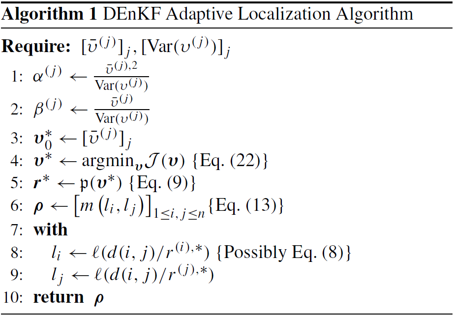
In practice, instead of dealing with the Gamma distribution parameters of α and β, we use the parameters $\overline{\mathit{\upsilon }}$ and Var(υ), such that $\mathit{\alpha }=\frac{{\overline{\mathit{\upsilon }}}^{\mathrm{2}}}{\text{Var}\left(\mathit{\upsilon }\right)}$ and $\mathit{\beta }=\frac{\overline{\mathit{\upsilon }}}{\text{Var}\left(\mathit{\upsilon }\right)}$. For the sake of simplicity we assume that all υ are identically distributed, but this is not required for the algorithm to function. The initial guess for our minimization procedure is the vector of means. After minimizing the cost function, the radii for different components will be different. These radii, along with the corresponding localization and m functions, are used to build the localization matrix ρ. An outline is presented in Algorithm 1.

5 Numerical experiments and results

In order to validate our methodology, we carry out twin experiments under the assumption of identical perfect dynamical systems for both the truth and the model. The analysis accuracy is measured by the spatio-temporally averaged root mean square error:

$$\begin{array}{}\text{(26)}& {\displaystyle }\text{RMSE}=\sqrt{{\displaystyle \frac{\mathrm{1}}{n\cdot n_t}}\sum _{i=\mathrm{1}}^{n_t}\sum _{j=\mathrm{1}}^n{\left([{\mathit{x}}_i^{\mathrm{t}}{]}_j-[{\overline{\mathit{x}}}_i^{\mathrm{a}}{]}_j\right)}^{\mathrm{2}}},\end{array}$$

where n_t is the number of data assimilation cycles (the number of analysis steps).

For each of the models we repeat the experiments with different values of the inflation constant α and report the best (minimal RMSE) results.

All initial value problems used were independently implemented (Roberts et al., 2019).

5.1 Oracles

We will make use of oracles to empirically evaluate the performance of the multivariate approach to Schur-product localization. An oracle is an idealized procedure that produces close to optimal results by making use of all the available information, some of which is unknown to the data assimilation system. In our case the oracle minimizes cost functions involving the true model state. Specifically, in an ideal filtering scenario one seeks to minimize the error of the analysis with respect to the truth, i.e., the cost function,

$$\begin{array}{}\text{(27)}& \mathcal{J}\left({\mathit{x}}^{\mathrm{a}}\right)=\text{RMSE}({\mathit{x}}^{\mathrm{a}}-{\mathit{x}}^{\mathrm{t}}).\end{array}$$

Our oracle will pick the best parameters, in this case the radii, that minimize an ideal cost function $\mathcal{J}\left(\mathit{\upsilon }\right)=\text{RMSE}({\overline{\mathit{x}}}_{\left(\mathit{\upsilon }\right)}^{\mathrm{a}}-{\mathit{x}}^{\mathrm{t}})$. This can be viewed as an ideal variance minimization of the state space in parameter space.

5.2 Lorenz'96

The 40-variable Lorenz model (Lorenz, 1996; Lorenz and Emanuel, 1998) is the first standard test employed. This problem is widely used in the testing of data assimilation algorithms.

5.2.1 Model setup

The Lorenz'96 model equations,

$$\begin{array}{}\text{(28)}& {\displaystyle \frac{\mathrm{d}{x}_i}{\mathrm{d}t}}=(x_{i+\mathrm{1}}-x_{i-\mathrm{2}})x_{i-\mathrm{1}}-x_i+F,i=\mathrm{1},\mathrm{\dots }n,\end{array}$$

are obtained through a coarse discretization of a forced Burger equation with Newtonian damping (Reich and Cotter, 2015). We impose x₀=x_n, $x_{-\mathrm{1}}=x_{n-\mathrm{1}}$, and $x_{n+\mathrm{1}}=x_{\mathrm{1}}$, where n=40. We take the canonical value for the external forcing factor, F=8. Using known techniques for dynamical systems (Parker and Chua, 2012), one can approximately compute that this particular system has 13 positive Lyapunov exponents (Strogatz, 2014) and 1 zero exponent, with a Kaplan–Yorke dimension of approximately 27.1.

The initial conditions used for the experiments are obtained by starting with

$$\begin{array}{}\text{(29)}& [{\mathit{x}}_{\mathrm{0}}{]}_i=\left\{\begin{array}{ll}\mathrm{8}& i\ne \mathrm{20}\\ \mathrm{8.008}& i=\mathrm{20}\end{array}\right.\end{array}$$

and integrating Eq. (28) forward for 1 time unit in order to reach the attractor.

The physical distance between x_i and x_j is the shortest cyclic distance between any two state variables:

$$\begin{array}{}\text{(30)}& {\displaystyle }d(i,j)=min\mathit{\{}\Vert i-j\Vert ,\Vert n+i-j\Vert ,\Vert n+j-i\Vert \mathit{\}},\end{array}$$

where the distance between two neighbors is 1.

For the numerical experiments, we consider a perfect model and noisy observations. We take a 6 h assimilation window (corresponding to Δt_obs=0.05 model time units) and calculate the RMSE on the assimilation cycle interval [100,1100] in the case of oracle testing or [5000,55 000] in the case of adaptive localization testing. Lorenz'96 is an ergodic system (Fatkullin and Vanden-Eijnden, 2004), and therefore its behavior in time for most initial conditions is the same as the behavior of all its possible phase spaces on any orbit around a strange attractor at any point in time, meaning that a long enough time averaged run should be the same as a collection of shorter space-averaged runs. We use 10 ensemble members (just under the number of positive Lyapunov exponents) and observe the 30 model variables ($\mathrm{2},\mathrm{4},\mathrm{\dots },\mathrm{18},\mathrm{20},\mathrm{21},\mathrm{\dots },\mathrm{39},\mathrm{40}$), with an observation error variance of 1 for each observed state.

5.2.2 Oracle results

Figure 1 shows a visualization of multivariate oracle runs for the Lorenz'96 test problem using the best constant radius, a univariate oracle, and a multivariate oracle utilizing the m functions from Eq. (10a). The constant “best” radius was chosen on an individual basis for every value of the inflation parameter, while the univariate and multivariate cases were allowed to minimize Eq. (27) for a single global radius and for 40 local radii, respectively. This means that in the multivariate case each of the 40 variables is given an independent radius. As one can see, the univariate oracle performs no better than a constant radius, while several of the multivariate approaches provide much better results. The schemes (Eq. 10a) that closely mirror an unbiased mean, namely m_mean, m_sqrt, m_rms, and m_harm, yield the best results, while the conservative scheme m_min performs no better than a univariate approach. This indicates that the problem is better suited for multivariate localization. Most m functions perform similarly, and in further experiments we will only consider m_mean as a representative and easy-to-implement option. We note that for Lorenz'96 with DEnKF and our experimental setup, no 3-D univariate adaptive localization scheme which aims for the analysis estimate to optimally approach the truth outperforms the best constant localization radius.

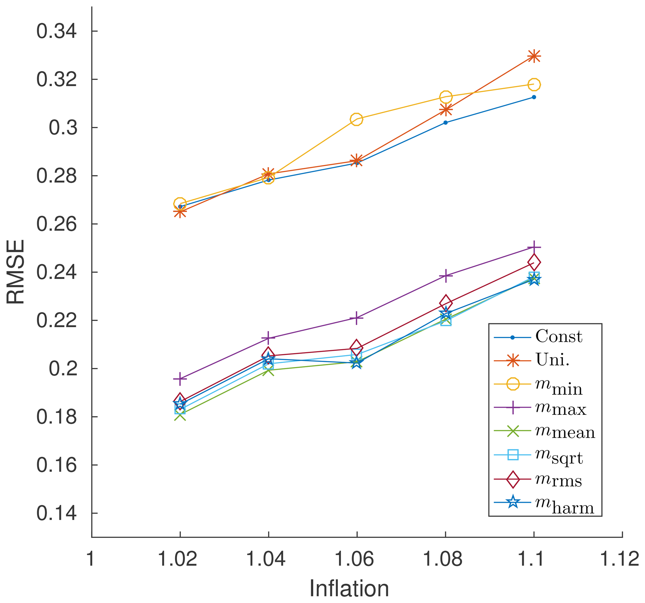
Figure 1 Generalized mean oracles for Lorenz'96. Comparison of the various m-based multivariate localization techniques with that of standard univariate localization and constant “best radius” localization. Results were obtained using the Lorenz'96 model over the assimilation cycles [100,1100] and were run for various values of the inflation parameter.

We also test both the validity of arbitrarily grouping the radii and the validity of using a time-distributed cost function (Eq. 25). Figure 2 presents results for arbitrary radii groupings and for a limited run 4-D approach. The results were calculated with arbitrary choices of radii groupings such that each group would contain an equal number of variables, and with the fixed inflation value of α=1.02 with the function m_mean. There is significant benefit in using more radii groupings, but marginal benefit from the 4-D approach.

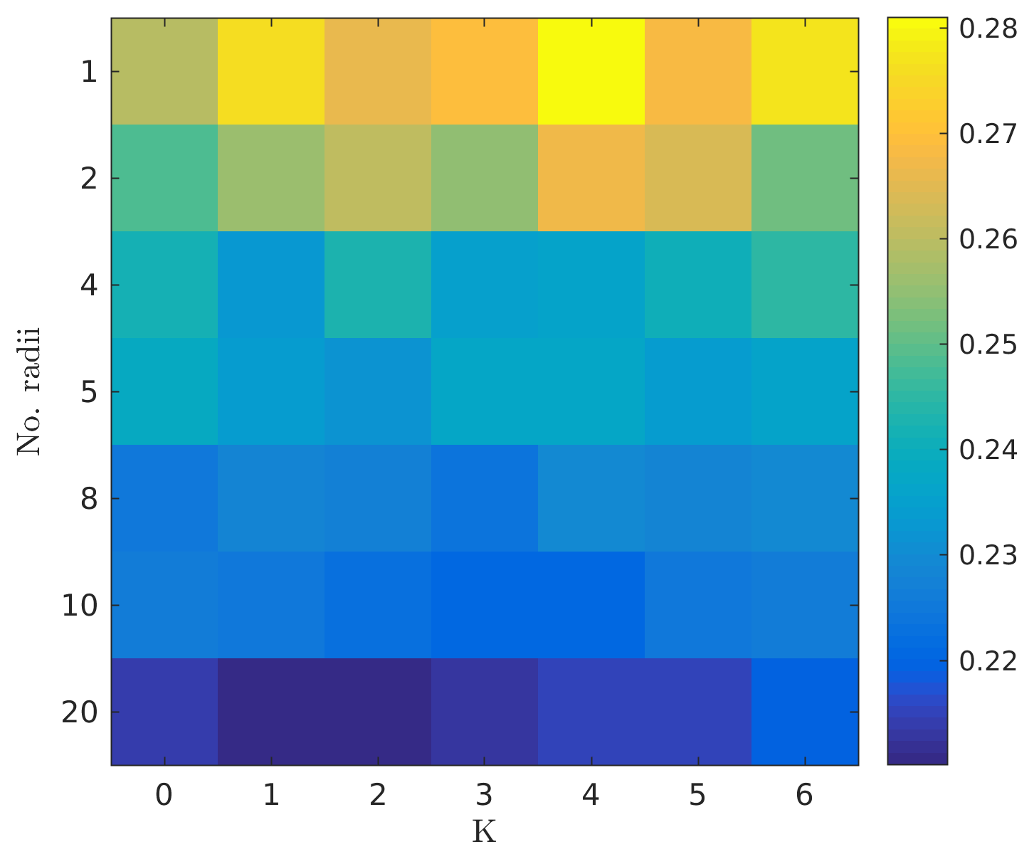
Figure 2 Time-dependent 4-D oracle for Lorenz'96. Comparison of the RMSE for a radius oracle that is both multivariate and time-dependent. The y axis represents the number of independent radii values (groups of the model state components). The assimilation cycle interval is [100,1100]; a fixed inflation value of α=1.02 and the function m_mean are used.

5.2.3 Adaptive localization results

Adaptive localization results for Lorenz'96 are shown in Fig. 3. The optimal constant localization radius was found and a search of possible input mean and variance values was performed around it for the adaptive case. The value of $\overline{\mathit{\upsilon }}$ was varied by additive factors of one of −1, −0.5, +0, +0.5, or +1 with respect to the best univariate radius with Var(υ) chosen to be one of 1∕8, 1∕4, 1∕2, 1, or 2. As accurately predicted by the oracle results, a univariate adaptive approach for this model cannot do better than the best univariate radius (Fig. 1), as no meaningful reduction in error was detected.

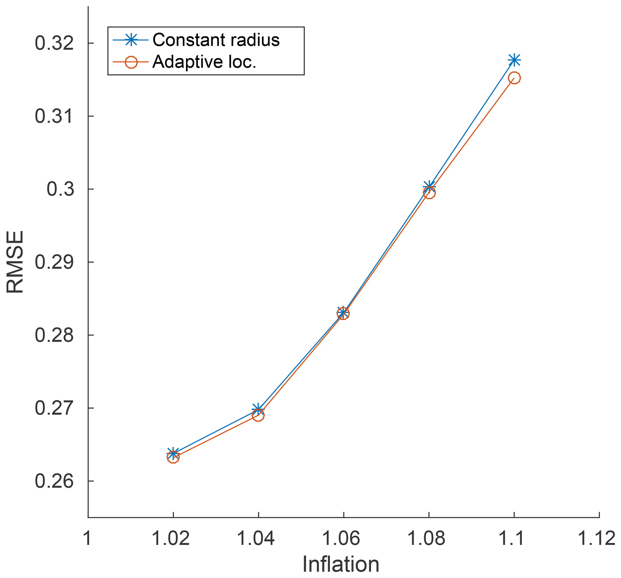
Figure 3 Lorenz'96 adaptive localization results. Comparison of the best univariate localization radius results with their corresponding adaptive localization counterparts. $\overline{\mathit{\upsilon }}$ was varied by additive factors of one of −1, −0.5, +0, +0.5, or +1 with respect to the best univariate radius, with Var(υ) chosen to be one of 1∕8, 1∕4, 1∕2, 1, or 2.

5.3 Multivariate Lorenz'96

The canonical Lorenz'96 model is ill suited for multivariate adaptive localization as each variable in the problem behaves identically to all the others. This means that for any univariate localization scheme a constant radius is close to optimal.

5.3.1 Model setup

We modify the problem in such a way that the average behavior remains very similar to that of the original model, but that instantaneous behavior requires different localization radii. In order to accomplish this we use the time-dependent forcing function that is different for each variable:

$$\begin{array}{}\text{(31)}& {\displaystyle }{\left[\mathit{F}\left(t\right)\right]}_i=\mathrm{8}+\mathrm{4}\cos \left(\mathit{\omega }\right(t+{\displaystyle \frac{(i-\mathrm{1})\mathrm{mod}q}{q}}\left)\right),\end{array}$$

where ω=2π (in the context of Lorenz'96 the equivalent period is 5 d), i is the variable index, and q is an integer factor of n. Here we set q=4. The different forcing values will create differences between the dynamics of different variables.

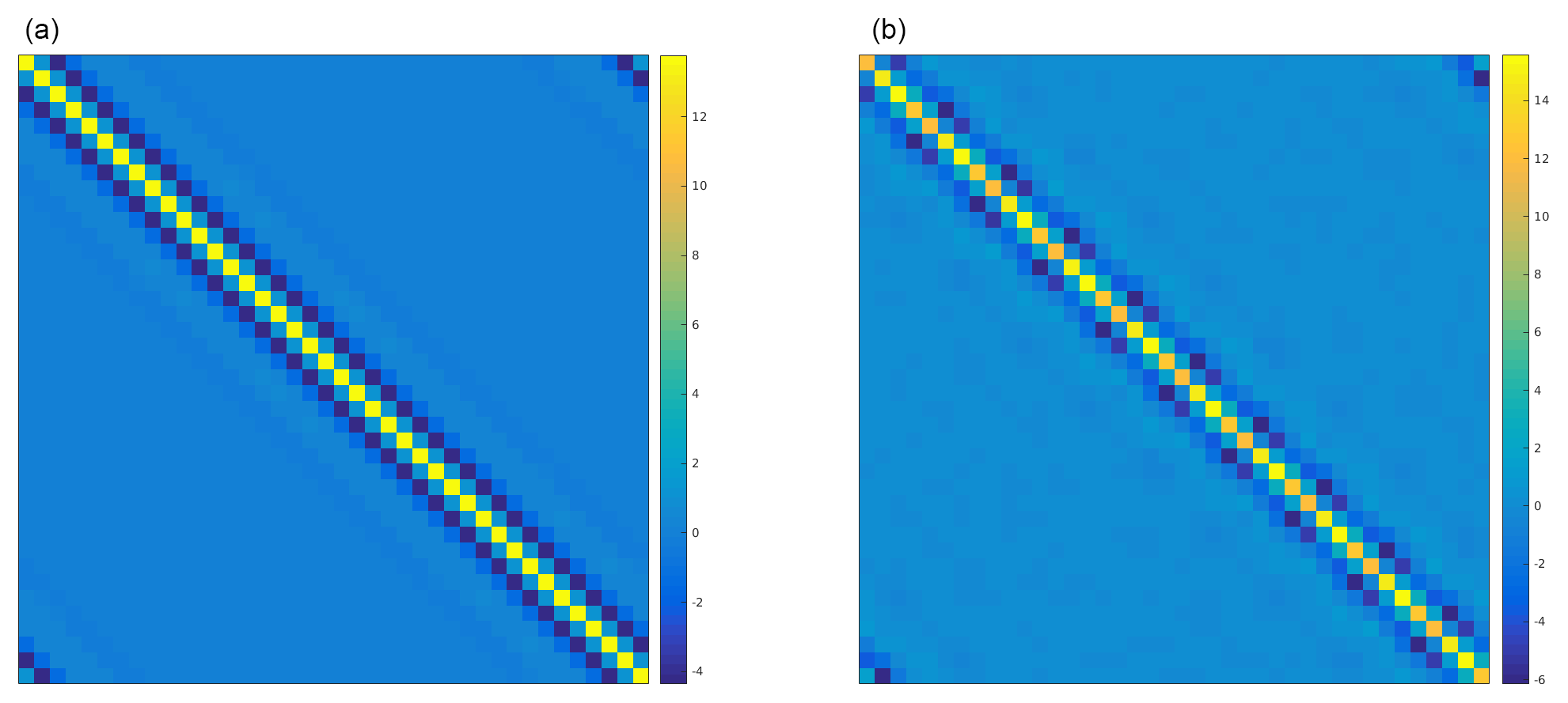
Figure 4 Calculated optimal single-time and time-averaged covariance matrices for the multivariate Lorenz'96 model. Comparison of ensemble covariance matrices for the multivariate Lorenz'96 equations for a single time step (a) with that for a time-averaged run (b) for 100 000 and 10 000 ensemble members, respectively.

For each individual variable the forcing value cycles between 4 and 12, with an average value of 8, just like in the canonical Lorenz'96 formulation. If taken to be a constant, the forcing factor of 4 will make the equation lightly chaotic with only one positive Lyapunov exponent, whilst a constant value of 12 will make the dynamics have about 15 positive Lyapunov exponents. Our modified system still has the same average behavior with 13 positive Lyapunov exponents. The mean doubling times of the two problems are also extremely similar at around 0.36. This is the ideal desired behavior. Figure 4 shows a comparison of numerically computed covariance matrices for this modified problem. There is considerable difference between the size of non-diagonal entries for different state variables over the course of a single step, but this difference disappears after averaging. This indicates that for this problem the best constant univariate radius is the same as for the canonical Lorenz'96 model but that instantaneous adaptive radii are different. This shows that an adaptive approach to the instantaneous covariance could be advantageous.

Error measurements will be carried out over the interval [500,5500], with the omitted steps acting as spinup. The rest of the problem setup is identical to that of the canonical Lorenz'96.

5.3.2 Adaptive localization results

Figure 5 shows results with the multivariate Lorenz'96 model, with $g=q=\mathrm{4}$ radii groups and the 4-D parameter set to K=1. The inflation is kept constant for each experiment, with multiple experiments spanning $\mathit{\alpha }\in [\mathrm{1.02},\mathrm{1.1}]$. The localization radius is varied in increments of 0.5 over the range [0.5,16] for the constant case. The corresponding minimal-error radii are used as mean inputs into our adaptive algorithm. For the adaptive case we choose four arbitrary groupings of radii (g=4) with the mean function m_mean. The parameters $\overline{\mathit{\upsilon }}$ take one of three possible values, the optimal constant radius −1, +0, and +1. The parameters Var(υ) take one value from $\mathit{\{}\mathrm{1}/\mathrm{4},\mathrm{1},\mathrm{4}\mathit{\}}$. The 4-D variable is set to K=1 to look at an additional observation in the future.

Figure 5 Time-dependent multivariate Lorenz'96 4-D adaptive localization. The constant radius case shows the minimal error when the localization radius is varied between set predefined values. The adaptive localization case has four radii groupings, $g=q=\mathrm{4}$, with the time-dependence parameter, K=1. The parameters $\overline{\mathit{\upsilon }}$ were varied by −1, +0, and +1 from the best constant radius. The parameters Var(υ) take one value from $\mathit{\{}\mathrm{1}/\mathrm{4},\mathrm{1},\mathrm{4}\mathit{\}}$.

As before, the results for the constant radius were their optimal value for each given inflation value, while the adaptive results were obtained through a search for possible means and variances around that value. The largest reduction in error is only about 8 %; however, this is a significant improvement over the behavior of the univariate Lorenz'96. In the canonical Lorenz'96 there is no meaningful choice of grouping other than arbitrary, but in this case, the groups were chosen such that all related variables have the same forcing from Eq. (31). The results show a significant improvement over the univariate case, especially for low inflation values. We note that the filter spinup takes significantly longer for the adaptive localization case than for the constant univariate case. Consequently, the assimilation cycles are chosen in the time interval [500,5500] units. An idea to mitigate this might be to run the filter with a constant radius for a few assimilation cycles before switching to the adaptive localization strategy, so as to allow the filter to quickly catch up with the shadow attractor trajectory.

Figure 6 demonstrates a sampling of the radii obtained through the adaptive 4-D multivariate method. Taking $g=q=\mathrm{4}$, α=1.02, $\overline{\mathit{\upsilon }}=\mathrm{6}$, Var(υ)=1, and K=1, we look at the radii generated by our method. For the post-spinup case, the means (5.8449, 5.8669, 5.8441, 5.8602) of the radii for each grouping are fairly similar; however, the variances (0.0300, 0.0731, 0.0295, 0.0821) differ wildly. The groupings with less observations, groups 1 and 3, have much more conservative variances, while groups 3 and 4, which are observed fully, have much greater variances.

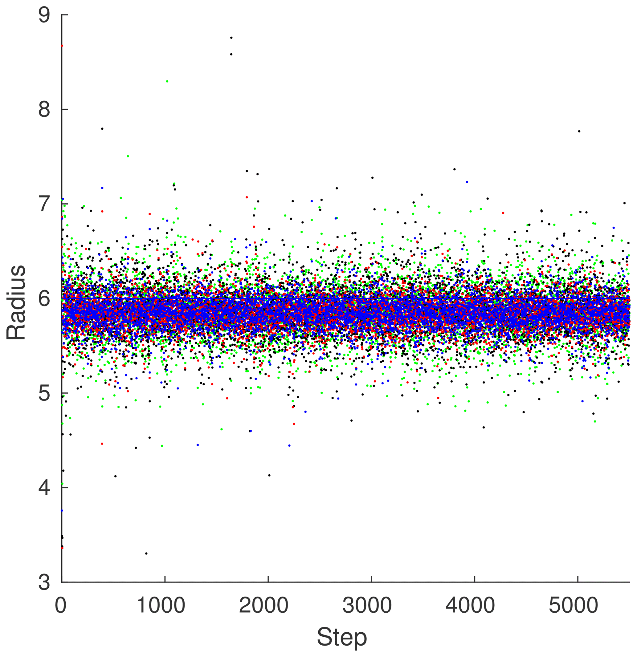
Figure 6 ML96 sample radii. Radii for the configuration in Fig. 5 with α=1.02, $\overline{\mathit{\upsilon }}=\mathrm{6}$, and Var(υ)=1. Each unique marker type represents a unique radius grouping with a red ⋅ representing the first group, a green ⋅ representing the second, a blue ⋅ representing the third, and a black ⋅ representing the fourth. Groups 2 and 4 contain variables that were observed fully, and groups 1 and 3 contain variables that were observed partially. The graph has been truncated to only show radii from 3 to 9 in order to better capture the general tendencies.

This gives us insight into a potential way of choosing multivariate localization groups. Based on some measure of the observability of any given state-space variable, similarly “observable” state-space variables should have similar radii.

Tightly coupled models like the multivariate Lorenz'96 have rapidly diverging solutions, and constraining them requires more information about the underlying dynamics. Incorporating future observations and adding degrees of freedom to the cost function increase the performance of our analysis. In the limiting case of one radius per variable and general information from the future one approaches a variant of 4DenVar, which is in principle superior to any pure filtering method.

5.4 Quasi-geostrophic model (QGSO)

The 1.5-layer quasi-geostrophic model of Sakov and Oke (Sakov and Oke, 2008), obtained by non-dimensionalizing potential vorticity, is given by the equations

$$\begin{array}{l}{\displaystyle }{q}_t=-{\mathit{\psi }}_x-\mathit{\epsilon }J(\mathit{\psi },q)-A{\mathrm{△}}^{\mathrm{3}}\mathit{\psi }+\mathrm{2}\mathit{\pi }\sin \left(\mathrm{2}\mathit{\pi }y\right),\\ \text{(32)}& {\displaystyle }\mathrm{△}\mathit{\psi }-F\mathit{\psi }=q,J(\mathit{\psi },q)\equiv {\mathit{\psi }}_x{q}_y-{\mathit{\psi }}_y{q}_x.\end{array}$$

The variable ψ can be thought of as the stream function, and the spatial domain is the square $(x,y)\in [\mathrm{0},\mathrm{1}{]}^{\mathrm{2}}$. The constants are F=1600, $\mathit{\epsilon }={\mathrm{10}}^{-\mathrm{5}}$, and $A=\mathrm{2}\times {\mathrm{10}}^{-\mathrm{11}}$. We use homogeneous Dirichlet boundary conditions.

A second-order central finite difference spatial discretization of the Laplacian operator △ is performed over the interior of a 129×129 grid, leading to a model dimension $n={\mathrm{127}}^{\mathrm{2}}=\mathrm{16}\mathrm{129}$. The time discretization is the canonical fourth-order explicit Runge–Kutta method with a time step of 1 time unit. The Helmholtz equation on the right-hand side of Eq. (32) is solved by an offline pivoted sparse Cholesky decomposition. J is calculated via the canonical Arakawa approximation (Arakawa, 1966; Ferguson, 2008). The △³ operator is implemented by repeated application of our discrete Laplacian.

The time between consecutive observations is 5 time units, and the model is run for 3300 such cycles. The first 300 cycles, corresponding to the filter spinup, are discarded, and therefore the assimilation interval is [300,3300] time units. Observations are performed with a standard 300-component observation operator as shown in Fig. 7. An observation error variance of 4 is taken for each component. The physical distance between two components is defined as

$$\begin{array}{}\text{(33)}& {\displaystyle }d(i,j)=\sqrt{(i_x-j_x{)}^{\mathrm{2}}+(i_y-j_y{)}^{\mathrm{2}}},\end{array}$$

with (i_x,i_y) and (j_x,j_y) the spatial grid coordinates of the state-space variables i and j, respectively.

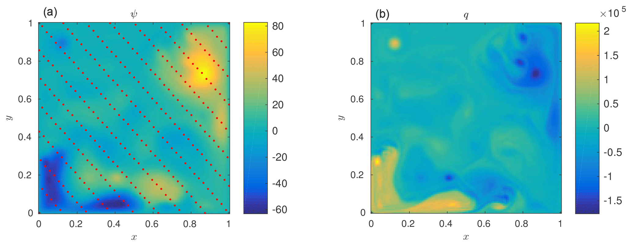
Figure 7 Quasi-geostrophic model. A typical model state of the 1.5-layer quasi-geostrophic model. (a) shows the stream function values, with the red dots representing the locations of the variables that are observed. (b) shows the corresponding vorticity.

Our rough estimate of the number of positive Lyapunov exponents of this model is 1451, with a Kaplan–Yorke dimension estimate of 6573.4; thus, we will take a conservative 25 ensemble members whose initial states are derived from a random sampling of a long run of the model.

This model has been tested extensively with both the DEnKF and various localization techniques (Sakov and Bertino, 2011; Bergemann and Reich, 2010; Moosavi et al., 2018).

Adaptive localization results

The adaptive localization results for the quasi-geostrophic problem are shown in Fig. 8. As before, a constant best univariate localization radius was calculated (iteratively taken in increments of 5 over the range [5,45]) for each inflation value ($\mathit{\alpha }\in [\mathrm{1.02},\mathrm{1.16}]$), and was used as a seed for varying the results in the adaptive case. For the adaptive case we vary the parameters $\overline{\mathit{\upsilon }}$ by taking one of three possible values, differing from the optimal constant radius by −5, 0, and +5. The adaptive Var(υ) takes one of the values 1∕2, 1, 2, or 4. An improvement of RMSE of up to about 33 % can be seen for certain inflation values, meaning that the adaptive localization procedure results in significant reductions in analysis error, while for other values no significant benefits are observed.

Figure 8 Quasi-geostrophic model adaptive localization. The inflation factor is kept constant, and α values from 1.02 to 1.16 are represented on the x axis. The constant localization radius varies in increments of 5 over the range [5,45]. Only the best results are plotted, and they are used as the mean seeds for the adaptive algorithm. For the adaptive case we vary the parameters $\overline{\mathit{\upsilon }}$ by taking one of three possible values, differing from the optimal constant radius by −5, 0, and +5. The adaptive Var(υ) takes one of the values 1∕2, 1, 2, and 4.

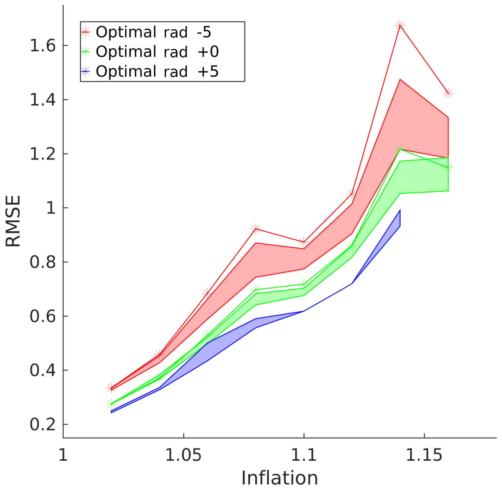
Figure 9 Quasi-geostrophic model adaptive localization raw RMSE. The green line represents the same optimal constant localization radius as in Fig. 8. The red line represents the error for the radius −5 units below, and the blue line, if it had not experienced filter divergence, would have represented +5. The correspondingly colored areas represent the ranges of error of the adaptive localization scheme obtained by fixing the mean, $\overline{\mathit{\upsilon }}$, to be that of the constant scheme and ranging over the variance.

A better representation of how well the adaptive localization scheme works is by showing its consistency. The empirical utility of the adaptive localization technique is further analyzed in Fig. 9, which compares the error results of a suboptimal constant radius with that of an adaptive run with the mean parameter set to the same values as the constant ones. The adaptive results are – except in a few cases of filter divergence – always as good as or better than their constant localization counterparts, with a reduction in error as large as 33 % with the same mean radius as the constant radius, and as much as 50 % with different radii. Even in the case where the adaptive filter diverged, the constant localization filter diverged as well. This indicates that our localization scheme is significantly better than a corresponding sub-optimal constant scheme with the same parameters, as is typically the case in real-world production codes. This opens up the possibility of adapting existing systems that use a conservative suboptimal constant localization to an adaptive localization scheme.

Figure 10 QGSO sample radii. For the configuration in Fig. 8 with α=1.08, $\overline{\mathit{\upsilon }}=\mathrm{25}$, and Var(υ)=4. Each dot represents a radius, with the line representing the mean.

Figure 10 shows a sample of the radii obtained by the adaptive algorithm. One will notice that during the spinup time the algorithm is much more conservative, with the radius of influence signaling that there should be an over-reliance on the observations instead of the model prior. After the spinup time however, the algorithm tends to select radii greater than the mean, signifying a greater confidence in the observations.

6 Conclusions

This paper proposes a novel Bayesian approach to adaptive Schur-product-based localization. A multivariate approach is developed, where multiple radii corresponding to different types of variables are taken into account. The Bayesian problem is solved by constructing 3-D and 4-D cost functions and minimizing them to obtain the maximum a posteriori estimates of the localization radii. We show that in the case of the DEnKF these cost functions and their gradients are computationally inexpensive to evaluate and can be relatively easily implemented within existing frameworks. We provide a new approach for assessing the performance of adaptive localization approaches through the use of restricted cost function oracles.

The adaptive localization approach is tested using the Lorenz'96 and quasi-geostrophic models. Somewhat surprisingly, the adaptivity produces better results for the larger quasi-geostrophic problem. This may be due to the ensemble analysis anomaly independence assumption made in Sect. 4.1, an assumption that holds better for a large system with sparse observations than for a small tightly coupled system with dense observations. The performance of the adaptive approach on the small, coupled Lorenz'96 system is increased by using multivariate and 4-D extensions of the cost function. The approach yields modest gains of about an 8 % reduction in error, but more importantly shows empirical evidence for a quite intuitive observation that variables that are more strongly observed can accept a greater variance of localization radii and can be less conservative with their radii choices.

We believe that the algorithm presented herein has a strong potential to improve existing geophysical data assimilation systems that use ensemble-based filters such as the DEnKF. In order to avoid filter divergence in the long term, these systems often use a conservative localization radius and a liberal inflation factor. The QG model results indicate that, in such cases, our adaptive method outperforms the approach based on a constant localization. The approach leads to a reduction of as much as 33 % in error. For a severely undersampled ensemble, the approach appears to improve the quality of the analysis substantially, potentially because the need for localization is significantly greater than for a small toy problem like L96. The new adaptive methodology can replace the existing approach with a relatively modest implementation effort.

Future work to extend the methodology includes finding good approximations of the probability distribution of the localization parameters, perhaps through a machine learning approach, and reducing the need for assumption that the ensemble members are independent identically distributed random variables. A future direction of interest is applying this methodology to a larger operational model, e.g., the Weather Research and Forecasting Model (WRF) (Skamarock et al., 2008), which is computationally feasible in the short term.