the Creative Commons Attribution 4.0 License.
the Creative Commons Attribution 4.0 License.
 | 12 Nov 2018
Review article: Comparison of local particle filters and new implementations
Marc Bocquet
Particle filtering is a generic weighted ensemble data assimilation method based on sequential importance sampling, suited for nonlinear and non-Gaussian filtering problems. Unless the number of ensemble members scales exponentially with the problem size, particle filter (PF) algorithms experience weight degeneracy. This phenomenon is a manifestation of the curse of dimensionality that prevents the use of PF methods for high-dimensional data assimilation. The use of local analyses to counteract the curse of dimensionality was suggested early in the development of PF algorithms. However, implementing localisation in the PF is a challenge, because there is no simple and yet consistent way of gluing together locally updated particles across domains.
In this article, we review the ideas related to localisation and the PF in the geosciences. We introduce a generic and theoretical classification of local particle filter (LPF) algorithms, with an emphasis on the advantages and drawbacks of each category. Alongside the classification, we suggest practical solutions to the difficulties of local particle filtering, which lead to new implementations and improvements in the design of LPF algorithms.
The LPF algorithms are systematically tested and compared using twin experiments with the one-dimensional Lorenz 40-variables model and with a two-dimensional barotropic vorticity model. The results illustrate the advantages of using the optimal transport theory to design the local analysis. With reasonable ensemble sizes, the best LPF algorithms yield data assimilation scores comparable to those of typical ensemble Kalman filter algorithms, even for a mildly nonlinear system.
- Article
(2406 KB) - Full-text XML
- BibTeX
- EndNote


The ensemble Kalman filter (EnKF, Evensen, 1994) and its variants are currently among the most popular data assimilation (DA) methods. Because EnKF-like methods are simple to implement, they have been successfully developed and applied to numerous dynamical systems in geophysics such as atmospheric and oceanographic models, including in operational conditions (see for example Houtekamer et al., 2005; Sakov et al., 2012a).
The EnKF can be viewed as a subclass of sequential Monte Carlo (MC) methods whose analysis step relies on Gaussian distributions. However, observations can have non-Gaussian error distributions, an example being the case of bounded variables, which are frequent in ocean and land surface modelling or in atmospheric chemistry. Most geophysical dynamical models are nonlinear yielding non-Gaussian error distributions (Bocquet et al., 2010). Moreover, recent advances in numerical modelling enable the use of finer resolutions for the models: small scale processes that can increase nonlinearity must then be resolved.
When the Gaussian assumption is not fulfilled, Kalman filtering is suboptimal. Iterative ensemble Kalman filter and smoother methods have been developed to overcome these limitations, mainly by including variational analysis in the algorithms (Zupanski, 2005; Sakov et al., 2012b; Bocquet and Sakov, 2014) or through heuristic iterations (Kalnay and Yang, 2010). Yet one cannot bypass the Gaussian representation of the conditional density with these latter methods. On the other hand, with particle filter (PF) methods (Gordon et al., 1993; Doucet et al., 2001; Arulampalam et al., 2002; Chen, 2003; van Leeuwen, 2009; Bocquet et al., 2010), all Gaussian and linear hypotheses have been relaxed, allowing a fully Bayesian analysis step. That is why the generic PF is a promising method.
Unfortunately, there is no successful application of it to a significantly high-dimensional DA problem. Unless the number of ensemble members scales exponentially with the problem size, PF methods experience weight degeneracy and yield poor estimates of the model state. This phenomenon is a symptom of the curse of dimensionality and is the main obstacle to an application of PF algorithms to most DA problems (Silverman, 1986; Kong et al., 1994; Snyder et al., 2008). Nevertheless, the PF has appealing properties – the method is elegant, simple, and fast, and it allows for a Bayesian analysis. Part of the research on the PF is dedicated to their application to high-dimensional DA with a focus on four topics: importance sampling, resampling, hybridisation, and localisation.
Importance sampling is at the heart of PF methods where the goal is to construct a sample of the posterior density (the conditional density) given particles from the prior density using importance weights. The use of a proposal transition density is a way to reduce the variance of the importance weights, hence allowing the use of fewer particles. However, importance sampling with a proposal density can lead to more costly algorithms that are not necessarily rid of the curse of dimensionality (chap. 4 of MacKay, 2003; Snyder et al., 2015). Proposal-density PF methods include the optimal importance particle filter (OIPF, Doucet et al., 2000), whose exact implementation is only available in simple DA problems (linear observation operator and additive Gaussian noise), the implicit particle filter (Chorin and Tu, 2009; Chorin et al., 2010; Morzfeld et al., 2012), which is an extension of the OIPF for DA problems using smoothing, the equivalent-weights particle filter (EWPF), and its implicit version (van Leeuwen, 2010; Zhu et al., 2016).
Resampling is the first improvement that was suggested in the bootstrap algorithm (Gordon et al., 1993) to avoid the collapse of a PF based on sequential importance sampling. Common resampling algorithms include the multinomial resampling and the stochastic universal (SU) sampling algorithms. The resampling step allows the algorithm to focus on particles that are more likely, but as a drawback, it introduces sampling noise. Worse, it may lead to sample impoverishment, hence failing to avoid the collapse of the PF if the model noise is insufficient (van Leeuwen, 2009; Bocquet et al., 2010). Therefore it is usual practice to add a regularisation step after the resampling (Musso et al., 2001). Using ideas from the optimal transport theory, Reich (2013) designed a resampling algorithm that creates strong bindings between the prior ensemble members and the updated ensemble members.
Hybridising PFs with EnKFs seems a promising approach for the application of PF methods to high-dimensional DA, in which one can hope to take the best of both worlds: the robustness of the EnKF and the Bayesian analysis of the PF. The balance between the EnKF and the PF analysis must be chosen carefully. Hybridisation especially suits the case where the number of significantly nonlinear degrees of freedom is small compared to the others. Hybrid filters have been applied, for example, to geophysical low-order models (Chustagulprom et al., 2016) and to Lagrangian DA (Apte and Jones, 2013; Slivinski et al., 2015).
In most geophysical systems, distant regions have an (almost) independent evolution over short timescales. This idea was used in the EnKF to implement localisation in the analysis (Houtekamer and Mitchell, 2001; Hamill et al., 2001; Evensen, 2003; Ott et al., 2004). In a PF context, localisation could be used to counteract the curse of dimensionality. Yet, if localisation of the EnKF is simple and leads to efficient algorithms (Hunt et al., 2007), implementing localisation in the PF is a challenge, because there is no trivial way of gluing together locally updated particles across domains (van Leeuwen, 2009). The aim of this paper is to review and compare recent propositions of local particle filter (LPF) algorithms (Rebeschini and van Handel, 2015; Lee and Majda, 2016; Penny and Miyoshi, 2016; Poterjoy, 2016; Robert and Künsch, 2017) and to suggest practical solutions to the difficulties of local particle filtering that lead to improvements in the design of LPF algorithms.
Section 2 provides some background on DA and particle filtering. Section 3 is dedicated to the curse of dimensionality, with some theoretical elements and illustrations. The challenges of localisation in PF methods are then discussed in Sects. 4 and 7 from two different angles. For both approaches, we propose new implementations of LPF algorithms, which are tested in Sects. 5, 6, and 8 with twin simulations of low-order models. Several of the LPFs are tested in Sect. 9 with twin simulations of a higher dimensional model. Conclusions are given in Sect. 10.
2.1 The data assimilation filtering problem
We follow a state vector at discrete times tk, k∈ℕ, through independent observation vectors . The evolution is assumed to be driven by a hidden Markov model whose initial distribution is p(x0), whose transition distribution is , and whose observation distribution is p(yk| xk).
The model can alternatively be described by
where the random vectors wk and vk follow the transition and observation distributions.
The components of the state vector xk are called state variables or simply variables, and the components of the observation vector yk are called observations.
Let πk|k be the analysis (or filtering) density , where yk:0 is the set , and let be the prediction (or forecast) density , with coinciding with p(x0) by convention.
The prediction operator Pk is defined by the Chapman–Kolmogorov equation:
and Bayes' theorem is used to define the correction operator Ck:
In this article, we consider the DA filtering problem that consists in estimating πk|k with given realisations of yk:0.
2.2 Particle filtering
The PF is a class of sequential MC methods that produces, from the realisations of yk:0, a set of weighted ensemble members (or particles) . The analysis density πk|k is estimated through the empirical density:
where the weights are normalised so that their sum is 1 and δx is the Dirac distribution centred at x.
Inserting the particle representation Eq. (5) in the Chapman–Kolmogorov equation yields
In order to recover a particle representation, the prediction operator Pk must be followed by a sampling step . In the bootstrap or sampling importance resampling (SIR) algorithm of Gordon et al. (1993), the sampling is performed as follows:
where x∼p means that x is a realisation of a random vector distributed according to the probability density function (pdf) p. The empirical density is now an estimator of .
Applying Bayes' theorem to gives a weight update that follows the principle of importance sampling:
The weights are then renormalised so that they sum to 1.
Finally, an optional resampling step is added if needed (see Sect. 2.3). In terms of densities, the PF can be summarised by the recursion
The additional sampling and resampling operators and are ensemble transformations that are required to propagate the particle representation of the density. Ideally, they should not alter the densities.
Under reasonable assumptions on the prediction and correction operators and on the sampling and resampling algorithms, it is possible to show that, in the limit Ne→∞, converges to πk|k for the weak topology on the set of probability measures over . This convergence result is one of the main reasons for the interest of the DA community in PF methods. More details about the convergence of PF algorithms can be found in Crisan and Doucet (2002).
Eventually, the focus of this article is on the analysis step, that is, the correction and the resampling. Hence, prior or forecast (posterior, updated, or analysis) will refer to quantities before (after) the analysis step, respectively.
2.3 Resampling
Without resampling, PF methods are subject to weight degeneracy: after a few assimilation cycles, one particle gets almost all the weight. The goal of resampling is to reduce the variance of the weights by reinitialising the ensemble. After this step, the ensemble is made of Ne equally weighted particles.
In most resampling algorithms, highly probable particles are selected and duplicated, while particles with low probability are discarded. It is desirable that the selection of particles has a low impact on the empirical density . The most common resampling algorithms – multinomial resampling, SU sampling, residual resampling, and Monte Carlo Metropolis–Hastings algorithm – are reviewed by van Leeuwen (2009). The multinomial resampling and the SU sampling algorithms, frequently mentioned in this paper, are described in Appendix E.
Resampling introduces sampling noise. On the other hand, not resampling means imparting computational time to highly improbable particles that have a very low contribution to the empirical analysis density. Therefore, the choice of the resampling frequency is critical in the design of PF algorithms. Common criteria to decide if a resampling step is needed are based on measures of the degeneracy, for example the maximum of the weights or the effective ensemble size defined by Kong et al. (1994), i.e.
The correction and resampling steps of PF methods can be combined and embedded into the so-called linear ensemble transform (LET) framework (Bishop et al., 2001; Reich and Cotter, 2015) as follows. Let Ek be the ensemble matrix, that is, the Nx×Ne matrix whose columns are the ensemble members . The update of the particles is then given by
where T is a Ne×Ne transformation matrix whose coefficients are uniquely determined during the resampling step. In the general LET framework, T has real coefficients, and it is subject to the normalisation constraint
such that the updated ensemble members can be interpreted as weighted averages of the prior ensemble members. The transformation is said to be first-order accurate if it preserves the ensemble mean (Acevedo et al., 2017), i.e. if
In the “select and duplicate” resampling schemes, the coefficients of T are in {0, 1}, meaning that the updated particles are copies of the prior particles. The first-order condition Eq. (14) is then only satisfied on average over realisations of the resampling step. Yet it is sufficient to ensure the weak convergence of almost surely in the case of the multinomial resampling (Crisan and Doucet, 2002).
If the coefficients of T are positive reals, the transformation can be understood as a resampling where the updated particles are composite copies of the prior particles. For example, in the ensemble transform particle filter (ETPF) algorithm of Reich (2013), the transformation is chosen such that it minimises the expected distance between the prior and the updated ensembles (seen as realisations of random vectors) among all possible first-order accurate transformations. This leads to a minimisation problem typical of the discrete optimal transport theory (Villani, 2009):
where 𝒯 is the set of Ne×Ne transformation matrices satisfying Eqs. (13) and (14). In this way, the correlation between the prior and the updated ensembles is increased, and still converges toward πk|k for the weak topology. In the following, this resampling algorithm will be called optimal ensemble coupling.
2.4 Proposal-density particle filters
Let q(xk+1) be a density whose support is larger than that of , i.e. whenever . The Chapman–Kolmogorov Eq. (3) can be written as
In the importance sampling literature, q is called the proposal density and can be used to perform the sampling step described by Eqs. (7) and (8) in a more general way:
Using the proposal density q can lead to an improvement of the PF method if, for example, q is easier to sample from than p or if q includes information about xk or yk+1 in order to reduce the variance of the importance weights.
The SIR algorithm is recovered with the standard proposal , while the optimal importance proposal yields the optimal importance sampling importance resampling (OISIR) algorithm (Doucet et al., 2000). Merging the prediction and correction steps of the OISIR algorithm yields the weight update
It is remarkable that this formula does not depend on xk+1 (Doucet et al., 2000). Hence the optimal importance proposal is optimal in the sense that it minimises the variance of the weights over realisations of – namely 0. Moreover, it can be shown that it also minimises the variance of the weights over realisations of the whole trajectory among proposal densities that depend on xk and yk+1 (Snyder et al., 2015).
Although the optimal importance proposal has appealing properties, its computation is non-trivial. For the generic model with Gaussian additive noise described in Appendix A2, when the observation operator ℋ is linear, the optimal importance proposal can be computed as a Kalman filter analysis as shown by Doucet et al. (2000). However, in the general case, there is no analytic form, and one must resort to more elaborate algorithms (Chorin and Tu, 2009; Chorin et al., 2010; Morzfeld et al., 2012).
3.1 The weight degeneracy of particle filters
The PF has been successfully applied to low-dimensional DA problems (Doucet et al., 2000). However, attempts to apply the SIR algorithm to medium- to high-dimensional geophysical models have led to weight degeneracy (e.g. van Leeuwen, 2003; Zhou et al., 2006).
Bocquet et al. (2010) demonstrated weight degeneracy in low-order models, for example, in the Lorenz 1996 (L96, Lorenz and Emanuel, 1998) model in the standard configuration described in Appendix A3. They illustrated the empirical statistics of the maximum of the weights for several values of the system size. When the system size is small (10 to 20 variables), weights are balanced, and values close to 1 are infrequent. However, when the system size grows (more than 40 variables) weights rapidly degenerate: values close to 1 become more frequent. Ultimately, the frequency of the maximum of the weights peaks to 1.
Similar results are produced when applying one importance sampling step to the Gaussian linear model described in Appendix A1. For this model, we illustrate the empirical statistics of the maximum of the weights in Fig. 1. Snyder et al. (2008) also computed the required number of particles in order to avoid degeneracy in simulations and found that it scales exponentially with the size of the problem.
This phenomenon, well known in the PF literature, is often referred to as degeneracy, collapse, or impoverishment and is a symptom of the curse of dimensionality.
3.2 The equivalent state dimension
At first sight, it might seem surprising that, although MC methods have a convergence rate independent of the dimension, the curse of dimensionality applies to PF methods. Yet the correction step Ck is an importance sampling step between the prior and the analysis probability densities. The higher the number of observations Ny, the more singular these densities are to each other: random particles from the prior density have an exponentially small likelihood according to the analysis density. This is the main reason for the blow-up of the number of particles required for a non-degenerate scenario (Rebeschini and van Handel, 2015).
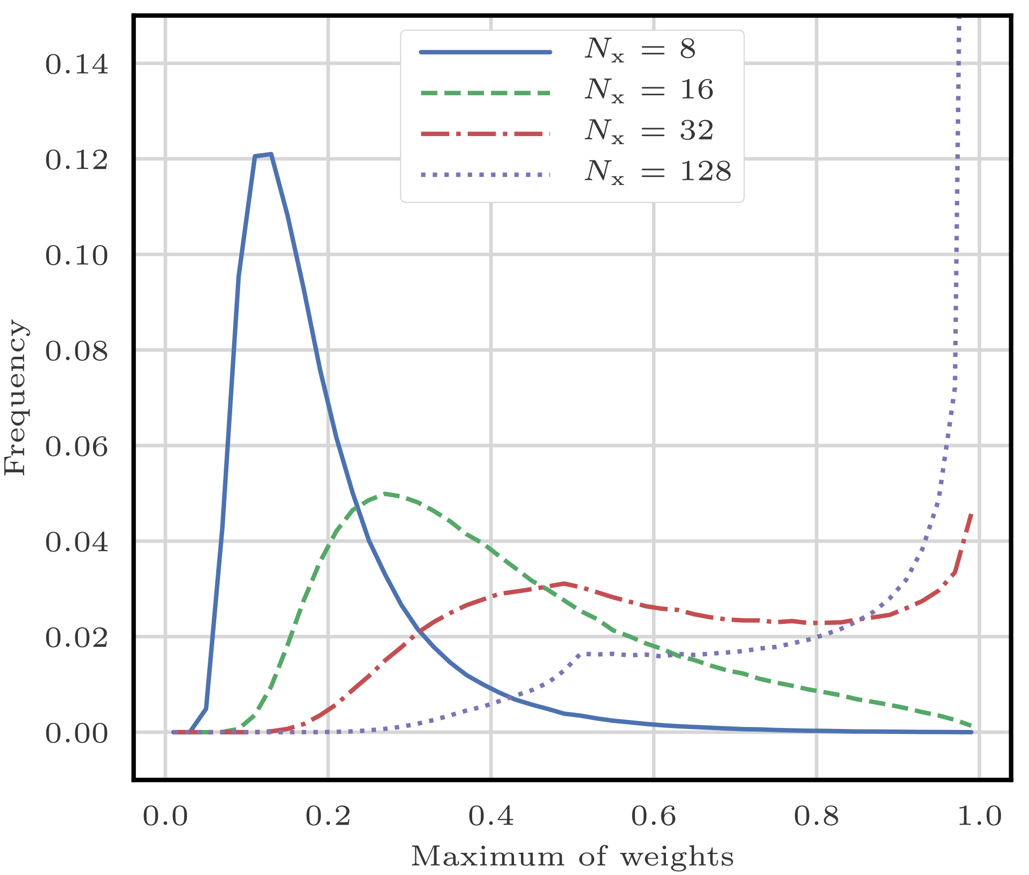
Figure 1Empirical statistics of the maximum of the weights for one importance sampling step applied to the Gaussian linear model of Appendix A1. The model parameters are p=1, a=1, h=1, q=1, and σ=1, the ensemble size is Ne=128, and the system size varies from Nx=8 (well-balanced case) to Nx=128 (almost degenerate case).
A quantitative description of the behaviour of weights for large values of Ny can be found in Snyder et al. (2008). In this study, the authors first define
with the hypothesis that the observation noise is additive and each of its components are independent and identically distributed (iid). Then they derive the asymptotic relationship for only one analysis step:
where 𝔼 is the expectation over realisations of the prior ensemble members.
This result means that, in order to avoid the collapse of a PF method, the number of particles Ne must be of order exp (τ2∕2). In simple cases, as the ones considered in the previous sections, τ2 is proportional to Ny. The dependence of τ on Nx is indirect in the sense that the derivation of Eq. (21) requires Nx to be asymptotically large. In a sense, one can think of τ2 as an equivalent state dimension.
Snyder et al. (2008) then illustrate the validity of the asymptotic relationship Eq. (21) using simulations of the Gaussian linear model of Appendix A1 with a SIR algorithm, for which
Snyder et al. (2008) do not illustrate the validity of Eq. (21) in more general cases, mainly because the computation of τ is non-trivial. The effect of resampling is not investigated either, though it is clear from simulations that resampling is not enough to avoid filter collapse. Finally, the effect of using proposal densities is the subject of another study by Snyder et al. (2015).
3.3 Mitigating the collapse using proposals
One objective of using proposal densities in PF methods is to reduce the variance of the importance weights as discussed in Sect. 2.4. If one uses the optimal importance proposal density to sample xk in the prediction and sampling step , the correction step Ck+1 consists in matching two identical densities, which leads to a weight update Eq. (19) that does not depend on the realisation of xk+1.
Yet the OISIR algorithm still collapses even for low-order models, such as the L96 model with 40 variables (Bocquet et al., 2010). In fact, the curse of dimensionality for any proposal-density PF does not primarily come from the correction step Ck, but from the recursion in the PF. In particular it stems from the fact that the algorithm does not correct the particles at earlier times to account for new observations (Snyder et al., 2015). This was a key motivation in the development of the guided SIR algorithm of van Leeuwen (2009), whose ideas were included in the practical implementations of the EWPF algorithm (van Leeuwen, 2010; Ades and van Leeuwen, 2015) as a relaxation step, with moderate success (Browne, 2016).
Snyder et al. (2015) illustrate the validity of Eq. (21) using simulations of the Gaussian linear model of Appendix A1 with an OISIR algorithm, for which
and they found a good accuracy of Eq. (21) in the limit . This shows that the use of the optimal importance proposal reduces the number of particles required to avoid the collapse of a PF method. However, ultimately, proposal-density PFs cannot counteract the curse of dimensionality in this simple model, and there is no reason to think that they could in more elaborate models (see chap. 29 of MacKay, 2003).
In a generic Gaussian linear model, the equivalent state dimension τ2 as in Eqs. (22) and (23) is directly proportional to the system size Nx, equal to Ny in this case. For more elaborate models, the relationship between τ2 and Nx is likely to be more complex and may involve the effective number of degrees of freedom in the model.
3.4 Using localisation to avoid collapse
By considering the definition of τ2 from Eq. (20), one can see that the curse of dimensionality is a consequence of the fact that the importance weights are influenced by all components of the observation vector yk. Yet a particular state variable and observation can be nearly independent, for example in spatially extended models if they are distant to each other. In this situation, the statistical properties of the ensemble at this state variable (i.e. the marginal density) should not evolve during the analysis step. Yet this is not the case in PF methods because of the use of (relatively) low ensemble sizes; even the ensemble mean can be significantly impacted. A good illustration of this phenomenon can be found in Fig. 2 of Poterjoy (2016). In this case, the PF overestimates the information available and equivalently underestimates the uncertainty in the analysis density (Snyder et al., 2008). As a consequence, spurious correlations appear between distant state variables.
This would not be the case in a PF algorithm that would be able to perform local analyses, that is, when the influence of each observation is restricted to a spatial neighbourhood of its location. The equivalent state dimension τ2 would then be defined using the maximum number of observations that influence a state variable, which could be kept relatively small even for high-dimensional systems.
In the EnKF literature, this idea is known as domain localisation or local analysis and was introduced to fix the same kind of issues (Houtekamer and Mitchell, 2001; Hamill et al., 2001; Evensen, 2003; Ott et al., 2004). The technical implementations of domain localisation in EnKF methods are as easy as implementing a global analysis, and the local analyses can be carried out in parallel (Hunt et al., 2007). By contrast, the application of localisation techniques in PF methods is discussed in Snyder et al. (2008), van Leeuwen (2009), and Bocquet et al. (2010), with an emphasis on two major difficulties.
The first issue is that the variation of the weights across local domains irredeemably breaks the structure of the global particles. There is no trivial way of recovering this global structure, i.e. gluing together the locally updated particles. Global particles are required for the prediction and sampling step in all PF algorithms, where the model ℳk is applied to each individual ensemble member.
Second, if not carefully constructed, this gluing together could lead to balance problems and sharp gradients in the fields (van Leeuwen, 2009). In EnKF methods, these issues are mitigated by using smooth functions to taper the influence of the observations. The smooth dependency of the analysis ensemble on the observation precision reduces imbalance (Greybush et al., 2011). Yet, in most PF algorithms, there is no such smooth dependency. From now on, this issue will be called “imbalance” or “discontinuity” issue. The word “discontinuity” does not point to the discrete nature of the model field on the grid, but inspired by the mathematical notion of continuity, it points to large unphysical gaps appearing in the discrete model field.
3.5 Two types of localisation
From now on, we will assume that our DA problem has a well-defined spatial structure:
-
Each state variable is attached to a location, the grid point.
-
Each observation is attached to a location, the observation site, or simply the site (observations are assumed local).
-
There is a distance function between locations.
The goal is to be able to define notions such as “the distance between an observation site and a grid point”, “the distance between two grid points”, or “the centre of a group of grid points”. In realistic models, these concepts need to be related to the underlying physical space.
In the following sections, we discuss algorithms that address the two issues of local particle filtering (gluing and imbalance) and lead to implementations of domain localisation in PF methods. We divide the solutions into two categories.
In the first approach, independent analyses are performed at each grid point by using only the observation sites that influence this grid point. This leads to algorithms that are easy to define, to implement, and to parallelise. However, there is no obvious relationship between state variables, which could be problematic with respect to the imbalance issue. This approach is used for example by Rebeschini and van Handel (2015), Penny and Miyoshi (2016), Lee and Majda (2016), and Chustagulprom et al. (2016). In this article, we call it state–domain (and later state–block–domain) localisation.
In the second approach, an analysis is performed at each observation site. When assimilating the observation at a site, we partition the state space: nearby grid points are updated, while distant grid point remain unchanged. In this formalism, observations need to be assimilated sequentially, which makes the algorithms harder to define and to parallelise but may mitigate the imbalance issue. This approach is used, for example, by Poterjoy (2016). In this article, we call it sequential–observation localisation.
From now on, the time subscript k is systematically dropped for clarity, and the conditioning with respect to prior quantities is implicit. The superscript i∈{1…Ne} is the member index, the subscript n∈{1…Nx} is the state variable or grid point index, the subscript q∈{1…Ny} is the observation or observation site index, and the subscript b∈{1…Nb} is the block index (the concept of block is defined in Sect. 4.2).
4.1 Introducing localisation in particle filters
Localisation is generally introduced in PF methods by allowing the analysis weights to depend on the spatial position. In the (global) PF, the marginal of the analysis density for each state variable is
whose localised version is
The local weights depend on the spatial position through the grid point index n.
With local analysis weights, the marginals of the analysis density are uncoupled. This is the reason why localisation was introduced in the first place, but as a drawback, the full analysis density is not known. The simplest fix is to approximate the full density as the product of its marginals:
which is a weighted sum of the possible combinations between all particles.
In summary, in LPF methods, we keep the generic MC structure described in Sect. 2.2. The prediction and sampling step is not modified. The correction step is adjusted to allow the analysis density to have the form given by Eq. (26). In particular, one has to define the local analysis weights ; this point will be discussed in Sect. 4.2.2. Finally, global particles are required for the next assimilation cycle, and they are obtained as follows. A local resampling is first performed independently for each grid point. The locally resampled particles are then assembled into global particles. The local resampling step is discussed in detail in Sect. 4.4.
4.2 Extension to state–block–domain localisation
The principle of localisation in the PF, in particular Eq. (26), can be included into a more general state–block–domain (SBD) localisation formalism. The state space is divided into (local state) blocks with the additional constraint that the weights should be constant over the blocks. The resampling then has to be performed independently for each block.
In the block particle filter algorithm of Rebeschini and van Handel (2015), the local weight of a block is computed using the observation sites that are located inside this block. However, in general, nothing prevents one from using the observation sites inside a local domain potentially different from the block. This is the case in the LPF of Penny and Miyoshi (2016), in which the blocks have size 1 grid point, while the size of the local domains is controlled by a localisation radius.
To summarise, LPF algorithms using the SBD localisation formalism, hereafter called LPFx algorithms1, are characterised by
-
the geometry of the blocks over which the weights are constant;
-
the local domain of each block, which gathers all observation sites used to compute the local weight;
-
the local resampling algorithm.
Most LPFs (e.g. those described in Rebeschini and van Handel, 2015; Penny and Miyoshi, 2016; Lee and Majda, 2016) in the literature can be seen to adopt this SBD formalism.
4.2.1 The local state blocks
Using parallelepipedal blocks is a standard geometric choice (Rebeschini and van Handel, 2015; Penny and Miyoshi, 2016). It is easy to conceive and to implement, and it offers a potentially interesting degree of freedom: the block shape. Using larger blocks decreases the proportion of block boundaries, hence the bias in the local analyses. On the other hand, it also means less freedom to counteract the curse of dimensionality.
In the clustered particle filter algorithms of Lee and Majda (2016), the blocks are centred around the observation sites. The potential gains of this method are unclear. Moreover, when the sites are regularly distributed over the space – which is the case in the numerical examples of Sects. 5 and 6 – there is no difference with the standard method.
4.2.2 The local domains
The general idea of domain localisation in the EnKF is that the analysis at one grid point is computed using only the observation sites that lie within a local region around this grid point, hereafter called the local domain. For instance, in two dimensions, a common choice is to define the local domain of a grid point as a disk, which is centred at this grid point and whose radius is a free parameter called the localisation radius. The same principle can be applied to the SBD localisation formalism: the local domain of a block will be a disk whose centre coincides with that of the block and whose radius will be a free parameter.
The terminology adopted here (disk, radius, etc.) fits two-dimensional spatial spaces. Yet most geophysical models have a three-dimensional spatial structure, with typical uneven vertical scales that are usually much shorter than horizontal scales. For these models, the geometry of the local domains should be adapted accordingly.
Increasing the localisation radius allows one to take more observation sites into account, hence reducing the bias in the local analysis. It is also a means to reduce the spatial inhomogeneity by making the weights smoother in space.
The smoothness of the local weights is an important property. Indeed, spatial discontinuities in the weights can lead to spatial discontinuities in the updated particles. Again lifting ideas from the local EnKF methods, the smoothness of the weights can be improved by tapering the influence of an observation site with respect to its distance to the block centre as follows. For the (global) PF, assuming that the observation sites are independent, the unnormalised weights are computed according to
Following Poterjoy (2016), for an LPF, it becomes
where α is a constant that should be of the same order as the maximum value of p(y| x), dq, b is the distance between the qth observation site and the centre of the bth block, r is the localisation radius, and G is the taper function: G(0)=1 and G(x)=0 if x is larger than 1, with a smooth transition. A popular choice for G is the piecewise rational function of Gaspari and Cohn (1999), hereafter called the Gaspari–Cohn function. If the observation error is an iid Gaussian additive noise with variance σ2, one can use an alternative “Gaussian” formula for , directly inspired from local EnKF methods:
Equations (28) and (29) differ. Still they are equivalent in the asymptotic limit r→0 and σ→∞.
4.2.3 Algorithm summary
Algorithm 1 describes the analysis step for a generic LPFx. The algorithm parameters are the ensemble size Ne, the geometry of the blocks, and the localisation radius r used to compute the local weights with Eq. (28) or (29). Nb is the number of blocks, and E|b is the restriction of the ensemble matrix E to the bth block (i.e. the rows of E corresponding to grid points that are located within the bth block). E|b is a matrix.
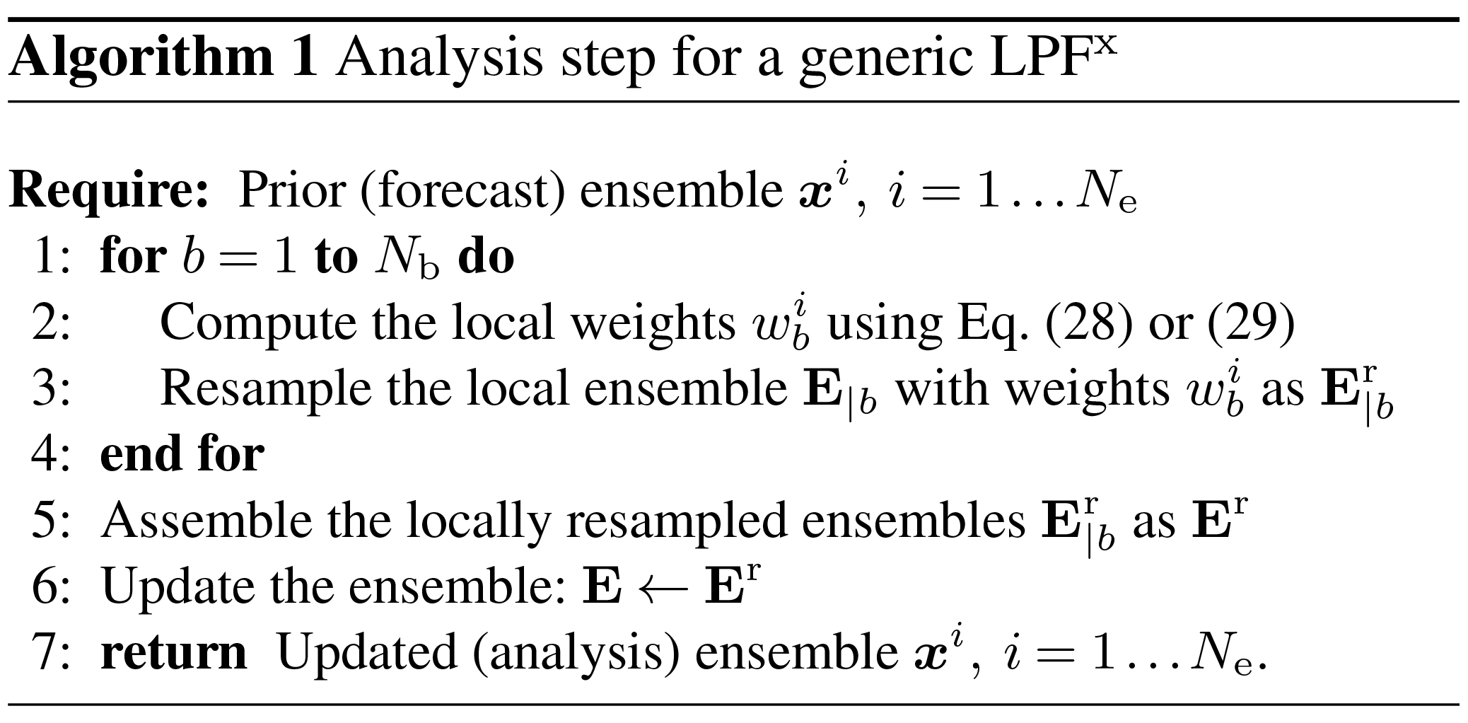
In this algorithm, and in the rest of this article, the ensemble matrix E and the particles xi (its columns) are used interchangeably. Note that in most cases, steps 3, 5, and 6 can be merged into one step.
An illustration of the definition of blocks and local domains is displayed in Fig. 2.
4.3 Beating the curse of dimensionality
The feasibility of PF methods using SBD localisation is discussed by Rebeschini and van Handel (2015) through the example of their block particle filter algorithm. In this algorithm, the distinction between blocks and local domains does not exist. The influence of each observation is not tapered and the resampling is performed independently for each block, regardless of the boundaries between blocks.
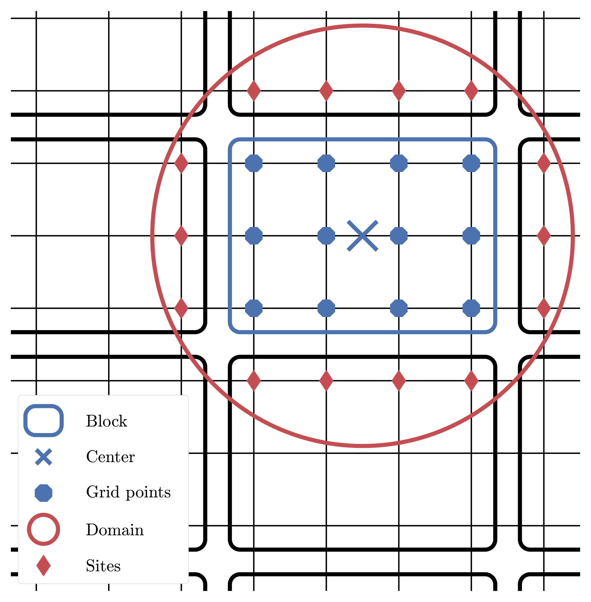
Figure 2Example of geometry in the SBD localisation formalism for a two-dimensional space. The focus is on the block in the middle, which gathers 12 grid points. The local domain is circumscribed by a circle around the block centre, with potential observation sites outside the block.
The main mathematical result is that, under reasonable hypotheses, the error on the analysis density for this algorithm can be bounded by the sum of a bias and a variance term. The bias term is related to the block boundaries and decreases exponentially with the diameter of the blocks, in number of grid points. It is due to the fact that the correction is not Bayesian anymore, since only a subset of observations is used to update each block. The exponential decrease is a demonstration of the decay of correlations property. The variance term is common to all MC methods and scales with . For global MC methods, K is the state dimension, whereas here K is the number of grid points inside each block. This implies that LPFx algorithms can indeed beat the curse of dimensionality with reasonably large ensembles.
4.4 The local resampling
Resampling from the analysis density given by Eq. (26) does not cause any theoretical or technical issue. One just needs to apply any resampling algorithm (e.g. those described in Sect. 2.3) locally to each block, using the local weights. Global particles are then obtained by assembling the locally resampled particles. By doing so, adjacent blocks are fully uncoupled – this is the same remark as when we constructed the analysis density Eq. (26) from its marginals Eq. (25). Once again, this is beneficial, since uncoupling is what counteracts the curse of dimensionality.
On the other hand, blind assembling is likely to lead to unphysical discontinuities in the updated particles, regardless of the spatial smoothness of the analysis weights. More precisely, one builds composite particles: that is when the ith updated particle is composed of the jth particle on one block and of the kth particle on an adjacent block with j≠k, as shown by Fig. 3 in one dimension. There is no guarantee that the jth and the kth local particles are close and that assembling them will represent a physical state.
In order to mitigate the unphysical discontinuities, the analysis weights must be spatially smooth, as mentioned in Sect. 4.2.2. Moreover, the resampling scheme must have some “regularity”, in order to preserve part of the spatial structure held in the prior particles. This is a challenge due to the stochastic nature of the resampling algorithms; potential solutions are presented hereafter.
4.4.1 Applying a smoothing-by-weights step
A first solution is to smooth out potential unphysical discontinuities by averaging in space the locally resampled ensemble as follows. This method was introduced by Penny and Miyoshi (2016) in their LPF and called smoothing by weights.
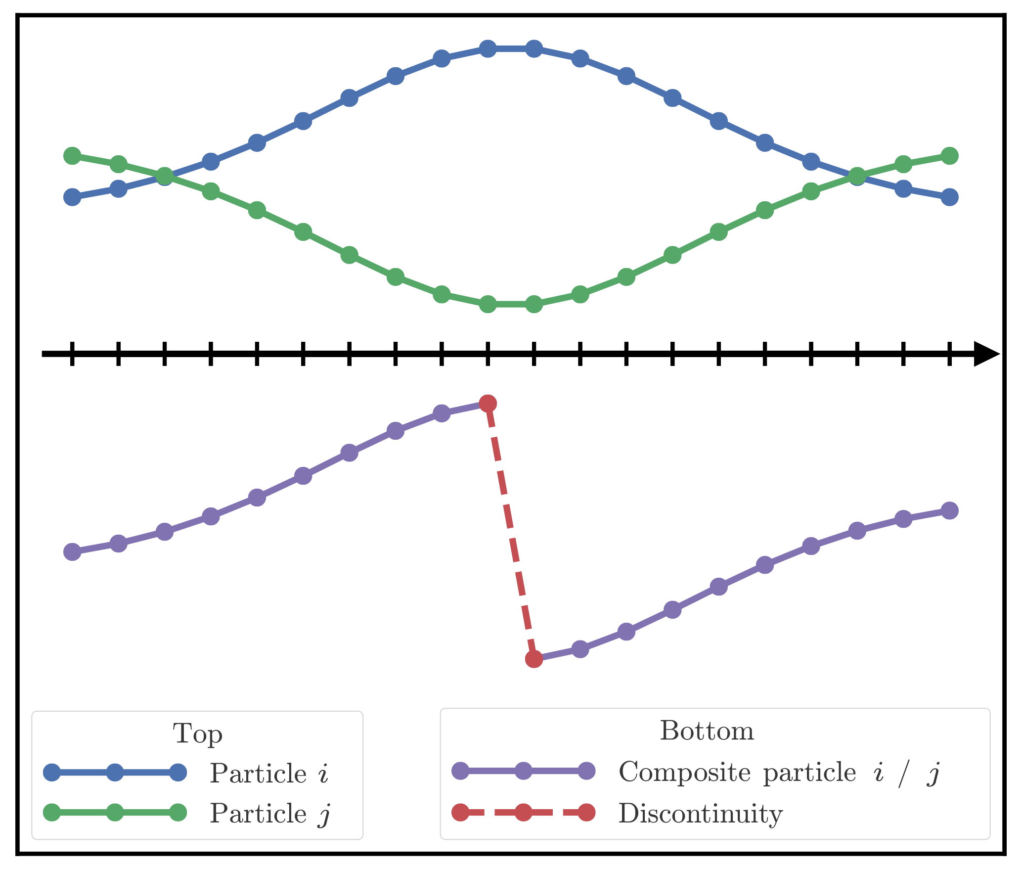
Figure 3Example of one-dimensional concatenation of particle i on the left and particle j on the right. The composite particle (purple) is a concatenation of particles i (blue) and j (green). In this situation, a large unphysical discontinuity appears at the boundary.
Let be the matrix of the ensemble computed by applying the resampling method to the global ensemble, weighted by the local weights of the bth block. is an Nx×Ne matrix different from the matrix defined in Sect. 4.2.3. We then define the smoothed ensemble matrix Es by
where dn, b is the distance between the nth grid point and the centre of the bth block, rs is the smoothing radius, a free parameter potentially different from r, and G is a taper function, potentially different from the one used to compute the local weights.
If the resampling is performed using a “select and duplicate” algorithm (see Sect. 2.3), for example, the SU sampling algorithm, then define ϕb as the resampling map for the bth block, i.e. the map computed with the local weights such that ϕb(i) is the index of the ith selected particle. With E being the prior ensemble matrix, Eq. (30) becomes
Finally, the ensemble is updated as
where Er is the resampled ensemble matrix implicitly defined by step 5 of Algorithm 1, and αs is the smoothing strength, a free parameter in [0, 1] that controls the intensity of the smoothing. When αs=0, no smoothing is performed, and when αs=1, the analysis ensemble is totally replaced by the smoothed ensemble.
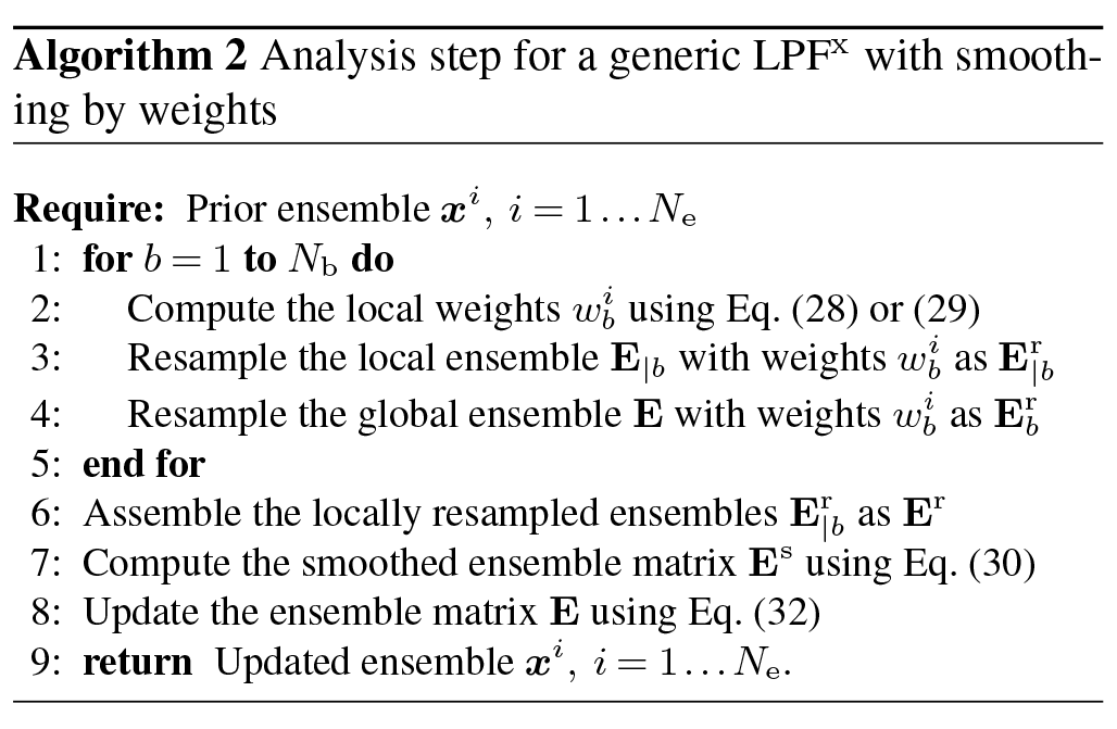
Algorithm 2 describes the analysis step for a generic LPFx with the smoothing-by-weights method. The original LPF of Penny and Miyoshi (2016) can be recovered if the following conditions are satisfied:
-
Blocks have size 1 grid point (hence there is no distinction between grid points and blocks).
-
The local weights are computed using Eq. (29).
-
The function G is a top-hat function.
-
The resampling method is the SU sampling algorithm.
-
The smoothing radius rs is set to be equal to r.
-
The smoothing strength αs is set to 0.5.
The method described here is a generalisation of their algorithm.
Note that when the resampling method is the SU sampling algorithm, the matrices do not need to be explicitly computed. One just has to store the resampling maps in memory and then use Eq. (31) to obtain the smoothed ensemble matrix Es.
The smoothing-by-weights step is an ad hoc fix to reduce potential unphysical discontinuities after they have been introduced in the local resampling step. Its necessity hints that there is room for improvement in the design of the local resampling algorithms.
4.4.2 Refining the sampling algorithms
In this section, we study several properties of the local resampling algorithm that might help dealing with the discontinuity issue: balance, adjustment, and random numbers.
A “select and duplicate” sampling algorithm is said to be balanced if, for i=1…Ne, the number of copies of the ith particle selected by the algorithm does not differ by more than one unity from wiNe. For example, this is the case of the SU sampling but not the multinomial resampling algorithm.
A “select and duplicate” sampling algorithm is said to be adjustment-minimising if the indices of the particles selected by the algorithm are reordered to maximise the number of indices i∈{1…Ne}, such that the ith updated particle is a copy of the ith original particle. The SU sampling and the multinomial resampling algorithms can be simply modified to yield adjustment-minimising resampling algorithms.
While performing the resampling independently for each block, one can use the same random number(s) in the local resampling of each block.
Using the same random number(s) for the resampling of all blocks avoids a stochastic source of unphysical discontinuity. Choosing balanced and adjustment-minimising resampling algorithms is an attempt to include some kind of continuity in the map {local weights}↦{locally updated particles} by minimising the occurrences of composite particles. However, these properties cannot eliminate all sources of unphysical discontinuity. Indeed, ultimately, composite particles will be built – if not, then localisation would not be necessary – and there is no mechanism to reduce unphysical discontinuities in them. These properties have been first introduced in the “naive” local ensemble Kalman particle filter of Robert and Künsch (2017).
4.4.3 Using optimal transport in ensemble space
As mentioned in Sect. 2.3, using the optimal transport (OT) theory to design a resampling algorithm was first investigated in the ETPF algorithm of Reich (2013).
Applying optimal ensemble coupling to the SBD localisation frameworks results in a local LET resampling method, whose local transformation at each block Tb solves the discrete OT problem
where 𝒯b is the set of Ne×Ne transformations satisfying the normalisation constraint Eq. (13) and the local first-order accuracy constraint
In the ETPF, the coefficients ci, j were chosen as the squared L2 distance between the whole ith and jth particles as in Eq. (15). Since we perform a local resampling step, it seems more appropriate to use a local criterion, such as
where dn, b is the distance between the nth grid point and the centre of the bth block, rd is the distance radius, another free parameter, and G is a taper function, potentially different from the one used to compute the local weights.
To summarise, Algorithm 3 describes the analysis step for a generic LPFx that uses optimal ensemble coupling as local resampling algorithm. Localisation was first included in the ETPF algorithm by Cheng and Reich (2015), in a similar way to the SBD localisation formalism. Hence Algorithm 3 can be seen as a generalisation of the local ETPF of Cheng and Reich (2015) that includes the concept of local state blocks.
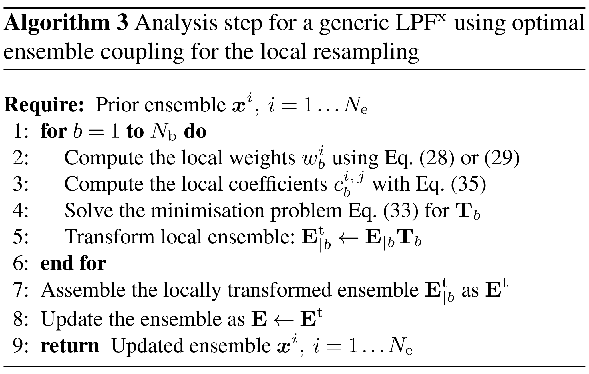
On each block, the linear transformation establishes a strong connection between the prior and the updated ensembles. Moreover, there is no stochastic variation of the coupling at each block. This means that the spatial coherence can be (at least partially) transferred from the prior to the updated ensemble.
4.4.4 Using optimal transport in state space
In Sect. 4.4.3, the discrete OT theory was used to compute a linear transformation between the prior and the updated ensembles. Following these ideas, we would like to use OT directly in state space. In more than one spatial dimension, the continuous OT problem is highly non-trivial and numerically challenging (Villani, 2009). Therefore, we will restrict ourselves to the case where blocks have size 1 grid point. Hence there is no distinction between blocks and grid points.
For each state variable n, we define the prior (marginal) pdf as the empirical density of the unweighted prior ensemble and the analysis pdf as the empirical density of the prior ensemble, weighted by the analysis weights . We seek the map Tn that solves the following OT problem:
where is the set of maps T that transport into :
with Jac(T) being the absolute value of the determinant of the Jacobian matrix of T.
In one dimension, this transport map is also known to be the anamorphosis from to and its computation is immediate:
where and are the cumulative density function (cdf) of and , respectively. Since Tn maps the prior ensemble to an ensemble whose empirical density is , the images of the prior ensemble members by Tn are suitable candidates for updated ensemble members.
The computation of Tn using Eq. (38) requires a continuous representation for the empirical densities and . An appealing approach to obtain it is to use the kernel density estimation (KDE) theory (Silverman, 1986; Musso et al., 2001). In this context, the prior density can be written as
while the updated density is
K is the regularisation kernel, h is the bandwidth, a free parameter, and are the empirical standard deviation of respectively the unweighted ensemble and the weighted ensemble and and are normalisation constants.
According to the KDE theory, when the underlying distribution is Gaussian, the optimal shape for K is the Epanechnikov kernel (quadratic functions). Yet there is no reason to think that this will also be the case for the prior density. Besides, the Epanechnikov kernel, having a finite support, generally leads to a poor representation of the distribution tails, and it is a potential source of indetermination in the definition of the cumulative density functions. That is why it is more common to use a Gaussian kernel for K. However, in this case, the computational cost associated with the cdf of the kernel (the error function) becomes significant. Hence, as an alternative, we choose to use the Student's t distribution with two degrees of freedom. It is similar to a Gaussian, but it has heavy tails, and its cdf is fast to compute. It was also shown to be a better representation of the prior density than a Gaussian in an EnKF context (Bocquet et al., 2015).
To summarise, Algorithm 4 describes the analysis step for a generic LPFx that uses anamorphosis as local resampling algorithm.
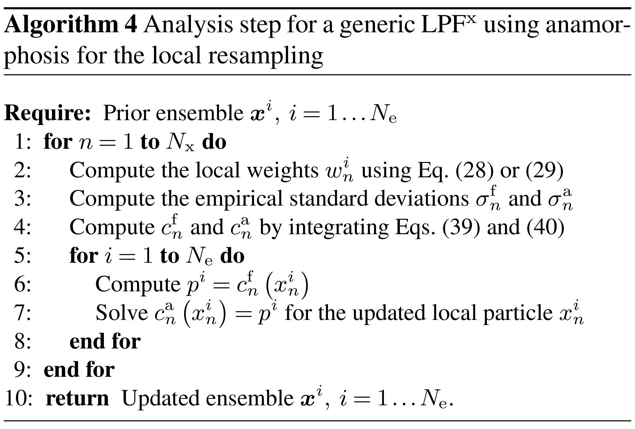
The local resampling algorithm using anamorphosis is, as well as the algorithm using optimal ensemble coupling, a deterministic transformation. This means that unphysical discontinuities due to different random realisations over the grid points are avoided. As explained by Poterjoy (2016), in such an algorithm the updated ensemble members have the same quantiles as the prior ensemble members. The quantile property should, to some extent, be regular in space – for example if the spatial discretisation is fine enough – and this kind of regularity is transferred in the updated ensemble.
When defining the prior and the corrected densities with Eqs. (39) and (40), we introduce some regularisation whose magnitude is controlled through the bandwidth parameter h. Regularisation is necessary to obtain continuous probability density functions. Yet it introduces an additional bias in the analysis step. Typical values of h should be around 1, with larger ensemble sizes Ne requiring smaller values for h. More generally, regularisation is widely used in PF algorithms as a fix to avoid (or at least limit the impact of) weight degeneracy, though its implementation (see Sect. 5.2) is usually different from the method used in this section.
The refinements of the resampling algorithms suggested in Sect. 4.4.2 were designed to minimise the number of unphysical discontinuities in the local resampling step. The goal of the smoothing-by-weights step is to mitigate potential unphysical discontinuities after they have been introduced. On the other hand, the local resampling algorithms based on OT are designed to mitigate the unphysical discontinuities themselves. The main difference between the algorithm based on optimal ensemble coupling and the one based on anamorphosis is that the first one is formulated in the ensemble space, whereas the second one is formulated in the state space. That is to say, in the first case, we build an ensemble transformation Tb, whereas in the second case we build a state transformation Tn.
Due to computational considerations, the optimisation problem Eq. (36) was only considered in one dimension. Hence, contrary to the local resampling algorithm based on optimal ensemble coupling, the one based on anamorphosis is purely one-dimensional and can only be used with blocks of size 1 grid point.
The design of the resampling algorithm based on anamorphosis has been inspired from the kernel density distribution mapping (KDDM) step of the LPF algorithm of Poterjoy (2016), which will be introduced in Sect. 7.3. However, the use of OT has different purposes. In our algorithm, we use the anamorphosis transformation to sample particles from the analysis density, whereas the KDDM step of Poterjoy (2016) is designed to correct the posterior particles – they have already been transformed – with consistent high-order statistical moments.
4.5 Summary for the LPFx algorithms
4.5.1 Highlights
In this section, we have constructed a generic SBD localisation framework, which we have used to define the LPFxs, our first category of LPF methods. The LPFx algorithms are characterised by the geometry of the blocks and domains (i.e. the definition of the local weights) and the resampling algorithm. As shown by Rebeschini and van Handel (2015), the LPFx algorithms have potential to beat the curse of dimensionality. However, unphysical discontinuities are likely to arise after the assembling of locally resampled particles (van Leeuwen, 2009). In this section, we have proposed to mitigate these discontinuities by improving the design of the local resampling step. We distinguished four approaches:
-
A smoothing-by-weights step can be applied after the local resampling step in order to reduce potential unphysical discontinuities. Our method is a generalisation of the original smoothing designed by Penny and Miyoshi (2016) that includes spatial tapering, a smoothing strength, and is suited to the use of state blocks.
-
Simple properties of the local resampling algorithms can be used in order to minimise the occurrences of unphysical discontinuity as shown by Robert and Künsch (2017).
-
Using the principles of discrete OT, we have proposed a resampling algorithm based on a local version of the ETPF of Reich (2013). This algorithm is similar to the PF part of the PF–EnKF hybrid derived by Chustagulprom et al. (2016), but it includes a more general transport cost, and it is suited to the use of blocks and any resampling algorithm. By construction, the distance between the prior and the analysis local ensembles is minimised.
-
By combining the continuous OT problem with the KDE theory, we have derived a new local resampling algorithm based on anamorphosis. We have shown how it helps mitigate the unphysical discontinuities.
In Sect. 4.5.2, we discuss the numerical complexity, and in Sect. 4.5.4, we discuss the asymptotic limits of the proposed LPFx algorithms. In Sect. 4.5.3, we propose guidelines that should inform our choice of the key parameters when implementing these algorithms.
4.5.2 Numerical complexity
We define the auxiliary quantities , , and by
is the maximum number of observation sites in a local domain of radius R. and are the corresponding quantities for the neighbourhood grid points and blocks. In a d-dimensional spatial space, these quantities are at most proportional to Rd.
The complexity of the LPFx analysis is the sum of the complexity of computing all local weights and the complexity of the resampling. Using Eq. (28) or (29), we conclude that the complexity of computing the local weights is , which depends on the localisation radius r and on the complexity Tℋ of applying the observation operator ℋ to a vector. In the following paragraphs we detail the complexity of each resampling algorithm.
When using the multinomial resampling of the SU sampling algorithm for the local resampling, the total complexity of the resampling step is 𝒪(NxNe).
When using optimal ensemble coupling, the resampling step is computationally more expensive, because it requires to solve one optimisation problem for each block. The minimisation coefficients Eq. (35) are computed with complexity , which depends on the distance radius rd. The discrete OT problem Eq. (33) is a particular case of the minimum-cost flow problem and can be solved quite efficiently using the algorithm of Pele and Werman (2009) with complexity . Applying the transformation to the block has complexity . Finally, the total complexity of the resampling step is .
When using optimal transport in state space, every one-dimensional anamorphosis is computed with complexity 𝒪(Np), where Np is the one-dimensional resolution for each state variable. Therefore the total complexity of the resampling step is 𝒪(NxNeNp).
When using the smoothing-by-weights step with the multinomial resampling or the SU sampling algorithm, the smoothed ensemble Eq. (31) is computed with complexity , which depends on the smoothing radius rs, and the updated ensemble Eq. (32) is computed with complexity 𝒪(NxNe). Therefore, the total complexity of the resampling and the smoothing steps is .
For comparison, the more costly operation in the local analysis of a local EnKF algorithm is to compute the singular value decomposition of a matrix, which has complexity assuming that . The total complexity for a local EnKF algorithm depends on the specific implementation but should be at least .
In this complexity analysis, the influence of the parameters r, rd and rs is explicitly shown, because a practitioner must be aware of the numerical cost of increasing these parameters. Since the resampling is performed independently for each block, this algorithmic step (which is the most costly step in practice) can be carried out in parallel, allowing a theoretical gain up to a factor Nb.
4.5.3 Choice of key parameters
The localisation radius r controls the number of observation sites in the local domains and the impact of the curse of dimensionality. To avoid immediate weight degeneracy, r should therefore be relatively small – smaller than what would be required for an EnKF using domain localisation, for example. This is especially true for realistic models with two or more spatial dimensions in which grows as r2 or more. In this case, it can happen that the localisation radius r have to be too small for the method to follow the truth trajectory (either because too much information is ignored, or because there is too much spatial variation in the local weights), which would mean that localisation alone would not be enough to make PF methods operational.
For a local EnKF algorithm, gathering grid points into blocks is an approximation that reduces the numerical cost of the analysis steps by reducing the number of local analyses to perform. For an LPFx algorithm, the local analyses should generally be faster (see the complexity analysis in Sect. 4.5.2). In this case, using larger blocks is a way to decrease the proportion of block borders, which are potential spots for unphysical discontinuities. However, increasing the size of the blocks reduces the number of degrees of freedom to counteract the curse of dimensionality. It also introduces an additional bias in the local weight update, Eq. (28) or (29), since the local weights are computed relatively to the block centres. This issue was identified by Rebeschini and van Handel (2015) as a source of spatial inhomogeneity of the error. For these reasons, the blocks should be small (no more than a few grid points). Only large ensembles could potentially benefit from larger blocks.
More discussion regarding the choice of the localisation radius r and the number of blocks Nb, but also regarding the choice of other parameters (the smoothing radius rs, the smoothing strength αs, the distance radius rd, and the regularisation bandwidth h) can be found in Sect. 5.
4.5.4 Asymptotic limit
An essential property of PF algorithms is that they are asymptotically Bayesian: as stated in Sect. 2.2, under reasonable assumptions, the empirical analysis density converges to the true analysis density for the weak topology on the set of probability measures over in the limit Ne→∞. In this section, we study under which conditions the LPFx analysis can be equivalent to a (global) PF analysis and can therefore be asymptotically Bayesian.
In the limit of very large localisation radius, r→∞, the local weights Eqs. (28) and (29) are equal to the (global) weights of the (global) PF. However, this does not imply that the LPFx analysis is equivalent to a PF analysis, because the resampling is performed independently for each block. Yet we can distinguish the following cases in the limit r→∞:
-
When using independent multinomial resampling or SU sampling for the local resampling, if one uses the same random number for all blocks (this property is always true if Nb=1), then the LPFx analysis is equivalent to the analysis of the PF.
-
When using the smoothing-by-weights step with the multinomial resampling or the SU sampling, if one uses the same random number for all blocks, then the smoothed ensemble Eq. (31) is equal to the (locally) resampled ensemble and the smoothing has no effect: we are back to the first case.
-
When using optimal ensemble coupling for the local resampling, in the limit rd→∞, the LPFx analysis is equivalent to the analysis of the (global) ETPF.
For other cases, we cannot give a firm conclusion:
-
When using independent multinomial resampling or SU sampling for the local resampling with different random number for all blocks, then the updated particles are distributed according to the product of the marginal analysis density Eq. (26), which is, in general, different from the analysis density, even in the limit r→∞.
-
For the same reason, when using anamorphosis for the local resampling, we could not find proof that the LPFx analysis is asymptotically Bayesian, even in the limit h→0 and r→∞.
-
When using the smoothing-by-weights step with the multinomial resampling or the SU sampling, in the limit r→∞ and rs→∞, the smoothed ensemble Eq. (31) can be different from the updated ensemble of the global PF, because the resampling is performed independently for each block.
5.1 Model specifications
In this section, we illustrate the performance of LPFxs with twin simulations of the L96 model in the standard (mildly nonlinear) configuration described in Appendix A3. For this series of experiments, as for all experiments in this paper, the synthetic truth is computed without model error. This is usually a stringent constraint for the PF methods for which accounting for model error is a means for regularisation. But on the other hand, it allows for a fair comparison with the EnKF, and it avoids the issue of defining a realistic model noise.
The distance between the truth and the analysis is measured with the average analysis root mean square error, hereafter simply called the RMSE. To ensure the convergence of the statistical indicators, the runs are at least 5×10⁴Δt long, with an additional 103Δt spin-up period. An advantage of using PF methods is that they should asymptotically yield sharp though reliable ensembles. This may not be entirely reflected in the RMSE. However, not only does the RMSE offer a clear ranking of the algorithms, but it is also an indicator that measures the adequacy to the primary goal of data assimilation, i.e. mean state estimation. Moreover, for a sufficiently cycled DA problem, it seems likely that good RMSE scores can only be achieved with ensembles of good quality in the light of most other indicators. Nonetheless, in addition to the RMSE, rank histograms meant to assess the quality of the ensembles are computed and reported in Appendix D for a selection of experiments.
For the localisation, we assume that the grid points are positioned on an axis with a regular spacing of 1 unit of length and with periodic boundary conditions consistent with the system size. Therefore, the local domain centred on the nth grid point is composed of the points , where ⌊r⌋ is the integer part of the localisation radius and the Nb blocks consist of Nx∕Nb consecutive grid points.
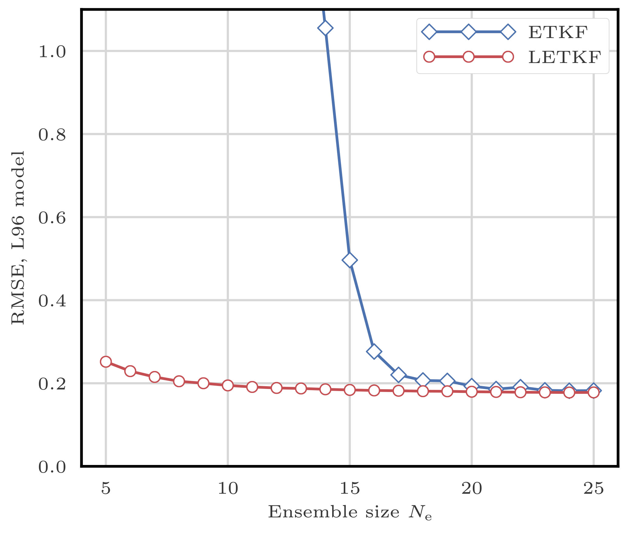
This filtering problem has been widely used to asses the performance of DA algorithms. In this configuration, nonlinearities in the model are rather mild and representative of synoptic scale meteorology, and the error distributions are close to Gaussian. As a reference, the evolution of the RMSE as a function of the ensemble size Ne is shown in Fig. 4 for the ensemble transform Kalman filter (ETKF) and its local version (LETKF). For each value of Ne, the multiplicative inflation parameter and the localisation radius (for the LETKF) are optimally tuned to yield the lowest RMSE. In most of the following figures related to the L96 test series, we draw a baseline at 0.2, roughly the RMSE of the LETKF with Ne=10 particles. Note that slightly lower RMSE scores can be achieved with larger ensembles.
5.2 Perfect model and regularisation
The application of PF algorithms to this chaotic model without error leads to a fast collapse. Even with stochastic models that account for some model error, PF algorithms experience weight degeneracy when the model noise is too low. Therefore, PF practitioners commonly include some additional jitter to mitigate the collapse (e.g. Pham, 2001). As described by Musso et al. (2001), jitter can be added in two different ways.
5.2.1 Pre-regularisation
First, the prediction and sampling step Eq. (7) can be performed using a stochastic extension of the model:
where ℳ is the model associated to the integration scheme of the ordinary differential equations (ODEs), 𝒩(v, Σ) is the normal distribution with mean v and covariance matrix Σ, and q is a tunable parameter. This jitter is meant to compensate for the deterministic nature of the given model. In this case, the truth could be seen as a trajectory of the perturbed model Eq. (44) with a realisation of the noise that is identically zero. In the literature, this method is called pre-regularisation (Le Gland et al., 1998), because the jitter is added before the correction step.
5.2.2 Post-regularisation
Second, a regularisation step can be added after a full analysis cycle:
where s is a tunable parameter. As opposed to the first method, it can be seen as a jitter before integration: the noise is integrated by the model before the next analysis step, while smoothing potential unphysical discontinuities. In some ways this method is similar to additive inflation in EnKF algorithms. It is called post-regularisation (Musso and Oudjane, 1998; Oudjane and Musso, 1999), because the jitter is added after the correction step.
5.2.3 Numerical complexity and asymptotic limit
Both regularisation steps have numerical complexity 𝒪(NxNeTr), with Tr being the complexity of drawing one random number according to the univariate standard normal law 𝒩(0, 1).
The exact LPF is recovered in the limit q→0 and s→0.
5.2.4 Standard S(IR)xR algorithm
With optimally tuned jitter for the standard L96 model, the bootstrap PF algorithm requires about 200 particles to give, on average, more information than the observations.2 With 103 particles, its RMSE is around 0.6, and with 104, it is around 0.4.
We define the standard S(IR)xR algorithm – sampling, importance, resampling, regularisation, the x exponent meaning that steps in parentheses are performed locally for each block – as the LPFx (Algorithm 1) with the following characteristics:
-
Grid points are gathered into Nb blocks of Nx∕Nb connected grid points.
-
Jitter is added after the integration using Eq. (44), with a standard deviation controlled by q.
-
The local weights are computed using the Gaussian tapering of observation influence given by Eq. (29), where G is the Gaspari–Cohn function.
-
The local resampling is performed independently for each block with the adjustment-minimising SU sampling algorithm.
-
Jitter is added at the end of each assimilation cycle using Eq. (45) with a standard deviation controlled by s.
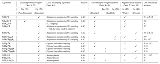
The standard deviation of the jitter after integration (q) and before integration (s) shall be called “integration jitter” and “regularisation jitter”, respectively. The S(IR)xR algorithm has five parameters: . All algorithms tested in this section are variants of this standard algorithm and are named S(αβ)xγδ, with the conventions detailed in Table 1. Table 2 lists all LPFx algorithms tested in this section and reports their characteristics according to the convention of Table 1.
5.3 Tuning the localisation radius
We first check that, in this standard configuration, localisation is working by testing the S(IR)xR algorithm with Nb=40 blocks of size 1 grid point. We take Ne=10 particles, q=0 (perfect model), and several values for the regularisation jitter s. The evolution of the RMSE as a function of the localisation radius r is shown in Fig. 5. With SBD localisation, the LPF yields an RMSE around 0.45 in a regime where the bootstrap PF algorithm is degenerate. The compromise between bias (small values of r, too much information is ignored, or there is too much spatial variation in the local weights) and variance (large values of r, the weights are degenerate) reaches an optimum around r=3 grid points. As expected, the local domains are quite small (5 observation sites) in order to efficiently counteract the curse of dimensionality.
Table 1Nomenclature conventions for the S(αβ)xγδ algorithms. Capital letters refer to the main algorithmic ingredients: “I” for importance, “R” for resampling or regularisation, “T” for transport, and “S” for smoothing. Subscripts are used to distinguish the methods in two different ways. Lower-case subscripts refer to explicit concepts used in the method: “ng” stands for non-Gaussian, “su” for stochastic universal, “s” for state space, and “c” for colour. Upper-case subscripts refer to the work that inspired the method; “PM” stands for Penny and Miyoshi (2016) and “R” for Reich (2013). For simplicity, some subscripts are omitted: “g” for Gaussian, “amsu” for adjustment-minimising stochastic universal, and “w” for white. Finally, note that we used the subscript “d” (for deterministic) to indicate that the same random numbers are used for the resampling over all blocks.
Table 2List of all LPFx algorithms tested in this article. For each algorithm, the main characteristics are reported with appropriate references. The last column indicate the section in which benchmarks based on the L96 model can be found.
5.4 Tuning the jitter
To evaluate the efficiency of the jitter, we experiment with the S(IR)xR algorithm with Ne=10 particles, Nb=40 blocks of size 1 grid point, and a localisation radius r=3 grid points. The evolution of the RMSE as a function of the integration jitter q is shown in Fig. 6 and as a function of the regularisation jitter s in Fig. 7.

Figure 5RMSE as a function of the localisation radius r for the S(IR)xR algorithm with Ne=10 particles, Nb=40 blocks of size 1 grid point, and no integration jitter (q=0). For each r, several values for the regularisation jitter s are tested, as shown by the colour scale.
From these results, we can identify two regimes:
-
With low regularisation jitter (s<0.15), the filter stability is ensured by the integration jitter, with optimal values around q=1.25.
-
With low integration jitter (q<0.5), the stability is ensured by the regularisation jitter, with optimal values around s=0.26.
As expected, adding jitter before integration (i.e. with s) yields significantly better results. This indicates that the model integration indeed smoothes the jitter out and removes unphysical discontinuities for the correction step. We observed the same tendency for most LPFs tested in this article.
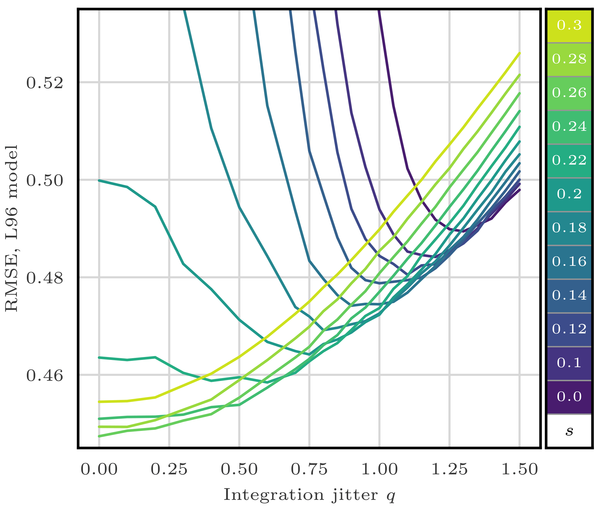
Figure 6RMSE as a function of the integration jitter q for the S(IR)xR algorithm with Ne=10 particles, Nb=40 blocks of size 1 grid point, and a localisation radius r=3 grid points. For each q, several values for the regularisation jitter s are tested, as shown by the colour scale.
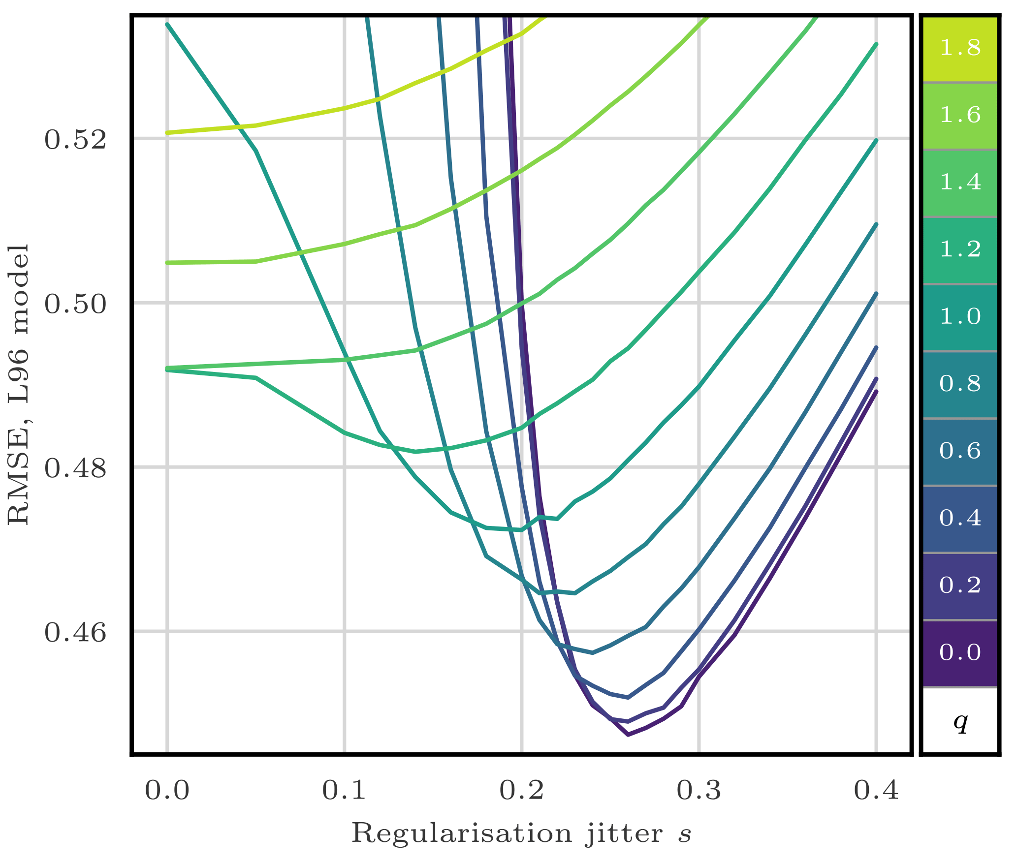
Figure 7RMSE as a function of the regularisation jitter s for the S(IR)xR algorithm with Ne=10 particles, Nb=40 blocks of size 1 grid point, and a localisation radius r=3 grid points. For each s, several values for the integration jitter q are tested, as shown by the colour scale.
In the rest of this section, we take zero integration jitter (q=0), and the localisation radius r and the regularisation jitter s are systematically tuned to yield the lowest RMSE score.
5.5 Increasing the size of the blocks
To illustrate the influence of the size of the blocks, we compare the RMSEs obtained by the S(IR)xR algorithm with various fixed number of blocks Nb. The evolution of the RMSE as a function of the ensemble size Ne is shown in Fig. 8. For small ensemble sizes, using larger blocks is inefficient, because of the need for degrees of freedom to counteract the curse of dimensionality. Only very large ensembles benefit from using large blocks as a consequence of the reduction of proportion of block boundaries, potential spots for unphysical discontinuities.
From now on, unless specified otherwise, we systematically test our algorithms with Nb=40, 20, and 10 blocks of 1, 2, and 4 grid points, respectively, and we keep the best RMSE score.
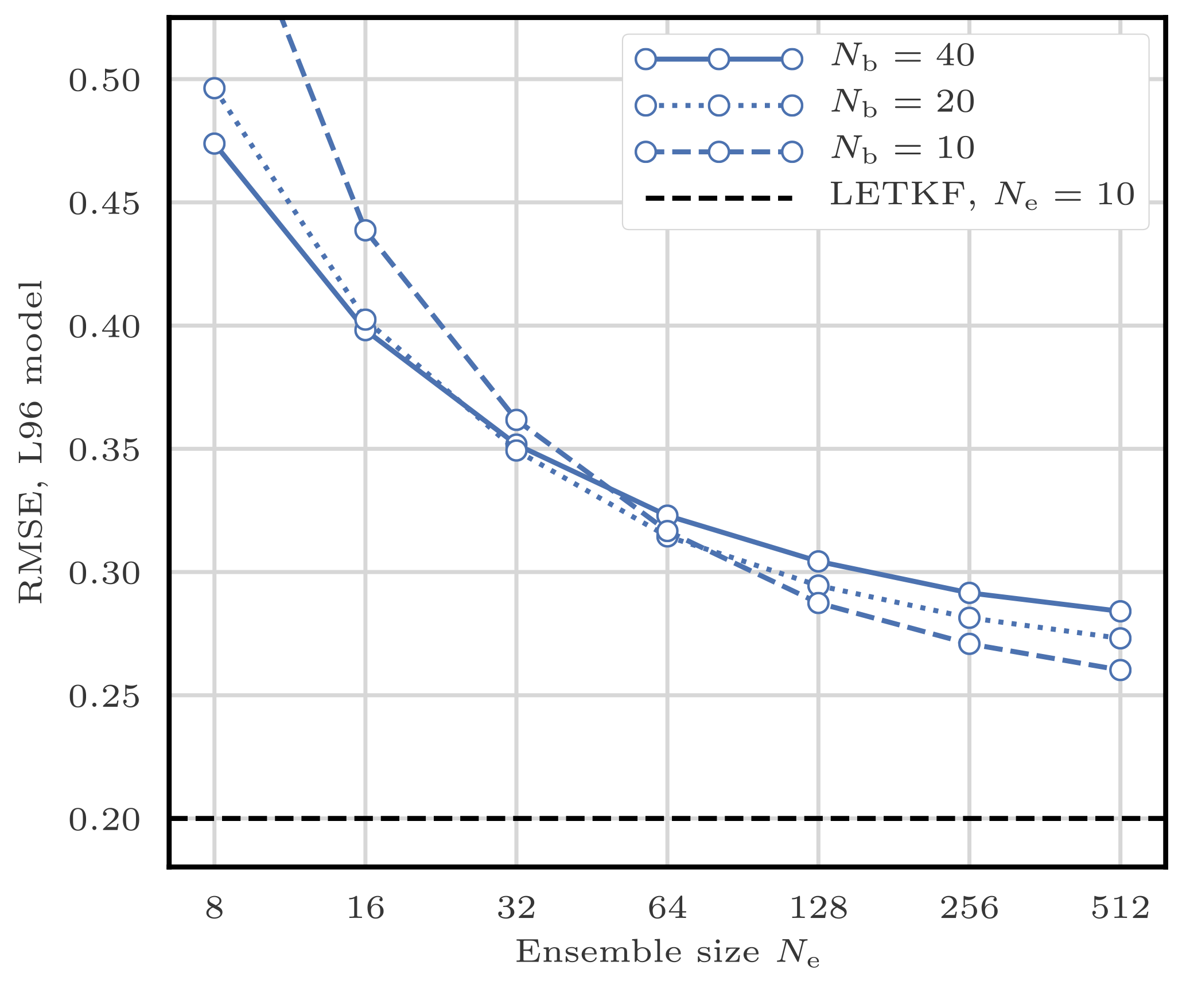
Figure 8RMSE as a function of the ensemble size Ne for the S(IR)xR algorithm with Nb=40, 20, and 10 blocks of size 1, 2, and 4 grid points, respectively.
5.6 Choice of the local weights
To illustrate the influence of the definition of the local weights, we compare the RMSEs of the S(IR)xR and the S(IngR)xR algorithms. These two variants only differ in their definition of the local importance weights: the S(IR)xR algorithm uses the Gaussian tapering of observation influence defined by Eq. (29), while the S(IngR)xR algorithm uses the non-Gaussian tapering given by Eq. (28).
Figure 9 shows the evolution of the RMSE as a function of the ensemble size Ne. The Gaussian version of the definition of the weights always yields better results. This is probably a consequence of the fact that, in this configuration, nonlinearities are mild and the error distributions are close to Gaussian. In the following, we always use Eq. (29) to define the local weights.
5.7 Refining the stochastic universal sampling
In this section, we test the refinements of the sampling algorithms proposed in Sect. 4.4.2. To do this, we compare the S(IR)xR algorithm with the following algorithms:
-
the S(IRd)xR algorithm, for which the same random numbers are used for the resampling of each block;
-
the S(IRsu)xR algorithm, which uses the SU sampling algorithm without the adjustment-minimising property.
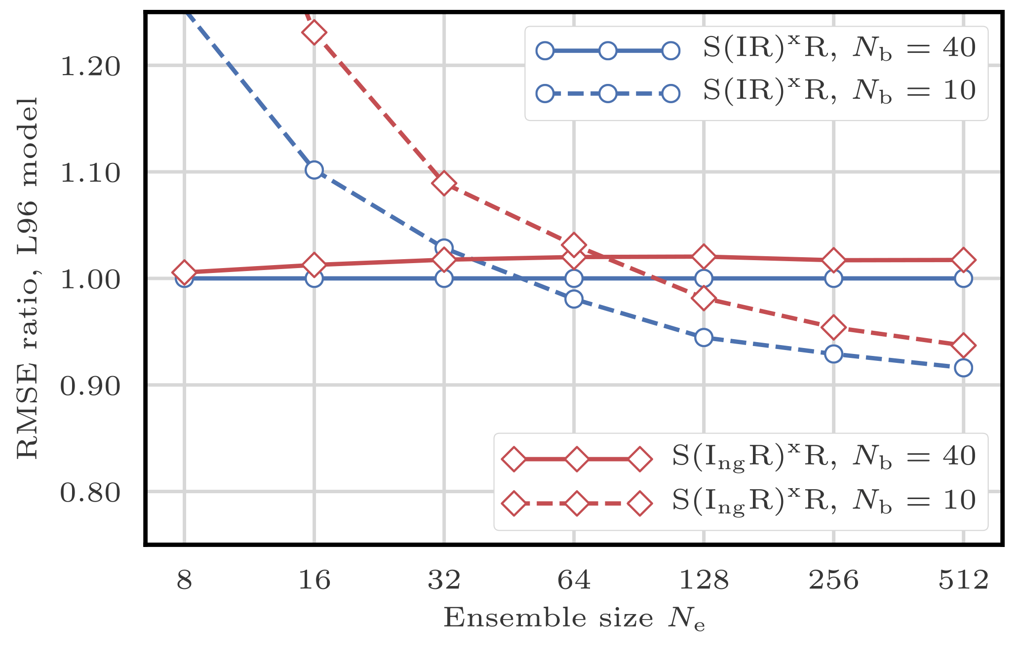
Figure 9RMSE as a function of the ensemble size Ne for the S(IR)xR and the S(IngR)xR algorithms with Nb=40 and 10 blocks of size 1 and 4 grid points, respectively. The scores are displayed in units of the RMSE of the S(IR)xR algorithm with Nb=40 blocks of size 1 grid point.
Figure 10 shows the evolution of the RMSE as a function of the ensemble size Ne. The S(IRsu)xR, the only algorithm that does not satisfy the adjustment-minimising property, yields higher RMSEs. This shows that the adjustment-minimising property is indeed an efficient way of reducing the number of unphysical discontinuities introduced during the resampling step.
However, using the same random number for the resampling of each block does not produce significantly lower RMSEs. This method is insufficient to reduce the number of unphysical discontinuities introduced when assembling the locally updated particles. This is probably a consequence of the fact that the SU sampling algorithm only uses one random number to compute the resampling map. It also suggests that the specific realisation of this random number has a weak influence on long-term statistical properties.
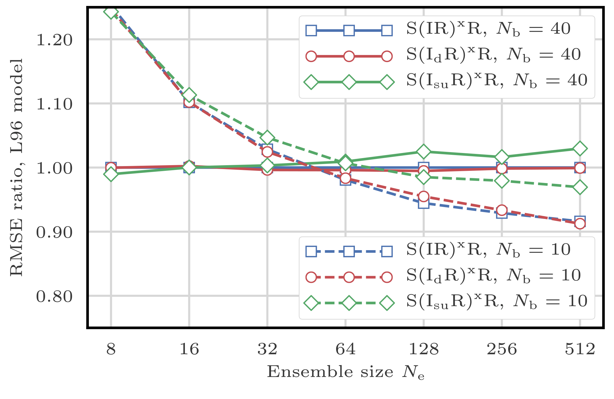
Figure 10RMSE as a function of the ensemble size Ne for the S(IR)xR, the S(IRd)xR, and the S(IRsu)xR algorithms, with Nb=40 and 10 blocks of size 1 and 4 grid points, respectively. The scores are displayed in units of the RMSE of the S(IR)xR algorithm with Nb=40 blocks of size 1 grid point.
In the following, when using the SU sampling algorithm, we always choose its adjustment-minimising form, but we do not enforce the same random numbers over different blocks.
5.8 Colourising the regularisation
5.8.1 Colourisation for global PFs
According to Eqs. (44) and (45), the regularisation jitters are white noises. In realistic models, different state variables may take their values in disjoint intervals (e.g. the temperature takes values around 300 K and the wind speed can take its values between −10 and 10 m s−1), which makes these jittering methods inadequate.
It is hence a common procedure in ensemble DA to scale the regularisation jitter with statistical properties of the ensemble. In a (global) PF context, practitioners often “colourise” the Gaussian regularisation jitter with the empirical covariances of the ensemble as described by Musso et al. (2001). Since the regularisation jitter is added after the resampling step, it is scaled with the weighted ensemble before resampling in order to mitigate the effect of resampling noise.
More precisely, the regularisation jitter has zero mean and Nx×Nx covariance matrix given by
where is the bandwidth, a free parameter, and is the ensemble mean for the nth state variable:
In practice, the Nx×Ne anomaly matrix X is defined by
and the regularisation is added as
where E is the ensemble matrix and Z is a Ne×Ne random matrix whose coefficients are distributed according to a normal law, such that XZ is a sample from the Gaussian distribution with zero mean and covariance matrix Σ. In this case, the regularisation fits in the LET framework with a random transformation matrix.
Colourisation could be added to the integration jitter as well. However in this case, scaling the noise with the ensemble is less justified than for the regularisation jitter. Indeed, the integration noise is inherent to the perturbed model that is used to evolve each ensemble member independently. Hence PF practitioners often take a time-independent Gaussian integration noise whose covariance matrix does not depend on the ensemble but includes some off-diagonal terms based on the distance between grid points (e.g. Ades and van Leeuwen, 2015). However, as we mentioned in Sect. 5.4, we do not use integration jitter for the rest of this article.
5.8.2 Colourisation for LPFs
The 40 variables of the L96 model in its standard configuration are statistically homogeneous with short-range correlations. This is the main reason of the efficiency of the white noise jitter in the S(IR)xR algorithm and its variants tested so far. We still want to investigate the potential gains of using coloured jitters in LPFxs.
In the analysis step of LPFx algorithms, at each grid point, there is a different set of local weights . Therefore it is not possible to compute the covariance of the regularisation jitter with Eq. (46). We propose two different ways of circumventing this obstacle.
A first approach could be to scale the regularisation with the locally resampled ensemble, since in this case all weights are equal. This is the approach followed by Reich (2013) and Chustagulprom et al. (2016) under the name “particle rejuvenation”. However, this approach systematically leads to higher RMSEs for the S(IR)xR algorithm (not shown here). This can be potentially explained by two factors. First, the resampling could introduce noise in the computation of the anomaly matrix X. Second, the fact that the resampling is performed independently for each block perturbs the propagation of multivariate properties (such as sample covariance) over different blocks.
In a second approach, the anomaly matrix X is defined by the weighted ensemble before resampling, i.e. using the local weights , as follows:
In this case, the Gaussian regularisation jitter has the following covariance matrix:
which is a generalisation of Eq. (46). This method can also be seen as a generalisation of the adaptative inflation used by Penny and Miyoshi (2016). For their adaptative inflation, Penny and Miyoshi (2016) only computed the diagonal of the matrix X and fixed the bandwidth parameter to 1. Our approach yields a lowest RMSE in all tested cases, which is most probably due to the tuning of the bandwidth parameter .
5.8.3 Numerical complexity and asymptotic limit
The coloured regularisation step has complexity . It is slightly more costly than using the white noise regularisation step, due to the matrix product Eq. (49).
The exact LPF is recovered in the limit .
5.8.4 Illustrations
We experiment with the S(IR)xRc algorithm, in which the regularisation jitter is colourised as described by Eqs. (49) and (50). In this algorithm, the parameter s (regularisation jitter standard deviation) is replaced by the bandwidth parameter , hereafter simply called regularisation jitter. The evolution of the RMSE as a function of for the S(IR)xRc algorithm (not shown here) is very similar to the evolution of the RMSE as a function of s for the S(IR)xR algorithm. In the following, when using the coloured regularisation jitter method, is systematically tuned to yield the lowest RMSE score.
Figure 11 shows the evolution of the RMSE as a function of the ensemble size Ne for the S(IR)xR and the S(IR)xRc algorithms. These two variants only differ by the regularisation method. The S(IR)xR algorithm uses white regularisation jitter, while the S(IR)xRc algorithm uses coloured regularisation jitter. For small ensembles, the S(IR)xRc algorithm yields higher RMSEs, whereas it shows slightly better RMSEs for larger ensembles. Depending on the block size, the transition between both regimes happens when the ensemble size Ne is between 32 to 64 particles. The higher RMSEs of the S(IR)xRc algorithm for small ensembles may have two potential explanations. First, even if the L96 model in its standard configuration is characterised by short-range correlations, the covariance matrix Σ is a high-dimensional object that is poorly represented with a weighted ensemble. Second, the analysis distribution for small ensemble may be too different from a Gaussian for the coloured regularisation jitter method to yield better results, even though in this mildly nonlinear configuration, the densities are close to Gaussian.
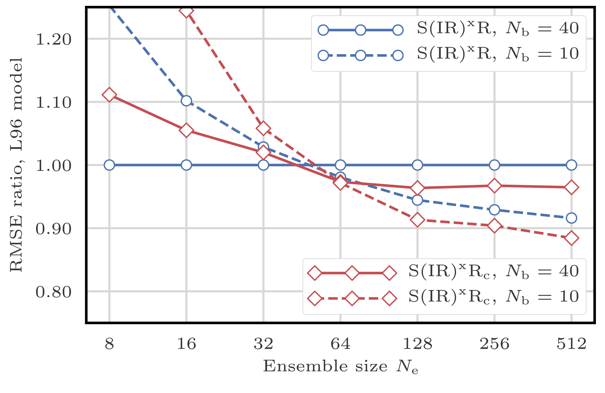
Figure 11RMSE as a function of the ensemble size Ne for the S(IR)xR and the S(IR)xRc algorithms with Nb=40 and 10 blocks of size 1 and 4 grid points, respectively. The scores are displayed in units of the RMSE of the S(IR)xR algorithm with Nb=40 blocks of size 1 grid point.
5.9 Applying a smoothing-by-weights step
In this section, we look for the potential benefits of adding a smoothing-by-weights step as presented in Sect. 4.4.1, by testing the S(IR)xSPMR and the S(IR)xSPMRc algorithms. These algorithms only differ from the S(IR)xR and the S(IR)xRc algorithms by the fact that they add a smoothing-by-weights step as specified in Algorithm 2.
Alongside the smoothing-by-weights step come two additional tuning parameters: the smoothing strength αs and the smoothing radius rs. We first investigate the influence of theses parameters. Figure 12 shows the evolution of the RMSE as a function of the smoothing radius rs for the S(IR)xSPMR with Ne=10 particles and Nb=40 blocks of size 1 grid point for several values of the smoothing strength αs. As before, the localisation radius r and the regularisation jitter s are optimally tuned.
At a fixed smoothing strength αs>0, starting from rs=1 grid point (no smoothing), the RMSE decreases when rs increases. It reaches a minimum and then increases again. In this example, the optimal smoothing radius rs lies between 5 and 6 grid points for a smoothing strength αs=1, with a corresponding optimal localisation radius r between 2 and 3 grid points and optimal regularisation jitter s around 0.45 (not shown here). For comparison, the optimal tuning parameters for the S(IR)xR algorithm in the same configuration were r between 4 and 5 grid points and s around 0.2.
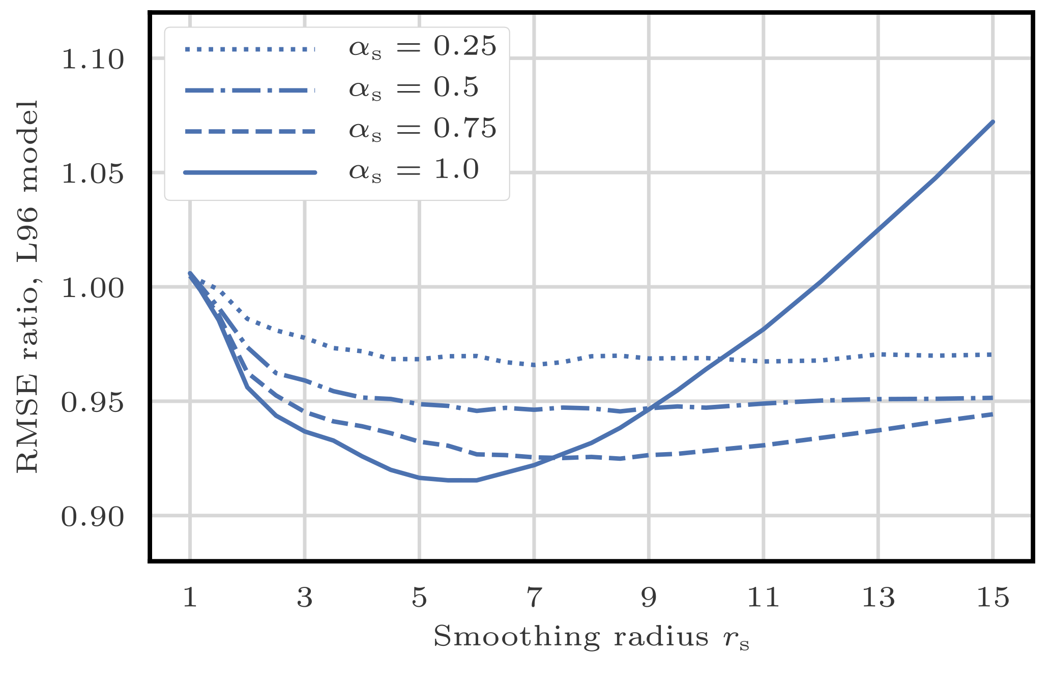
Figure 12RMSE as a function of the smoothing radius rs for the S(IR)xSPMR algorithms with Ne=16 particles and Nb=40 blocks of size 1 grid point for several values of the smoothing strength αs. The scores are displayed in units of the RMSE of the S(IR)xR algorithm with Ne=16 particles and Nb=40 blocks of size 1 grid point.
Based on extensive tests of the S(IR)xSPMR and the S(IR)xSPMRc algorithms with Ne ranging from 8 to 128 particles (not shown here), we draw the following conclusions:
-
In general αs=1 is optimal, or at least only slightly suboptimal.
-
Optimal values for r and s are larger with the smoothing-by-weights step than without it.
-
Optimal values for r and rs are not related and must be tuned separately.
In the following, when using the smoothing-by-weights method, we take αs=1, and rs is tuned to yield the lowest RMSE score – alongside the tuning of the localisation radius r and the regularisation jitter s or . Figure 13 shows the evolution of the RMSE as a function of the ensemble size Ne for the S(IR)xSPMR and the S(IR)xSPMRc algorithms. The S(IR)xSPMR algorithm yields systematically lower RMSEs than the standard S(IR)xR. However, as the ensemble size Ne grows, the gain in RMSE score becomes very small. With Ne=512 particles, there is almost no difference between both scores. In this case, the optimal smoothing radius rs is around 5 grid points, much smaller than the optimal localisation radius r around 15 grid points, such that the smoothing-by-weights step does not modify the analysis ensemble much. The S(IR)xSPMRc algorithm also yields lower RMSEs than the S(IR)xRc algorithm. Yet, in this case, the gain in RMSE is still significant for large ensembles, and with Ne=512 particles, the RMSEs are even comparable to those of the EnKF.
From these results, we conclude that the smoothing-by-weights step is an efficient way of mitigating the unphysical discontinuities that were introduced when assembling the locally updated particles, especially when combined with the coloured noise regularisation jitter method.

Figure 13RMSE as a function of the ensemble size Ne for S(IR)xR, the S(IR)xRc, the S(IR)xSPMR, and the S(IR)xSPMR algorithms.
5.10 Using optimal transport in ensemble space
In this section, we evaluate the efficiency of using the optimal transport in ensemble space as a way to mitigate the unphysical discontinuities of the local resampling step by experimenting the S(ITR)xR and the S(ITR)xRc algorithms. These algorithms only differ from the S(IR)xR and the S(IR)xRc algorithms by the fact that they use optimal ensemble coupling for the local resampling as described by Algorithm 3.
For each block, the local linear transformation is computed by solving the minimisation problem Eq. (33), which can be seen as a particular case of the minimum-cost flow problem. We choose to compute its numerical solution using the network simplex algorithm implemented by the graph library LEMON (Dezső et al., 2011). As described in Sect. 4.4.3, this method is characterised by an additional tuning parameter: the distance radius rd. We have investigated the influence of the parameters Nb and rd by performing extensive tests of the S(ITR)xR and the S(ITR)xRc algorithms with Ne ranging from 8 to 128 particles (not shown here) and draw the following conclusions.
Optimal values for the distance radius rd are much smaller than the localisation radius and are even smaller than 2 grid points most of the time. Using rd=1 grid point yields RMSEs that are only very slightly suboptimal. Moreover, all other things being equal, using Nb=20 blocks of size 2 grid points systematically yields higher RMSEs than using Nb=40 blocks of size 1 grid point.
In the following, when using the optimal ensemble coupling algorithm, we take rd=1 grid point and Nb=40 blocks of size 1 grid point. Figure 14 shows the evolution of the RMSE as a function of the ensemble size Ne for the S(ITR)xR and the S(ITR)xRc algorithms. Using optimal ensemble coupling for the local resampling step always yields significantly lower RMSEs than using the SU sampling algorithm. Yet in this case, using the coloured noise regularisation jitter method does not improve the RMSEs for very large ensembles.
We have also performed extensive tests with Ne ranging from 8 to 128 particles on the S(ITR)xSPMR and the S(ITR)xSPMRc algorithms in which the optimal ensemble coupling resampling method is combined with the smoothing-by-weights method (not shown here). Our implementations of these algorithms are numerically more costly. For small ensembles (Ne≤32 particles), the RMSEs of the S(ITR)xSPMR and the S(ITR)xSPMRc algorithms are barely smaller than those of the S(ITR)xR and the S(ITR)xRc algorithms. With larger ensembles, we could not find a configuration where using the smoothing-by-weights method yields better RMSEs.
The fact that neither the use of larger blocks nor the smoothing-by-weights step significantly improves the RMSE score when using optimal ensemble coupling indicates that this local resampling method is indeed an efficient way of mitigating the unphysical discontinuities inherent to assembling the locally updated particles.
5.11 Using continuous optimal transport
In this section, we test the efficiency of using the optimal transport in state space as a way to mitigate the unphysical discontinuities of the local resampling step by experimenting the S(ITs)xR and the S(ITs)xRc algorithms. These algorithms only differ from the S(IR)xR and the S(IR)xRc algorithms by the fact that they use anamorphosis for the local resampling, as described by Algorithm 4.
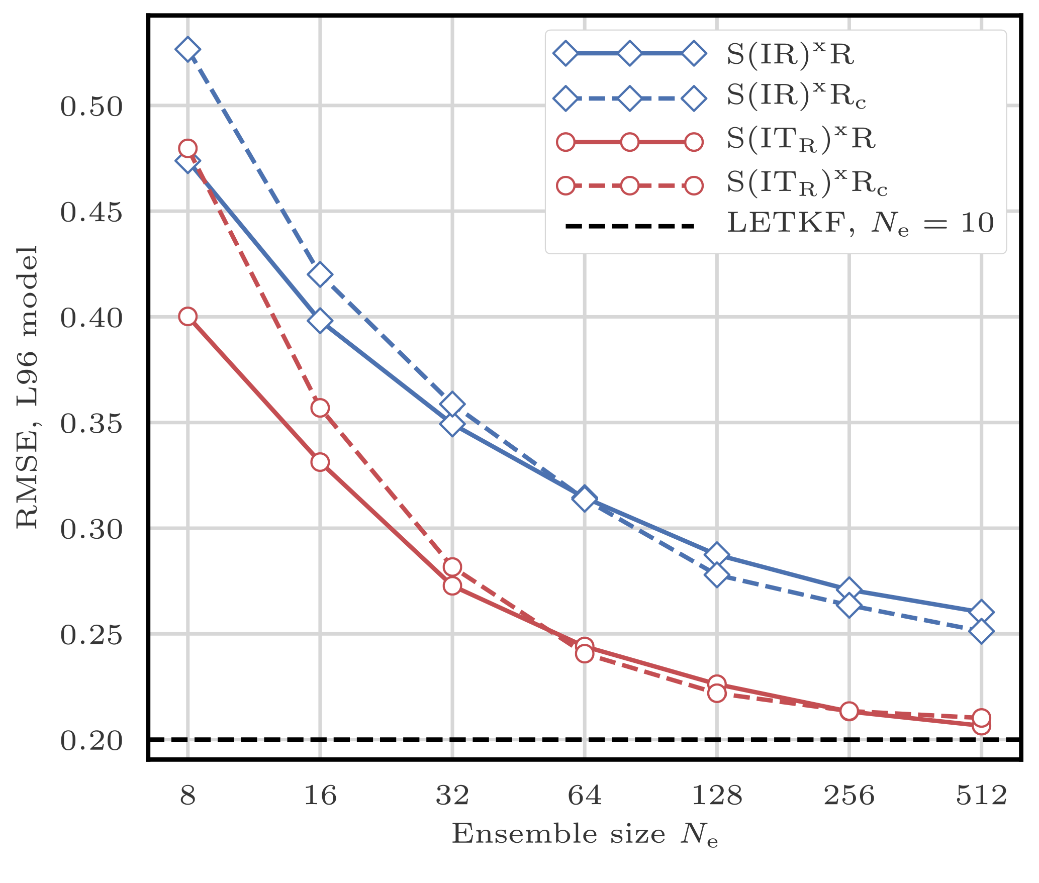
Figure 14RMSE as a function of the ensemble size Ne for the S(IR)xR, the S(IR)xRc, the S(ITR)xR, and the S(ITR)xRc algorithms.
As mentioned in Sect. 4.4.4, the local resampling algorithm based on anamorphosis uses blocks of size 1 grid point. Hence, when using the S(ITs)xR and the S(ITs)xRc algorithms, we take Nb=40 blocks of size 1 grid point. The definition of the state transformation map T is based on the prior and corrected densities given by Eqs. (39) and (40) using the Student's t distribution with two degrees of freedom for the regularisation kernel K. It is characterised by an additional tuning parameter: h, hereafter called regularisation bandwidth – different from the regularisation jitter . We have investigated the influence of the regularisation bandwidth h by performing extensive tests of the S(ITs)xR and the S(ITs)xRc algorithms, with Ne ranging from 8 to 128 particles (not shown here). For small ensembles (Ne≤16 particles), optimal values for h lie between 2 and 3, the RMSE score obtained with h=1 being very slightly suboptimal. For larger ensembles, we did not find any significant difference between h=1 and larger values.
In the following, when using the anamorphosis resampling algorithm, we take the standard value h=1. Figure 15 shows the evolution of the RMSE as a function of the ensemble size Ne for the S(ITs)xR and the S(ITs)xRc algorithms. These algorithms yield RMSEs even lower than the algorithms using optimal ensemble coupling. However in this case, using the coloured noise regularisation jitter method always yields significantly higher RMSEs than using the white noise regularisation method. It is probably a consequence of the fact that some coloured regularisation is already introduced in the nonlinear transformation process through the kernel representation of the densities with Eqs. (39) and (40). It may also be a consequence of the fact that the algorithms using anamorphosis for the local resampling step cannot be written as a local LET algorithm, contrary to the algorithms using the SU sampling or the optimal ensemble coupling algorithms.
We have also performed extensive tests with Ne ranging from 8 to 128 particles on the S(ITs)xSPMR algorithm, in which the anamorphosis resampling method is combined with the smoothing-by-weights method (not shown here). As for the S(ITR)xSPMR and the S(ITR)xSPMRc algorithms, our implementation is significantly numerically more costly, and adding the smoothing-by-weights step only yields minor RMSE improvements.

Figure 15RMSE as a function of the ensemble size Ne for the S(IR)xR, the S(IR)xRc, the S(ITs)xR, and the S(ITs)xRc algorithms.
These latter remarks, alongside significantly lower RMSEs for the S(ITs)xR algorithm than for the S(IR)xR, indicate that the local resampling method based on anamorphosis is, as well as the method based on optimal ensemble coupling, an efficient way of mitigating the unphysical discontinuities inherent to assembling the locally updated particles.
5.12 Summary
To summarise, Fig. 16 shows the evolution of the RMSE as a function of the ensemble size Ne for the main LPFxs tested in this section. For small ensembles (Ne≤32 particles), the algorithms using OT-based resampling methods clearly yield lower RMSEs than the other algorithms. For large ensemble (Ne≥128 particles), combining the smoothing-by-weights method with the coloured noise regularisation jitter methods yields equally good scores as the algorithms using OT. For Ne=512 particles (the largest ensemble size tested with the L96 model), the best RMSE scores obtained with LPFxs become comparable to those of the EnKF.
In this standard, mildly nonlinear configuration where error distributions are close to Gaussian, the EnKF performs very well, and the LPFx algorithms tested in this section do not clearly yield lower RMSE scores than the ETKF and the LETKF. There are several potential reasons for this. First, the ETKF and the LETKF rely on more information than the LPFxs because they use Gaussian error distributions, which is a good approximation in this configuration. Second, the values of the optimal localisation radius r for the LPFxs are, in most cases, smaller than the value of the optimal localisation radius r for the LETKF, because localisation has to counteract the curse of dimensionality. This means that, in this case, localisation introduces more bias in the PF than in the EnKF. Third, using a non-zero regularisation jitter is necessary to avoid the collapse of the LPFxs without model error. This method introduces an additional bias in the LPFx analysis. In practice, we have found, in this case, that the values of the optimal regularisation jitter for the LPFxs are rather large, whereas the optimal inflation factor in the ETKF and the LETKF is small.
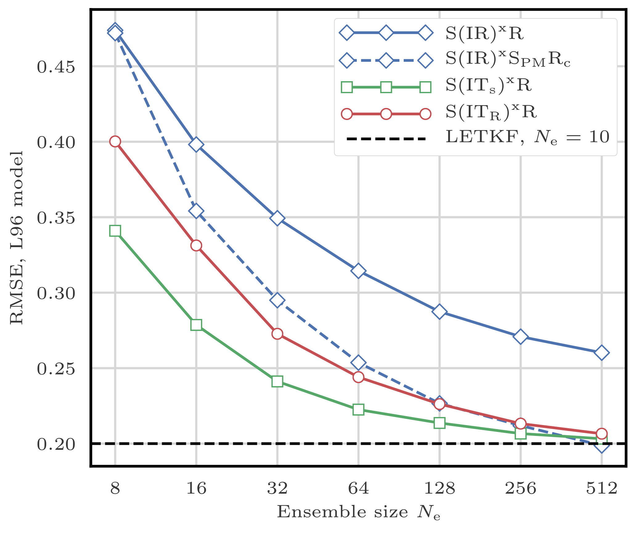
Figure 16RMSE as a function of the ensemble size Ne for the main LPFxs tested in this section.
Note that our objective is not to design LPF algorithms that beat the EnKF in all situations, but rather to incrementally improve the PF. However, specific configurations in which the EnKF fails and the PF succeeds can easily be conceived by increasing nonlinearities. Such a configuration is studied in Appendix C.
As a complement to this RMSE test series, rank histograms for several LPFs are computed, reported, and discussed in Appendix D.
6.1 Model specifications
In this section, we illustrate the performance of LPFxs with twin simulations of the barotropic vorticity (BV) model in the coarse-resolution (CR) configuration described in Appendix A4.1. Using this configuration yields a DA problem of sizes Nx=1024 and Ny=256. As mentioned in Appendix A4.1, the spatial resolution is enough to capture the dynamics of a few vortices, and the model integration is not too expensive, such that we can perform extensive tests with small to moderate ensemble sizes.
As with the L96 model, the distance between the truth and the analysis is measured with the average analysis RMSE. The runs are 9×10³Δt long with an additional 103Δt spin-up period, more than enough to ensure the convergence of the statistical indicators.
For the localisation, we use the underlying physical space with the Euclidean distance. The geometry of the blocks and domain are constructed as described by Fig. 2. Specifically, blocks are rectangles and local domains are disks, with the difference that the doubly periodic boundary conditions are taken into account.
6.2 Scores for the EnKF and the PF
As a reference, we first compute the RMSEs of the EnKF with this model. Figure 17 shows the evolution of the RMSE as a function of the ensemble size Ne for the ETKF and the LETKF. For each value of Ne, the inflation parameter and the localisation radius (only for the LETKF) are optimally tuned to yield the lowest RMSE.
The ETKF requires at least Ne=12 ensemble members to avoid divergence. The best RMSEs are approximately 20 times smaller than the observation standard deviation (σ=0.3). Even with only Ne=8 ensemble members, the LETKF yields RMSEs at least 10 times smaller than the observation standard deviation, showing that, in this case, localisation is working as expected. In this configuration, the observation sites are uniformly distributed over the spatial domain. This constrains the posterior probability density functions to be close to Gaussian, which explains the success of the EnKF in this DA problem.
With Ne≤1024 particles, we could not find a combination of tuning parameters with which the bootstrap filter or the ETPF yield RMSEs significantly lower than 1. In the following figures related to this BV test series, we draw a baseline at σ∕20, which is roughly the RMSE of the ETKF and the LETKF with Ne=12 particles. Note that slightly lower RMSE scores can be achieved with larger ensembles.
6.3 Scores for the LPFx algorithms
In this section, we test the LPFx algorithms with Ne ranging from 8 to 128 particles. The nomenclature for the algorithms is the same as in Sect. 5. In particular, all algorithms tested in this Section are in the list reported in Table 2.
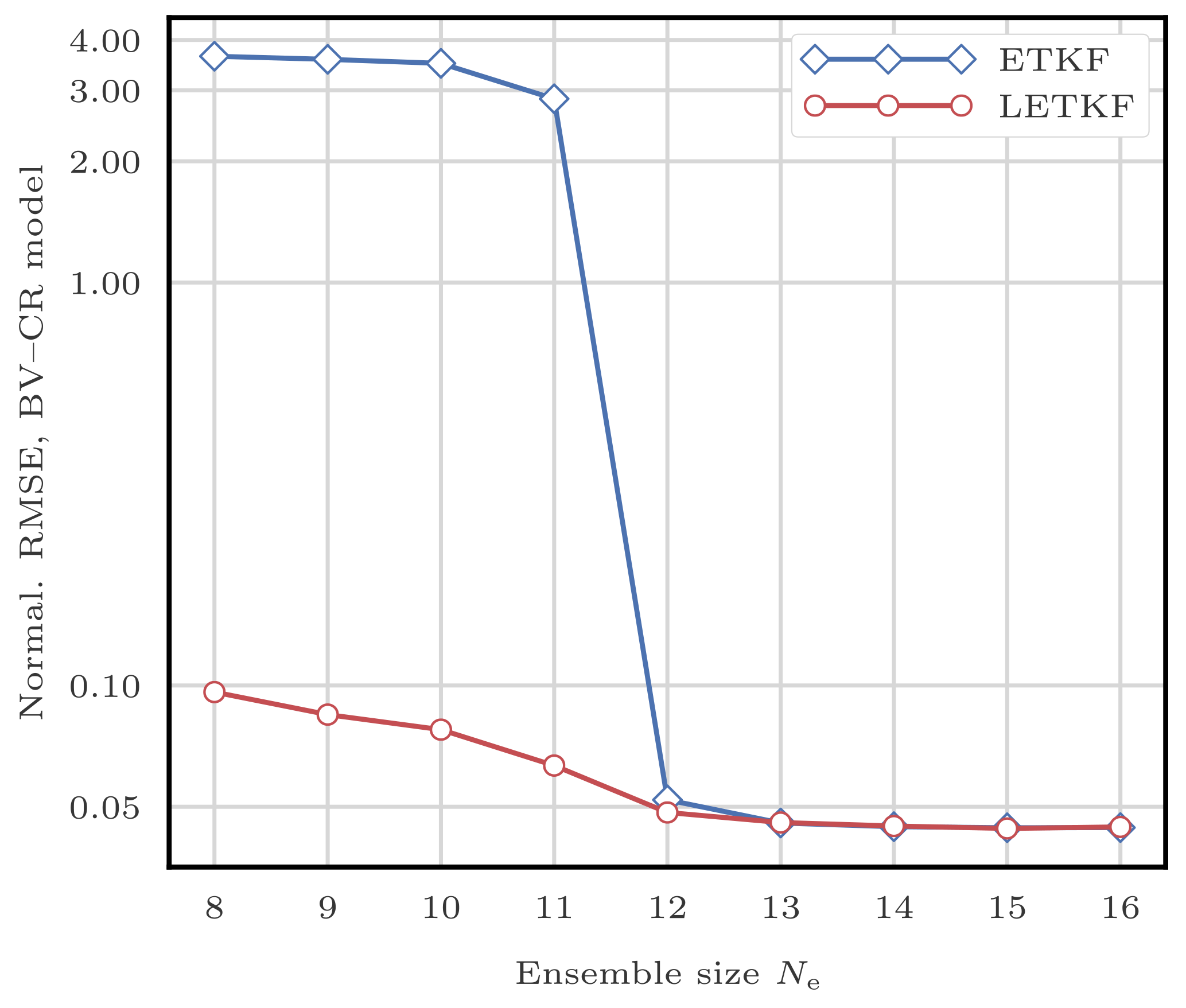
Figure 17RMSE as a function of the ensemble size Ne for the ETKF and the LETKF. The scores are displayed in units of the observation standard deviation σ.
For each ensemble size Ne, the parameter tuning methods are similar to those in the L96 test series and can be described as follows:
-
We take zero integration jitter (q=0).
-
The localisation radius r is systematically tuned to yield the lowest RMSE score.
-
The regularisation jitter s (or when using the coloured noise regularisation jitter method) is systematically tuned as well.
-
For the algorithms using the SU sampling algorithm (i.e. the S(IR) variants), we test four values for the number of blocks Nb, and we keep the best RMSE score:
-
1024 blocks of shape 1×1 grid point,
-
256 blocks of shape 2×2 grid points,
-
64 blocks of shape 4×4 grid points,
-
16 blocks of shape 8×8 grid points.
-
-
For the algorithms using optimal ensemble coupling or anamorphosis (i.e. the S(IT∗)x∗ variants), we only test blocks of shape 1×1 grid point.
-
When using the smoothing-by-weights method, we take the smoothing strength αs=1, and the smoothing radius rs is optimally tuned to yield the lowest RMSE score.
-
When using the optimal ensemble coupling for the local resampling step, the distance radius rd is optimally tuned to yield the lowest RMSE score.
-
When using the anamorphosis for the local resampling step, we take the regularisation bandwidth h=1.
Figure 18 shows the evolution of the RMSE as a function of the ensemble size Ne for the LPFxs. Most of the conclusions related to the L96 model remain true to the BV model. The best RMSE scores are obtained with algorithms using OT-based resampling methods. Combining the smoothing-by-weights method with the coloured noise regularisation jitter methods yields almost equally good scores as the algorithms using OT. Yet some differences can be pointed out.
With such a large model, we expected the coloured noise regularisation jitter method to be much more effective than the white noise method, because the colourisation reduces potential spatial discontinuities in the jitter. We observe indeed that the S(IR)xRc and the S(IR)xSPMRc algorithms yield significantly lower RMSEs than the S(IR)xR and the S(IR)xSPMR algorithms. Yet the S(ITR)xRc and the S(ITs)xRc algorithms are clearly outperformed by both the S(ITR)xR and the S(ITs)xR algorithms in terms of RMSEs. This suggests that there is room for improvement in the design of regularisation jitter methods for PF algorithms.
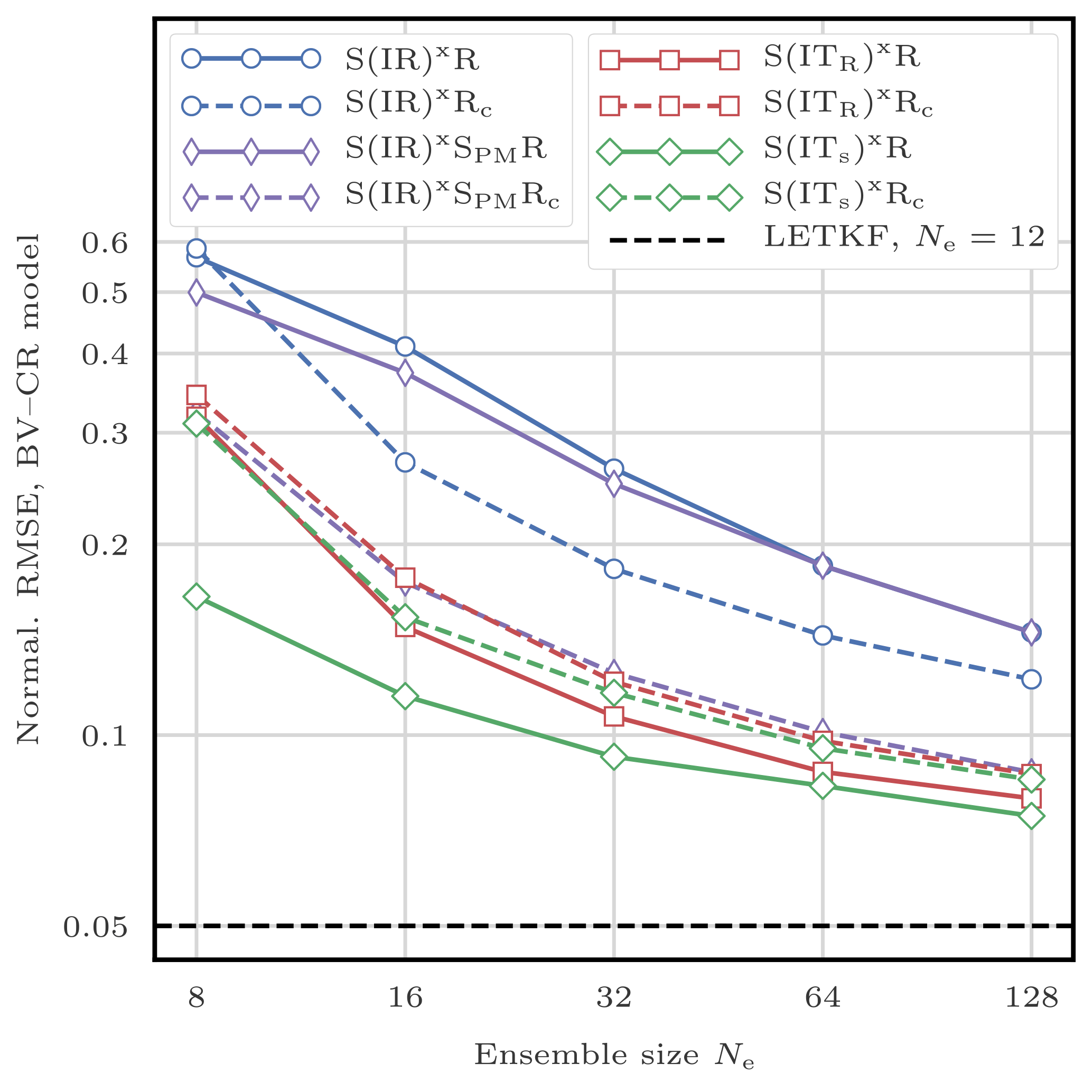
Figure 18RMSE as a function of the ensemble size Ne for the LPFxs. The scores are displayed in units of the observation standard deviation σ.
Due to relatively high computational times, we restricted our study to reasonable ensemble sizes, Ne≤128 particles. In this configuration, the RMSE scores of LPFxs are not yet comparable with those of the EnKF (see Fig. 18).
Finally, it should be noted that for the S(ITR)xR and the S(ITR)xRc algorithms with Ne≥32 particles, optimal values for the distance radius rd lie between 3 and 6 grid points (not shown here), contrary to the results obtained with the L96 model, for which rd=1 grid point could be considered optimal. More generally for all LPFxs, the optimal values for the localisation radius r (not shown here) are significantly larger (in number of grid points) for the BV model than for the L96 model.
In the SBD localisation formalism, each block of grid points is updated using the local domain of observation sites that may influence these grid points. In the sequential–observation (SO) localisation formalism, we use a different approach. Observations are assimilated sequentially, and assimilating the observation at a site should only update nearby grid points. LPF algorithms using the SO localisation formalism will be called LPFy algorithms3.
In this section, we set q∈{1…Ny}, and we describe how to assimilate the observation yq. In Sect. 7.1, we introduce the state space partitioning. The resulting decompositions of the conditional density are discussed in Sect. 7.2. Finally, practical algorithms using these principles are derived in Sect. 7.3 and 7.4.
These algorithms are designed to assimilate one observation at a time. Hence, a full assimilation cycle requires Ny sequential iterations of these algorithms, during which the ensemble is gradually updated: the updated ensemble after assimilating yq will be the prior ensemble to assimilate yq+1.
7.1 Partitioning the state space
Following Robert and Künsch (2017) the state space is divided into three regions:
-
The first region U covers all grid points that directly influence yq: if ℋ is linear, it is all columns of ℋ that have non-zero entries on row q.
-
The second region V gathers all grid points that are deemed correlated to those in U.
-
The third region W contains all remaining grid points.
The meaning of “correlated” is to be understood as a prior hypothesis, where we define a valid tapering matrix C that represents the decay of correlations. Non-zero elements of C should be located near the main diagonal and reflect the intensity of the correlation. A popular choice for C is the one obtained using the Gaspari–Cohn function G:
where dm, n is the distance between the mth and nth grid points and r is the localisation radius, a free parameter similar to the localisation radius defined in the SBD localisation formalism (see Sect. 4.2.2).
The UVW partition of the state space is a generalisation of the original LG partition introduced by Bengtsson et al. (2003), in which U and V are gathered into one region L, the local domain of yq, and W is called G (for global). Figure 19 illustrates this UVW partition. We emphasise that both the LG and the UVW state partitions depend on the site of observation yq. They are fundamentally different from the (local state) block decomposition of Sect. 4.2.1. Therefore they shall simply be called “partition” to avoid confusion.
7.2 The conditional density
For any region A of the physical space, let xA be the restriction of vector x to A, i.e. the state variables of x whose grid points are located within A.
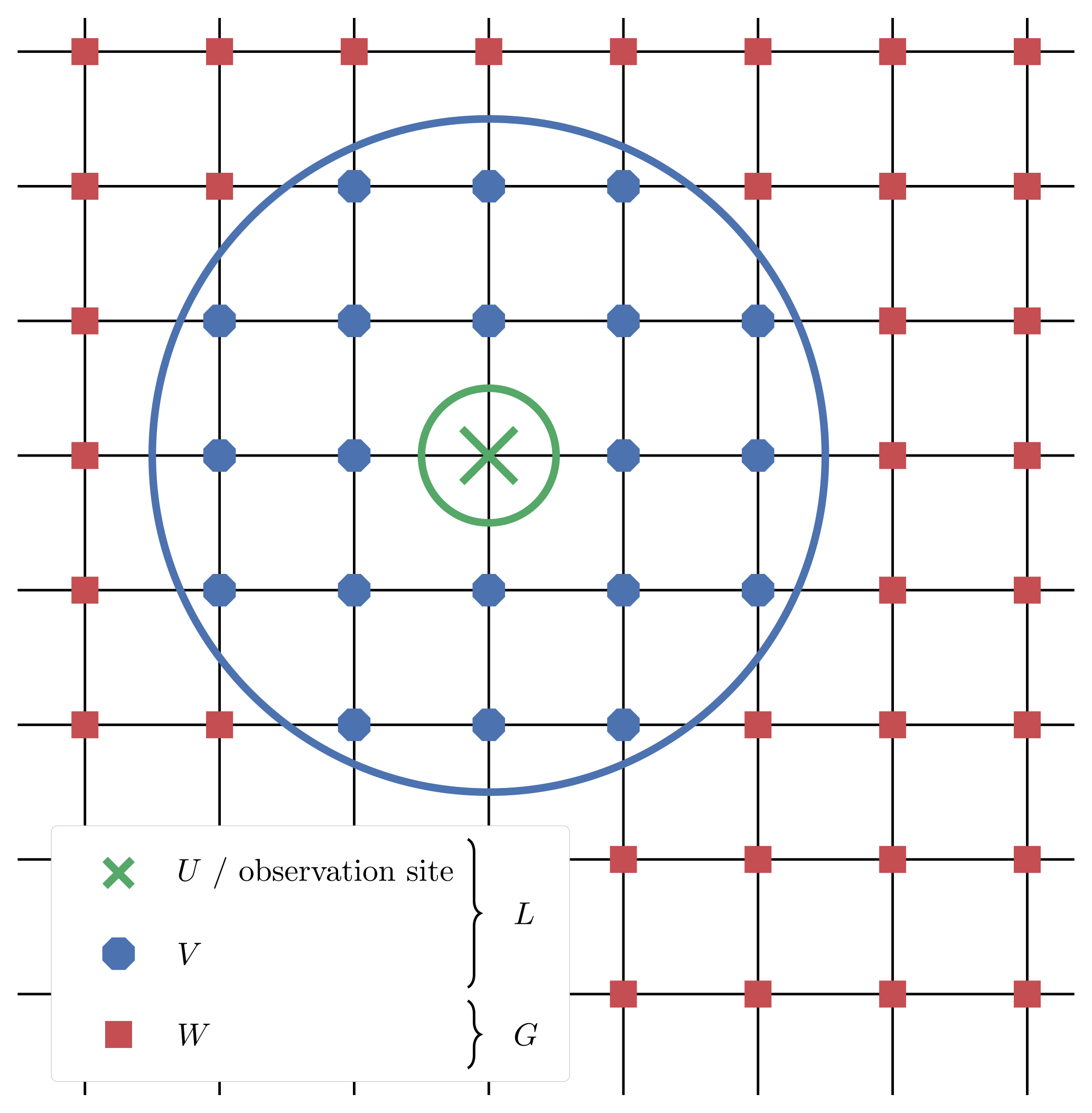
Figure 19Example of the UVW partition for a two-dimensional space. The site of observation yq lies in the middle. The local regions U and V are circumscribed by the thick green and blue circles and contain 1 and 20 grid points, respectively. The global region W contains all remaining grid points. In the case of the LG partition, the local region L gathers all 21 grid points in U and V.
7.2.1 With the LG partition
Without loss of generality, the conditional density is decomposed into
In a localisation context, it seems reasonable to assume that xG and yq are independent, that is
and the conditional pdf of the L region can be written as
This yields an assimilation method for yq described by Algorithm 5.
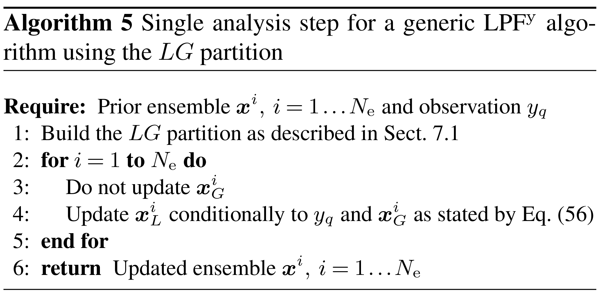
7.2.2 With the UVW partition
With the UVW partition, the conditional density is factored as
If one assumes that the U and W regions are not only uncorrelated but also independent, then one can make the additional factorisation:
Finally, the conditional density is
The assimilation method for yq is now described by Algorithm 6.
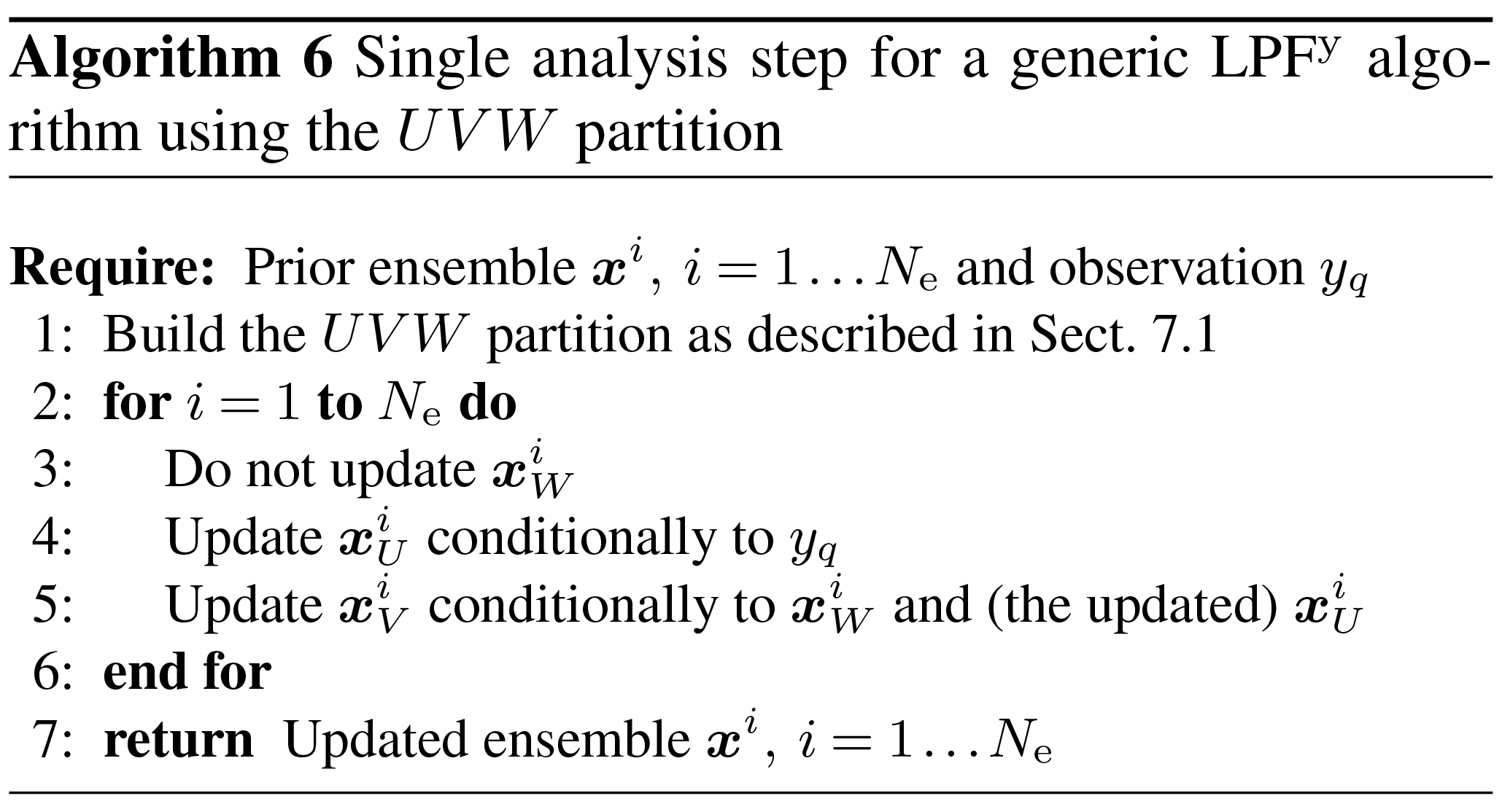
7.2.3 The partition and the particle filter
So far, the SO formalism looks elegant. The resulting assimilation schemes avoid the discontinuity issue inherent to the SBD formalism by using conditional updates of the ensemble.
However, this kind of update seems hopeless in a PF context. Indeed the factors p(xG, xL) and in Eqs. (56) and (60) will be non-zero only if the updated particles are copies of the prior particles, which spoils the entire purpose of localising the assimilation. Hence potential solutions need to make approximations of the conditional density.
7.2.4 The multivariate rank histogram filter
Similar principles were used to design the multivariate rank histogram filter (MRHF) of Metref et al. (2014), with the main difference that the state space is entirely partitioned as follows. Assuming that yq only depends on x1, the conditional density can be written as
In the MRHF analysis, the state variables are updated sequentially according to the conditional density . Zero factors in are avoided by using a kernel representation for the conditioning on xn…x1 in a similar way as in Eqs. (39) and (40), with top-hat functions for the regularisation kernel K. The resulting one-dimensional density along xn+1 is represented using histograms, and the ensemble members are transformed using the same anamorphosis procedure as the one described in Sect. 4.4.4.
The MRHF could be used as a potential implementation of the SO localisation formalism. However, assimilating one observation requires the computation of Nx different anamorphosis transformations.
7.2.5 Implementing the SO formalism
In the following sections, we introduce two different algorithms that implement the SO formalism (with the UVW partition) to assimilate one observation. Both algorithms are based on an “importance, resampling, propagation” scheme as follows. Global unnormalised importance weights are first computed as
Using these weights, we compute a resampling in the U region (essentially at the observation site). The update is then propagated to the V region using a dedicated propagation algorithm.
7.3 A hybrid algorithm for the propagation
The first algorithm that we introduce to implement the SO formalism using the “importance, resampling, propagation” scheme is the LPF of Poterjoy (2016) (hereafter Poterjoy's LPF). In this algorithm, the update is propagated using a hybrid scheme that mixes a (global) PF update with the prior ensemble.
7.3.1 Step 1: importance and resampling
Using the global unnormalised importance weights Eq. (64), we compute a resampling map ϕ, using, for example, the SU sampling algorithm.
7.3.2 Step 2: update and propagation
The resampling map ϕ is used to update the ensemble in the U region, and the update is propagated to all grid points as
where is the ensemble mean at the nth grid point, ωa is the weight of the PF update, and ωf is the weight of the prior. If the resampling algorithm is adjustment-minimising, the number of updates that need to be propagated is minimal. Finally, the ω∗ (either ωf or ωa) weights are chosen such that the updated ensemble yields correct statistics at the first and second orders.
At the observation site, ωa=1 and ωf=0, such that the update of the U region is the PF update and is Bayesian. Far from the observation site, ωa=0 and ωf=1, such that there is no update of the W region. Hence, the ith updated particle is a composite particle between the ith prior particle (in W) and the hypothetical ith updated particle (in U) that would be obtained with a PF update. In-between (in V) discontinuities are avoided by using a smooth transition for the ω∗ weights, which involves the localisation radius r. A single analysis step according to Poterjoy's LPF is summarised by Algorithm 7.
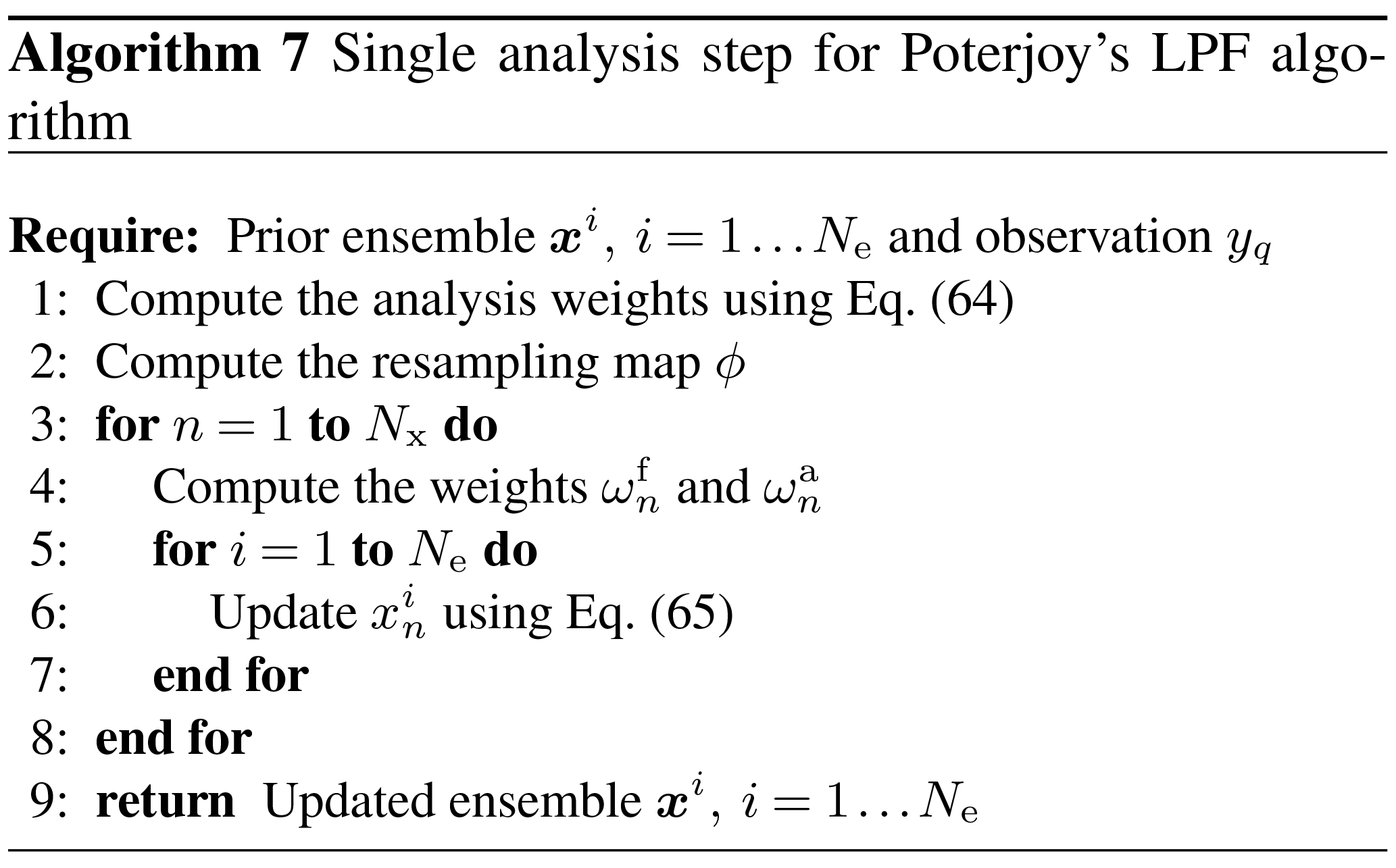
The formulas for the ω∗ weights are summarised in Appendix B. Their detailed derivation can be found in Poterjoy (2016), where ωa and ωf are called r1 and r2. Poterjoy (2016) included a weight inflation parameter in his algorithm that can be ignored to understand how the algorithm works. Moreover, the Ny sequential assimilations are followed by an optional KDDM step. As explained in Sect. 4.4.4, we found the KDDM step to be better suited for the local resampling step of LPFx algorithms. Therefore, we have not included it in our presentation of Poterjoy's LPF.
7.4 A second-order algorithm for the propagation
The second algorithm that we introduce to implement the SO formalism using the “importance, resampling, propagation” scheme is based on the ensemble Kalman particle filter (EnKPF), a Gaussian mixture hybrid ensemble filter designed by Robert and Künsch (2017). In this algorithm, the updated is propagated using second-order moments.
7.4.1 Preliminary: the covariance matrix
Since the update is propagated using second-order moments, one first needs to compute the covariance matrix of the prior ensemble:
In a localisation context, it seems reasonable to use a tapered representation of the covariance. Therefore, we use the covariance matrix Σ defined by
where C is the valid tapering matrix mentioned in Sect. 7.1 (defined using the localisation radius r), and ∘ means the Schur product for matrices.
7.4.2 Step 1: importance and resampling
Using the global unnormalised importance weights Eq. (64), we resample the ensemble in the U region and compute the update . For this resampling step, any resampling algorithm can be used:
-
An adjustment-minimising resampling algorithm can be used to minimise the number of updates that need to be propagated.
-
The resampling algorithms based on OT in ensemble space or in state space, as derived in Sect. 4.4.3 and 4.4.4 can be used. As for the LPFx methods, we expect them to create strong correlations between the prior and the updated ensembles.
7.4.3 Step 2: propagation
For each particle the update on V, , depends on the update on U, , through the linear regression:
where ΣVU and ΣU are submatrices of Σ. The full derivation of Eq. (68) is available in Robert and Künsch (2017). Note that Σ is a Nx×Nx matrix, but only the submatrices ΣVU and ΣU need to be computed.
A single analysis step according to this second-order algorithm is summarised by Algorithm 8 in a generic context, with any resampling algorithm.
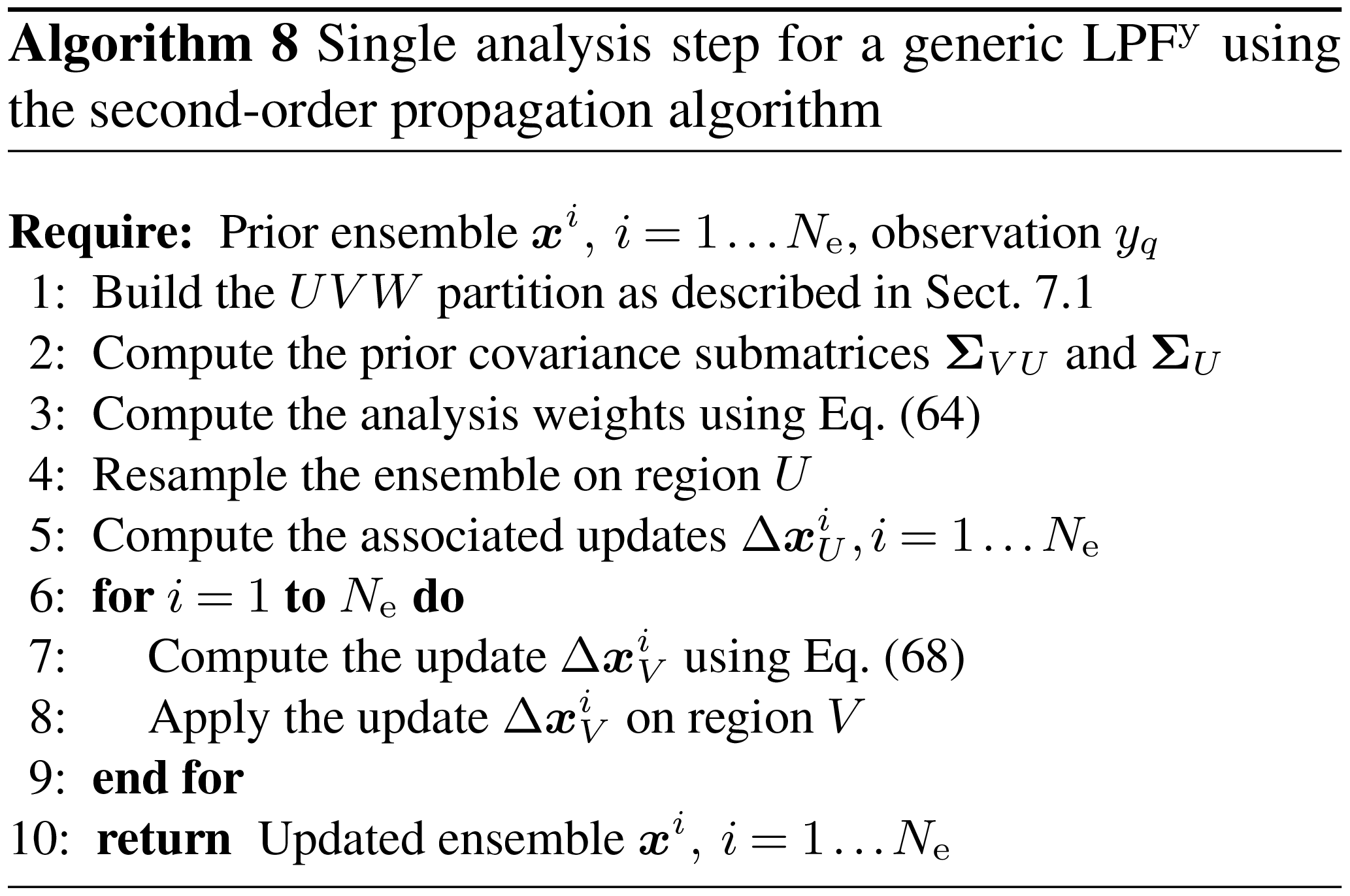
7.5 Summary for the LPFy algorithms
7.5.1 Highlights
In this section, we have introduced a generic SO localisation framework, which we have used to define the LPFys, our second category of LPF methods. We have presented two algorithms, both based on an “importance, resampling, propagation” scheme:
-
The first algorithm is the LPF of Poterjoy (2016). It uses a hybrid scheme between a (global) PF update and the prior ensemble to propagate the update from the observation site to all grid points.
-
The second algorithm was inspired by the EnKPF of Robert and Künsch (2017). It uses tapered second-order moments to propagate the update.
Both algorithms derived in this section include some spatial smoothness in the construction of the updated particles. In Poterjoy's LPF, the smoothness comes from the definition of the ω∗ weights. In the second-order propagation scheme, the smoothness comes from the prior correlations. Therefore, we expect the unphysical discontinuities to be less critical with these algorithms than with the LPFx algorithms, which is why the partition was introduced in the first place.
7.5.2 Numerical complexity
Let NU and NV be the maximum number of grid points in U and V, respectively, and let . The complexity of assimilating one observation using Poterjoy's LPF is
-
𝒪(Ne) to compute the analysis weights Eq. (64) and the resampling map ϕ,
-
𝒪(NeNUV) to compute the ω∗ weights and to propagate the update to the U and V regions.
The complexity of assimilating one observation using the second-order propagation algorithm is the sum of the complexity of computing the update on the U region and on the V region and of applying these updates to the ensemble. The complexity of computing the update on the U region is
-
𝒪(NeNU) when using the adjustment-minimising SU sampling algorithm,
-
when using the optimal ensemble coupling derived in Sect. 4.4.3 with a distance radius rd,
-
𝒪(NUNeNp) when using the anamorphosis derived in Sect. 4.4.4 with a fixed one-dimensional resolution of Np points.
Using Eq. (68), the complexity of computing the update on the V region is
-
to compute ,
-
to apply to all .
Finally, the complexity of applying the update on the U and V regions is 𝒪(NeNUV).
With LPFy algorithms, observations are assimilated sequentially, which means that these algorithms are to be applied Ny times per assimilation cycle. This also means that the LPFy algorithms are, by construction, non-parallel. This issue was discussed by Robert and Künsch (2017): some level of parallelisation could be introduced in the algorithms, but only between observation sites for which the U and V regions are disjoint. That is to say, one can assimilate the observation at several sites in parallel as long as their domains of influence (in which an update is needed) do not overlap. This would require a preliminary geometric step to determine the order in which observation sites are to be assimilated. This step would need to be performed again whenever the localisation radius r is changed. Moreover, when r is large enough, all U and V regions may overlap, and parallelisation is not possible.
7.5.3 Asymptotic limit
By definition of the ω∗ weights, the single analysis step for Poterjoy's LPF is equivalent to the analysis step of the (global) PF for a single observation in the limit r→∞. This is not the case for the algorithm based on the second-order propagation scheme. Indeed, using second-order moments to propagate the update introduces a bias in the analysis. On the other hand, second-order methods are, in general, less sensitive to the curse of dimensionality. Therefore, we expect the algorithm based on the second-order propagation scheme to be able to handle larger values for the localisation radius r than the LPFxs.
7.6 Gathering observation sites into blocks
The LPFys can be extended to the case where observation sites are compounded into small blocks as follows:
-
The unnormalised importance weights Eq. (64) are modified such that they account for all sites inside the block.
-
Any distance that needs to be computed relative to the site of observation yq (for example for the ω∗ weights for Poterjoy's LPF) is now computed relatively to the block centre.
-
In the algorithm based on the second-order propagation scheme, the UVW partition is modified: the U region has to cover all grid points that directly influence every site inside the block.
Gathering observation sites into blocks reduces the number of sequential assimilations from Ny to the number of blocks, hence reducing the computational time per cycle. However, it introduces an additional bias in the analysis. Therefore, we do not use this method in the numerical examples of Sects. 8 and 9.
8.1 Experimental setup
In this section, we illustrate the performance of the LPFy algorithms using twin simulations with the L96 and the BV models. The model specifications for this test series are the same as for the LPFx test series: the L96 model is used in the standard configuration described in Appendix A3, and the BV model is used in the CR configuration described in Appendix A4.1. In a manner consistent with Sects. 5 and 6, the LPFy algorithms are named S(IαPβ)yγ – sampling, importance, resampling, propagation, regularisation, the y exponent meaning that steps in parentheses are performed locally for each observation – with the conventions detailed in Table 3. Table 4 lists all LPFy algorithms tested in this section and reports their characteristics according to the convention of Table 3.
8.1.1 Regularisation jitter
For the same reasons as with LPFxs, jittering the LPFys is necessary to avoid a fast collapse. As we eventually did for the LPFxs, the model is not perturbed (no integration jitter), and regularisation noise is added at the end of each assimilation cycle, either by using the white noise method described by Eq. (45) or by using the coloured noise method described in Sect. 5.8. With the latter method, the local weights required for the computation of the covariance matrix of the regularisation noise are computed with Eq. (29).
Table 3Nomenclature conventions for the S(IαPβ)yγ algorithms. Capital letters refer to the main algorithmic ingredients: “I” for importance, “R” for resampling or regularisation, “T” for transport, and “P” for propagation. Subscripts are used to distinguish the methods in two different ways. Lower-case subscripts refer to explicit concepts used in the method: “s” stands for state space, “c” for colour. Upper-case subscripts refer to the work that inspired the method: “P” stands for Poterjoy (2016) and “RK” for Robert and Künsch (2017). For simplicity, some subscripts are omitted: “amsu” for adjustment-minimising stochastic universal and “w” for white.
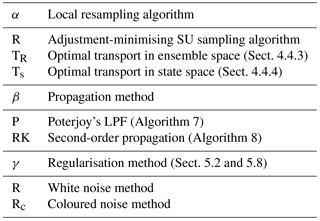
Table 4List of all LPFy algorithms tested in this article. For each algorithm, the main characteristics are reported with appropriate references.
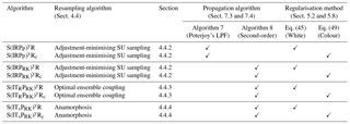
8.1.2 The S(IRPP)yR algorithm and its variant
With the regularisation method described in Sect. 8.1.1, the S(IRPP)yR has three parameters:
-
the ensemble size Ne,
-
the localisation radius r used to compute the ω∗ weights (step 4 of Algorithm 7) as defined by Eqs. (B1) to (B4),
-
the standard deviation s of the regularisation jitter, hereafter simply called “regularisation jitter” to be consistent with the LPFxs.
For each value of the ensemble size Ne, the localisation radius r and the regularisation jitter s are systematically tuned to yield the lowest RMSE score.
As mentioned in Sect. 7.3.2, the original algorithm designed by Poterjoy (2016) included another tuning parameter, the weight inflation, which serves the same purpose as the regularisation jitter. Based on extensive tests in the L96 model with 8 to 128 particles (not shown here), we have found that using weight inflation instead of regularisation jitter always yields higher RMSEs. Therefore, we have not included weight inflation in the S(IRPP)yR algorithm.
In the S(IRPP)yRc algorithm, the regularisation jitter parameter s is replaced by , according to the coloured noise regularisation jitter method. The parameter tuning method is unchanged.
8.1.3 The S(IRPRK)yR algorithm and its variants
With the regularisation method described in Sect. 8.1.1, the S(IRPRK)yR has three parameters:
-
the ensemble size Ne,
-
the localisation radius r used to define the valid tapering matrix C required for the computation of the prior covariance submatrices (step 2 of Algorithm 8) as defined by Eq. (67),
-
the regularisation jitter s.
For each value of the ensemble size Ne, the localisation radius r and the regularisation jitter s are systematically tuned to yield the lowest RMSE score.
When using optimal ensemble coupling for the local resampling (step 4 of Algorithm 8), the local minimisation coefficients are computed using Eq. (35). This gives an additional tuning parameter, the distance radius rd, which is also systematically tuned to yield the lowest RMSE score. When using anamorphosis for the local resampling step, the cumulative density functions of the state variables in the region U are computed in the same way as for LPFx algorithms, with a regularisation bandwidth h=1. Finally, when using the coloured noise regularisation jitter method, the parameter s is replaced by , and the tuning method stays the same.
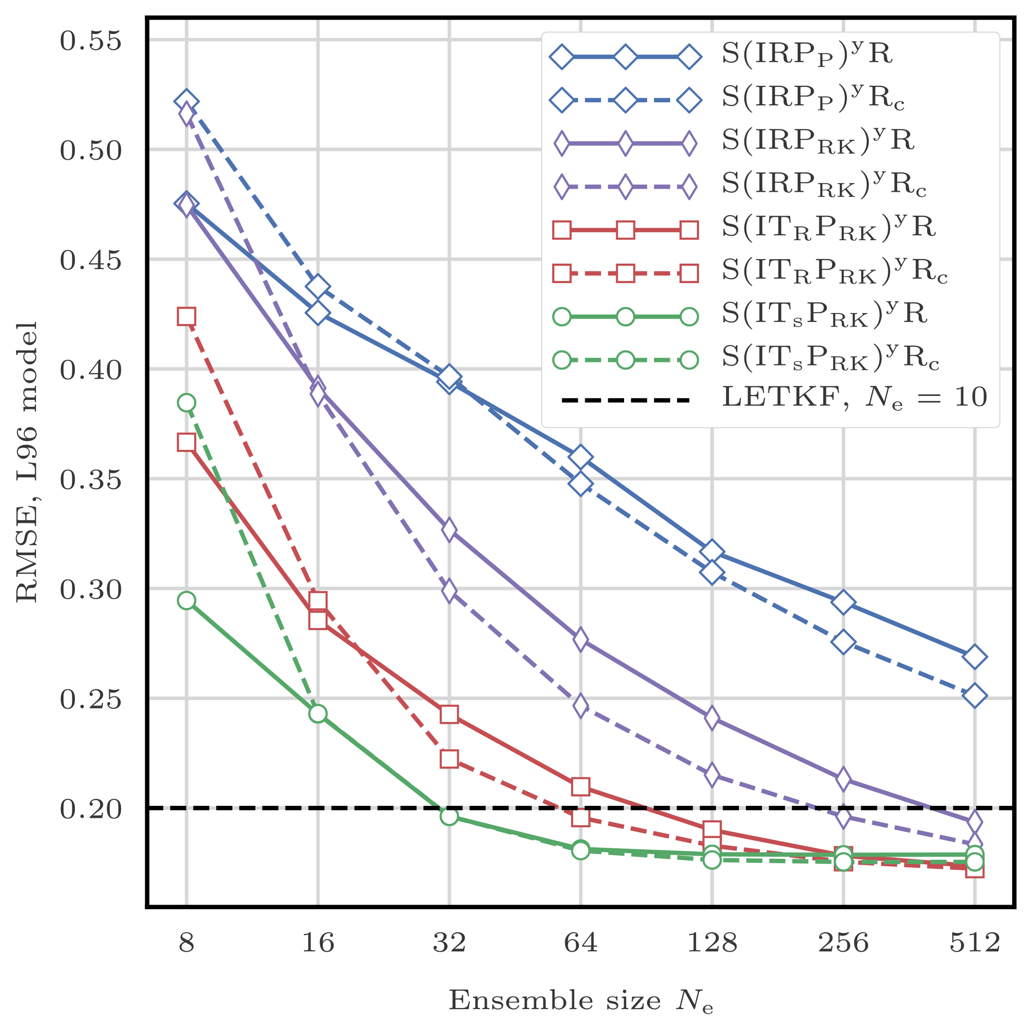
8.2 RMSE scores for the L96 model
The evolution of the RMSE as a function of the ensemble size Ne for the LPFy algorithms with the L96 model is shown in Fig. 20. The RMSEs obtained with the S(IRPP)yR algorithm are comparable to those obtained with the S(IR)xR algorithm. When using the second-order propagation method, the RMSEs are, as expected, significantly lower. The algorithm is less sensitive to the curse of dimensionality than the LPFx algorithms: optimal values of the localisation radius r are significantly larger and less regularisation jitter s is required. Similarly to the LPFxs, combining the second-order propagation method with OT-based resampling algorithms (optimal ensemble coupling or anamorphosis) yields important gains in RMSE scores as a consequence of the minimisation of the update in the region U that needs to be propagated to the region V. With a reasonable number of particles (e.g. 64 for the S(ITsPRK)yR algorithm), the scores are significantly lower than those obtained with the reference EnKF implementation (the ETKF). Finally, we observe that using the coloured noise regularisation jitter method improves the RMSEs for large ensembles when the local resampling step is performed with the SU sampling algorithm, in a similar way as for the LPFxs. However when the local resampling step is performed with optimal ensemble coupling or with anamorphosis, the coloured noise regularisation jitter method barely improves the RMSEs.
8.3 RMSE scores for the BV model
The evolution of the RMSE as a function of the ensemble size Ne for the LPFy algorithms with the BV model is shown in Fig. 21. Most of the conclusions drawn with the L96 model remain true with the BV model. However, in this case, as the ensemble size Ne grows, the RMSE decreases significantly more slowly for the S(IRPP)yR and the S(IRPP)yRc algorithms than for the other algorithms. Finally, with an ensemble size Ne≥64 particles, the S(ITsPRK)yR and the S(ITsPRK)yRc algorithms yield RMSEs almost equivalent to those of the reference LETKF implementation.
9.1 Experimental setup
In this section, we illustrate the performance of a selection of LPFxs and LPFys using twin simulations of the BV model in the high-resolution (HR) configuration described in Appendix A4.2. Using this configuration yields a higher dimensional DA problem (Nx=65 536 and Ny=4096) for which the analysis step is too costly to perform exhaustive tests. Therefore, in this section, we take Ne=32 ensemble members and we monitor the time evolution of the analysis RMSE during 501 assimilation steps.
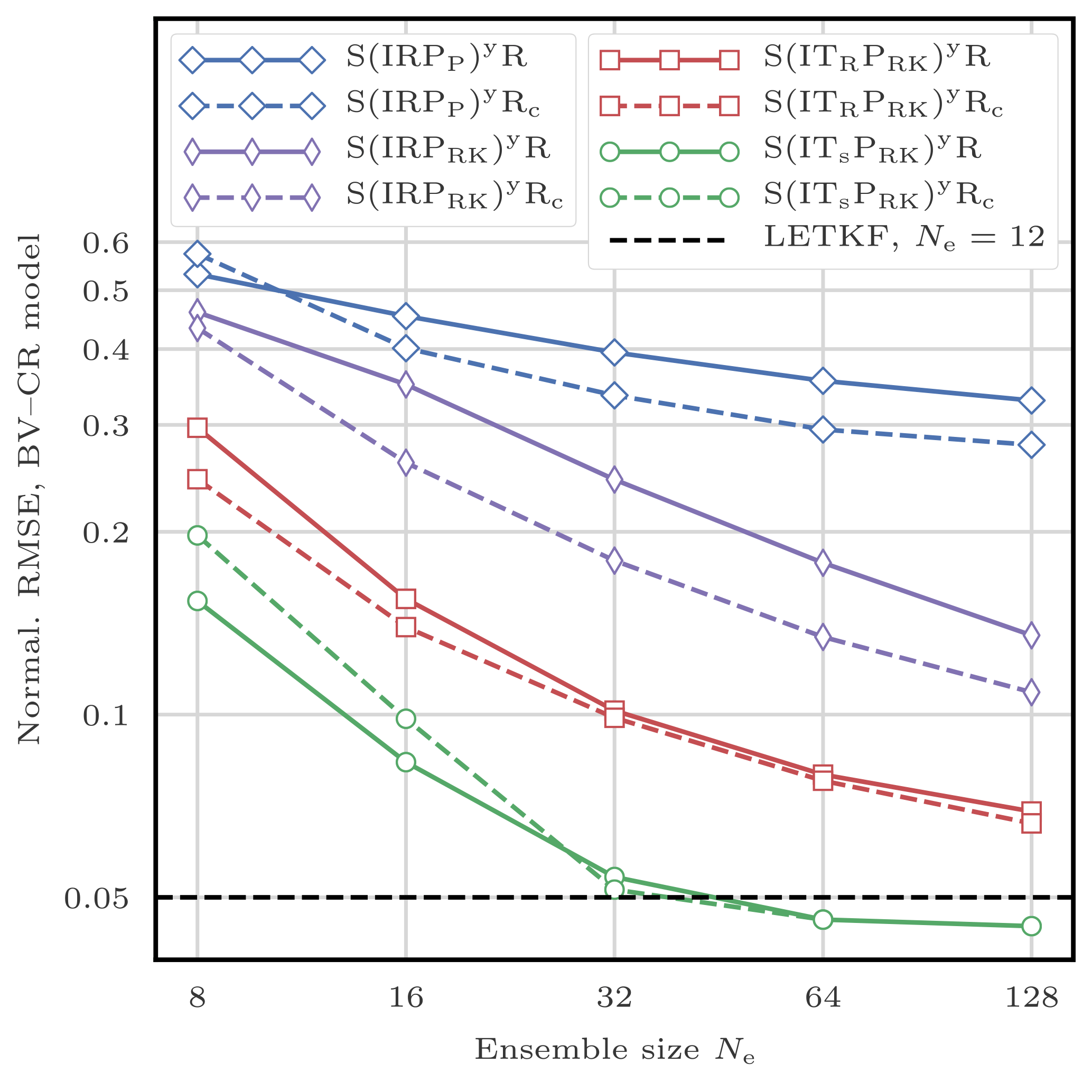
Figure 21RMSE as a function of the ensemble size Ne for the LPFys. The scores are displayed in units of the observation standard deviation σ.
Table 5Characteristics of the algorithms tested with the BV model in the HR configuration (Fig. 22). The LPFxs use zero integration jitter (q=0) and Nb=Nx blocks of size 1 grid point. The LPFys also use zero integration jitter (q=0). For the LETKF, the optimal multiplicative inflation is reported in the regularisation jitter column. For the S(IR)xSPMRc algorithm, the optimal regularisation jitter bandwidth is reported in the regularisation jitter column as well. The average RMSE is computed over the final 300 assimilation steps and is given in units of the observation standard deviation σ. The wall-clock computational time is the average time spent per analysis step. The simulations are performed on a single core of a double Intel Xeon E5-2680 platform (for a total of 24 cores). For comparison, the average time spent per forecast (Δt=0.5) for the 32-member ensemble is 0.94 s. The bold font indicates that the local analyses can be carried out in parallel, allowing a theoretical gain in computational time of up to a factor of 65 536. For these algorithms, the average time spent per analysis step for the parallelised runs on this 24-core platform, as well as the acceleration factor, are reported in the last column.
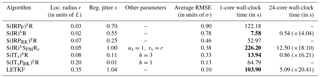
As with the CR configuration, all geometrical considerations (blocks and domains, UVW partition, etc.) use the Euclidean distance of the underlying physical space.
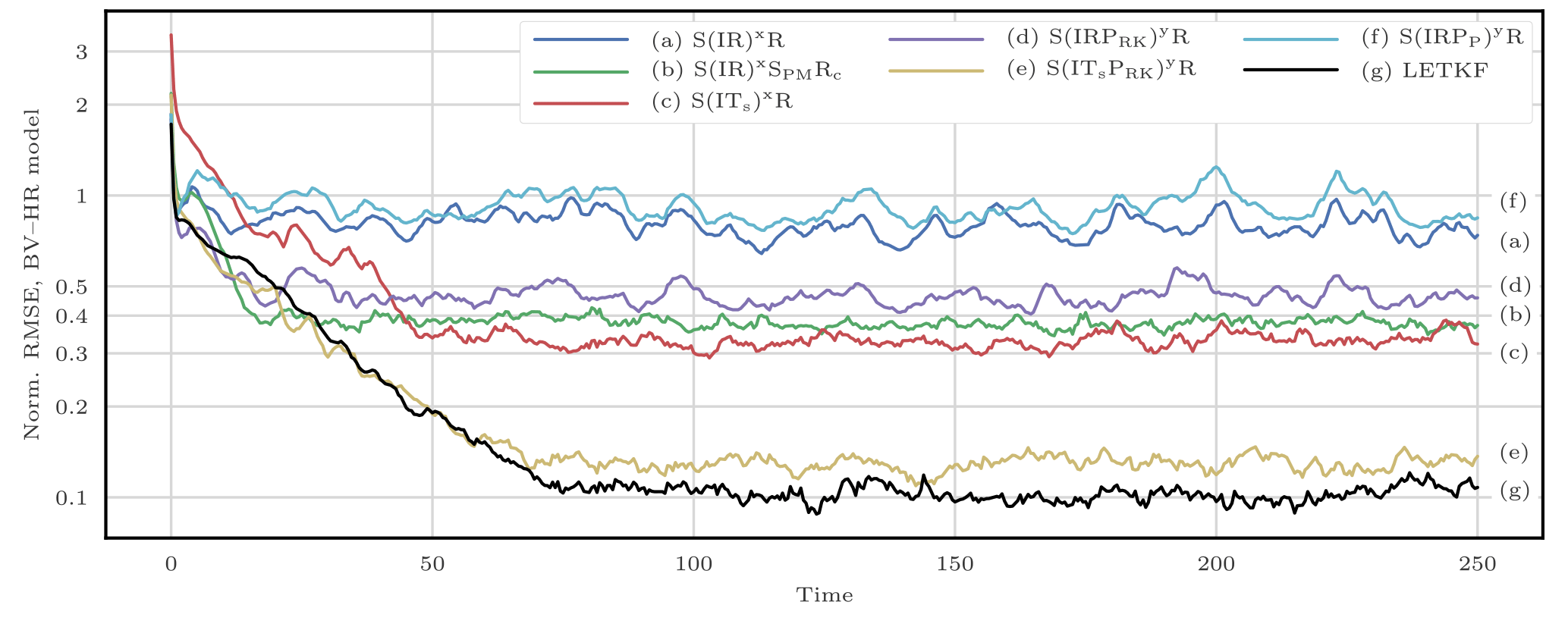
9.2 Algorithm specifications
For this test series, the selection of algorithms is listed in Table 5. Each algorithm uses the same initial ensemble obtained as follows:
where u and the ui are random vectors whose coefficients are distributed according to a normal law. Such an ensemble is not very close to the truth (in terms of RMSE), and its spread is large enough to reflect the lack of initial information. The LPFs use zero integration jitter and Nb=Nx blocks of size 1 grid point. Approximate optimal values for the localisation radius r and the regularisation jitter (s or depending on the potential colourisation of the noise) are found using several twin experiments with a few hundred assimilation cycles (not shown here). The localisation radius r and the multiplicative inflation for the LETKF are found in a similar manner. When using OT in state space, we only test a few values for the regularisation bandwidth h. When using the smoothing-by-weights method, we take the smoothing strength αs=1 and the smoothing radius rs is set to be equal to the localisation radius r.
9.3 RMSE time series
Figure 22 shows the evolution of the instantaneous analysis RMSE for the selected algorithms. Approximate optimal values for the tuning parameters, alongside the average analysis RMSE, computed over the final 300 assimilation steps and wall-clock computational times, are reported in Table 5. In terms of RMSE scores, the ranking of the methods is unchanged, and most of the conclusions for this test series are the same as with the CR configuration.
Thanks to the uniformly distributed observation network, the posterior probability density functions are close to Gaussian. Therefore the LETKF algorithm can efficiently reconstruct a good approximation of the true state. As expected with this high-dimensional DA problem, the algorithms using a second-order truncation (the LETKF and the S(I∗PRK)yR algorithms) are more robust. Optimal values of the localisation radius are qualitatively large, which allows for a better reconstruction of the system dynamics.
For the S(IR)xR and the S(IRPP)xR algorithms, the optimal localisation radius r needs to be very small to counteract the curse of dimensionality. With such small values for r, the local domain of each grid point contains only 4 to 13 observation sites. This is empirically barely enough to reconstruct the true state with an RMSE score lower than the observation standard deviation σ. As in the previous test series, using OT-based local resampling methods or the smoothing-by-weights step yields significantly lower RMSEs. The RMSEs of the S(ITs)xR and the S(IR)xSPMRc algorithms, though not as good as that of the LETKF algorithm, show that the true state is reconstructed with an acceptable accuracy. The RMSEs of the S(ITsPRK)yR and the LETKF algorithms are almost comparable. Depending on the algorithm, the conditioning to the initial ensemble more or less quickly vanishes.
Without parallelisation, we observe that the Nx local analyses of the LPFxs are almost always faster than both the Nx local analyses of the LETKF and the Ny sequential assimilations of the LPFys. The second-order propagation algorithm is slower because of the linear algebra involved in the method. Poterjoy's propagation algorithm is slower because computing the ω∗ weights is numerically expensive. The LETKF is slower because of the matrices inversion in ensemble space. Finally, the S(IR)xSPMRc algorithm is even slower because, in this two-dimensional model, the smoothing-by-weights step is numerically very expensive.
The difference between the LPFxs and the LPFys is even more visible on our 24-core platform. The LPFys are not parallel, that is why they are more than 70 times slower than the fastest LPFxs.
The curse of dimensionality is a rather well-understood phenomenon in the statistical literature, and it is the reason why PF methods fail when applied to high-dimensional DA problems. We have recalled the main results related to weight degeneracy of PFs, and why the use of localisation can be used as a solution. Yet implementing localisation in PF analysis raises two major issues: the gluing of locally updated particles and potential physical imbalance in the updated particles. Adequate solutions to these issues are not obvious, witness the few but dissimilar LPF algorithms developed in the geophysical literature. In this article we have proposed a theoretical classification of LPF algorithms into two categories. For each category, we have presented the challenges of local particle filtering and have reviewed the ideas that lead to practical implementation of LPFs. Some of them, already in the literature, have been detailed and sometimes generalised, while others are new in this field and yield improvements in the design of LPF methods.
With the LPFx methods, the analysis is localised by allowing the analysis weights to vary over the grid points. We have shown that this yields an analysis pdf from which only the marginals are known. The local resampling step is mandatory for reconstructing global particles that are obtained by assembling the locally updated particles. The quality of the updated ensemble directly depends on the regularity of the local resampling. This is related to unphysical discontinuities in the assembled particles. Therefore we have presented practical methods to improve the local resampling step by reducing the unphysical discontinuities.
In the LPFy methods, localisation is introduced more generally in the conditional density for one observation by the means of a state partition. The goal of the partition is to build a framework for local particle filtering without the discontinuity issue inherent to LPFxs. However, this framework is irreconcilable with algorithms based on pure “importance, resampling” methods. We have shown how two hybrid methods could yet be used as an implementation of this framework. Besides, we have emphasised the fact that with these methods, observations are, by construction, assimilated sequentially, which is a great disadvantage when the number of observations in the DA problem is high.
With localisation, a bias is introduced in the LPF analyses. We have shown that, depending on the localisation parameterisation, some methods can yield an analysis step equivalent to that of global PF methods, which are known to be asymptotically Bayesian.
We have implemented and systematically tested the LPF algorithms with twin simulations of the L96 model and the BV model. A few observations could be made from these experiments. With these models, implementing localisation is simple and works as expected: the LPFs yield acceptable RMSE scores, even with small ensembles, in regimes where global PF algorithms are degenerate. In terms of RMSEs, there is no clear advantage of using Poterjoy's propagation method (designed to avoid unphysical discontinuities) over the (simpler) LPFx algorithms, which have a lower computational cost. As expected, algorithms based on the second-order propagation method are less sensitive to the curse of dimensionality and yield the lowest RMSE scores. We have shown that using OT-based local resampling methods always yields important gains in RMSE scores. For the LPFxs, it is a consequence of mitigating the unphysical discontinuities introduced in the local resampling step. For the LPFys, it is a consequence of the minimisation of the update at the observation site that needs to be propagated to nearby grid points.
The successful application of the LPFs to DA problems with a perfect model is largely due to the use of regularisation jitter. Using regularisation jitter introduces an additional bias in the analysis alongside an extra tuning parameter. For our numerical experiments, we have introduced two jittering method: either using regularisation noise with fixed statistical properties (white noise) or by scaling the noise with the ensemble anomalies (coloured noise). We have discussed the relative performance of each method and concluded that there is room for improvement in the design of regularisation jitter methods for PFs.
In conclusion, introducing localisation in the particle filter is a relatively young topic that can benefit from more theoretical and practical developments.
First, the resampling step is the main ingredient in the success, or failure, of an LPF algorithm. The approaches based on optimal transport offer an elegant and quite efficient framework to deal with the discontinuity issue inherent to local resampling. However, the algorithms derived in this article could be improved. For example, it would be desirable to avoid the systematic reduction to one-dimensional problems when using optimal transport in state space. Besides this, other frameworks for local resampling based on other theories could be conceived.
Second, the design of the regularisation jitter methods can be largely improved. Regularisation jitter is mandatory when the model is perfect. Even with stochastic models, it can be beneficial, for example, when the magnitude of the model noise is too small for the LPFs to perform well. Ideally, the regularisation jitter methods should be adaptive and built concurrently with the localisation method.
Third, with the localisation framework presented in this article, one cannot directly assimilate non-local observations. The ability to assimilate non-local observations becomes increasingly important with the prominence of satellite observations.
Finally, our numerical illustration with the BV model in the HR configuration is successful and shows that the LPF algorithms have the potential to work with high-dimensional systems. Nevertheless further research is needed to see if the LPFs can be used with realistic models. Such an application would require an adequate definition of the model noise and the observation error covariance matrix. Even if the local resampling methods have been designed to minimise the unphysical discontinuities, this will have to be carefully checked, because this is a critical point in the success of the LPF. Last, the regularisation jitter method has to be chosen and tuned in adequation with the model noise. In particular, the magnitude of the jitter will almost certainly depend on the state variable.
No data sets were used in this article.
A1 The Gaussian linear model
The Gaussian linear model is the simplest model with size Nx whose prior distribution is
whose transition distribution is
and whose observation distribution is
A2 Generic model with Gaussian additive noise
The Gaussian linear model can be generalised to include nonlinearity in the model ℳ and in the observation operator ℋ. In this case, the transition distribution is
and the observation distribution is
where Q and R are the covariance matrices of the additive model and observation errors.
A3 The Lorenz 1996 model
The Lorenz 1996 model (Lorenz and Emanuel, 1998) is a low-order one-dimensional discrete chaotic model whose evolution is given by the following set of ODEs:
where the indices are to be understood with periodic boundary conditions: , , and , and where the system size Nx can take arbitrary values. These ODEs are integrated using a fourth-order Runge–Kutta method with a time step of a 0.05 time unit.
In the standard configuration, Nx=40 and F=8, which yields a chaotic dynamics with a doubling time around a 0.42 time unit. The observations are given by
and the time interval between consecutive observations is a Δt=0.05 time unit, which represents 6 h of real time and corresponds to a model autocorrelation around 0.967.
A4 The barotropic vorticity model
The barotropic vorticity model describes the evolution of the vorticity field of a two-dimensional incompressible homogeneous fluid in the x1−x2 plane. The time evolution of the unknown vorticity field ζ is governed by the scalar equation
and ζ is related to the stream function ψ through
In these equations, J(ψ, ζ) is the advection of the vorticity by the stream, defined as
where is the friction coefficient, is the diffusion coefficient, and F is the forcing term, which may depend on x1, x2, and t. The system is characterised by homogeneous two-dimensional turbulence. The friction extracts energy at large scales, the diffusion dissipates vorticity at small scales and the forcing injects energy in the system. The number of degrees of freedom in this model can be roughly considered to be proportional to the number of vortices (Chris Snyder, personal communication, 2012).
The equations are solved with P2 grid points regularly distributed over the simulation domain [0, L]2 with doubly periodic boundary conditions. Our time integration method is based on a semi-Lagrangian solver with a constant time step δt as follows:
-
At time t, solve Eq. (A9) for ψ.
-
At time t, compute the advection velocity with second-order centred finite differences of the field ψ.
-
The advection of ζ during t and t+δt is computed by applying a semi-Lagrangian method to the left-hand side of Eq. (A8). The solver cannot be more precise than first-order in time, since the value of ψ is not updated during this step. Therefore, our semi-Lagrangian solver uses the first-order forward Euler time integration method. The interpolation method used is the cubic convolution interpolation algorithm, which yields a third-order precision with respect to the spatial discretisation. In this step, the right-hand side of Eq. (A8) is ignored.
-
Integrate ζ from t to t+δt by solving Eq. (A8) with an implicit first-order time integration scheme in which the advection term is the one computed in the previous step.
For the numerical experiments of this article, the spatial discretisation is fine enough that the spatial interpolation error in the semi-Lagrangian step is negligible when compared to the time integration error. As a consequence, the overall integration method is first-order in time. For the DA experiments with this model, we define and use two configurations.
A4.1 Coarse-resolution configuration
The coarse-resolution configuration is based on the following set of physical parameters:
The deterministic forcing is given by
and the space–time discretisation is
which yields . The spatial discretisation is enough to allow a reasonable description of a few (typically five to ten) vortices inside the domain. The temporal discretisation is empirically enough to ensure the stability of the integration method and allows a fast computation of the trajectory. The physical parameters are chosen to yield a proper time evolution of the vorticity ζ.
The initial true vorticity field for the DA twin experiments is the vorticity obtained after a run of 100 time units starting from a random, spatially correlated field. The system is partially observed on a regular square mesh with one observation site for every 2 grid points in each direction, i.e. Ny=256 observation sites for Nx=1024 grid points. At every cycle k, the observation at site is given by
with σ=0.3, about one tenth of the typical vorticity variability. The time interval between consecutive observations is a Δt=0.5 time unit, which was chosen to match approximately the model autocorrelation of 0.967 of the L96 model in the standard configuration.
We have checked that the vorticity flow remains stationary over the total simulation time of our DA twin experiments chosen to be 104Δt. Due to the forcing F, the flow remains uniformly and stationarily turbulent during the whole simulation. Compared to other experiments with the barotropic vorticity model (e.g. van Leeuwen and Ades, 2013; Ades and van Leeuwen, 2015; Browne, 2016), Δt is smaller and σ is larger, but the number of vortices is approximately the same, with much fewer details.
A4.2 High-resolution configuration
For the high-resolution configuration, the physical parameters are
The deterministic forcing is given by
and the space–time discretisation is
which yields . Compared to the coarse-resolution configuration, this set of parameters yields a vorticity field with more vortices (typically several dozens). The associated DA problem therefore has many more apparent or effective degrees of freedom. The initial true vorticity field for the DA twin experiments is the vorticity obtained after a run of 100 time units starting from a random, spatially correlated field. The system is partially observed on a regular square mesh with one observation site for every 4 grid points in each direction, i.e. Ny=4096 observation sites for Nx=65 536 grid points. At every cycle k, the observation at site is given by
and we keep the values Δt=0.5 time units and σ=0.3 from the coarse-resolution configuration. We have checked that the vorticity flow remains stationary over the total simulation time of our DA twin experiments chosen to be 500Δt. Due to the forcing F, the flow remains uniformly and stationarily turbulent during the whole simulation.
Following Poterjoy (2016), we derived the following formulas for the ω∗ weights required in the propagation step of Poterjoy's LPF described in Sect. 7.3.2:
where W and cn are ancillary variables, α is the constant used for the computation of the local weights (see Eq. 28), G is the tapering function, dq, n is the distance between the qth observation site and the nth grid point, r is the localisation radius, is the mean, and σn the standard deviation of the weighted ensemble . The particles are then updated using Eq. (65).
In Poterjoy (2016), the probability density functions are implicitly normalised, such that the constant α is 1. Therefore, our update Eqs. (B1) to (B4) are equivalent to the update Eqs. (A10), (A11), (A5), and (A3) derived by Poterjoy (2016). Note that there is a typing mistake which renders one update equation in Algorithm 1 of Poterjoy (2016) incorrect (last equation on p. 66).
As a complement to the mildly nonlinear test series of Sects. 5, 6, 8, and 9, we provide here a strongly nonlinear test series. We consider the L96 model in the standard configuration described in Appendix A3, with the only difference being that the Ny=Nx observations at each assimilation cycle are now given by
This strongly nonlinear configuration has been used, e.g. by Poterjoy (2016).
Similarly to the mildly nonlinear test series, the distance between the truth and the analysis is measured with the average analysis RMSE. The runs are 9×10³Δt long, with an additional 103Δt spin-up period. Optimal values for the tuning parameters of each algorithms are found using the same method as for the mildly nonlinear test series. Figure C1 shows the evolution of the RMSE as a function of the ensemble size Ne for the LETKF and for the main LPFx and LPFy algorithms.
As expected in this strongly nonlinear test series, the EnKF fails at accurately reconstructing the true state. By contrast, all LPFs yield, at some point, an RMSE under σ=1 (the observation standard deviation). Regarding the ranking of the methods, most conclusions from the mildly nonlinear case remain true. The best RMSE scores are obtained with algorithms using OT-based resampling methods. Combining the smoothing-by-weights method with the coloured noise regularisation jitter method yields almost equally good scores as the LPFx algorithms using OT. Finally, using the second-order propagation method yields the lowest RMSEs, despite the non-Gaussian error distributions that result from nonlinearities.
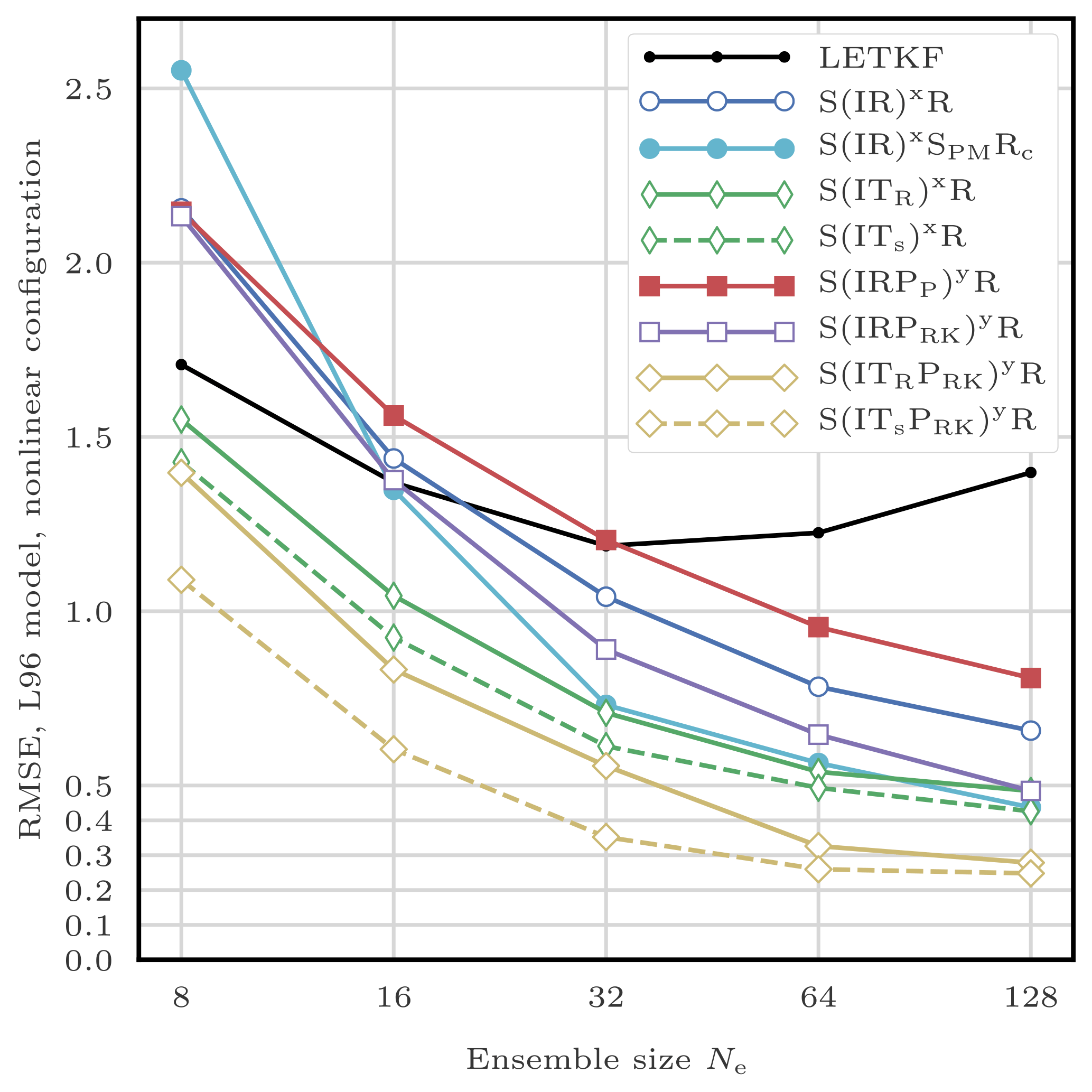
Figure C1RMSE as a function of the ensemble size Ne for the LETKF and the main LPFs, with the L96 model in the strongly nonlinear configuration. Note that the ultimate increase of the RMSE of the LETKF with the ensemble size could have been avoided by using random rotations in ensemble space.
As a complement to the RMSE test series, we compute rank histograms of the ensembles (Anderson, 1996; Hamill, 2001). For this experiment, the DA problem is the same as the one in Sects. 5 and 8: the L96 model is used in its standard configuration.
Table D1Rank histograms computed with the L96 model in the standard configuration (see Appendix D). All LPFs use zero integration jitter (q=0). The localisation radii are given in number of grid points. For the ETKF, the optimal multiplicative inflation is reported in the regularisation jitter column. The bold font in the RMSE column indicates that the algorithm parameters have been tuned to yield the lowest RMSE score. The first column indicates the corresponding panel in Fig. D1.
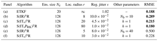

Figure D1Rank histograms for the selection of algorithms detailed in Table D1. The frequency is normalised by Ne+1 (the number of bins).
Several algorithms are selected with characteristics detailed in Table D1. The histograms are obtained separately for each state variable by computing the rank of the truth in the unperturbed analysis ensemble (i.e. the analysis ensemble before the regularisation step for the LPFs). To ensure the convergence of the statistical indicators, the runs are 105Δt long with a 103Δt spin-up period. The mean histograms (averaged over the state variables) are reported in Fig. D1.
The histogram of the EnKF is quite flat in the middle, and its edges reflect a small overdispersion. The histogram of the tuned S(IR)xR algorithm is characterised by a large hump, showing that the ensemble is overdispersive. At the same time, the high frequencies at the edges show that the algorithm yields a poor representation of the distribution tails (as most PF methods). The overdispersion of the ensemble is a consequence of the fact that the parameters have been tuned to yield the best RMSE score, regardless of the flatness of the rank histogram. With a different set of parameter, the untuned S(IR)xR algorithm yields a rank histogram much flatter. In this case, the regularisation jitter is lower (which explains the fact that the ensemble is less overdispersive) and the localisation radius smaller (to avoid the filter divergence). Of course, the RMSE score for the untuned S(IR)xR algorithm is higher than for its tuned version. Similar conclusions can be found with the histograms of the tuned and untuned S(ITs)xR algorithm. Note that in this case the histograms are significantly flatter than with the S(IR)xR algorithm. Finally, the histogram of the (tuned) S(ITsPRK)yR is remarkably flat.
In summary, the rank histograms of the LPFs are in general rather flat. The ensemble are more or less overdispersive; this is a consequence of the use of regularisation jitter, necessary for avoiding the filter divergence. As most PF methods, the LPFs yield a poor representation of the distribution tails.
We describe here the multinomial and the SU sampling algorithms, which are the most common resampling algorithms. In this algorithms, highly probable particles are selected and duplicated, while particles with low probability are discarded. Algorithms 9 and 10 describe how to construct the resampling map ϕ according to the multinomial resampling and the SU sampling algorithms, respectively. The resampling map ϕ is the map such that ϕ(i) is the index of the ith particle selected for resampling.
Both algorithms only require the cumulative weights ci that can easily be obtained from the importance weights wi using
and both algorithms use random number(s) generated from 𝒰(0, 1), the uniform distribution over the interval [0, 1]. Because of these random numbers, both algorithms introduce sampling noise. Moreover, it can be shown that the SU sampling algorithm has the lowest sampling noise (see, e.g. van Leeuwen, 2009).
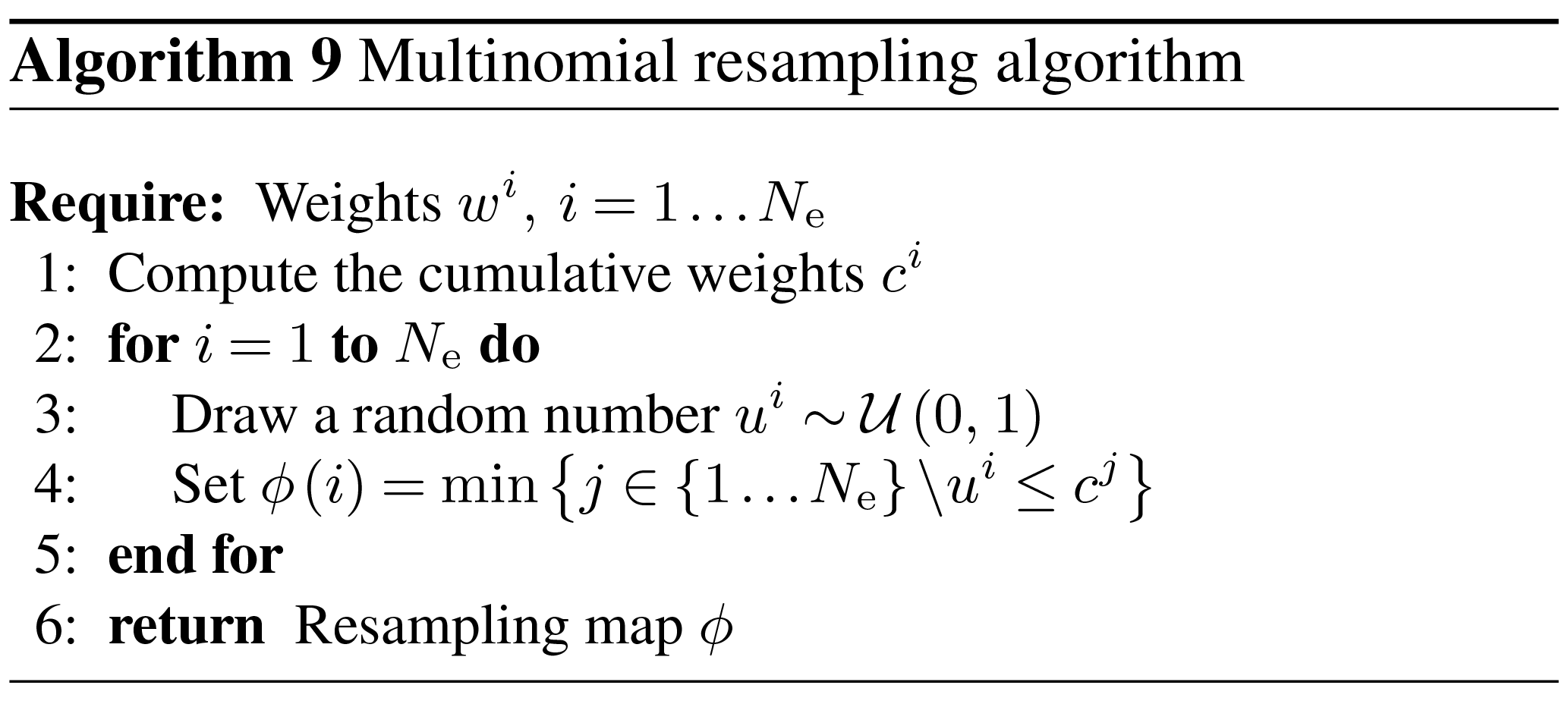
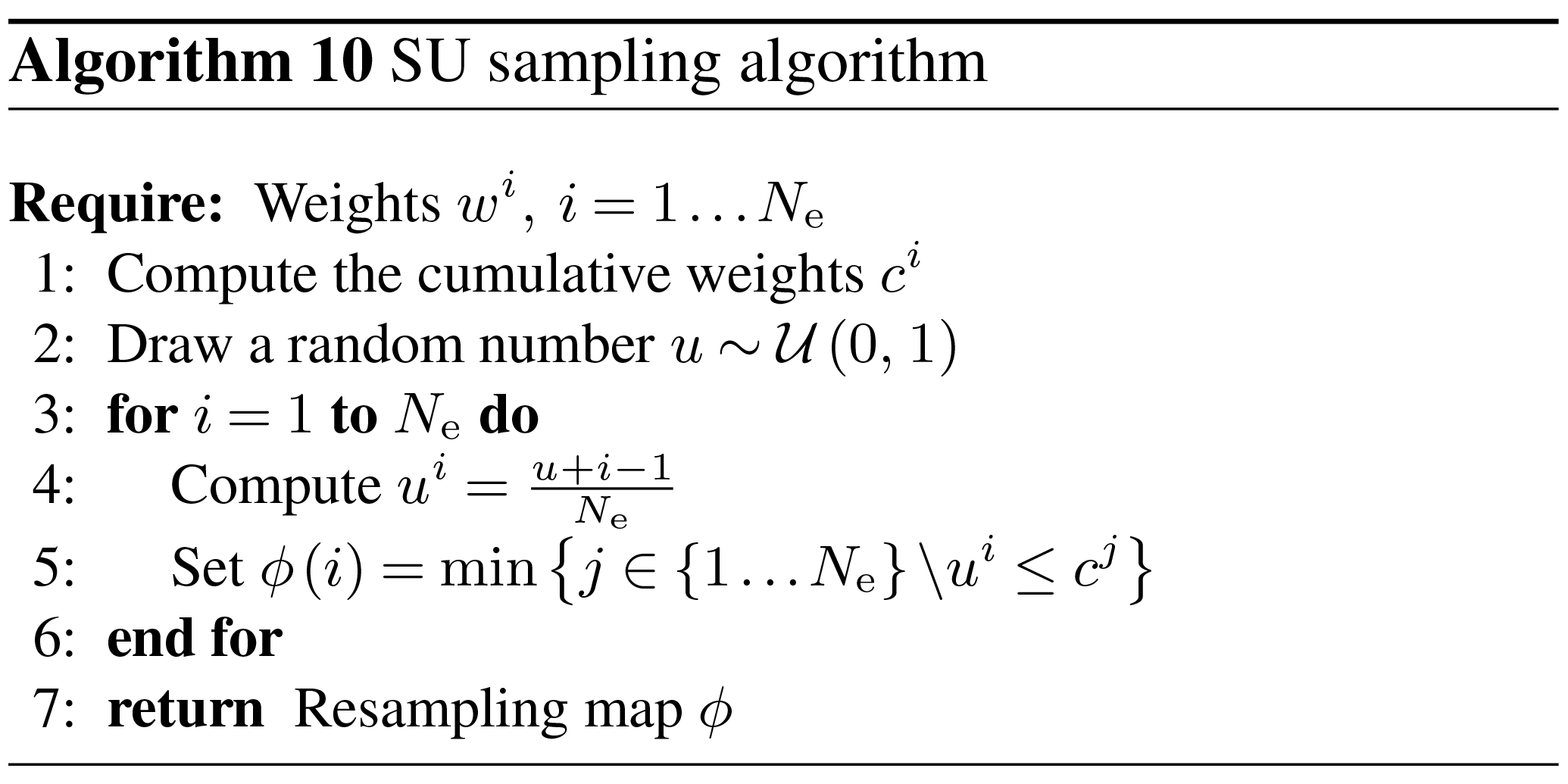
AF and MB have made an equally substantial, direct, and intellectual contribution to all three parts of the work: overview of the literature, algorithm development, and numerical experiments. Both authors have prepared the manuscript and approved it for publication.
The authors declare that they have no conflict of interest.
This article is part of the special issue “Numerical modeling, predictability and data assimilation in weather, ocean and climate: A special issue honoring the legacy of Anna Trevisan (1946–2016)”. It is not associated with a conference.
The authors thank the editor, Olivier Talagrand, and three reviewers, Stephen G. Penny and two anonymous
reviewers, for their useful comments, suggestions and
thorough reading of the manuscript.
The authors are grateful to Patrick Raanes for enlightening debates and to Sebastian Reich for suggestions.
CEREA is a member of Institut Pierre–Simon Laplace (IPSL).
Edited by: Olivier Talagrand
Reviewed by: Stephen G. Penny and two anonymous referees
Acevedo, W., de Wiljes, J., and Reich, S.: Second-order accurate ensemble transform particle filters, SIAM J. Sci. Comput., 39, A1834–A1850, https://doi.org/10.1137/16M1095184, 2017. a
Ades, M. and van Leeuwen, P. J.: The equivalent-weights particle filter in a high-dimensional system, Q. J. Roy. Meteor. Soc., 141, 484–503, https://doi.org/10.1002/qj.2370, 2015. a, b, c
Anderson, J. L.: A Method for Producing and Evaluating Probabilistic Forecasts from Ensemble Model Integrations, J. Climate, 9, 1518–1530, https://doi.org/10.1175/1520-0442(1996)009<1518:AMFPAE>2.0.CO;2, 1996. a
Apte, A. and Jones, C. K. R. T.: The impact of nonlinearity in Lagrangian data assimilation, Nonlin. Processes Geophys., 20, 329–341, https://doi.org/10.5194/npg-20-329-2013, 2013. a
Arulampalam, M. S., Maskell, S., Gordon, N., and Clapp, T.: A tutorial on particle filters for online nonlinear non-Gaussian Bayesian Tracking, IEEE T. Signal Proces., 50, 174–188, https://doi.org/10.1109/78.978374, 2002. a
Bengtsson, T., Snyder, C., and Nychka, D.: Toward a nonlinear ensemble filter for high-dimensional systems, J. Geophys. Res., 108, 8775, https://doi.org/10.1029/2002JD002900, 2003. a
Bishop, C. H., Etherton, B. J., and Majumdar, S. J.: Adaptive Sampling with the Ensemble Transform Kalman Filter. Part I: Theoretical Aspects, Mon. Weather Rev., 129, 420–436, https://doi.org/10.1175/1520-0493(2001)129<0420:ASWTET>2.0.CO;2, 2001. a
Bocquet, M. and Sakov, P.: An iterative ensemble Kalman smoother, Q. J. Roy. Meteor. Soc., 140, 1521–1535, https://doi.org/10.1002/qj.2236, 2014. a
Bocquet, M., Pires, C. A., and Wu, L.: Beyond Gaussian statistical modeling in geophysical data assimilation, Mon. Weather Rev., 138, 2997–3023, https://doi.org/10.1175/2010MWR3164.1, 2010. a, b, c, d, e, f
Bocquet, M., Raanes, P. N., and Hannart, A.: Expanding the validity of the ensemble Kalman filter without the intrinsic need for inflation, Nonlin. Processes Geophys., 22, 645–662, https://doi.org/10.5194/npg-22-645-2015, 2015. a
Browne, P. A.: A comparison of the equivalent weights particle filter and the local ensemble transform Kalman filter in application to the barotropic vorticity equation, Tellus A, 68, 30466, https://doi.org/10.3402/tellusa.v68.30466, 2016. a, b
Chen, Z.: Bayesian filtering: From Kalman filters to particle filters, and beyond, Statistics, 182, 1–69, https://doi.org/10.1080/02331880309257, 2003. a
Cheng, Y. and Reich, S.: Assimilating data into scientific models: An optimal coupling perspective, in: Nonlinear Data Assimilation, vol. 2 of Frontiers in Applied Dynamical Systems: Reviews and Tutorials, 75–118, Springer International Publishing, https://doi.org/10.1007/978-3-319-18347-3, 2015. a, b
Chorin, A. J. and Tu, X.: Implicit sampling for particle filters, P. Natl. Acad. Sci. USA, 106, 17249–17254, https://doi.org/10.1073/pnas.0909196106, 2009. a, b
Chorin, A. J., Morzfeld, M., and Tu, X.: Implicit particle filters for data assimilation, Comm. App. Math. Com. Sc., 5, 221–240, https://doi.org/10.2140/camcos.2010.5.221, 2010. a, b
Chustagulprom, N., Reich, S., and Reinhardt, M.: A Hybrid Ensemble Transform Particle Filter for Nonlinear and Spatially Extended Dynamical Systems, SIAM/ASA Journal on Uncertainty Quantification, 4, 592–608, https://doi.org/10.1137/15M1040967, 2016. a, b, c, d
Crisan, D. and Doucet, A.: A survey of convergence results on particle filtering methods for practitioners, IEEE T. Signal Proces., 50, 736–746, https://doi.org/10.1109/78.984773, 2002. a, b
Dezső, B., Jüttner, A., and Kovács, P.: LEMON – an Open Source C++ Graph Template Library, Electronic Notes in Theoretical Computer Science, 264, 23–45, https://doi.org/10.1016/j.entcs.2011.06.003, 2011. a
Doucet, A., Godsill, S., and Andrieu, C.: On sequential Monte Carlo sampling methods for Bayesian filtering, Stat. Comput., 10, 197–208, https://doi.org/10.1023/A:1008935410038, 2000. a, b, c, d, e
Doucet, A., de Freitas, N., and Gordon, N. (Eds.): Sequential Monte Carlo Methods in Practice, Springer-Verlag New York Inc., https://doi.org/10.1007/978-1-4757-3437-9, 2001. a
Evensen, G.: Sequential data assimilation with a nonlinear quasi-geostrophic model using Monte Carlo methods to forecast error statistics, J. Geophys. Res., 99, 10143–10162, https://doi.org/10.1029/94JC00572, 1994. a
Evensen, G.: The Ensemble Kalman Filter: theoretical formulation and practical implementation, Ocean Dynam., 53, 343–367, https://doi.org/10.1007/s10236-003-0036-9, 2003. a, b
Gaspari, G. and Cohn, S. E.: Construction of correlation functions in two and three dimensions, Q. J. Roy. Meteor. Soc., 125, 723–757, https://doi.org/10.1002/qj.49712555417, 1999. a
Gordon, N. J., Salmond, D. J., and Smith, A. F. M.: Novel approach to nonlinear/non-Gaussian Bayesian state estimation, IEE Proc. F, 140, 107–113, https://doi.org/10.1049/ip-f-2.1993.0015, 1993. a, b, c
Greybush, S. J., Kalnay, E., Miyoshi, T., Ide, K., and Hunt, B. R.: Balance and Ensemble Kalman Filter Localization Techniques, Mon. Weather Rev., 139, 511–522, https://doi.org/10.1175/2010MWR3328.1, 2011. a
Hamill, T. M.: Interpretation of Rank Histograms for Verifying Ensemble Forecasts, Mon. Weather Rev., 129, 550–560, https://doi.org/10.1175/1520-0493(2001)129<0550:IORHFV>2.0.CO;2, 2001. a
Hamill, T. M., Whitaker, J. S., and Snyder, C.: Distance-Dependent Filtering of Background Error Covariance Estimates in an Ensemble Kalman Filter, Mon. Weather Rev., 129, 2776–2790, https://doi.org/10.1175/1520-0493(2001)129<2776:DDFOBE>2.0.CO;2, 2001. a, b
Houtekamer, P. L. and Mitchell, H. L.: A Sequential Ensemble Kalman Filter for Atmospheric Data Assimilation, Mon. Weather Rev., 129, 123–137, https://doi.org/10.1175/1520-0493(2001)129<0123:ASEKFF>2.0.CO;2, 2001. a, b
Houtekamer, P. L., Mitchell, H. L., Pellerin, G., Buehner, M., Charron, M., Spacek, L., and Hansen, B.: Atmospheric data assimilation with an ensemble Kalman filter: Results with real observations, Mon. Weather Rev., 133, 604–620, https://doi.org/10.1175/MWR-2864.1, 2005. a
Hunt, B. R., Kostelich, E. J., and Szunyogh, I.: Efficient data assimilation for spatiotemporal chaos: A local ensemble transform Kalman filter, Physica D, 230, 112–126, https://doi.org/10.1016/j.physd.2006.11.008, 2007. a, b
Kalnay, E. and Yang, S.-C.: Accelerating the spin-up of Ensemble Kalman Filtering, Q. J. Roy. Meteor. Soc., 136, 1644–1651, https://doi.org/10.1002/qj.652, 2010. a
Kong, A., Liu, J. S., and Wong, W. H.: Sequential Imputations and Bayesian Missing Data Problems, J. Am. Stat. Assoc., 89, 278–288, https://doi.org/10.1080/01621459.1994.10476469, 1994. a, b
Lee, Y. and Majda, A. J.: State estimation and prediction using clustered particle filters, P. Natl. Acad. Sci. USA, 113, 14609–14614, https://doi.org/10.1073/pnas.1617398113, 2016. a, b, c, d
Le Gland, F., Musso, C., and Oudjane, N.: An Analysis of Regularized Interacting Particle Methods for Nonlinear Filtering, in: Proceedings of the 3rd IEEE European Workshop on Computer-Intensive Methods in Control and Signal Processing, 7–9 September 1998, Prague, Czech Republic, 167–174, 1998. a
Lorenz, E. N. and Emanuel, K. A.: Optimal Sites for Supplementary Weather Observations: Simulation with a Small Model, J. Atmos. Sci., 55, 399–414, https://doi.org/10.1175/1520-0469(1998)055<0399:OSFSWO>2.0.CO;2, 1998. a, b
MacKay, D. J. C.: Information Theory, Inference, and Learning Algorithms, Cambridge University Press, New York, USA, 2003. a, b
Metref, S., Cosme, E., Snyder, C., and Brasseur, P.: A non-Gaussian analysis scheme using rank histograms for ensemble data assimilation, Nonlin. Processes Geophys., 21, 869–885, https://doi.org/10.5194/npg-21-869-2014, 2014. a
Morzfeld, M., Tu, X., Atkins, E., and Chorin, A. J.: A random map implementation of implicit filters, J. Comput. Phys., 231, 2049–2066, https://doi.org/10.1016/j.jcp.2011.11.022, 2012. a, b
Musso, C. and Oudjane, N.: Regularization schemes for branching particle systems as a numerical solving method of the nonlinear filtering problem, in: Proceedings of the Irish Signals and Systems Conference, 25–26 June 1998, Dublin, Ireland, 1998. a
Musso, C., Oudjane, N., and Le Gland, F.: Improving Regularised Particle Filters, in: Sequential Monte Carlo Methods in Practice, edited by: Doucet, A., de Freitas, N., and Gordon, N., 247–271, Springer-Verlag New York Inc., https://doi.org/10.1007/978-1-4757-3437-9_12, 2001. a, b, c, d
Ott, E., Hunt, B. R., Szunyogh, I., Zimin, A. V., Kostelich, E. J., Corazza, M., Kalnay, E., Patil, D. J., and Yorke, J. A.: A local ensemble Kalman filter for atmospheric data assimilation, Tellus A, 56, 415–428, https://doi.org/10.1111/j.1600-0870.2004.00076.x, 2004. a, b
Oudjane, N. and Musso, C.: Multiple model particle filter, in: Actes du dix-septième colloque GRETSI, 13–17 September 1999, Vannes, France, 681–684, 1999. a
Pele, O. and Werman, M.: Fast and robust Earth Mover's Distances, in: 2009 IEEE 12th International Conference on Computer Vision, 29 September–2 October 2009, Kyoto, Japan, 460–467, IEEE, https://doi.org/10.1109/ICCV.2009.5459199, 2009. a
Penny, S. G. and Miyoshi, T.: A local particle filter for high-dimensional geophysical systems, Nonlin. Processes Geophys., 23, 391–405, https://doi.org/10.5194/npg-23-391-2016, 2016. a, b, c, d, e, f, g, h, i, j, k
Pham, D. T.: Stochastic Methods for Sequential Data Assimilation in Strongly Nonlinear Systems, Mon. Weather Rev., 129, 1194–1207, https://doi.org/10.1175/1520-0493(2001)129<1194:SMFSDA>2.0.CO;2, 2001. a
Poterjoy, J.: A Localized Particle Filter for High-Dimensional Nonlinear Systems, Mon. Weather Rev., 144, 59–76, https://doi.org/10.1175/MWR-D-15-0163.1, 2016. a, b, c, d, e, f, g, h, i, j, k, l, m, n, o, p, q, r
Rebeschini, P. and van Handel, R.: Can local particle filters beat the curse of dimensionality?, Ann. Appl. Probab., 25, 2809–2866, https://doi.org/10.1214/14-AAP1061, 2015. a, b, c, d, e, f, g, h, i
Reich, S.: A nonparametric ensemble transform method for Bayesian inference, SIAM J. Sci. Comput., 35, A2013–A2014, https://doi.org/10.1137/130907367, 2013. a, b, c, d, e, f
Reich, S. and Cotter, C.: Probabilistic Forecasting and Bayesian Data Assimilation, Cambridge University Press, https://doi.org/10.1017/CBO9781107706804, 2015. a
Robert, S. and Künsch, H. R.: Localizing the Ensemble Kalman Particle Filter, Tellus A, 69, 1282016, https://doi.org/10.1080/16000870.2017.1282016, 2017. a, b, c, d, e, f, g, h, i
Sakov, P., Counillon, F., Bertino, L., Lisæter, K. A., Oke, P. R., and Korablev, A.: TOPAZ4: an ocean-sea ice data assimilation system for the North Atlantic and Arctic, Ocean Sci., 8, 633–656, https://doi.org/10.5194/os-8-633-2012, 2012a. a
Sakov, P., Oliver, D. S., and Bertino, L.: An Iterative EnKF for Strongly Nonlinear Systems, Mon. Weather Rev., 140, 1988–2004, https://doi.org/10.1175/MWR-D-11-00176.1, 2012b. a
Silverman, B. W.: Density Estimation for Statistics and Data Analysis, vol. 26 of Monographs on Statistics & Applied Probability, Chapman & Hall, London, UK, 1986. a, b
Slivinski, L., Spiller, E., Apte, A., and Sandstede, B.: A Hybrid Particle–Ensemble Kalman Filter for Lagrangian Data Assimilation, Mon. Weather Rev., 143, 195–211, https://doi.org/10.1175/MWR-D-14-00051.1, 2015. a
Snyder, C., Bengtsson, T., Bickel, P., and Anderson, J. L.: Obstacles to High-Dimensional Particle Filtering, Mon. Weather Rev., 136, 4629–4640, https://doi.org/10.1175/2008MWR2529.1, 2008. a, b, c, d, e, f, g
Snyder, C., Bengtsson, T., and Morzfeld, M.: Performance Bounds for Particle Filters Using the Optimal Proposal, Mon. Weather Rev., 143, 4750–4761, https://doi.org/10.1175/MWR-D-15-0144.1, 2015. a, b, c, d, e
van Leeuwen, P. J.: A Variance-Minimizing Filter for Large-Scale Applications, Mon. Weather Rev., 131, 2071–2084, https://doi.org/10.1175/1520-0493(2003)131<2071:AVFFLA>2.0.CO;2, 2003. a
van Leeuwen, P. J.: Particle filtering in geophysical systems, Mon. Weather Rev., 137, 4089–4114, https://doi.org/10.1175/2009MWR2835.1, 2009. a, b, c, d, e, f, g, h, i
van Leeuwen, P. J.: Nonlinear data assimilation in geosciences: an extremely efficient particle filter, Q. J. Roy. Meteor. Soc., 136, 1991–1999, https://doi.org/10.1002/qj.699, 2010. a, b
van Leeuwen, P. J. and Ades, M.: Efficient fully nonlinear data assimilation for geophysical fluid dynamics, Comput. Geosci., 55, 16–27, https://doi.org/10.1016/j.cageo.2012.04.015, 2013. a
Villani, C.: Optimal Transport, Old and New, vol. 338 of Grundlehren der mathematischen Wissenschaften, Springer-Verlag Berlin Heidelberg, Germany, 2009. a, b
Zhou, Y., McLaughlin, D., and Entekhabi, D.: Assessing the Performance of the Ensemble Kalman Filter for Land Surface Data Assimilation, Mon. Weather Rev., 134, 2128–2142, https://doi.org/10.1175/MWR3153.1, 2006. a
Zhu, M., van Leeuwen, P. J., and Amezcua, J.: Implicit equal-weights particle filter, Q. J. Roy. Meteor. Soc., 142, 1904–1919, https://doi.org/10.1002/qj.2784, 2016. a
Zupanski, M.: Maximum Likelihood Ensemble Filter: Theoretical Aspects, Mon. Weather Rev., 133, 1710–1726, https://doi.org/10.1175/MWR2946.1, 2005. a
The x exponent emphasises the fact that we perform one analysis per (local state) block.
We have proven in this case that the RMSE, when computed between the observations yk and truth xk, has an expected value of 0.98.
The y exponent emphasises the fact that we perform one analysis per observation.
- Abstract
- Introduction
- Background
- The curse of dimensionality
- State–domain localisation for particle filters
- Numerical illustration of LPFx algorithms with the Lorenz-96 model
- Numerical illustration of the LPFx algorithms with a barotropic vorticity model
- Sequential–observation localisation for particle filters
- Numerical illustration of the LPFy algorithms
- Numerical illustration with a high-dimensional barotropic vorticity model
- Conclusions
- Data availability
- Appendix A: Numerical models
- Appendix B: Update formulae of Poterjoy's LPF
- Appendix C: Nonlinear test series with the L96 model
- Appendix D: Rank histograms for the L96 model
- Appendix E: The multinomial and the SU sampling algorithms
- Author contributions
- Competing interests
- Special issue statement
- Acknowledgements
- References