A novel approach for solving CNOPs and its application in identifying sensitive regions of tropical cyclone adaptive observations

In this paper, a novel approach is proposed for solving conditional nonlinear optimal perturbations (CNOPs), called the adaptive cooperative coevolution of parallel particle swarm optimization (PSO) and the Wolf Search algorithm (WSA) based on principal component analysis (ACPW). Taking Fitow (2013) and Matmo (2014), two tropical cyclone (TC) cases, CNOPs solved by the ACPW algorithm are used to investigate the sensitive regions identified by TC adaptive observations with the fifth-generation Mesoscale Model (MM5). Meanwhile, the 60 and 120 km resolutions are adopted. The adjoint-based method (short for the ADJ method) is also applied to solve CNOPs, and the result is used as a benchmark. To evaluate the advantages of the ACPW algorithm, we run the PSO, WSA and ACPW programs 10 times and then compare the maximum, minimum and mean objective values as well as the RMSEs. The analysis results prove that the hybrid strategy and cooperative coevolution are useful and effective. To validate the ACPW algorithm, the CNOPs obtained from the different methods are compared in terms of the patterns, energies, similarities and simulated TC tracks with perturbations. The results of our study may be summarized as follows:

1. The ACPW algorithm can capture similar CNOP patterns as the ADJ method, and the patterns of TC Fitow are more similar than TC Matmo.

2. At the 120 km resolution, similarities between the CNOPs of the ADJ method and the ACPW algorithm are more than those at the 60 km resolution.

3. Compared to the ADJ method, although the CNOPs of the ACPW method produce lower energies, they can have improved benefits gained from the reduction of the CNOPs not only across the entire domain but also in the identified sensitive regions.

4. The sensitive regions identified by the CNOPs from the ACPW algorithm have the same influence on the improvements of the skill of TC-track forecasting as those identified by the CNOPs from the ADJ method.

5. The ACPW method is more efficient than the ADJ method. All conclusions prove that the ACPW algorithm is a meaningful and effective method for solving CNOPs and can be used to identify sensitive regions of TC adaptive observations.

1 Introduction

Tropical cyclones (TCs) are one of the most frequent and influential natural hazards in the world. An accurate forecast of TCs is conducive to the response of the government and people. Thus, it is essential to improve the skill of TC forecasting. One effective way is to identify the sensitive regions of TC adaptive observations (TCAOs) (Franklin and Demaria, 1992; Bergot, 1999; Aberson, 2003). Once observations in sensitive regions are identified and added to reduce initial errors, better forecasts will be expected (Bender et al., 1993; Zhu and Thorpe, 2006; Froude et al., 2007). Conditional nonlinear optimal perturbations (CNOPs) proposed by Mu and Duan (2003) are a nonlinear extension of the linear singular vector (SV) method and have been applied to study the successful identification of sensitive regions by TCAOs (Mu et al., 2009; Qin, 2010; Zhou and Mu, 2011, 2012a, b; Zhou and Zhang, 2014; Qin and Mu, 2012; Qin et al., 2013; Qin and Mu, 2014; Wang et al., 2010, 2013).

Comparing between the sensitive regions identified from CNOPs and those identified through SVs, Qin (2010) concludes that the former is more appropriate for TCAOs. Zhou and Mu (2011) use the CNOP method to investigate different verification areas and how to affect the identification of sensitive regions. They also studied the influence of different horizontal resolutions (2012a). Moreover, different times and regime dependency were also researched (2012b). These research results directed further research. Zhou and Zhang (2014) propose three schemes for identifying sensitive regions based on the CNOP method and recommend the vertically integrated energy scheme. Moreover, some researchers analyze the sensitivity of dropwindsonde observations on TC predictions, which can be used in the CNOP method, and conclude that the sensitive regions identified by CNOPs have a positive impact on TC-track predictions (Qin and Mu, 2012; Qin et al., 2013). In studies of improving the sensitivity of CNOPs in TC intensity forecasts, Qin and Mu (2014) suggest that the use of an ocean-coupled model needs to be considered as well as the better initialization of the TC vortex. Wang et al. (2013) use the CNOP method to study the mutual effects of binary typhoons. Previous studies have shown that the CNOP method is a useful and meaningful method for studying the aforementioned phenomenon (Zhou et al., 2013; Mu and Zhou, 2015).

There are generally two types of methods for solving CNOPs, one based on adjoint models (ADJ method) and one without adjoint models. As useful and effective methods for solving CNOPs without adjoint models, some modified intelligent algorithms (IAs) based on dimension reduction have been successfully proposed and applied to solve CNOPs in the Zebiak–Cane (ZC) (Zebiak and Cane, 1987) model, such as SAEP (simulated annealing based ensemble projecting method) (Wen et al., 2014), PPSO (principal component analysis-based particle swarm optimization – Mu et al., 2015a; principal component analysis, PCA – Jolliffe, 1986), PCGD (principal component-based great deluge) (Wen et al., 2015a), RGA (robust PCA-based genetic algorithm) (Wen et al., 2015b), CTS-SS (continuous Tabu search algorithm with sine maps and staged strategy) (Yuan et al., 2015) and PCAGA (principal component analysis-based genetic algorithm) (Mu et al., 2015b). Compared to the ADJ method, these methods all obtain CNOPs with similar spatial patterns and acceptable objective function values. Several of them have been parallelized with the message passing interface (MPI), reducing the computation time. In TC adaptive observations, such adjoint-free methods are also required because the lack of adjoint models and solution spaces with too many dimensions have become obstacles for solving CNOPs; this is a focal point of this study.

We have adopted the PCAGA method to solve CNOPs for the sensitive regions identified by TCAOs with the fifth-generation Mesoscale Model (MM5) and obtained meaningful results (Zhang et al., 2017). However, we used a resolution of 120 km, which is the lowest in such research. When using a higher resolution, information on a smaller scale can be predicted and more accurate sensitive regions can be expected. It is necessary to use a higher resolution. Moreover, although the PCAGA method achieves meaningful results, its performance is not sufficient because it is based on a genetic algorithm, which has a good global searching ability but a slow convergence rate. In addition, the PCAGA method was not parallelized in the previous study.

Therefore, in this paper, we propose a novel approach, the adaptive cooperative coevolution of parallel particle swarm optimization (PSO) and Wolf Search algorithm (WSA) (ACPW) based on the PCA to solve CNOPs for the sensitive regions identified by TCAOs. We take two tropical cyclones as study cases, Fitow (2013) and Matmo (2014), and simulate them with the MM5 model using two different resolutions, 60 and 120 km. According to the study of Zhou and Zhang (2014), we adopt the total dry energy as the objective function. The CNOPs from the ADJ method are referred to as a benchmark. Specific details of the ADJ method can be found in Zhou (2009). To validate the ACPW method, the CNOPs from the ACPW method are compared with the benchmark in terms of the patterns, energies, similarities and benefits from the CNOPs reduced in the entire domain and in sensitive regions. Further, the CNOPs with different resolutions are also compared in terms of these aspects. To evaluate the sensitive regions located by the ACPW algorithm, we simulate TC tracks with the initial states perturbed by the amended CNOPs in the location of the sensitive regions from the ACPW algorithm and ADJ method. Moreover, we design two schemes to amend the CNOPs using the same points and the equivalent proportional points. In addition, we evaluate the efficiency of the ACPW algorithm. All experimental results show that the ACPW method is a meaningful and effective method to solve CNOPs for selecting the sensitive regions of TCAOs.

The organization of the paper is as follows. Section 2 describes the formalized definition of CNOPs and the ACPW method. In Sect. 3, we give the design of the experiments in this study. Section 4 presents the experimental analysis and results. Summaries and conclusions are provided in Sect. 5.

2 Theory and method

2.1 CNOPs

The mathematical formalism of CNOPs is described in Eq. (1). Under the constraint condition ${∥u_{\mathrm{0}}∥}^{\mathrm{2}}\le \mathit{\delta }$, an initial perturbation $\mathit{\delta }{u}_{\mathrm{0}}^{\ast }$ of vector U₀ (initial basic state) is called a CNOP if and only if

$$\begin{array}{}\text{(1)}& {\displaystyle }J\left(\mathit{\delta }{u}_{\mathrm{0}}^{\ast }\right)=J\left(u_{\mathrm{NT}}\right),\end{array}$$

where

$$\begin{array}{}\text{(2)}& {\displaystyle }{u}_{\mathrm{NT}}=PM\left({\mathit{U}}_{\mathrm{0}}+\mathit{\delta }{u}_{\mathrm{0}}\right)-PM\left({\mathit{U}}_{\mathrm{0}}\right),\end{array}$$

and P represents a local projection operator and the value within the verification region is 1 and 0 elsewhere. In addition,

$$\begin{array}{}\text{(3)}& {\displaystyle }{U}_t=M_{t_{\mathrm{0}}\to t}\left({\mathit{U}}_{\mathrm{0}}\right),\end{array}$$

where M expresses a nonlinear propagation operator, and U_t is the development of U₀ at time t.

2.2 ACPW method

In this paper, we propose the ACPW method to solve CNOPs for identifying sensitive regions of TCAOs. The core of this approach is the cooperative coevolution of two intelligent algorithms, the PSO and WSA, and the adaptive number of two sub-swarms. PSO is a classic population-based stochastic optimization technique developed by Kennedy and Eberhart (1995) and inspired by the social behaviors of bird flocking or fish schooling. The technique has been successfully and effectively applied to solve CNOPs in the ZC model for studying El Niño–Southern Oscillation (ENSO) predictions (Mu et al., 2015a). The WSA is a new bio-inspired heuristic optimization algorithm based on wolf preying behaviors, which was proposed by Tang et al. (2012) and has been applied to studying the traveling salesman problem with test functions. Their experiments showed that the WSA is an effective global optimizing algorithm but requires long computation times.

We have adopted the PSO and WSA methods to solve CNOPs in the MM5 model, although the results exhibit slow convergence or premature convergence. Hence, we combine the advantages of these two algorithms. We use the WSA to explore the global space due to its independence and use PSO to examine the local space and ensure the convergence of the ACPW algorithm. Moreover, we design the adaptive sub-swarms of the PSO and WSA for cooperative coevolution. The ACPW framework is shown in Fig. 1.

Figure 1 The framework of the ACPW method.

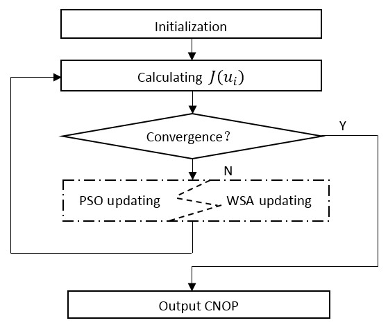
In Fig. 1, the most important part of the ACPW algorithm is inside the dotted box. We divide the entire initial swarm into two sub-swarms with the same number of individuals; one updates the individuals with the PSO's rule and the other with the WSA's rule. Then, the two sub-swarms are adaptively varied along with the convergence state of the ACPW algorithm. When the change in the objective function adaptive value is less than a threshold value, the number of individuals in the sub-swarm belonging to the WSA is increased and the other sub-swarm belonging to PSO is decreased by an equal number of individuals to keep the same number for the entire swarm. A more specific analysis of the ACPW algorithm is discussed in Sect. 4.

Table 1 The parameters of the ACPW.

The process of solving CNOPs with the ACPW algorithm is described as follows:

1. Randomly generate an initial swarm with N individuals. An individual u_i needs to satisfy the boundary constraint in the terms of Eq. (4). Once u_i goes beyond the boundary, it must be pulled back, i.e.,

   $$\begin{array}{}\text{(4)}& u_i=\left\{\begin{array}{l}{u}_i∥u_i∥\le \mathit{\delta },\\ {\displaystyle \frac{\mathit{\delta }}{∥u_i∥}}\times u_i∥u_i∥>\mathit{\delta },\end{array}\right.i=\mathrm{1},\mathrm{\cdots },N.\end{array}$$

   Divide the entire initial swarm into two sub-swarms with an adaptive coefficient α. One sub-swarm updates individuals with the PSO's rule and the other with the WSA's rule.

2. Calculate the adaptive value of the objective function in parallel, i.e.,= J(u_i) in Eq. (1).

3. Update individuals by the PSO (Eq. 5) or the WSA (Eq. 6). When

   $$\begin{array}{}\text{(5)}& \left\{\begin{array}{l}{v}_i^{k+\mathrm{1}}=\mathit{\omega }{v}_i^k+c_{\mathrm{1}}\mathit{\alpha }\left(o_i^k-u_i^k\right)+c_{\mathrm{2}}\mathit{\beta }\left(o_{\mathrm{g}}^k-u_i^k\right),\\ u_i^{k+\mathrm{1}}=u_i^k+\mathit{\gamma }{v}_i^{k+\mathrm{1}},\end{array}\right.\end{array}$$

   the superscript k or k+1 is the iterative step, $v_i^{k+\mathrm{1}}$ is the velocity of the individual $u_i^k$ calculated by the first sub-formula, ω is the inertia coefficient, c₁ and c₂ are the learning factors, α and β are the random numbers uniformly distributed on the interval from 0 to 1, $o_i^k$ is the local optimum, $o_{\mathrm{g}}^k$ is the global optimum in the kth iteration, γ is the restraint factor to control the speed and $u_i^{k+\mathrm{1}}$ is the updated individual based on PSO.

   There are two ways for updating individuals in the WSA, prey and escape, which represent the functions of searching in a local region and escaping from a local optimum. These are represented as

   $$\begin{array}{}\text{(6)}& \left\{\begin{array}{l}{u}_i^{k+\mathrm{1}}=u_i^k+\mathit{\theta }\cdot r\cdot \mathrm{rand}\left(\right)\mathrm{Prey},\\ u_i^{k+\mathrm{1}}=u_i^k+\mathit{\theta }\cdot s\cdot \mathrm{escape}\left(\right)\mathrm{Escape},\end{array}\right.\end{array}$$

   where the superscript k or k+1 is also the iterative step, θ is the velocity, r is the local optimizing radius that is smaller than the global constraint radius δ, rand(  ) is the random function whose mean value is distributed in $[-\mathrm{1},\mathrm{1}]$, escape(  ) is the function for calculating a random position that is 3 times larger than r and s is the step size of the updating individual.

   As described in Eq. (6), the wolf has two behaviors, i.e., prey and escape. The prey behavior uses the first sub-formula, and the second one is for the escape function that happens in every iteration when the condition p>p_a is satisfied, where p is a random number in [0,1] and p_a is the probability of an individual escaping from the current position.

4. Judge whether the change in the adaptive value of the objective function is smaller than ε. If so, set a new value for the adaptive sub-swarm coefficient α. If not, continue running the process. The detailed updating procedure for α is described as

   $$\begin{array}{}\text{(7)}& \mathit{\alpha }=\left\{\begin{array}{l}\mathit{\alpha }+\mathrm{0.05},\mathrm{if}\mathrm{the}\mathrm{bestvalue}-\mathrm{current}\mathrm{value}<\mathit{\epsilon },\\ \mathit{\alpha }-\mathrm{0.05},\mathrm{else}.\end{array}\right.\end{array}$$

   In this paper, before we update the individuals, α is calculated and we divide the entire initial swarm into two sub-swarms according to the α value i.e., the number of individuals depending on the PSO's rule is α×N and the other number is $(\mathrm{1}-\mathit{\alpha })\times N$. We set the initial value of ε and α to 0.1 and 0.5, respectively.

5. Judge whether the termination condition is satisfied. If so, terminate the iteration. Otherwise, go to step 2.

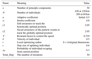
All of the above processes are based on the dimension reduction within the PCA, a procedure that has been described in the study of Mu et al. (2015a). After many experiments, the parameters of the ACPW algorithm can be set, as shown in Table 1.

Although there are more parameters than demanded for each single algorithm, most retain the empirical value of each algorithm and do not require adjustments. The reason for using a different number of individuals is that the internal storage memory was not sufficient when using more than 200 individuals, resulting in the premature termination of the ACPW algorithm.

3 Experiment design

All the experiments are run on a Lenove Thinkserver RD430 with two Intel Xeon E5-2450 2.10 GHz CPUs, 32 logical cores and 132G RAM. The operating system is CentOS 6.5. All the codes are written in the FORTRAN language and compiled by the PGI Compiler 10.2.

3.1 The model and data

In this paper, we adopt the MM5 model to study the sensitive region identification of TCAOs and the corresponding adjoint system of the MM5 model (Zou et al., 1997) is used to obtain the benchmark. The ERA interim daily analysis data (1^∘ × 1^∘) (Dee et al., 2011) from the European Centre for Medium range Weather Forecasts (ECMWF) are used to generate the initial and boundary conditions. The physical parameterization schemes are defined as dry convective adjustment, the high-resolution planetary boundary-layer scheme, grid-resolved large-scale precipitation, and the Kuo cumulus parameterization scheme.

We also utilize the best TC-track data (Ying et al., 2014) from the China Meteorological Administration–Shanghai Typhoon Institute (CMA–SHTI) as TC tracks observed for evaluating the simulation TC tracks of the MM5 model.

3.2 Typhoons Fitow (2013) and Matmo (2014)

TCs Fitow (2013) and Matom (2014) are taken as the study cases and introduced below. Fitow was the 23rd TC in 2013 and developed to the east of the Philippines on 29 September, striking China at Fuding in Fujian Province on 6 October. Matom was the 10th named typhoon in 2014. It formed on 17 July and reached land in Taiwan on 22 July. In these two cases, 24 h control forecasts are set as background fields based on integration from 00:00 UTC 5 October 2013 to 00:00 UTC 6 October 2013 (TC Fitow) and from 18:00 UTC 21 July 2014 to 18:00 UTC 22 July 2014 (TC Matom). After the 24 h period, TC Fitow had a maximum sustained wind of 162 km h⁻¹ whereas TC Matmo had a maximum wind speed of 151.2 km h⁻¹. In addition, the forecasts were executed at the 60 km and 120 km resolutions with 11 vertical levels, and the model domain covered 55 × 55 and 21 × 26 grids, respectively.

The simulated TC tracks from the MM5 model for these two cases are acceptable, as has been shown in our previous study (Zhang et al., 2017). The following analysis is based on those simulations.

3.3 Experimental setup

Because slight changes in the verification area never hurts the results (Zhou and Mu, 2011), we design the verification areas as rectangles covering the potential typhoon tracks at the forecast time.

The initial perturbation sample δu₀ is composed of the perturbed zonal wind u₀^′, meridional wind v₀^′, temperature ${T^{\prime }}_{\mathrm{0}}$ and surface pressure ${p^{\prime }}_{{\mathrm{s}}_{\mathrm{0}}}$. Each component can be represented as a matrix $am\times n\times l$, where m×n is the distribution of the horizontal grid, and l denotes the number of vertical levels. To extract features for reducing the dimensions and solving CNOPs, the $m\times n\times l$ matrix is reshaped to a k×1 vector, where $k=m\times n\times l\times S$ (S is the number of the components). Assuming we have R vectors to represent the features of the solution space, we recombine the R vectors to a k×R matrix and use the PCA to capture the feature space with lower dimensions. Then, the CNOP is solved in the space of the feature until we obtain the global CNOP, which will be projected to the original solution space. When using the ACPW algorithm to solve CNOPs, its initial inputs are produced randomly in the feature space, and the CNOP has the largest nonlinear evolution at the prediction time, i.e., the largest adaptive value of the objective function in Eq. (9). The objective function is measured by the total dry energy (Zhou and Zhang, 2014) since it has been proven that the sensitive regions gained by the dry energy are more beneficial than those obtained from the moist energy (Zhou, 2009).

The following is defined as

$$\begin{array}{}\text{(8)}& {\displaystyle }f\left(i,j\right)=\underset{\mathrm{0}}{\overset{\mathrm{1}}{\int }}{E}_{\mathrm{T}}(i,j,\mathit{\sigma })d\mathit{\sigma },\end{array}$$

where $E_{\mathrm{T}}\left(i,j,\mathit{\sigma }\right)$ denotes the total dry energy of the CNOP at the MM5 grid point $\left(i,j,\mathit{\sigma }\right)$.

Corresponding to Formulas (1) and (2), we have

$$\begin{array}{ll}{\displaystyle }\left(u_{\mathrm{NT}}\right)& {\displaystyle }={\displaystyle \frac{\mathrm{1}}{D}}\underset{D}{\int }\underset{\mathrm{0}}{\overset{\mathrm{1}}{\int }}\left[u_{\mathrm{t}}^{{}^{\prime }\mathrm{2}}+v_{\mathrm{t}}^{{}^{\prime }\mathrm{2}}+{\displaystyle \frac{c_{\mathrm{p}}}{T_{\mathrm{r}}}}{T}_{\mathrm{t}}^{{}^{\prime }\mathrm{2}}+R_{\mathrm{a}}{T}_{\mathrm{r}}{\left({\displaystyle \frac{p_{\mathrm{st}}^{\prime }}{p_{\mathrm{r}}}}\right)}^{\mathrm{2}}\right]\\ \text{(9)}& {\displaystyle }& {\displaystyle }\cdot d\mathit{\sigma }dD,\end{array}$$

where ${u^{\prime }}_{\mathrm{t}}$, $v_{\mathrm{t}{}^{\prime }}$, ${T^{\prime }}_{\mathrm{t}}$ and $p{{}^{\prime }}_{\mathrm{st}}$ are the components of u_NT, which is the nonlinear development of the perturbed U₀ (i.e., U₀+δu₀) from the initial time t₀ to the prediction time t, and σ is the vertical coordinate. Table 2 illustrates the other reference parameters.

For the convenience of optimization, solving CNOPs can be transformed into a minimized problem as

$$\begin{array}{ll}{\displaystyle }J\left(\mathit{\delta }{u}_{\mathrm{0}}^{\ast }\right)& {\displaystyle }=\left(-{\displaystyle \frac{\mathrm{1}}{D}}\underset{D}{\int }\underset{\mathrm{0}}{\overset{\mathrm{1}}{\int }}\left[{u^{\prime }}_{\mathrm{t}}^{\mathrm{2}}+{v^{\prime }}_{\mathrm{t}}^{\mathrm{2}}+{\displaystyle \frac{c_{\mathrm{p}}}{T_{\mathrm{r}}}}{T^{\prime }}_{\mathrm{t}}^{\mathrm{2}}+R_{\mathrm{a}}{T}_{\mathrm{r}}{\left({\displaystyle \frac{p_{\mathrm{st}}^{\prime }}{p_{\mathrm{r}}}}\right)}^{\mathrm{2}}\right]\right.\\ \text{(10)}& {\displaystyle }& {\displaystyle }\left.\cdot d\mathit{\sigma }dD\right).\end{array}$$

To facilitate understanding, all symbols are listed in Table 2, and their meanings are explained.

Table 2 The meanings of all symbols.

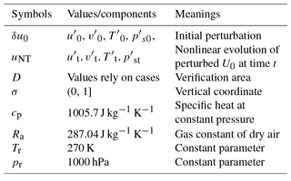
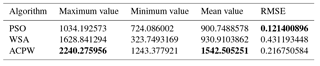
Table 3 The analysis results of the PSO, WSA and ACPW methods. The bold numbers represent the best values.

4 Experimental results and analysis

To evaluate the advantages of the ACPW algorithm, we run the PSO, WSA and ACPW programs 10 times and then compare the maximum, minimum and mean objective values as well as the RMSE. We also exhibit the objective value scope after the first iteration to analyze the effect of initial objective values on the different algorithms. Meanwhile, to illustrate the performance of the algorithms, we compare the degree of change of the objective function value for the three algorithms.

4.1 The advantages of the ACPW algorithm

Because the statistical analysis results are similar for the two TCs with two resolutions, we only describe the analysis of Fitow at a resolution of 60 km. Table 3 presents the maximum objective value, the minimum objective value, the mean objective value and the RMSE of the 10 results.

In Table 3, the maximum objective value is gained from the ACPW algorithm, and its mean value is also more than the other two algorithms. However, the RMSE of the PSO is the smallest, which shows the most stability.

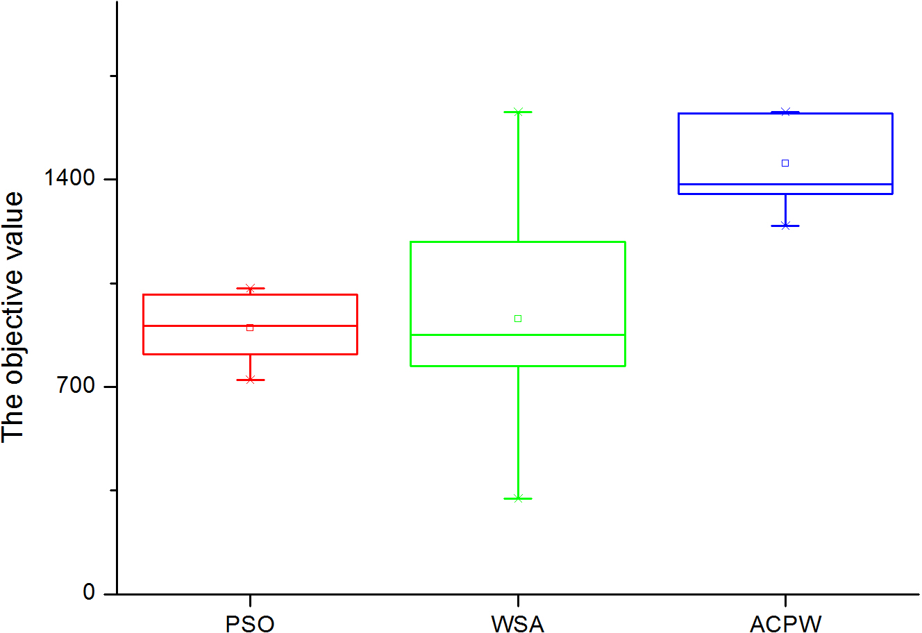
Figure 2 Box plot of the PSO, WSA and ACPW methods for TC Fitow at the 60 km resolution. The red box denotes PSO, the green box is for the WSA, and the blue box shows the results of the ACPW algorithm.

For additional analysis, we draw a box plot of the 10 results for the PSO, WSA and ACPW algorithms, as shown in Fig. 2. PSO has the narrowest range of values, although the objective values are smaller than the other two algorithms. The WSA has the widest range of values, although the objective values are also smaller than the ACPW algorithm. The ACPW algorithm has the second best stability, although it has the best objective values. The experiments display the stability of the PSO and the exploitation of the WSA. We combine the advantages of the PSO and WSA methods and use them to develop the ACPW algorithm to solve CNOPs. The analysis results demonstrate that the hybrid strategy and cooperative coevolution is both useful and effective.

Since these three algorithms are all heuristic algorithms generated randomly and the initial inputs are also generated by random way, the initial objective value is different for every run. To analyze the effect of initial objective values on the different algorithms, we exhibit the objective value scope of the PSO, WSA and ACPW algorithms after the first iteration in Fig. 3.

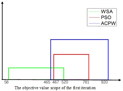
Figure 3 The first objective value scope of the PSO, WSA and ACPW methods. PSO is denoted as the red line, the WSA is shown as the green line and the ACPW algorithm is represented as the blue line.

In Fig. 3, for convenience, only the integer is indicated in the coordinate system. In 10 experiments, the PSO has the narrowest scope, from 467.1719 to 781.6482. The WSA and ACPW algorithms have similar value spans that are wider than the PSO, but the objective values of the ACPW are higher. And the value scope is reasonable according to the characteristics of these three algorithms. The WSA is the most random, the PSO is the most stable and the ACPW combines the advantages of the two. From the results, we cannot find the direct relationship between the initial objective value and the final results, but a better first objective value is beneficial in finding the optimal value.

To illustrate the improved performance of the ACPW algorithm, we calculate the average objective value of every step in 10 program results and obtain the change degree between the two iterations. We draw them in Fig. 4. If the objective value is continuously changing, then the algorithm has better global searching ability. Otherwise, the algorithm tends to experience a drop in local optimization.

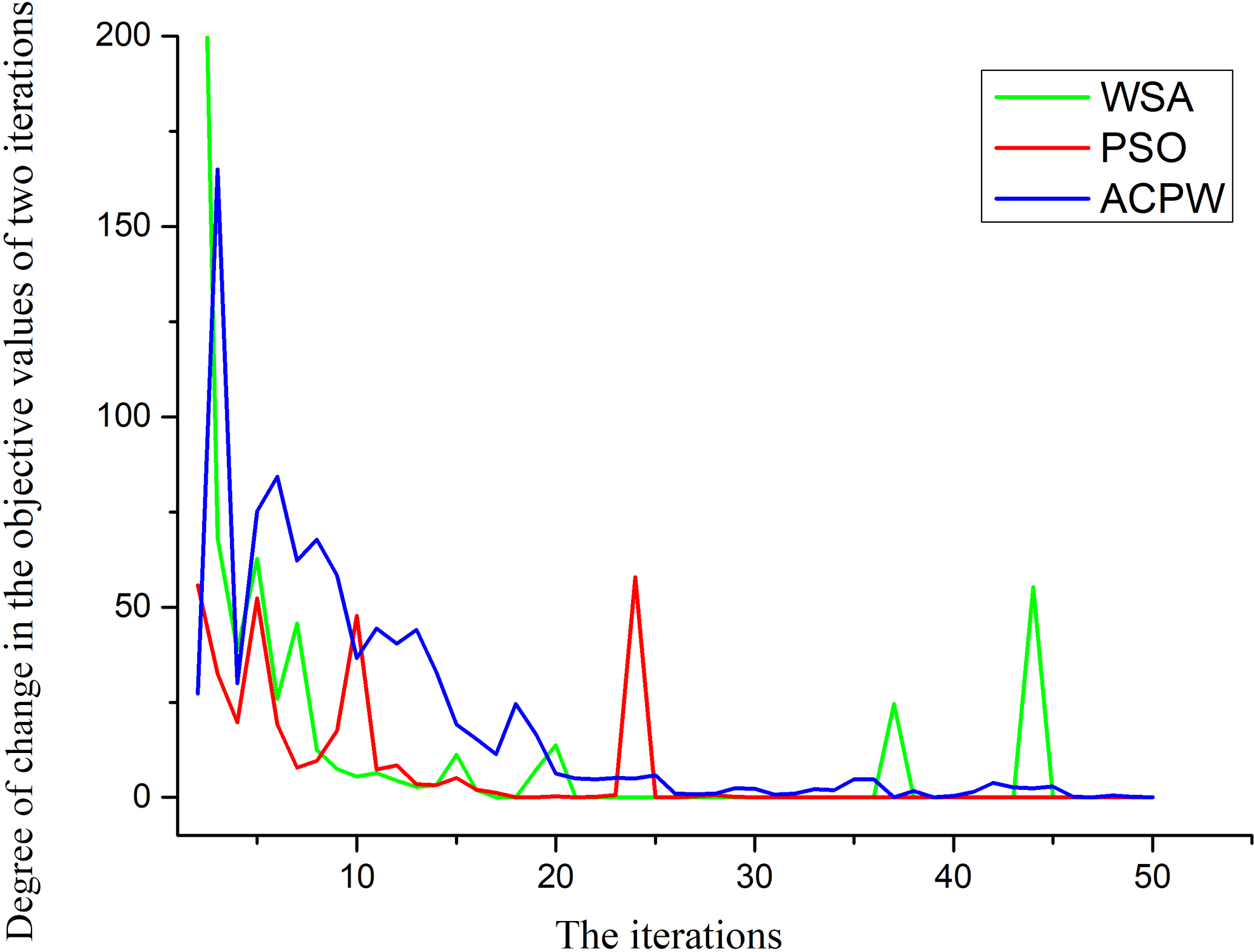
Figure 4 The degree of change of the PSO, WSA and ACPW methods. PSO is denoted as the red line, the WSA is shown as the green line and the ACPW algorithm is represented as the blue line.

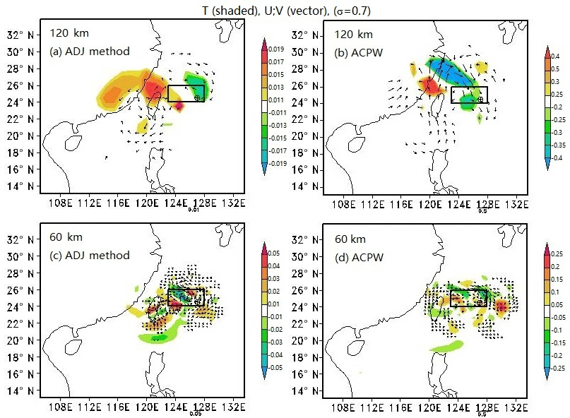
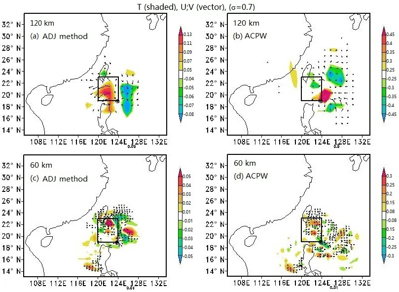
Figure 5 CNOP patterns at σ=0.7 for TC Fitow. The shaded parts represent temperature (units: K), and the vectors describe the wind (units: m s⁻¹). The squares indicate the verification areas, and the initial cyclone positions are shown by ⊕. Letters (a) and (b) denote the CNOP patterns at the 120 km resolution for the ADJ method and the ACPW algorithm, respectively, while letters (c) and (d) represent the CNOP patterns at the 60 km resolution for the ADJ method and the ACPW algorithm, respectively.

Figure 6 As described in Fig. 5 for tropical storm Matmo.

In Fig. 4, the degree of change is calculated from the subtraction of two objective values. For example, the objective value of the second iteration minus the first objective value is the first degree of change m has better performance than the PSO and WSA, because we combine their strengths using hybrid strategy and cooperative coevolution.

Figure 7 As described in Fig. 5, except where the shaded parts represent the vertically integrated energies (units: J kg⁻¹).

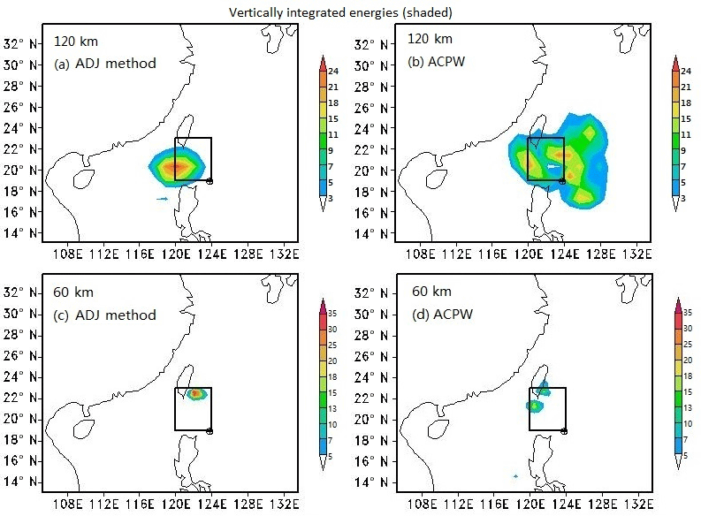
Figure 8 As described in Fig. 6, except where the shaded parts represent the vertically integrated energies (units: J kg⁻¹).

4.2 CNOP patterns

To validate the ACPW algorithm for solving CNOPs and to identify the sensitive regions, we compare the ADJ method and the ACPW algorithm results in terms of the CNOP patterns, energies, similarities, benefits from reduction of the CNOPs and simulated TC tracks with perturbations.

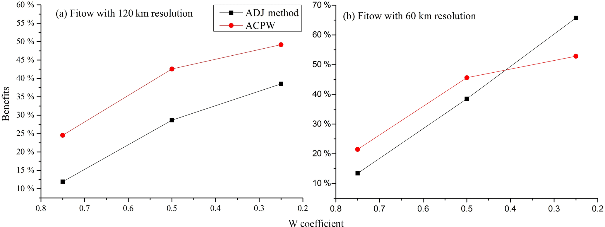
Figure 9 Benefits (in %) gained from reducing the CNOPs to W × CNOPs for the ADJ method and the ACPW algorithm across the entire domain for TC Fitow (2013). The x coordinate represents the W coefficient values, and the y coordinate denotes the benefits (in %) derived from the two methods. The ADJ method is presented as the black line with squares, and the ACPW result is the red line with circles.

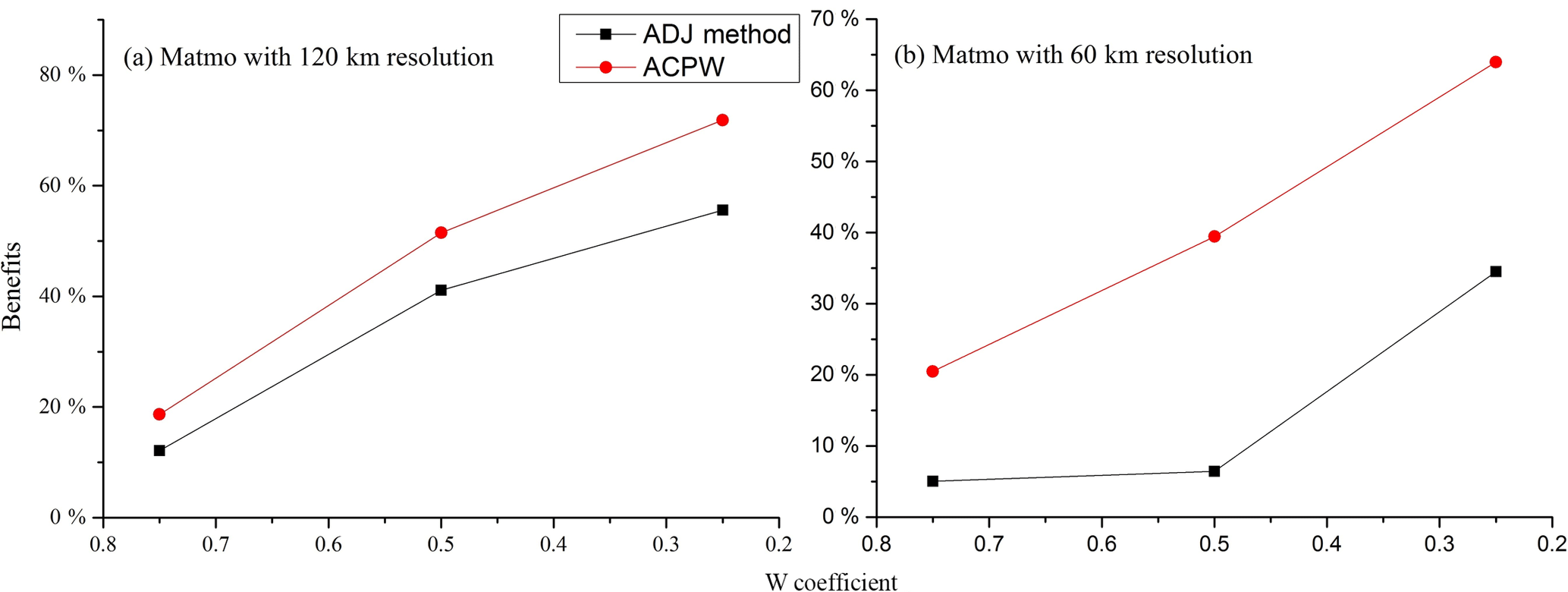
Figure 10 Benefits (in %) gained by reducing the CNOPs to W × CNOPs for the ADJ method and the ACPW algorithm across the entire domain for TC Matmo (2014). The x coordinate is the W coefficient values, and the y coordinate denotes the benefits (in %) derived from the two methods. The ADJ method is presented as the black line with squares, and the ACPW result is the red line with circles.

In this subsection, we compare the CNOPs obtained from the ADJ method and the ACPW algorithm in terms of the patterns of temperature and wind. Experimental results show that TC Fitow has more similar CNOP patterns than TC Matmo. The CNOP patterns are described in Fig. 5.

At the 120 km resolution for TC Fitow (Fig. 5a, b), the two methods have nearly the same major warm locations and similar cold regions, while the wind vectors have opposite directions. The ADJ method captures the CNOP with two major locations. The red (warm) location is distributed to the west of the initial cyclone (IC), while the green (cold) location is distributed to the north of the IC. The ACPW algorithm also captures the CNOP with two main locations. The warm one is distributed to the west and the cold one is located to the northwest of the IC. In this subsection, the spatial orientation is relative to the position of the IC. Therefore, in the following discussion, we explain the spatial orientation in the figures without repeating the IC.

For the TC Fitow analysis with a 60 km resolution (Fig. 5c, d), the CNOP spatial distribution based on the ACPW algorithm is very similar to the ADJ method's results. In the northwest of the verification area, the two CNOPs have two similar major parts, a warm area and a cold area. The difference between these two patterns is that the ADJ method has another major warm area located in the northwest, while the ACPW method produces another major warm area in the east. The distribution of the secondary parts exhibits only a slight difference.

For the same method with different resolutions (Fig. 5a, c and b, d), the CNOP patterns have similar major distributions in the northwest, although these occur within a different region. The reason is that when using a higher resolution, more small-scale phenomena can be resolved (Zhou and Mu, 2012a).

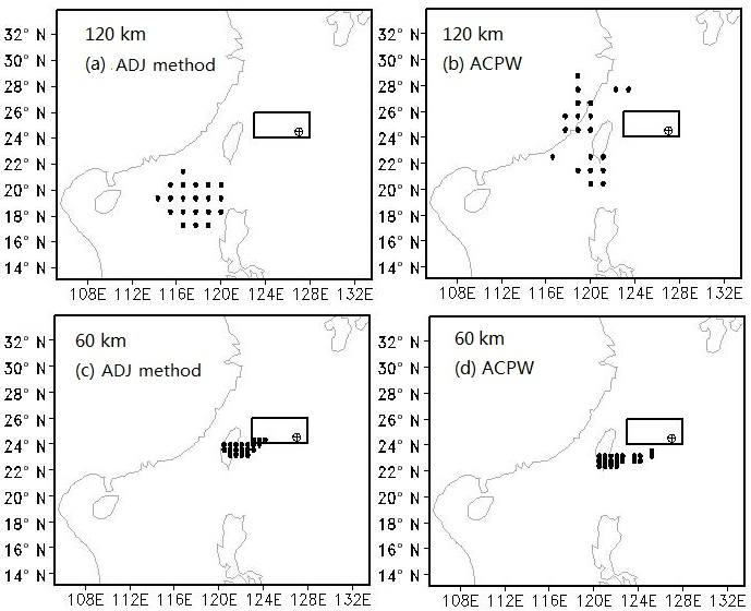
Figure 11 Sensitive regions identified by the CNOPs with 20 points for TC Fitow. The squares indicate the verification areas, and the initial cyclone positions are shown as ⊕. Letters (a) and (b) denote the CNOP patterns at the 120 km resolution for the ADJ method and the ACPW algorithm, respectively, while letters (c) and (d) represent the CNOP patterns at the 60 km resolution for the ADJ method and the ACPW algorithm, respectively.

Figure 12 Sensitive regions identified by the CNOPs with 20 points for TC Matmo. The squares indicate the verification areas, and the initial cyclone positions are shown as ⊕. Letters (a) and (b) denote the CNOP patterns at the 120 km resolution for the ADJ method and the ACPW algorithm, respectively, while letters (c) and (d) represent the CNOP patterns at the 60 km resolution for the ADJ method and the ACPW algorithm, respectively.

For the analysis of TC Matmo with a 120 km resolution (Fig. 6a, b), the ADJ method and the ACPW algorithm obtain CNOPs with different spatial patterns in terms of temperature and wind. The ADJ method has two major parts, with the warm part located in the west and the cold one in the east. The ACPW algorithm results in two main parts distributed in the northeast, with a warm area near the IC and a cold one far from the IC. For the analysis of TC Matmo with a 60 km resolution (Fig. 6c, d), in the verification area, the two CNOP patterns have similar spatial distributions, with two warm areas located at nearly the same positions. However, the parts outside the verification area are distributed in different locations. Moreover, the CNOP of the ADJ method has more regular distributions than the ACPW's distributions. For the same method with a different resolution (Fig. 6a, c and b, d), the CNOP patterns cover similar areas but with different ranges and details.

Based on the above analysis regarding the patterns of temperature and wind, we can conclude that when using a resolution of 60 km, the CNOPs predicted by the ADJ method and the ACPW algorithm have more similar major patterns than those predicted at a resolution of 120 km. In addition, the ACPW algorithm can obtain CNOPs with more similar patterns in TC Fitow than in TC Matmo.

The vertically integrated energies of the CNOPs for TC Fitow are displayed in Fig. 7. Compared to the ADJ method, at the 120 km resolution, the CNOPs of the ACPW method have much lower energy and differing positions. However, when using a resolution of 60 km, similar energies and positions are obtained. Moreover, the energy of the CNOPs obtained from the ACPW algorithm has a larger range in the center.

Vertically integrated energies of the CNOPs for TC Matmo are displayed in Fig. 8. Compared with the ADJ method, at the 120 km resolution, the CNOPs of the ACPW algorithm have a lower energy and cover larger areas. However, when using a resolution of 60 km, although the energy is still lower, the positions are more similar.

4.3 Similarities

When we evaluate the CNOPs, in addition to the characteristics and distributions of the CNOP patterns, consideration should also be given to the numerical similarities and the benefits of the CNOPs. Therefore, we calculate the similarity between the CNOPs determined from the ADJ method and the ACPW algorithm and use X and Y to represent them in the following formula, in which

$$\begin{array}{}\text{(11)}& {\displaystyle }{\mathrm{S}}_{\mathrm{xy}}={\displaystyle \frac{\langle X,Y\rangle }{\sqrt{\langle X,X\rangle }\sqrt{\langle Y,Y\rangle }}}.\end{array}$$

The results are shown in Table 4. The similarity values can reflect the similarities among the CNOP patterns (Figs. 5 and 6).

Table 4 The similarities of CNOPs gained from the ACPW and ADJ method.

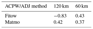
In Table 4, for TC Fitow, the similarity at 120 km is −0.83, whereas the similarity with a resolution of 60 km is 0.43. For the analysis of TC Matmo, the similarity at 120 km is 0.42, whereas that with a resolution of 60 km is 0.37. The negative sign indicates that portions of the CNOPs from these two methods have opposite wind–vector directions, which is shown in Fig. 5. We also find that when using a higher resolution, the similarity is lower. The reason for this finding is that although the major patterns of the CNOPs are similar, the secondary parts differ and they cover larger areas. When using a higher resolution, we can achieve information on a smaller scale, and the identification of sensitive regions becomes more accurate. Regarding the analysis of the CNOP patterns, we obtain more similar major patterns when for a resolution of 60 km. However, compared with the different parts, the similar parts are very small. The similarities decreased do not affect the identification of the sensitive regions because the adaptive observations only focus on the points with larger influences, which will be demonstrated Sect. 4.4.

Table 5 The ratios of energy for 24 h evolution through the insertion of the CNOPs from the ACPW algorithm and ADJ method into the initial states.

We also compare the energy for 24 h of nonlinear development under the initial states perturbed by different CNOPs, i.e., $J\left(M\right({\mathit{U}}_{\mathrm{0}}+\mathit{\delta }{u}_{\mathrm{0}}^{\ast }\left)\right)$. The results are shown in Table 5. All CNOPs obtained using the ACPW produce lower energies than the those of the ADJ method. However, when reducing the CNOPs to W×CNOPs in the entire domain and reducing the CNOPs by a factor of 0.5 in the sensitive regions, the ACPW algorithm has better results, which will be discussed in following subsection.

4.4 Benefits from reducing the CNOPs

In this subsection, we design two groups of idealized experiments to investigate the validity of the sensitive regions identified using CNOPs based on two assumptions.

First, when adding adaptive observations in sensitive regions, the surrounding environment is idealized, and the improvements from adding observations reduce the original errors by a factor of 0.5.

Second, the obtained CNOPs can be seen as the optimal initial perturbations. Once we reduce them in the sensitive regions, the benefits are the highest.

Under these assumptions, by reducing the CNOPs to W×CNOPs and inserting them into the initial states, we can investigate how the reductions in the CNOPs influence the skill of TC forecasting. Moreover, reducing the CNOPs by a factor of 0.5 in the identified sensitive regions by vertically integrating the energies can be used investigate how the addition of adaptive observations in the sensitive regions can impact the skill of TC forecasting.

First, because CNOPs can be seen as the optimal initial perturbations in the TCAOs, we reduce the CNOPs to W×CNOPs, where W is a coefficient in (0, 1), insert the reduced CNOPs into the initial state and allow for 24 h of evolution of the MM5 model. Then, we calculate the forecast error using Formula (14) to determine the benefits of the reductions. Second, we determine the sensitive regions via vertically integrated energies using two schemes, namely the same points in the different resolutions and the equivalent percentage of points from the different grids. Then, we reduce the CNOPs by a factor of 0.5 in only the sensitive regions and insert the amended CNOPs into the initial states. The model is run for 24 h. The experimental results are described below.

4.4.1 Reducing the CNOPs to W × CNOPs in the entire domain

We explore the forecast improvements induced by reducing the CNOPs to W × CNOPs for the entire domain. The approach requires using the reduced CNOPs in their initial state for a 24 h simulation of the MM5 model. The prediction error is computed by Formula (12), where

$$\begin{array}{}\text{(12)}& {\displaystyle }{J}_{\mathrm{1}}\left(u_{\mathrm{NT}}\right)={∥PM\left(U_{\mathrm{0}}+\mathit{\delta }{u}_{\mathrm{0}}\right)-PM\left(U_{\mathrm{0}}\right)∥}^{\mathrm{2}},\end{array}$$

and the definitions of u_NT, P, M and U₀ are the same as in Eqs. (1), (2), and (3).

Figure 13 Sensitive regions identified by the CNOPs with 6 points at the 120 km resolution and 30 points at the 60 km resolution for TC Fitow. The squares indicate the verification areas, and the initial cyclone positions are shown as ⊕. The letters (a) and (b) denote the CNOP patterns at the 120 km resolution for the ADJ method and the ACPW algorithm, respectively, while letters (c) and (d) represent the CNOP patterns at the 60 km resolution for the ADJ method and the ACPW algorithm, respectively.

Figure 14 Sensitive regions identified by the CNOPs with 6 points at the 120 km resolution and 30 points at the 60 km resolution for TC Fitow. The squares indicate the verification areas, and the initial cyclone positions are shown as ⊕. Letters (a) and (b) denote the CNOP patterns at the 120 km resolution for the ADJ method and the ACPW algorithm, respectively, while letters (c) and (d) represent the CNOP patterns at the 60 km resolution for the ADJ method and the ACPW algorithm, respectively.

The prediction error after reducing the CNOPs for the entire domain is computed by Formula (13), where

$$\begin{array}{}\text{(13)}& {\displaystyle }{J}_{\mathrm{2}}\left(u_{\mathrm{NT}}\right)={∥PM\left(U_{\mathrm{0}}+W\mathit{\delta }{u}_{\mathrm{0}}\right)-PM\left(U_{\mathrm{0}}\right)∥}^{\mathrm{2}},\end{array}$$

and W is the weighting coefficient, which is set to 0.25, 0.5 or 0.75 for decreasing error. The benefit from such reductions is calculated by Formula (14), represented as

$$\begin{array}{}\text{(14)}& {\displaystyle \frac{J_{\mathrm{1}}\left(u_{\mathrm{NT}}\right)-J_{\mathrm{2}}\left(u_{\mathrm{NT}}\right)}{J_{\mathrm{1}}\left(u_{\mathrm{NT}}\right)}}.\end{array}$$

The prediction benefit increases for decreasing W. Figures 9 and 10 also show that the ACPW algorithm can obtain CNOPs with better benefits from reducing the CNOPs to W×CNOPs for the entire domain than the ADJ method except for when W is 0.25 for TC Fitow at a resolution of 60 km. This is because the ACPW algorithm optimizes a low-dimensional feature space due to the PCA and focuses on more effective points in the entire domain, which has positive effects on improving the forecast.

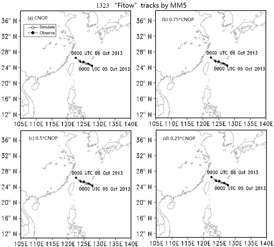
Figure 15 Simulated TC tracks from MM5 through the insertion of the CNOPs or W × CNOP into the initial state in the entire domain for TC Fitow. Solid circles represent the observed TC tracks from the CMA, and the hollow circles show the simulated TC tracks from the MM5 model. Letters (a), (b), (c) and (d) denote the CNOP, 0.75 × CNOP, 0.5 × CNOP and 0.25 × CNOP results, respectively.

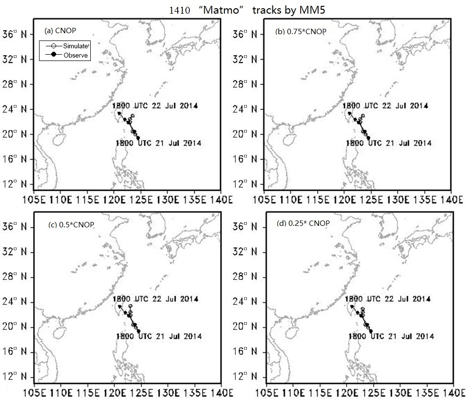
Figure 16 Simulated TC tracks from MM5 through the insertion of the CNOPs or W × CNOP into the initial state in the entire domain for TC Matmo.

4.4.2 Reducing the CNOPs by a factor of 0.5 in the sensitive regions

We explore the forecast improvement caused by reducing the CNOPs by a factor of 0.5 in the sensitive regions. We determine the sensitive regions based on vertically integrated energies using two schemes, the 20 points with the highest energy at the different resolutions and 1∕100 points of the different grids, which is 30 points at the 60 km resolution (55 × 55) and 6 points at the 120 km resolution (21 × 26). The sensitive regions with the 20 points having the highest energy are denoted in Figs. 11 and 12.

In Figs. 11 and 12, when the equivalent points approach is adopted, a larger scope is covered with the 120 km resolution than with the 60 km resolution. When using the 20 points from the ADJ method and the ACPW algorithm and reducing the CNOPs by a factor of 0.5, the benefits are displayed in Table 6.

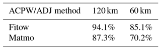
Table 6 Benefits (in %) gained from reducing the CNOPs by a factor of 0.5 in the sensitive regions identified by the ADJ method and the ACPW algorithm with 20 points. The bold numbers represent the best values of the ACPW.

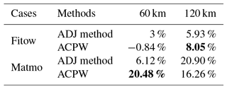
In Table 6, for TC Fitow, compared to the ADJ method, i.e., 5.93 % at the 120 km resolution and 3 % at the 60 km resolution, the ACPW algorithm obtains a higher benefit (8.05 %) for a resolution of 120 km and a lower benefit (−0.84) for a resolution of 60 km. Here, −0.84 % means that a reduction in the CNOPs results in no benefit and narrows the quality of the initial state. For the analysis of TC Matmo, the ACPW algorithm achieves a much higher benefit (20.48 %) than the ADJ method (6.12 %) at the 60 km resolution and a lower benefit (16.26 %) than the ADJ method (20.90 %) at the 120 km resolution. In addition, when using the same number of energy points, the benefits from using the 120 km resolution are nearly as high as those for the 60 km resolution except for the ACPW algorithm at 60 km resolution for TC Matmo.

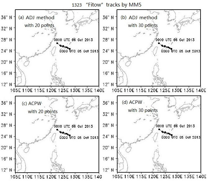
Figure 17 Simulated TC tracks from MM5 through the insertion of the amended CNOPs, which are reduced by a factor of 0.5 only in the sensitive regions, into the initial state for TC Fitow. Solid circles represent the observed TC tracks from the CMA, and the hollow circles show the simulated TC tracks from the MM5 model. (a), (b), (c) and (d) denote the ADJ method with 20 points, ADJ method with 30 points, ACPW algorithm with 20 points and the ACPW algorithm with 30 points, respectively.

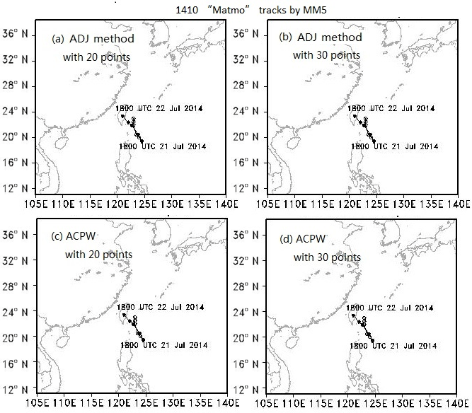
Figure 18 Simulated TC tracks from MM5 through the insertion of the amended CNOPs, which are reduced by a factor of 0.5 only in the sensitive regions, into the initial state for TC Matmo.

The sensitive regions with 1∕100 points from the different grids are denoted in Figs. 13 and 14.

Figures 13 and 14 show that when using different resolutions, the sensitive regions identified by the same method are different. The sensitive regions identified by the ACPW algorithm are more dispersive than those identified by the ADJ method, which is attributed to the randomness of the intelligent algorithms. Table 7 shows the benefits gained from reducing the CNOPs by a factor of 0.5 in the sensitive regions identified by the ADJ method and the ACPW algorithm with different points in the different resolutions.

Table 7 Benefits (in %) gained from reducing the CNOPs by a factor of 0.5 in the sensitive regions identified by the ADJ method and the ACPW algorithm with 6 points at the 120 km resolution and 30 points at the 60 km resolution. The bold numbers represent the best values of the ACPW.

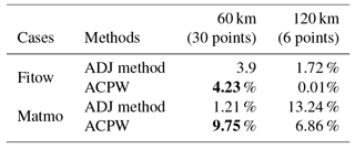
According to Table 7, for TC Fitow, the ACPW algorithm achieves a 4.23 % benefit, which is higher than the ADJ method (3.9 %) at the 60 km resolution and a lower benefit 0.01 % than the ADJ method (1.72 %) at the 120 km resolution. For the analysis of TC Matmo, the ACPW algorithm also has a higher benefit (9.75 %) and a lower benefit (6.86 %) than the ADJ method (1.21 % and 13.24 %, respectively).

Combined with Tables 6 and 7, we can conclude that the sensitive regions cover a larger scope and higher benefits are obtained. When using the same proportion of grids with the different resolutions, the sensitive regions under higher resolution achieve higher benefits. These results also demonstrate that the CNOPs obtained from the ACPW algorithm can identify sensitive regions with higher benefits at the 60 km resolution.

4.5 Simulated TC tracks

We further investigate the validity of the sensitive regions identified by the CNOPs through using a comparison of simulated TC tracks predicted by the MM5 model for each case by inserting the CNOPs or W × CNOPs into the initial states. We also simulate the TC tracks through the insertion of the amended CNOPs in the different sensitive regions (20 or 30 points). Because 120 km is the lowest resolution in this research and the tracks cannot be drawn under this resolution in our study, we only analyze the simulated TC tracks at the 60 km resolution. We draw two tracks in a sub-figure, which are represented by the observed TC tracks from the CMA–SHTI and the simulated TC track from the MM5 model, and the different perturbations are overlayed onto the same initial states. According to the experimental results, when overlaying the CNOPs or amended CNOPs onto the same initial states, although the CNOPs are obtained from different methods, the simulated tracks are the same. Therefore, we only discuss one group of figures for each case. The results are presented in Figs. 15 and 16.

Figure 15 demonstrates the simulated TC tracks of the MM5 by inserting the CNOPs or W × CNOP into the initial state for TC Fitow; the four sub-figures are the same. The reason is that the deviations of the simulated TC track and the observed TC track are very small. Therefore, it is not easy to make improvements. Hence, when inserting different CNOPs into identical initial states to simulate TC tracks, a change is not evident. Moreover, the resolution we used was 60 km, which is not high enough to show more details about changing tracks.

Figure 16 demonstrates the simulated TC tracks from the MM5 model by inserting the CNOPs or W × CNOP into the initial state for TC Matmo. Figure 16a and b are the same, and from Fig. 16b to d, the simulated positions after 24 h become closer to the observed positions. These results illustrate that when the CNOPs obtained by the ACPW algorithm and ADJ method are used as the optimal initial perturbations, reducing the CNOPs has a positive effect on the skill of the forecasting of the simulated tracks. Moreover, the ACPW algorithm is a meaningful and effective method for solving the approximate CNOPs of the ADJ method.

We also simulate TC tracks by inserting the amended CNOPs, which are reduced by a factor of 0.5 in only the sensitive regions. We use 20 and 30 points as the sensitive regions to study how the number of points affects the skill of forecasting. The results are shown in Figs. 17 and 18.

In Figs. 17 and 18, the simulated TC tracks are the same not only for different methods but also for different sensitive regions. We can conclude that the ACPW algorithm, an adjoint-free method, is a meaningful and effective method for solving the approximate CNOPs of the ADJ method. According to these results, we can also conclude that using 20 or 30 points as the sensitive regions results in the same improvement in the TC tracks in terms of forecasting. Thus, fewer points can be used in real adaptive observations to reduce costs.

4.6 The efficiency of the ACPW algorithm

To promote the efficiency of the ACPW algorithm, we parallelize it with MPI technology. The time consumption of each case is nearly the same. Hence, we can use a group of experimental results to elucidate the efficiency of the ACPW algorithm. Because the ADJ method cannot be parallelized because each input depends on the output of the previous step, its time consumption is not changed. Moreover, because this method generally uses 4 ∼ 8 initial guess fields to obtain the optimal value, we use 1 and 4 initial guess fields to determine the CNOPs. The time consumption of the ADJ method and the ACPW algorithm are shown in Table 8.

Table 8 The time consumption of the ADJ method and the ACPW algorithm (unit: min). The bold numbers represent that the ACPW has the minimum time consumption.

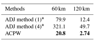
^* ADJ method (1) means using 1 initial guess field and ADJ method (4) means using 4 initial guess fields.

At the 120 km resolution, the time consumption of the ADJ method using 1 and 4 initial guess fields is 12.4 and 49.7 min, respectively. At the 60 km resolution, the time consumption is 79.9 and 321.1 min, respectively. Unlike the ADJ method, the ACPW algorithm can be parallelized. When using 22 cores, the ACPW method requires much less time, i.e., 2.74 min at the 120 km resolution and 20.8 min at the 60 km resolution. Obviously, the ACPW is more efficient. Compared to the ADJ method (1), the speedup reaches 4.53 and 3.84 for the different resolutions. Compared to the ADJ method (4), the speedup reaches 18.14 and 15.44. Although the different initial guess fields are calculated in parallel, the time consumption must be higher than that of the ADJ method (1), since the ACPW algorithm is also faster than the ADJ method.

5 Summaries and conclusions

In this study, we present a novel approach, the adaptive cooperative coevolution of the parallelized PSO and WSA (ACPW), to solve CNOPs. The CNOPs based on the ACPW algorithm are applied to study the identification of sensitive regions by TCAOs in the MM5 model without using an adjoint model. We study two TC cases, Fitow (2013) and Matmo (2014), with 60 and 120 km resolutions. The objective function is set as the total dry energy based on 24 h simulations starting with initial perturbations at the prediction time within the verification area. We also calculate CNOPs with the ADJ method, using results as a benchmark. To validate the ACPW algorithm, the CNOPs obtained from the different methods are compared in terms of the patterns, energies, similarities, benefits in reducing the CNOPs and simulated TC tracks with perturbations. To evaluate the advantages of the ACPW algorithm, we run the PSO, WSA and ACPW programs 10 times and compare the maximum, minimum and mean objective values as well as the RMSE. We also exhibit the objective value scope after the first iteration to analyze the effect of initial objective values on the different algorithms. To illustrate the performance of the algorithms, we compare the degree of change of the objective function value for the three algorithms. The analysis results demonstrate that the hybrid strategy and cooperative coevolution are useful and effective.

According to all of the experiments, the following five conclusions are obtained:

• 1.

  Compared with the ADJ method, the ACPW algorithm can obtain CNOPs with more similar patterns of temperature and wind for TC Fitow than those for TC Matmo.

• 2.

  At the 120 km resolution, the similarities in the CNOPs achieved by the ADJ method and the ACPW algorithm are higher than those at the 60 km. The reason is that although the major patterns of the CNOPs are similar, the other parts differ and cover larger areas. At a higher resolution, we can find information on a smaller scale. Moreover, sensitive region identification becomes more accurate. Regarding the CNOP patterns, more similar major patterns are obtained at the 60 km resolution, although the similar parts are very small compared with the other differing parts. However, the decreased similarities do not affect identifying sensitive regions because the adaptive observations only focus on the points with a larger influence.

• 3.

  When adding adaptive observations in the sensitive regions for a surrounding environment that is idealized, the original errors are reduced by a factor of 0.5. Thus, the CNOPs can be seen as the optimal initial perturbations. Once they are reduced in the sensitive regions, the benefits are highest. We design two groups of idealized experiments to investigate the validity of the sensitive regions identified by the CNOPs for the skill of TC-track forecasting. This involves reducing CNOPs to W × CNOPs and reducing the CNOPs by a factor of 0.5 in the sensitive regions identified using vertically integrated energies. The experimental results show that the CNOPs of the ACPW algorithm produce lower energies than the ADJ method but can obtain better benefits when reducing the CNOPs.

• 4.

  The ACPW algorithm can be effective for identifying the sensitive regions, which have the same influence on the forecast improvements of the simulated TC tracks as the ADJ method. We compare the different forecast improvements of the TC tracks with the different reduced perturbations, including reducing the CNOPs to W × CNOPs for the entire domain and reducing the CNOPs by a factor of 0.5 in the sensitive regions. The experimental results all support our conclusions.

• 5.

  The ACPW algorithm is more efficient than the ADJ method. Compared to the ADJ method using 1 initial guess field, the speedup reaches 4.53 at the 120 km resolution and 3.84 at the 60 km resolution. Compared to the ADJ method using 4 initial guess fields, the speedup reaches 18.14 and 15.44 for the 120 km and 60 km resolutions, respectively.

All of the conclusions demonstrate that the ACPW algorithm is a meaningful and effective method for solving approximate CNOPs and identifying the sensitive regions of TCAOs. In addition, as we reduce the dimensions within the PCA, the CNOPs lose some energy. Compared to the CNOPs form the ADJ method, the CNOPs from the ACPW algorithm are all local CNOPs. However, for the ACPW algorithm, they are global CNOPs. Because the PCA makes our optimization focus on more effective points with higher energies, the ACPW algorithm can achieve the CNOPs with better benefits and the same improvements in the skill of TC-track forecasting.

We are restricted to computation sources for the time being. We are also limited by the parallelization of the ACPW algorithm. We will improve the conditions of computation and use the parallel ACPW algorithm to solve CNOPs in the Weather Research and Forecasting (WRF) model with a finer grid and higher resolution. In addition, we will apply this type of method to solve CNOPs in the Community Earth System Model (CESM) model, which does not have an adjoint model.