The onset of chaos in nonautonomous dissipative dynamical systems: a low-order ocean-model case study

A four-dimensional nonlinear spectral ocean model is used to study the transition to chaos induced by periodic forcing in systems that are nonchaotic in the autonomous limit. The analysis relies on the construction of the system's pullback attractors (PBAs) through ensemble simulations, based on a large number of initial states in the remote past. A preliminary analysis of the autonomous system is carried out by investigating its bifurcation diagram, as well as by calculating a metric that measures the mean distance between two initially nearby trajectories, along with the system's entropy. We find that nonchaotic attractors can still exhibit sensitive dependence on initial data over some time interval; this apparent paradox is resolved by noting that the dependence only concerns the phase of the periodic trajectories, and that it disappears once the latter have converged onto the attractor. The periodically forced system, analyzed by the same methods, yields periodic or chaotic PBAs depending on the periodic forcing's amplitude ε. A new diagnostic method – based on the cross-correlation between two initially nearby trajectories – is proposed to characterize the transition between the two types of behavior. Transition to chaos is found to occur abruptly at a critical value ε_c and begins with the intermittent emergence of periodic oscillations with distinct phases. The same diagnostic method is finally shown to be a useful tool for autonomous and aperiodically forced systems as well.

1 Introduction and motivation

Understanding the mechanisms that lead to the onset of chaos in dissipative dynamical systems is of fundamental importance both from a cognitive viewpoint and for the correct use of the mathematical models on which the systems are based. Chaos arises in such systems as a control parameter in the governing equations crosses a given threshold. A huge amount of work has been devoted to analyzing the transition to chaos in the framework of autonomous dynamical systems, i.e., in systems in which the external forcing and the coefficients do not depend on time. The various routes to chaos in autonomous dissipative systems – in the presence of time-independent forcing — include period-doubling cascades, intermittency and crisis, quasiperiodic routes, and global bifurcations (e.g., Nicolis, 1995; Hilborn, 2000; Ott, 2002; Tél and Gruiz, 2006; Strogatz, 2015).

Nonautonomous dissipative dynamical systems represent a crucial extension of autonomous systems for practical applications, since the external forcing in most real systems – whether deterministic, random or both – depends, typically, on time. Despite their importance, nonautonomous systems have received, until recently, less attention than autonomous systems. Transition to chaos induced by time-dependent forcing has, nonetheless, been studied in several significant cases. A classical example is the Van der Pol oscillator (Van der Pol, 1920, 1926), in which chaotic relaxation oscillations emerge under the effect of an external periodic forcing. A few more recent examples in the climate sciences include (i) transition to chaos due to quasiperiodic forcing (Le Treut and Ghil, 1983; Ghil, 1994); (ii) modification of the autonomous transition by periodic forcing (Sushama et al., 2007); and (iii) the important contributions of Anna Trevisan and colleagues to the data assimilation problem for chaotic systems, in which the data stream can be seen essentially as a time-dependent forcing (Trevisan and Uboldi, 2004; Carrassi et al., 2008a, b; Trevisan and Palatella, 2011).

The onset of chaos is analyzed here in the framework of nonautonomous systems, which has been received rapidly increasing attention recently in the context of climate dynamics (Ghil et al., 2008; Chekroun et al., 2011; Bódai and Tél, 2012; Bódai et al., 2013; Pierini, 2014; Drótos et al., 2015, 2017; Ghil, 2015, 2017; Pierini et al., 2016; Lucarini et al., 2017). Our study focuses on a four-dimensional nonlinear spectral ocean model (Pierini, 2011), which is subjected to periodic forcing, chosen as the simplest form of time dependence. Cases will be considered that are nonchaotic in the autonomous limit, so that the chaos that emerges in the system is strictly associated with the nonstationarity of the forcing.

The study makes use of ensemble simulations performed with many initial states distributed in a given subset of phase space, following the methodology of Pierini (2014) and Pierini et al. (2016). The overall idea is that the relevant information in the climate system must be derived from statistical analyses of an ensemble of different system trajectories, each corresponding to a different initial state, provided that the corresponding trajectories have converged to the system's time-dependent attractor.

Such an attractor is called a pullback attractor (PBA; e.g., Ghil et al., 2008; Chekroun et al., 2011; Kloeden and Rasmussen, 2011; Carvalho et al., 2012) in the mathematical literature and a snapshot attractor (e.g., Romeiras et al., 1990; Bódai and Tél, 2012; Bódai et al., 2013) in the physical literature; it provides the natural extension to nonautonomous dissipative dynamical systems of the classical concept of an attractor that is fixed in time for autonomous systems. A global PBA is defined as a time-dependent set 𝒜(t) in the system's phase space that is invariant under its governing equations, along with the equally time-dependent, invariant measure μ(t) supported on this set, and to which all trajectories starting in the remote past converge (Arnold, 1998; Rasmussen, 2007; Kloeden and Rasmussen, 2011; Carvalho et al., 2012). In the deterministic case, it is understood that 𝒜(t) depends also on the particular forcing, say F(t), that is being applied, but this dependence is usually not kept track of in the notation. In the random case, the PBA is called a random attractor, and the dependence on the specific realization ω of the noise process is often included in the notation, as 𝒜(t,ω).

Pierini et al. (2016) rigourously proved that a weakly dissipative nonlinear model like the one used there and herein does possess a global PBA, subject to mild integrability conditions on the forcing. In the present study, the numerical approach used for the systematic investigation of the system's PBAs follows Pierini (2014) and Pierini et al. (2016). Further diagnostic tools will be introduced for the present periodic-forcing setup, and a new diagnostic tool will also be proposed to monitor the onset of chaos in our nonautonomous system.

The paper is organized as follows. In Sect. 2, the mathematical model is described. In Sect. 3, the main properties of the autonomous system are summarized and an apparent paradox related to the sensitivity to initial states in the periodic regime is discussed. In Sect. 4, the results obtained for the periodically forced system are presented and discussed; the new cross-correlation-based method specifically formulated to characterize the onset of chaos is introduced and applied to the specific case at hand. This method helps characterize the transition to chaos as the amplitude of the periodic forcing increases, as well as document the coexistence of local PBAs with chaotic and nonchaotic behavior within the model's global PBA. In Sect. 5, the same method is shown to be a useful tool also for autonomous and aperiodically forced systems. Finally, in Sect. 6 the results are summarized and conclusions are drawn. An appendix illustrates in greater detail the coexistence of local PBAs that are chaotic and nonchaotic in the setting of a periodically forced Van der Pol–Duffing oscillator.

2 Model description

The highly idealized model of the oceans' wind-driven, double-gyre circulation (Ghil, 2017, and references therein) used in the present study is governed by the system of four nonlinear, coupled ordinary differential equations derived by Pierini (2011); Vannitsem (2014), Vannitsem and De Cruz (2014) and De Cruz et al. (2018) used this model to represent the ocean component in their low-order climate models. The author introduced such a low-order model to complement the process studies on the Kuroshio Extension's low-frequency variability previously carried out with a much more detailed, primitive equation ocean model (e.g., Pierini, 2006; Pierini et al., 2009; Pierini and Dijkstra, 2009). The same low-order model was later used by Pierini (2014) and Pierini et al. (2016) to explore the PBAs of the system in various cases. Here we merely review the main aspects of the model; for all the technical details and parameter values, the interested reader should kindly refer to Pierini (2011).

The dynamics are governed by the evolution equation of potential vorticity in the quasigeostrophic approximation on the beta plane for a shallow layer of fluid, superimposed on an infinitely deep quiescent lower layer. Pierini (2006) found such a reduced-gravity model to be a good approximation for process studies of the Kuroshio Extension's low-frequency variability. The flow is described by the streamfunction ψ(x,t): like in the previous studies, ψ, the horizontal coordinates $\mathbf{x}=(x,y)$ and the time t are dimensionless, but the dimensional time will be plotted in all the time series presented in this study to emphasize the typical timescales of the oceanic phenomena under investigation.

A four-dimensional spectral model is obtained by expanding the streamfunction in a rectangular domain as follows:

$$\begin{array}{}\text{(1)}& \mathit{\psi }\left(\mathbf{x},t\right)=\sum _{i=\mathrm{1}}^{\mathrm{4}}{\mathrm{\Psi }}_i\left(t\right)\left|i\right.〉.\end{array}$$

The orthonormal basis |i〉 is defined as follows:

$$\begin{array}{ll}{\displaystyle }& {\displaystyle }\left|\mathrm{1}\right.〉=e^{-\mathit{\alpha }x}\sin x\sin y;\left|\mathrm{2}\right.〉=e^{-\mathit{\alpha }x}\sin x\sin \mathrm{2}y,\\ {\displaystyle }& {\displaystyle }\left|\mathrm{3}\right.〉=e^{-\mathit{\alpha }x}\sin \mathrm{2}x\sin y;\left|\mathrm{4}\right.〉=e^{-\mathit{\alpha }x}\sin \mathrm{2}x\sin \mathrm{2}y,\end{array}$$

where α is a real positive constant. This basis satisfies the free-slip boundary conditions along the borders of the rectangular domain; it also captures the oceanic flow's westward intensification thanks to the exponential factor first introduced in the two-dimensional model of Jiang et al. (1995).

The four nonlinear coupled ordinary differential equations that govern the evolution of the vector $\mathbf{\Psi }\left(t\right)=\left({\mathrm{\Psi }}_{\mathrm{1}},{\mathrm{\Psi }}_{\mathrm{2}},{\mathrm{\Psi }}_{\mathrm{3}},{\mathrm{\Psi }}_{\mathrm{4}}\right)$ can be written (see Pierini, 2011) as

$$\begin{array}{}\text{(2)}& {\displaystyle \frac{\mathrm{d}\mathbf{\Psi }}{\mathrm{d}t}}+\mathbf{\Psi }\mathbf{J}\mathbf{\Psi }+\mathbf{L}\mathbf{\Psi }=G\left(t\right)\mathit{w}.\end{array}$$

The coefficients of the nonlinear and linear terms in the equation are encapsulated by the rank-3 and rank-2 tensors J and L, respectively, and the forcing is represented by the vector w (see Pierini, 2011). The forcing w is obtained from a suitable double-gyre surface wind stress curl, while G is defined in the present paper to be periodic,

$$\begin{array}{}\text{(3)}& G\left(t\right)=\mathit{\gamma }\left[\mathrm{1}+\mathit{\epsilon }\sin \left(\mathit{\omega }t\right)\right],\end{array}$$

with period $T_{\mathrm{p}}=\mathrm{2}\mathit{\pi }/\mathit{\omega }$, while γ and ε are positive dimensionless parameters.

To construct the system's PBAs, ensembles of forward time integrations are carried out; each of these starts at t=0 from a different initial point contained in a given subset Ω of the model's four-dimensional phase space and ends at $t=T_{\ast }=\mathrm{400}$ years; as shown in Figs. 3 and 9 below, T_∗ is much greater than the spinup time in all cases. Following Pierini (2014) and Pierini et al. (2016), the four-dimensional hypercube Ω is defined as follows:

$$\begin{array}{}\text{(4)}& {\mathrm{\Psi }}_{\mathrm{1}},{\mathrm{\Psi }}_{\mathrm{2}}\in \left[-\mathrm{70},\mathrm{150}\right],{\mathrm{\Psi }}_{\mathrm{3}},{\mathrm{\Psi }}_{\mathrm{4}}\in \left[-\mathrm{150},\mathrm{120}\right],\end{array}$$

and the initial data are all chosen to satisfy Ψ₁=Ψ₂ and Ψ₃=Ψ₄, i.e., to lie within a plane set embedded in Ω.

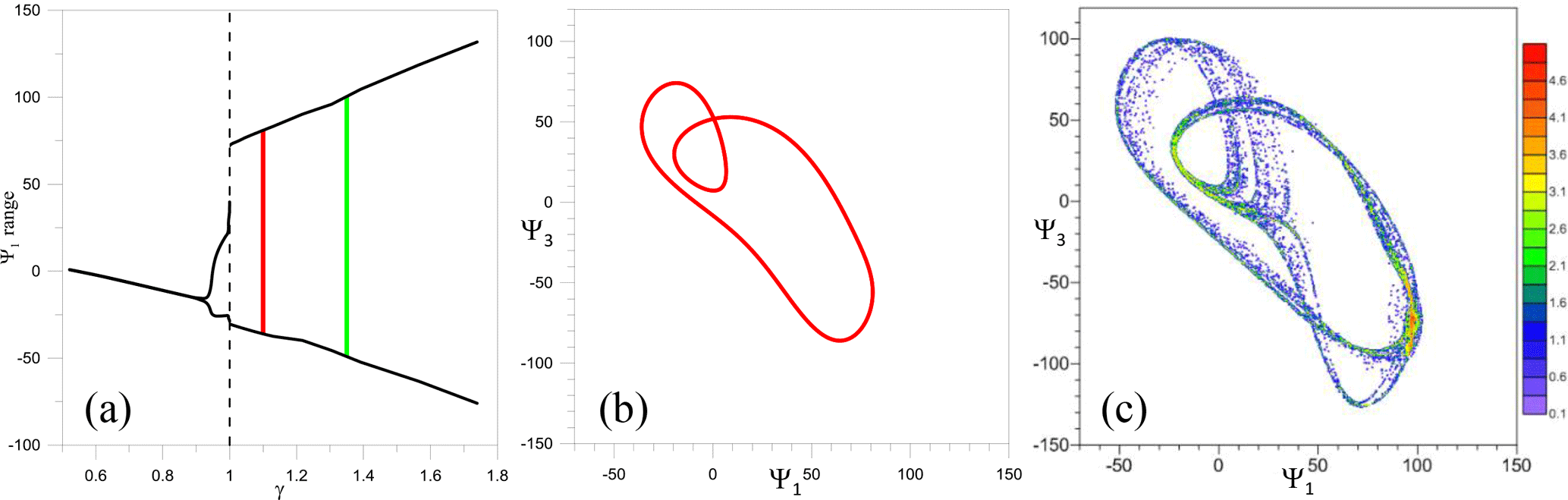
Figure 1 Behavior of the autonomous ocean model, for which ε=0 in Eq. (3). (a) Bifurcation diagram, in which the range of the variable Ψ₁ is plotted vs. the wind stress intensity γ; the two cases γ=1.1 and 1.35 discussed in the text are indicated with a red and a green vertical line, respectively. (b) Limit cycle in the (Ψ₁,Ψ₃) plane, plotted after spinup, that arises from Γ for γ=1.1. (c) Map of the suitably scaled PDF of trajectories given by q_k; see text for details.

The ensembles will consist of 15 000 initial data at t=0 that are regularly spaced either in Ω or in a small subset thereof. For the sake of graphical representation, maps of various quantities will be plotted in the rectangle $\mathrm{\Gamma }\equiv \mathit{\{}-\mathrm{70}\le {\mathrm{\Psi }}_{\mathrm{1}}\le \mathrm{150},-\mathrm{150}\le {\mathrm{\Psi }}_{\mathrm{3}}\le \mathrm{120}\mathit{\}}\subset \mathrm{\Omega }$ that lies in the (Ψ₁,Ψ₃) plane. In the discussion of the results, we will refer, for the sake of simplicity and concision, to the model's trajectories as being defined in the (Ψ₁,Ψ₃) plane but, naturally, the actual trajectories evolve in the full four-dimensional phase space.

3 The autonomous system

3.1 The autonomous model's attractors

We begin by analyzing some basic properties of the autonomous system that will be useful in the subsequent investigation. The bifurcation diagram of Fig. 1a shows the range of variability of Ψ₁ vs. the forcing parameter γ. The value γ=1 corresponds to a global bifurcation that manifests itself by a sudden transition from a small-amplitude limit cycle to a relaxation oscillation with a much higher amplitude. The previous results in this respect (Pierini, 2011; Pierini et al., 2016) will be further bolstered by those in Sect. 5 herein (Figs. 14 and 15), which are based on the diagnostic tool proposed in Sect. 4.2.

Figure 2 Distinct autonomous regime behavior for (a, c) γ=1.1 and (b, d) for γ=1.35. (a, b) Time evolution of $P_{{\mathrm{\Psi }}_{\mathrm{3}}}$ for (a) γ=1.1 and (b) γ=1.35. (c, d) Maps of the mean normalized distance σ for (c) γ=1.1 and (d) for γ=1.35; the points $P_{\mathrm{1}}=(\mathrm{85},\mathrm{100})$ and $P_{\mathrm{2}}=(\mathrm{25},\mathrm{5})$ appear in the panels (c) and (d), respectively. Note the different scales in the two maps; 15 000 trajectories, with regularly spaced initial points in Γ, were used for both maps.

Figure 1b shows the limit cycle in Γ arising from arbitrary initial data for γ=1.1, which corresponds to the red vertical line in the bifurcation diagram of panel (a). For γ=1.35 the attractor is chaotic (green line in panel a; see Sect. 5.1 further below). In this case, the map of the suitably normalized decimal logarithm of the probability density function (PDF) of the trajectories in Γ is plotted in Fig. 1c; it is defined by $q_k\left(t\right)={\log }_{\mathrm{10}}\left[\mathrm{1000}\times n_k\left(t\right)\right]$. Here n_k is the number of trajectories contained at time t in the kth cell belonging to the same regular grid of N square cells of width ΔΨ that is used in our ensemble simulations, with N=15 000 and ΔΨ=2, and it is plotted at $t=T_{\ast }=\mathrm{400}$ years, i.e., after spinup.

In an autonomous dynamical system, the attractors do, by definition, not depend on time, i.e., an attractor is a geometric object in phase space that is fixed in time. However, any attractor that is not a fixed point – whether a limit cycle, torus or strange attractor – can contain time-dependent trajectories. Such ensembles of trajectories arising from specific sets of initial states will be plotted to illustrate the attractors of the autonomous system studied herein.

Following Pierini et al. (2016), in Fig. 2a, b the attractors that correspond to the two cases in Fig. 1b, c are represented by the time evolution of $P_{{\mathrm{\Psi }}_{\mathrm{3}}}\left(t\right)={\log }_{\mathrm{10}}(\mathrm{1000}\times p_{{\mathrm{\Psi }}_{\mathrm{3}}})$, where $p_{{\mathrm{\Psi }}_{\mathrm{3}}}\left(t\right)$ is the PDF of localization of the Ψ₃ variable; see Pierini et al. (2016) for technical details. The dense distribution of $P_{{\mathrm{\Psi }}_{\mathrm{3}}}\left(t\right)$ for γ=1.35, as seen in Fig. 2b, is clearly associated with the chaotic character of the flow, while the periodic distribution of $P_{{\mathrm{\Psi }}_{\mathrm{3}}}\left(t\right)$ that corresponds to γ=1.1 in Fig. 2a is due to the different phases that each trajectory attains on the limit cycle, depending on the initial point.

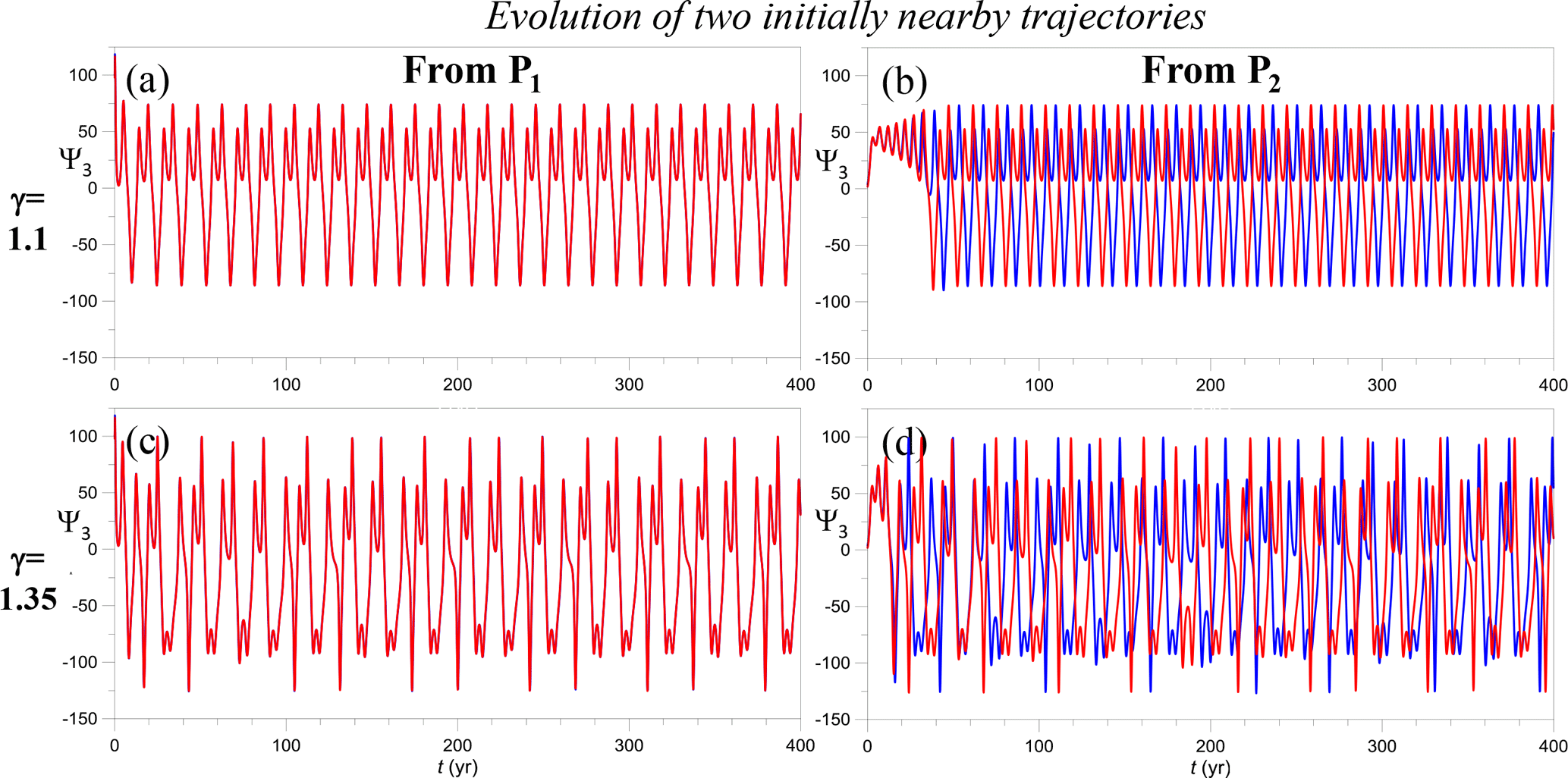
Figure 3 Typical behavior of time evolution of Ψ₃(t) for different values of the parameter γ and different initial points in Γ. (a) Two trajectories obtained for γ=1.1 and initialized at P₁ (red line) and at a nearby point (blue line). (b) Same as in panel (a), but for two trajectories starting from the point P₂ (red) and near it (blue). (c, d) Same as in panels (a) and (b) but for γ=1.35.

In Fig. 2c, d, the same attractors are characterized through the metric σ that was introduced by Pierini et al. (2016); this metric measures the mean divergence of trajectories over the total integration time T_∗ and is defined as follows. The instantaneous Euclidean distance between two initially close trajectories is δ(t), and its normalized value is given by ${\mathit{\delta }}_{\mathrm{n}}\left(t\right)=\mathit{\delta }\left(t\right)/\mathit{\delta }\left(\mathrm{0}\right)$. Then σ is simply the average of δ_n over T_∗,

$$\begin{array}{ll}{\displaystyle }& {\displaystyle }\mathit{\sigma }(X,Y)={\displaystyle \frac{\mathrm{1}}{T_{\ast }}}\underset{\mathrm{0}}{\overset{T_{\ast }}{\int }}{\mathit{\delta }}_{\mathrm{n}}\left(t\right)\mathrm{d}t,\\ \text{(5)}& {\displaystyle }& {\displaystyle }\text{with}(X,Y)\equiv \left({\mathrm{\Psi }}_{\mathrm{1}}\right(\mathrm{0}),{\mathrm{\Psi }}_{\mathrm{3}}(\mathrm{0}\left)\right)\in \mathrm{\Gamma }.\end{array}$$

Pierini et al. (2016) found the quantity σ to be a good indicator of the degree of sensitivity of the system's evolution with respect to the initial state during the phase of convergence to the attractor.

The determination of the PBAs of the periodically forced system and the application of the new qualitative and quantitative diagnostic methods proposed in Sect. 4 need an analysis of the behavior of trajectories that lie at t=0 on a given subset Ω of phase space, as is the case when calculating σ(X,Y) above. Thus, investigating the behavior of model trajectories as they emerge from Ω is the most unifying and distinctive feature of the present model study.

The map of σ in Fig. 2c reveals, in the autonomous case at hand, the same striking features found by Pierini et al. (2016) for the nonautonomous, aperiodic-forcing case, namely the coexistence of extended regions of Γ with σ⩽1, shown by cold colors, and with σ>1, appearing as warm colors. In the first case, two trajectories that are initially close remain close at all times, as seen in Fig. 3a. In the second case, though, two trajectories that are initially close may attain a large phase difference once they have converged to the attractor (cf. Fig. 3b), while still remaining perfectly coherent.

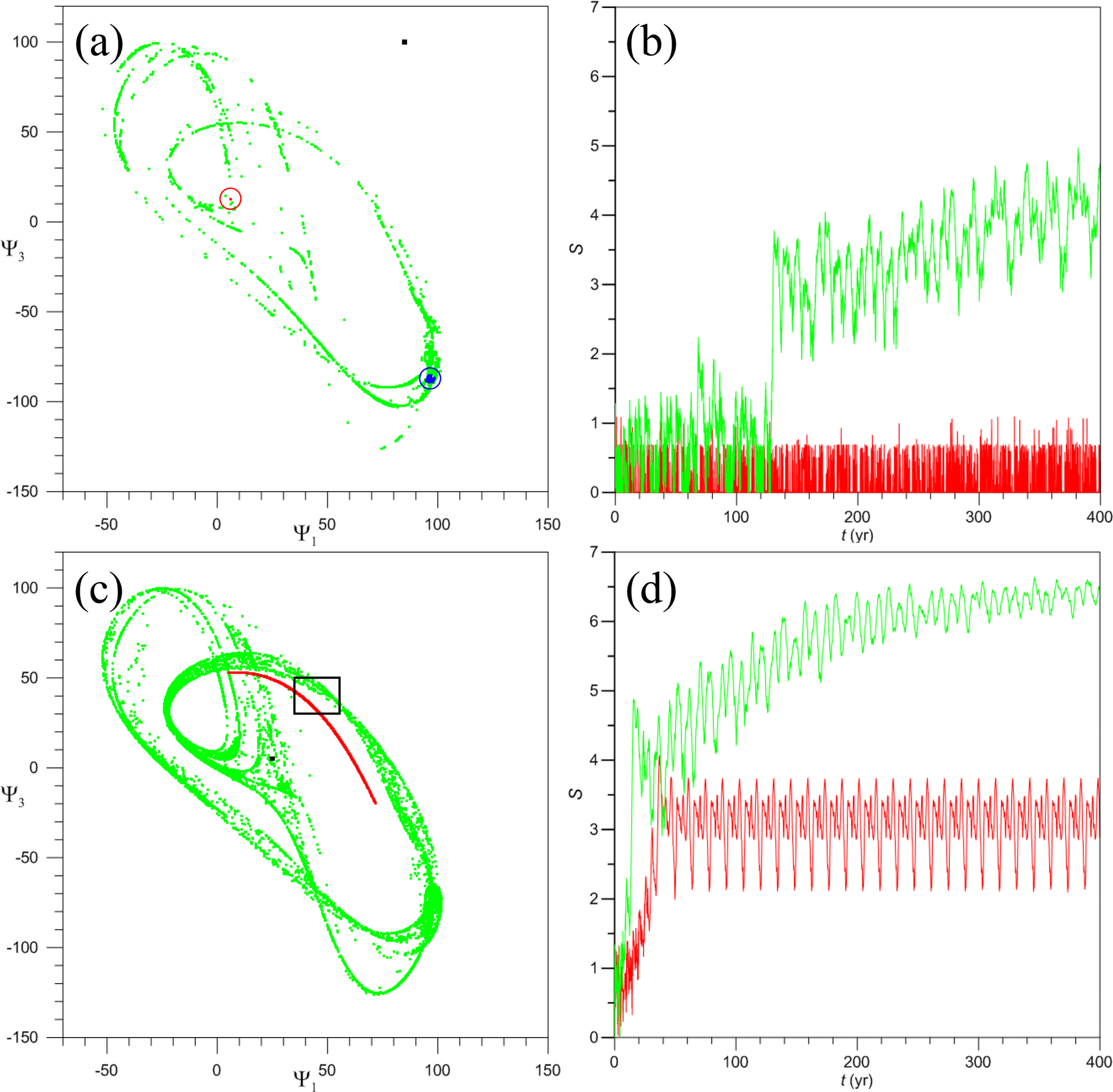
Figure 4 Chaotic and nonchaotic behavior of the autonomous model, for time-independent forcing intensity γ=1.1 (red) and γ=1.35 (green), respectively. Typical behavior of (a, c) the trajectories in the model's phase plane (Ψ₁,Ψ₃) and (b, d) of the model's entropy S_ϑ(t). (a) Intersection with the (Ψ₁,Ψ₃) plane at t=300 years of 15 000 trajectories emanating from the small square box ϑ₁ of width ΔΨ=2 and centered at the point P₁ (black dot), for γ=1.1 (red dots, enclosed in the red circle) and for γ=1.35 (green dots); for the blue dots see the text. (b) Time evolution of the corresponding entropy $S_{{\mathit{\vartheta }}_{\mathrm{1}}}$ for γ=1.1 (red line) and γ=1.35 (green line). (c, d) Same as panels (a) and (b), but for the initial box ϑ₂ centered at P₂, likewise shown as a black dot in panel (c). For the evolution of the points contained at t=300 years in the black rectangle of panel (c), see Fig. 5 below.

In the chaotic case with γ=1.35, the warm-color regions, in which σ>1, overwhelm the cold-color regions, in which $\mathit{\sigma }\le \mathrm{1},$ cf. Fig. 2d. To illustrate the two types of behavior, Fig. 3c, d show the evolution of Ψ₃(t) of two initially nearby trajectories. If σ<1, as is the case near P₁, the two trajectories are virtually coincident (Fig. 3c). If, on the contrary, σ>1, as is the case near P₂, the two aperiodic signals lose their coherence (Fig. 3d). Finally, it is worth noting that, for simulations with sufficiently small γ (not shown), σ<1 everywhere.

A different and useful way of looking at these two types of behavior is to analyze the corresponding mixing properties of the flow in the model's phase space. To do so, one can make use of the system's entropy (Shannon, 1948):

$$\begin{array}{}\text{(6)}& S_{\mathit{\vartheta }}\left(t\right)=-\sum _{k=\mathrm{1}}^N{p}_k\ln p_k.\end{array}$$

Here Γ is decomposed into a regular grid of N square cells of width ΔΨ (with N=15 000 and ΔΨ=2, so that the grid corresponds to that of the initial data used in our ensemble simulations) and p_k(t) is the probability of localization in the kth cell at time t of the trajectories emanating at time t=0 from a given subset ϑ⊂Γ.

Figure 4a shows the intersection with the (Ψ₁,Ψ₃) plane at t=300 years of 15 000 trajectories originating from the box ϑ₁ that coincides with the ΔΨ×ΔΨ grid cell centered at P₁; the red dots correspond to the case γ=1.1 and the green dots to γ=1.35. Figure 4b shows $S_{{\mathit{\vartheta }}_{\mathrm{1}}}$ for the two cases; note that $S_{{\mathit{\vartheta }}_{\mathrm{1}}}\left(\mathrm{0}\right)=\mathrm{0}$ since all the initial states lie in the single cell ϑ₁, and thus p₁=1. The entropy of the periodic case γ=1.1, characterized by σ<1, oscillates between 0 and 1, with the final evolution limited to virtually a single cell over the limit cycle; the latter cell is enclosed in the red circle of Fig. 4a.

In the chaotic case γ=1.35, σ≤1 for 43 % of the points contained in ϑ₁, while σ>1 for the remaining points. The evolution of the former leads to the localized blue dots in Fig. 4a while the evolution of the latter leads to the green dots scattered over the strange attractor. The green line of Fig. 4b, giving $S_{{\mathit{\vartheta }}_{\mathrm{1}}}$ computed with all the trajectories, shows the gradual spreading of the initial points with σ>1.

Figure 4c, d show the same quantities for the initial ΔΨ×ΔΨ box ϑ₂ centered at P₂. The chaotic case is similar to that for ϑ₁, but with a greater entropy; however, the periodic case differs in that now σ>1 – cf. Fig. 2c. Figure 4c shows that the asymptotic evolution of the very small ϑ₂ covers a limited but significant part of the limit cycle, as seen by comparing this figure with Fig. 1b; the corresponding entropy in Fig. 4d eventually oscillates periodically between the values $S_{{\mathit{\vartheta }}_{\mathrm{2}}}\sim \mathrm{2.2}$–3.7. Figure 4 thus demonstrates clearly the usefulness of the metric σ in characterizing subsets of Γ and the effect of the control parameter γ.

Finally, it is worth stressing that, since the forcing is constant, the range of variability of the entropy in the chaotic case with σ>1 must tend to zero as the number of points tends to infinity. This tendency is clearly illustrated by the green line of Fig. 4d. However, the range of variability of $S_{{\mathit{\vartheta }}_{\mathrm{1}}}$ in the chaotic case (Fig. 4b) is still quite large after 400 years because, as pointed out above, the number of points with σ>1 contained in ϑ₁ is relatively small.

3.2 An apparent paradox

We conclude the analysis of the autonomous system by discussing an apparent paradox. We have just seen that, in regions of Γ where σ>1, the trajectories for γ=1.1 exhibit sensitive phase dependence on initial data, as shown, for instance, by Fig. 3b, by the red dots in Fig. 4c and by the red curve in Fig. 4d. Sensitive dependence on initial data is usually associated with chaotic dynamics, but in this case the dynamics are periodic.

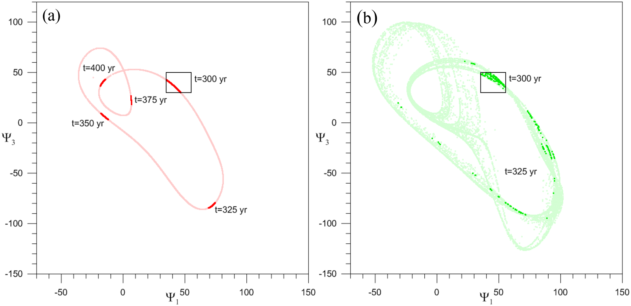
Figure 5 Chaotic and nonchaotic behavior of the autonomous model. (a) Evolution of the 1774 points (red dots) contained at t=300 years in the black rectangle of Fig. 4c for γ=1.1; the attractor is illustrated by the entire set of 15 000 points, shown in light red. (b) Same but for the 135 points (green dots) that lie within the same rectangle for γ=1.35; in this case, the attractor composed of the 15 000 points is shown in light green. Due to the chaotic nature of the dynamics in this case, only one snapshot, after 25 years, is drawn.

This paradox is resolved by noting that such sensitivity concerns only the phase of the periodic trajectories, as already noticed in the previous subsection and, in addition, it occurs only if the initial data lie outside the attractor, e.g, elsewhere on Γ; on the attractor, this phase sensitivity disappears, as we will show below. On the contrary, in the chaotic case γ=1.35, the sensitivity to initial data for trajectories with σ>1 always holds, off the attractor as well as on it. This is in excellent agreement with the chaotic character of the dynamics in the latter case.

We must show, therefore, that the trajectories are stable for γ=1.1 and unstable for γ=1.35, once they have settled onto the attractor. This distinction between the two cases can already be inferred from Figs. 3 and 4 but it is worth investigating the issue in greater detail. The usual quantitative approach relies on the computation of the leading finite-time Lyapunov exponent λ of each trajectory (e.g., Ott, 2002).

The results (not shown) are consistent with the assumption above, but the exponents are highly dependent on the time T_λ over which the finite-time exponents are computed, and on the amplitude of the perturbation superimposed on the reference trajectory at each time step T_λ. Moreover, the assumption of exponential divergence of chaotic trajectories is not fully met in our highly nonlinear framework, so that the transition between periodic and chaotic dynamics may actually occur at a value of λ that is not exactly equal to 0. A qualitative diagnostic method is instead illustrated in Fig. 5, and furthermore we propose an alternative quantitative method in Sect. 4.

Let us consider the points lying in the black rectangle shown in Fig. 4c at t=300 years: the corresponding evolution at four subsequent time instants, T_Δ=25 years, is shown in Fig. 5a for γ=1.1 (red dots). Note that the period of the orbits on the attractor is $T_{\ast }p=\mathrm{14.08}$ years, i.e., $T_{\mathrm{\Delta }}>T_{\ast }p$.

The stability of the trajectories under consideration is clearly demonstrated in Fig. 5a by the compact form and limited extent of the cluster: indeed, these points that start from t=300 years evolve anticlockwise around the attractor, covering it roughly 6 times during the interval 4T_Δ=100 years that separates the first snapshot from the last one. On the contrary, Fig. 5b shows that for γ=1.35 (green dots) the compact form of the initial cluster is lost already after a single 25-year lapse of time. The trajectories will thus soon be scattered over the strange attractor, due to their divergence.

In conclusion, our autonomous system becomes chaotic for sufficiently large values of γ, e.g., for γ=1.35. The system's periodic regime spans a range of γ that includes the bifurcation at γ=1, which is apparent in Fig. 1a.

Moreover, we have shown that, when γ=1.1, regions of Γ exist within which the mean normalized distance σ between two initially nearby trajectories is larger than unity; see again Fig. 2c. In this case, despite the attractor's being a limit cycle, the trajectories leaving from such regions of phase space experience sensitive phase dependence on the initial data. Although sensitive dependence is typically associated with chaotic systems, this sensitivity is not in contradiction with the periodic character of the solutions: as a matter of fact, the trajectories under discussion are stable and the sensitive dependence disappears once the trajectories have converged onto the attractor.

The existence of regions with σ>1 for an autonomous periodic system is an important feature for the transition to chaos when the system is subjected to time-dependent forcing: this issue will be discussed in the next section. Besides, the new diagnostic method introduced in Sect. 4.2 to help analyze transition to chaos in the nonautonomous case will be applied in Sect. 5.1 to the autonomous case.

4 The periodically forced system

For the idealized double-gyre model governed by Eq. (2), we have seen that the autonomous system given by ε=0 in Eq. (3) exhibits a limit cycle when γ=1.1; this limit cycle corresponds to the large-amplitude relaxation oscillation of Fig. 1b. However, Pierini (2014) showed that, when the same model, with the same value of γ, is subjected to periodic forcing with ε=0.2 and T_p=30 years, it exhibits chaotic, cyclostationary and cycloergodic behavior; see Figs. 2 and 3 therein and the related discussion. To understand the transition to deterministically chaotic behavior induced by the forcing, we will now apply in Sect 4.1 the methodology used in Sect. 3 to the attractors corresponding to γ=1.1 and T_p=30 years across the intervening parameter range $\mathrm{0}\le \mathit{\epsilon }\le \mathrm{0.2}$. In Sect. 4.2, the transition to chaos induced by the periodic forcing will be analyzed in greater detail through an additional method here developed explicitly for this purpose.

We know from the rigorous proof of Pierini et al. (2016, Appendix A) that our idealized ocean model possesses a global PBA, in the general case of time-dependent forcing, whether periodic or aperiodic. PBAs are, in fact, time-dependent mathematical objects that characterize the asymptotic behavior of a nonautonomous dissipative dynamical system (e.g., Chekroun et al., 2018, Fig. 2).

Figure 6 Transition from a periodic to a chaotic PBA as the amplitude ε of the periodic forcing in Eq. (3) increases. (a–d) Time evolution of P_Ψ3 and (e–h) maps of σ in the (Ψ₁,Ψ₃) plane for γ=1.1, T_p=30 years and $\mathit{\epsilon }=\mathrm{0},\mathrm{0.05},\mathrm{0.1}$ and 0.2, respectively. Panels (d) and (h) correspond to the reference case studied by Pierini (2014).

It is common, though, in the literature of periodically forced dynamical systems to study the asymptotic behavior of such a system by an iterated stroboscopic map $\mathit{\left\{}u\right(t)\to u(t+T\left)\mathit{\right\}}$, where u is the variable and T is the period. In the particular case in which the system's driver is periodic, so is the PBA; see Sect. 2.3.2 of Chekroun et al. (2018) for a rigorous proof. In contradistinction, a “normal” – i.e., forward rather than pullback – attractor visualized in the embedded space $\left(u\right(t),u(t+T\left)\right)$ and built by using points along a long trajectory $\mathit{\left\{}u\right(t):t_{\mathrm{0}}\le t\le t_{\mathrm{0}}+\mathcal{T}\mathit{\}}$ is static and therefore contains less information than the corresponding PBA, no matter how long the interval 𝒯 may be. Furthermore, PBAs built from ensembles of initial data allow us to visualize in one single picture the coexistence of different types of dynamical behavior in terms of disjoint PBAs; see, for instance, Fig. A2 in Appendix A herein. Besides, the PBA framework is useful for the visualization of fractal structures that arise when noise is superimposed to the periodic forcing. A stroboscopic map analysis may not easily reveal such fractal features; see Chekroun et al. (2011), as well as Sect. 3.4 of Chekroun et al. (2018).

4.1 The pullback attractors of the forced system

For all the above reasons, we now present the PBAs of our periodically forced ocean model. As already just mentioned, the PBAs of a periodically forced dissipative system are always periodic, but the system can be either chaotic or nonchaotic, depending on its parameter values. For the sake of simplicity, we will refer below to the PBAs of a chaotic and nonchaotic system, abbreviated as CPBAs and NPBAs, respectively.

For the autonomous case, the time evolution of P_Ψ3(t) and the map of σ(X,Y) – already shown in Fig. 2a and c, respectively – are again plotted in Fig. 6a and e for the sake of comparison. Figure 6d, h correspond to the reference CPBA studied by Pierini (2014). Note also that one of the two reference cases studied by Pierini et al. (2016) has the same values of γ and ε, but the latter parameter was multiplied by the aperiodic forcing shown in Fig. 17 below. Two intermediate cases that correspond to ϵ=0.05 and ϵ=0.1 are shown in Fig. 6b, f and c, g, respectively. In Sect. 4.2, we will show in greater detail that the transition to chaotic behavior occurs abruptly, when crossing a critical value ϵ_c that lies between the two intermediate values of 0.05 and 0.1; here we merely provide some qualitative arguments showing that, in fact, the case ϵ=0.05 is still periodic, while the case ϵ=0.1 is chaotic.

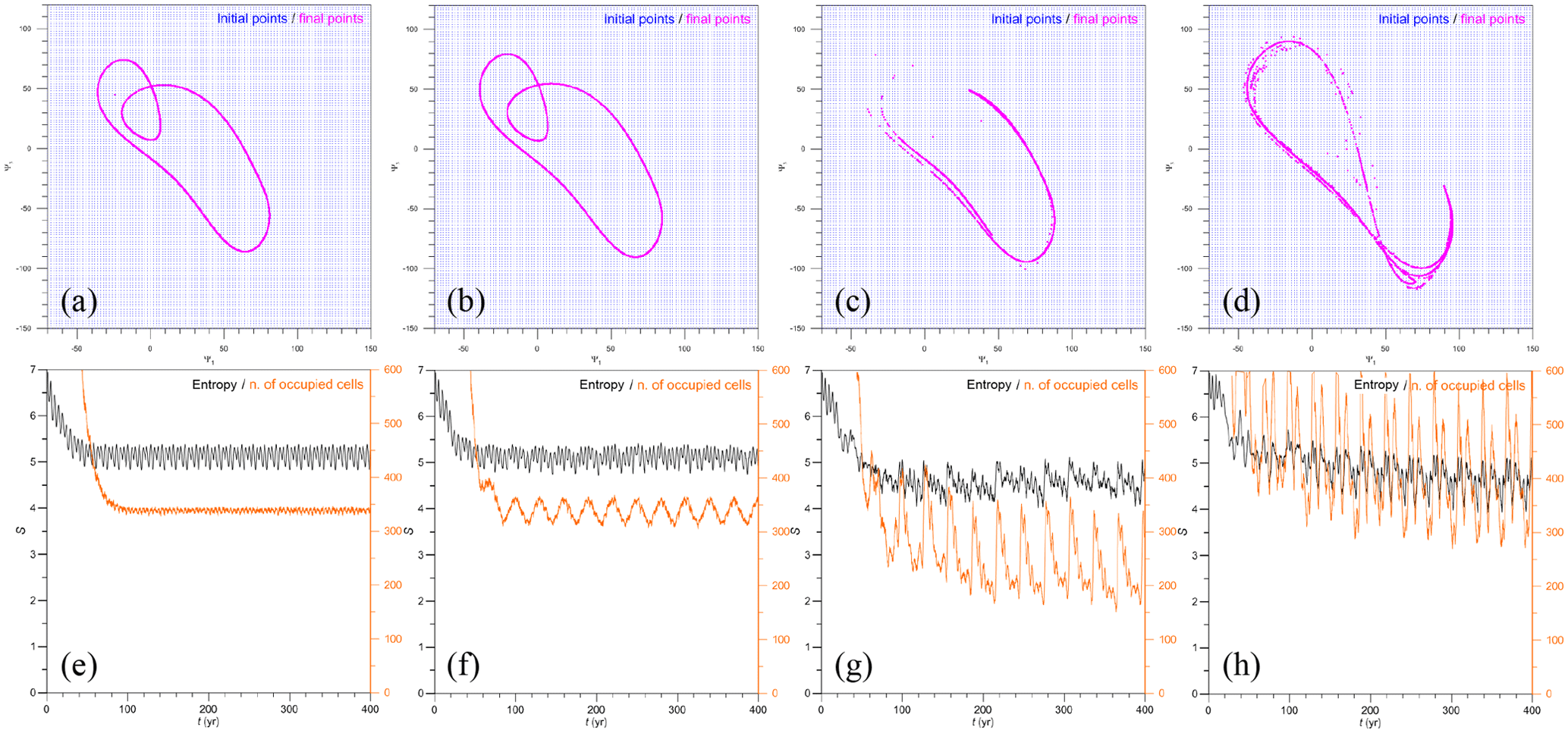
Figure 7 Intersection with the (Ψ₁,Ψ₃) plane at t=400 years (magenta dots) of 15 000 trajectories emanating from Γ at t=0 for γ=1.1 and T_p=30 years. The complete set of the initial points covering Γ is in blue. (a) ϵ=0, (b) 0.05, (c) 0.10, and (d) 0.2. (e–g) The corresponding entropy $S_{{\mathit{\vartheta }}_{\mathrm{2}}}$ is plotted, along with the number n_o of occupied cells.

Before proceeding with the analysis of the results in Fig. 6, we recall that chaotic systems subjected to periodic forcing can be studied either by ensembles of trajectories – as done herein – or by stroboscopic averages using a single long trajectory, provided the assumption of cycloergodicity holds (e.g., Boyles and Gardner, 1983): the latter result extends the classical ergodicity property valid for strange attractors of autonomous systems (e.g., Eckmann and Ruelle, 1985) to chaotic, periodically forced systems. An example of this equivalence is shown in Fig. 3c, d of Pierini (2014) for the present model and for the parameter values corresponding to the P_Ψ3(t) and σ(X,Y) plotted in Fig. 6d, h herein (obviously, the trajectory used in that example was derived from a region with σ>1). However, the existence of regions with σ⩽1, as well as with σ>1, in the two chaotic cases (Fig. 6g, h) shows that the cycloergodicity assumption fails to hold for our idealized ocean model. Our system must, therefore, be investigated using the ensemble approach, which we pursue throughout this paper. In fact, had we only used the stroboscopic map method, we would never have discovered the existence of two types of local attractors, namely CPBAs and NPBAs, in our model.

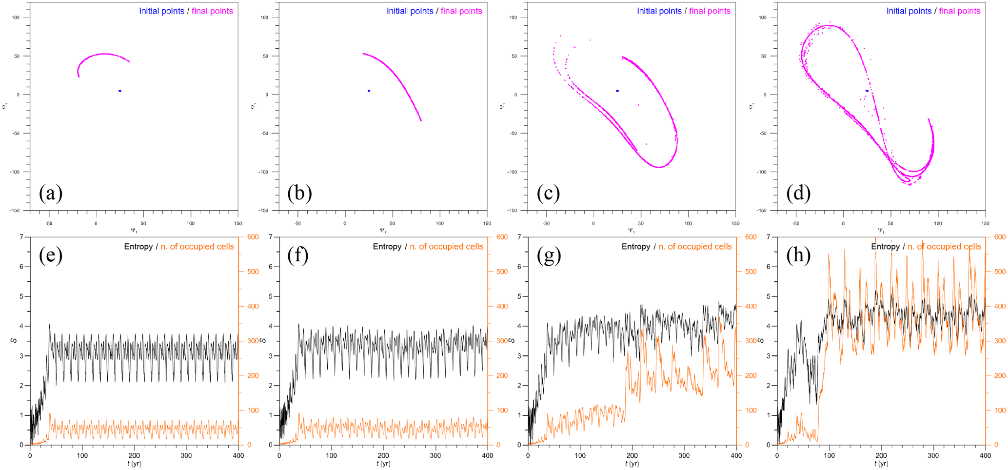
Figure 8 Same as Fig. 7, but for 15 000 trajectories emanating at t=0 from the small rectangle ϑ₂ of width ΔΨ=2 centered at P₂.

Figure 7 provides further information on the four cases illustrated in Fig. 6. In Fig. 7a–d, the magenta dots represent the intersection with the (Ψ₁,Ψ₃) plane at t=400 years of 15 000 trajectories, whose initial points (in blue) are evenly distributed in Γ at t=0; in addition, in Fig. 7e–h, the corresponding entropy S_ϑ=Γ is plotted as a function of time, along with the number n_o of cells that are occupied by at least one point. Clearly, the structure of the PBA snapshot in Fig. 7b, for ε=0.05, is very similar to that of the autonomous case in Figs. 1b and 7a, while the PBA snapshots plotted at t=400 years – for ε=0.1 and 0.2 in Fig. 7c and d, respectively – are quite different.

To understand this difference better, we focused in Fig. 8 on the subdomain ϑ₂ of Γ that was defined in Fig. 4c and for which σ>1. The autonomous case has already been analyzed in Sect. 3.1: in fact, Fig. 8a, e are equivalent to Fig. 4c, d. In the case of ε=0.05, the same behavior is found, i.e., the sensitivity to initial data leads to only a compact subset of the attractor being covered; this implies the periodicity of the trajectories.

On the contrary, for ε=0.1 the intersection of the trajectories at t=400 years with the (Ψ₁,Ψ₃) plane, shown by the magenta dots in Fig. 8c, is virtually indistinguishable from the one that appears in Fig. 7c, when the initial data are selected in the whole of Γ: this excellent match is an unequivocal sign of the mixing property of chaotic dynamics, as already discussed for the autonomous case γ=1.35 in connection with Figs. 4 and 5. That the same property holds for ε=0.2 in Fig. 8d is not surprising, since Pierini (2014) already recognized the model's chaotic behavior for this parameter value.

Figure 9 Increasing instability of trajectories as ε increases. Time evolution of Ψ₃(t) for the trajectory initialized at the point P₂ (red line) and at a nearby point (blue line) for γ=1.1, T_p=30 years, and (a–d) $\mathit{\epsilon }=\mathrm{0},\mathrm{0.05},\mathrm{0.1}$ and 0.2.

Finally, it is instructive to visualize Ψ₃(t) for a couple of trajectories that are very close at t=0, as done in Fig. 3 for the autonomous case. Figure 9 shows Ψ₃(t) for the four cases of Figs. 6–8 and for trajectories that emerge from ϑ₂. In Fig. 9a, b the two trajectories are periodic, but with a phase difference. In the two chaotic cases of ε=0.1, 0.2 in Fig. 9c, d, both trajectories are clearly aperiodic. In Fig. 9c, though, i.e., in the case that is closer to the transition, this aperiodicity is merely associated with a temporary shift in phase of an otherwise periodic signal within the intervals t≃40–120 years and t≃360–400 years.

The intermittent behavior seen in Fig. 9c appears – from many simulations that are not shown here – to be typical of chaotic solutions near the transition point ε_c and suggests a possible mechanism through which chaos is induced by an external periodic forcing. For values of ε just past ε_c, the model still tends to behave periodically, but the external forcing is sufficiently strong to entrain a trajectory occasionally into a nearby region, where the periodicity is preserved but the phase differs by a finite amount. Since these shifts are very sensitive to the initial data, the result is a chaotic trajectory characterized by separate intervals of periodic oscillations with a different phase. This mechanism also explains why the transition to chaos leads to a notable increase in the measure of the regions in Γ where sensitive dependence to initial data occurs; such an increase is visually obvious when comparing Fig. 6e, f with Fig. 6g, h. As ϵ increases further, the duration of the intervals of constant phase decreases, and the oscillations tend to become more genuinely aperiodic, as seen in Fig. 9d.

This behavior is similar to the intermittency found in autonomous dissipative systems (e.g., Manneville and Pomeau, 1979; Pomeau and Manneville, 1980), in which a trajectory switches back and forth from periodic to aperiodic oscillations provided a certain control parameter of the system – e.g., the amplitude of the steady, time-independent forcing – crosses a given threshold. In our nonautonomous system, the amplitude of the periodic forcing ε plays a similar role. This transition to chaos induced by time-dependent forcing appears, therefore, to be directly linked to the existence of regions in phase space in which sensitive dependence to initial data occurs in the limit of periodic solutions. Thus, the chaotic behavior merely due to the time-dependent nature of the forcing can be traced back to the apparently paradoxical property of the autonomous system that was emphasized in Sect. 3.2. This striking observation deserves to be analyzed in greater depth in future studies.

4.2 Transition to chaos studied by a cross-correlation method

Recognizing qualitatively whether a PBA is chaotic or not is relatively simple; e.g., this can be done through the heuristic arguments illustrated in Figs. 4 and 5 and through those outlined in the previous subsection and illustrated in Figs. 6–9. But how does one characterize the transition from periodic to chaotic dynamics as a control parameter, such as the amplitude ε of the periodic forcing, changes?

We have already discussed in Sect. 3.1 the limitations of using the mean finite-time Lyapunov exponents. Here we propose a new, simple and robust method that is particularly useful in our periodic-forcing case, but can be applied also to any autonomous system and even to aperiodically forced systems; the latter situations will be addressed in Sect. 5. In Sects. 3 and 4.1, we have relied on the mixing properties of chaotic dynamics, as measured by the system's entropy S_ϑ, to recognize the occurrence of chaotic behavior. Now we rely on the emergence of aperiodic signals from a subset of Γ; this subset will necessarily be contained in the region where sensitive dependence on initial data occurs, i.e., where σ>1.

The most obvious approach would be to compute the power spectrum of each trajectory. Periodic signals can, however, be quite complex, as seen, for instance, in Fig. 9a, b; this complexity makes it quite difficult to identify a parameter whose value will distinguish, accurately and reliably, between periodic and chaotic dynamics, based solely on the Fourier spectra of a finite number of finite-length trajectories.

We propose a simpler alternative method that takes advantage of the ensemble simulations carried out to obtain the PBAs numerically. Let ${\stackrel{\mathrm{‾}}{\mathrm{\Psi }}}_{\mathrm{3}}$ and ζ₃ be the mean and root-mean square values of ${\mathrm{\Psi }}_{\mathrm{3}}(X,Y,t)$, and consider the centered and normalized anomaly time series ${\stackrel{\mathrm{̃}}{\mathrm{\Psi }}}_{\mathrm{3}}(X,Y,t)$ and ${\stackrel{\mathrm{̃}}{\mathrm{\Psi }}}_{\mathrm{3}}\left(X^{\prime },Y^{\prime },t\right)$, of Ψ₃, with

$$\begin{array}{}\text{(7)}& {\stackrel{\mathrm{̃}}{\mathrm{\Psi }}}_{\mathrm{3}}={\displaystyle \frac{{\mathrm{\Psi }}_{\mathrm{3}}-{\stackrel{\mathrm{‾}}{\mathrm{\Psi }}}_{\mathrm{3}}}{{\mathit{\zeta }}_{\mathrm{3}}}},\end{array}$$

where (X,Y) and $\left(X^{\prime },Y^{\prime }\right)$ are two points in Γ that are near to each other, and from which these two time series emerge at t=0. We can then compute the cross-correlation between the two signals, after removing the initial transient, as

$$\begin{array}{ll}{\displaystyle }& {\displaystyle }c(X,Y,\mathit{\tau })=\\ \text{(8)}& {\displaystyle }& {\displaystyle }{\displaystyle \frac{\mathrm{1}}{T_{\ast }-\mathrm{2}T}}\underset{T}{\overset{T_{\ast }-T}{\int }}{\stackrel{\mathrm{̃}}{\mathrm{\Psi }}}_{\mathrm{3}}\left(X,Y,t\right){\stackrel{\mathrm{̃}}{\mathrm{\Psi }}}_{\mathrm{3}}(X^{\prime },Y^{\prime },t+\mathit{\tau })\mathrm{d}t;\end{array}$$

here $T_{\ast }=\mathrm{400}$ years is again the maximum integration time, and $-T\le \mathit{\tau }\le T$, while T=50 years; once more, the following results are independent of T, provided it is sufficiently larger than the typical timescale of the phenomenon. Note also that, in the above definition, we have dropped the dependence of c on $(X^{\prime },Y^{\prime })$ for the sake of conciseness.

Now, if σ<1, the two signals are periodic and virtually coincident, as seen, for instance, in Fig. 3a, c. Hence, defining the maximal cross-correlation by

$$\begin{array}{}\text{(9)}& \mathrm{\Theta }(X,Y)=max\left\{c\left(X,Y,\mathit{\tau }\right):\mathit{\tau }\in \left[-T,T\right]\right\},\end{array}$$

one will have $\mathrm{\Theta }(X,Y)\cong \mathrm{1}$, with Θ being attained at τ=0.

However, if σ>1, there are two possibilities:

• either the PBA is not chaotic, in which case all couples (X,Y) and $(X^{\prime },Y^{\prime })$ yield two periodic and virtually equal signals, apart from a finite phase difference, as seen, for instance, in Figs. 3b and 9a, b; in this case, again, Θ≅1, which will now occur at some lag τ≠0 that depends on the phase difference;

• or the PBA is chaotic, in which case all couples yield two aperiodic and significantly different signals, as seen, for instance, in Figs. 3d and 9c, d; in this case, Θ will be substantially less than unity.

This alternative is illustrated in Fig. 10 for the four couples of trajectories plotted in Fig. 9a–d, all of which were initialized in ϑ₂, where σ>1.

It is then useful to analyze the maps of the parameter Θ. Figure 11a–d show Θ for the four cases of Figs. 6–9. In the two cases that we have already identified as nonchaotic, Θ varies within a range of values [0.95,1.1] that lies very close to unity, as expected; see Fig. 11a, b. There is only a small neighborhood of $P_{\mathrm{0}}=(-\mathrm{16},-\mathrm{83})$ in which Θ is very small: this is because P₀ in the autonomous case is a fixed point; see Fig. 12.

The two cases that we have identified as chaotic appear here as Fig. 11c, d, and in them Θ exhibits in fact smaller values. These values lie in the range [0.2,0.8] for a large subset of the domain, where σ>1, as shown in Fig. 6g, h. Regions in which σ>1 but Θ≃1 are present as well, but the corresponding trajectories are nonetheless unstable once they have converged onto the PBA, because they will always pass sufficiently near trajectories that are chaotic, thanks to the mixing properties of the latter.

In summary, if Θ∼1 everywhere (yellow colors) we have an NPBA, whereas if Θ yields values that are sufficiently smaller than unity (grey colors) then we have a CPBA.

To summarize in a clear and simple way the information provided by the values of both σ and Θ, we introduce the integer-valued parameter Φ, defined as follows:

$$\begin{array}{}\text{(10)}& \mathrm{\Phi }\left(X,Y\right)=\left\{\begin{array}{l}\mathrm{1}\text{ if }\mathit{\sigma }\mathit{⩽}\mathrm{1}\left(\mathrm{yellow}\right),\\ \mathrm{2}\text{ if }\mathit{\sigma }>\mathrm{1}\mathrm{and}\mathrm{\Theta }>{\mathrm{\Theta }}_{\mathrm{0}}\left(\mathrm{green}\right),\\ \mathrm{3}\text{ if }\mathit{\sigma }>\mathrm{1}\mathrm{and}\mathrm{\Theta }\mathit{⩽}{\mathrm{\Theta }}_{\mathrm{0}}\left(\mathrm{red}\right).\end{array}\right.\end{array}$$

Here Θ₀ is a threshold value and Φ(X,Y) is plotted in Fig. 11e–h for Θ₀=0.8.

As an example of the usefulness of Φ, let us note that the σ maps in Fig. 6f and g are fairly similar, except for the more extended warm-color region, where σ>1, in the second map. Recall, however, that the meaning of σ>1 is profoundly different if the system is chaotic, in which case mixing is present, as opposed to when it is not, in which case sensitive dependence to initial data concerns only the phase of the signal and is not accompanied by mixing. This ambiguity is resolved by the use of the step function Φ: if ϵ=0.05 (Fig. 11f), sensitive dependence to initial data, i.e., σ>1, yields the value of Φ=2 (green regions), since Θ≃1, which tells us that the system is not chaotic. On the contrary, if ϵ=0.1 (Fig. 11g), regions with Φ=2 (in red) appear within the green regions: this implies low Θ values and therefore chaos.

Figure 10 Cross-correlation c(τ) between the two initially nearby trajectories shown in Fig. 9a–d, computed for the centered and normalized anomalies ${\stackrel{\mathrm{̃}}{\mathrm{\Psi }}}_{\mathrm{3}}$, according to Eq. (6), for ε=0 (red line), 0.05 (orange line), 0.1 (green line) and 0.2 (blue line).

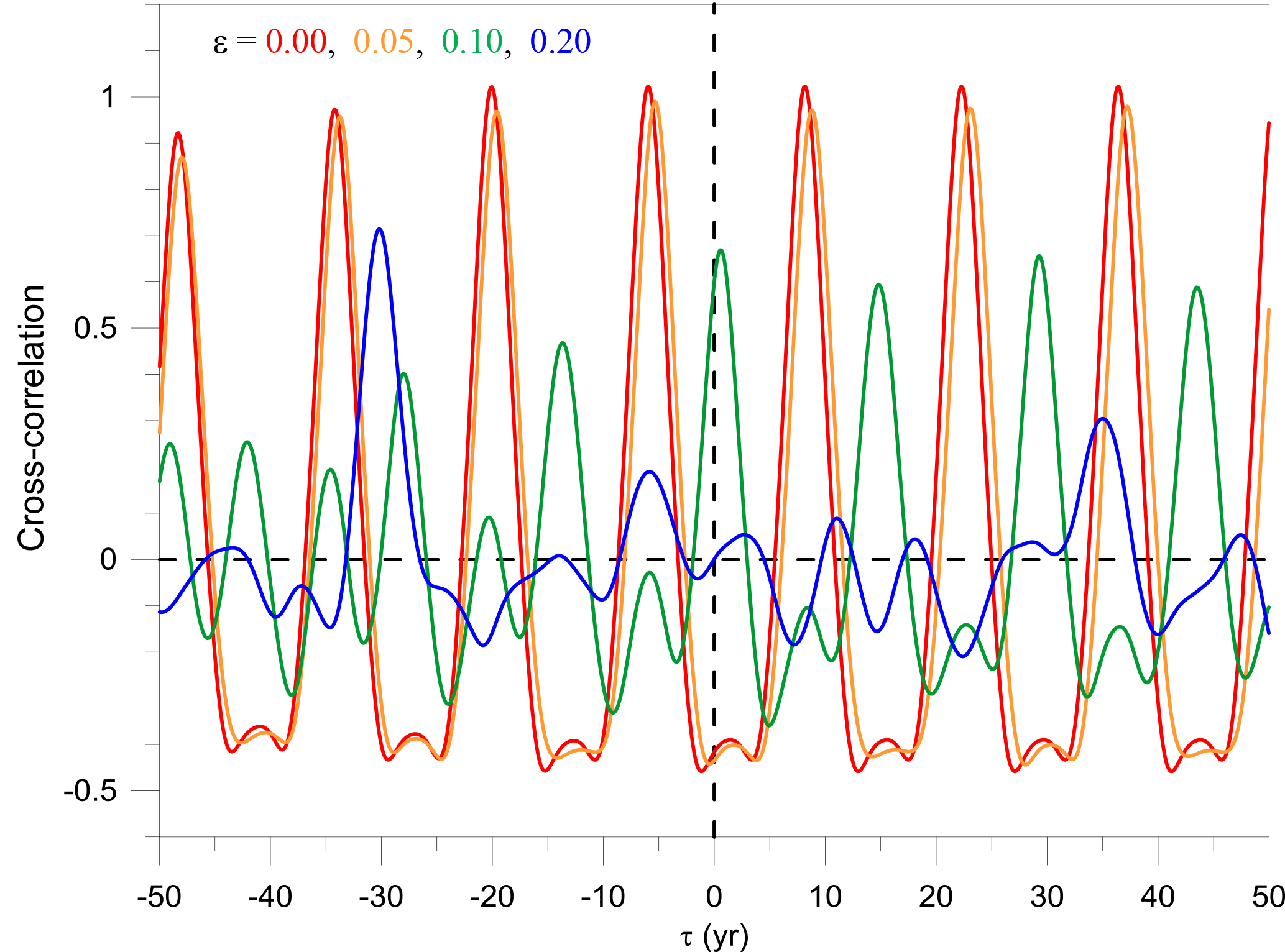
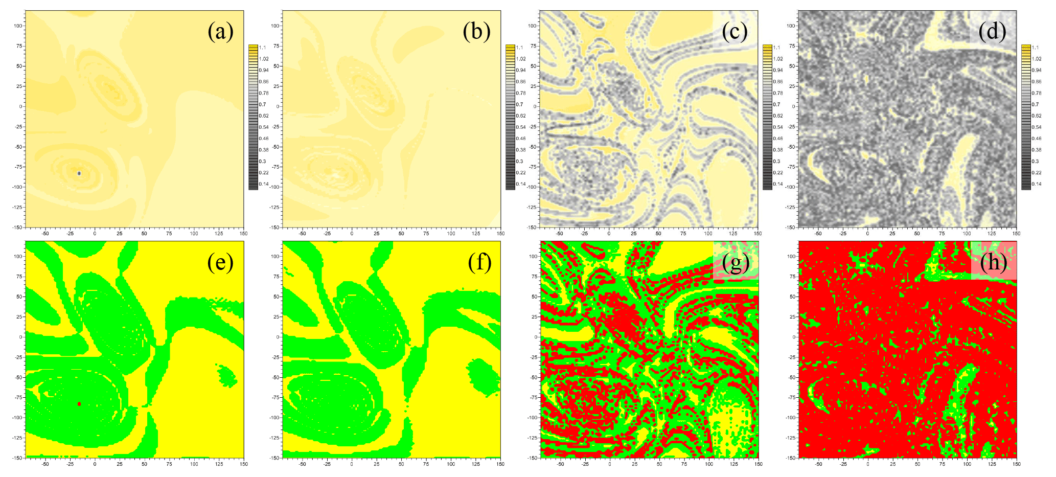
Figure 11 PBA diagnostics for γ=1.1 and T_p=30 years, with $\mathit{\epsilon }=\mathrm{0},\mathrm{0.05},\mathrm{0.1}$ and 0.2, respectively, for the two sets of four maps. Upper-row panels (a)–(d) show the field of Θ(X,Y) in the (Ψ₁,Ψ₃) plane, as defined in Eq. (7); the color bar for the Θ(X,Y) values is shown to the right of each panel, and it extends over the range [0.1,1.12]. Lower-row panels (e)–(h) show the field of Φ(X,Y) in the (Ψ₁,Ψ₃) plane, as defined in Eq. 8, with the threshold value Θ₀=0.8; here Φ=1 is colored yellow, Φ=2 is green and Φ=3 is red. The corresponding maps of σ(X,Y) appear in Fig. 6e–h, respectively.

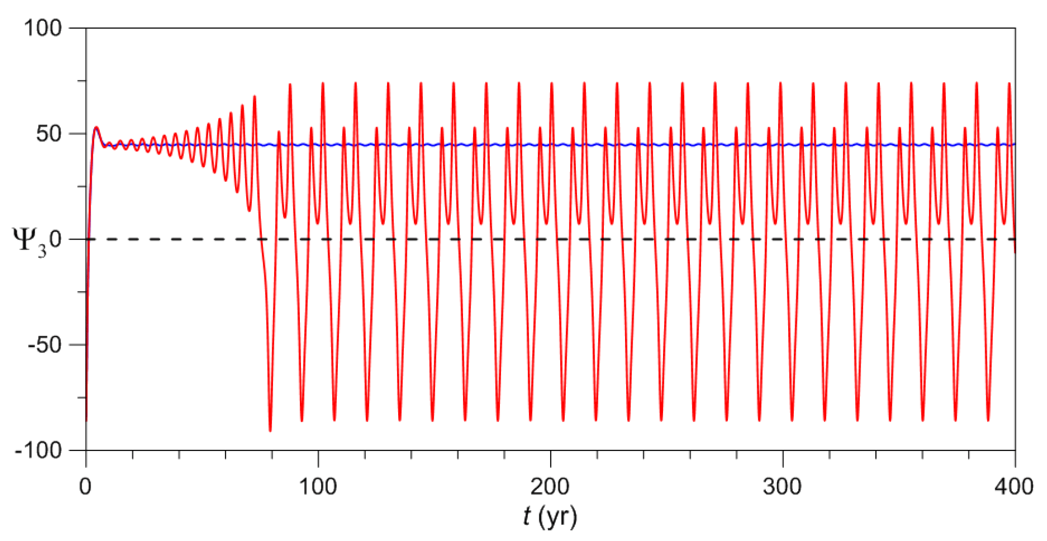
Figure 12 Fixed point P₀ of the autonomous case, with ε=0. Time evolution of Ψ₃ for the trajectory initialized at $P_{\mathrm{0}}=(-\mathrm{16},-\mathrm{83})$ (blue line) and at a nearby point (solid red line) for γ=1.1 and T_p=30 years.

We conclude by analyzing the transition from NPBAs to CPBAs via a suitable function of the control parameter ε: this metric is provided by the average value 〈Θ〉_Γ of Θ over Γ. The graph of 〈Θ〉_Γ(ε) in Fig. 13 is obtained by performing many ensemble simulations of system trajectories with many distinct values of ε; the latter values are chosen to lie closer to each other, where the variation in 〈Θ〉_Γ(ε) is stronger. An abrupt transition from NPBAs, with 〈Θ〉_Γ≃1, to CPBAs occurs at ε_c≅0.09. Many additional analyses (not shown) for values just below and above ε_c confirm that this is in fact the critical value beyond which chaos sets in.

5 Further applications of cross-correlation diagnostics

5.1 Application to the autonomous system

The diagnostic method proposed in Sect. 4.2 to monitor the transition from NPBAs to CPBAs in periodically forced systems relies on two properties: (i) in an NPBA all trajectories are periodic, and (ii) in a CPBA diverging aperiodic trajectories emerge from a subset of Γ, in which necessarily σ>1. Thus, the same cross-correlation-based method can obviously be applied to an autonomous system as well. The method's application to the autonomous model studied in Sect. 3 will shed new light on the periodic vs. chaotic character of its solutions.

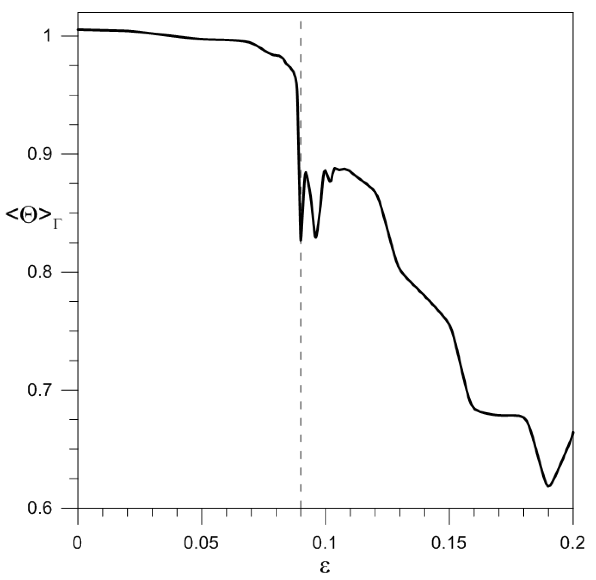
Figure 13 Transition from periodic to chaotic behavior, illustrated by the metric 〈Θ〉_Γ plotted vs. the amplitude ε of the periodic forcing in Eq. (3); γ=1.1 and T_p=30 years.

The graph in Fig. 14 shows 〈Θ〉_Γ(γ) and is obtained, like that of Fig. 13, by performing many ensemble simulations, each with a different value of γ, rather than ε, which equals zero in the present case. The first thing to notice is the sudden drop of 〈Θ〉_Γ at $\mathit{\gamma }={\mathit{\gamma }}_{\mathrm{c}}=\mathrm{1}$, where a global bifurcation separates small-amplitude limit cycles from large-amplitude relaxation oscillations, as shown in Pierini (2011) and in Sect. 3.1 here. In addition, Pierini (2012) investigated the stochastic version of this deterministic tipping point in the case of random forcing.

The chaotic nature of the attractor for γ_c is illustrated in Fig. 15. For γ=0.99, the Ψ₃ time series exhibits the typical small-amplitude, purely periodic behavior studied in Sect. 3.1, while for γ=1 both small- and large-amplitude oscillations occur irregularly in the same time series. The behavior at γ=1.01 illustrates the return to more regular behavior.

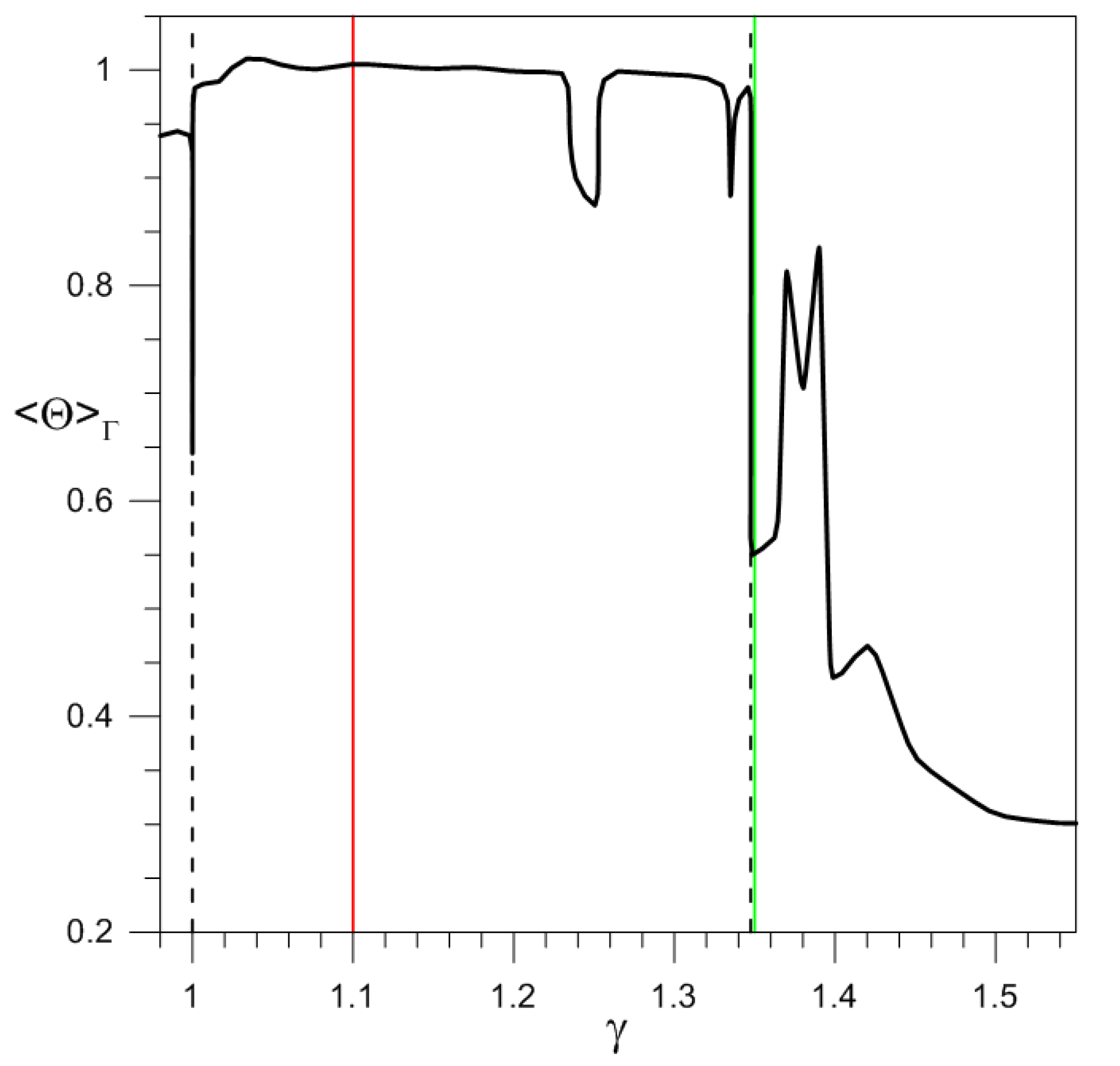
Figure 14 Same as Fig. 13, but for the autonomous model with ε=0 and the amplitude γ of the time-independent forcing on the abscissa. The vertical red and green lines denote the periodic and the chaotic cases, respectively, that were analyzed in Sect. 3.1; see again Fig. 1. Please see the text for the interpretation of the dashed lines corresponding to γ_c=1 and γ₀=1.3475.

Figure 15 Critical transition in the autonomous system at γ_c. Panels (a) and (d), (b) and (e), and (c) and (f) correspond to $\mathit{\gamma }=\mathrm{0.99},\mathrm{1.0}$ and 1.01, respectively. (a–c) Time evolution of Ψ₃ for the trajectory initialized at P₁ (red line) and at a nearby point (blue line); (d–f) same but for trajectories initialized at P₂.

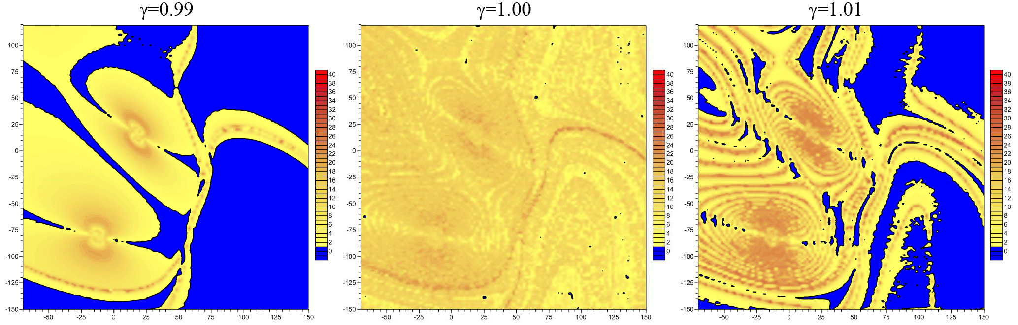
Figure 16 Critical transition in the autonomous system at γ_c, illustrated by maps of the mean normalized distance σ in the (Ψ₁,Ψ₃) plane for γ=0.99, 1.0 and 1.01.

Thus, chaotic dynamics occurring in an extremely restricted γ range separates two different types of limit cycles. Figure 16 shows this dramatic transition in terms of σ: the chaotic nature of the flow for γ_c=1 is such that the warm-colored regions in which σ>1 overwhelm the cold-colored regions, as in Fig. 2d, where $\mathit{\gamma }=\mathrm{1.35}.$

For γ>1, the system is not chaotic – except for limited γ intervals centered at γ≃1.25 and γ≃1.335 – until a new abrupt drop of 〈Θ〉_Γ at $\mathit{\gamma }={\mathit{\gamma }}_{\mathrm{0}}=\mathrm{1.3475}$, shown by a dashed black line in Fig. 14. This drop signals the presence of chaotic attractors beyond γ₀; in particular, the chaotic case γ=1.35, shown by the solid green line and discussed in Sect. 3, lies just after this transition. It is worth noting that large fluctuations dominate the chaotic regime.

5.2 Application to an aperiodically forced system

Our cross-correlation diagnostics have been shown to apply to both periodically forced and autonomous systems. Its validity, however, is even more general, since it extends to a large class of aperiodically forced systems as well. We choose the model setup of Pierini et al. (2016) to illustrate the latter possibility. A thorough analysis of this application is beyond the scope of the present study: we will therefore limit ourselves to analyzing the basic aspects of the problem and leave the details for a future investigation.

Pierini et al. (2016) considered the same system – governed by Eq. (2), and within the same parameter regime adopted here and in Pierini (2011). The forcing, though, was aperiodic and given by the following:

$$\begin{array}{}\text{(11)}& G\left(t\right)=\mathit{\gamma }\left[\mathrm{1}+{\mathit{\epsilon }}^{\prime }f\left(t\right)\right],\end{array}$$

where ${\mathit{\epsilon }}^{\prime }>\mathrm{0}$ is a dimensionless coefficient and f(t) is a normalized, fixed realization of an Ornstein–Uhlenbeck process that has been smoothed to resemble multi-annual wind-stress forcing of the midlatitude oceans' double-gyre circulation. Figure 17 shows G(t) for γ=1 and ${\mathit{\epsilon }}^{\prime }=\mathrm{0.2}$.

Figure 18 shows the evolution of two initially nearby trajectories emerging from P₂, along with the corresponding cross-correlation, for γ=1.1, with ${\mathit{\epsilon }}^{\prime }=\mathrm{0.05}$ in panels (a–b) and ${\mathit{\epsilon }}^{\prime }=\mathrm{0.20}$ in panels (c–d); both cases have σ>1 and the corresponding time series of $P_{{\mathrm{\Psi }}_{\mathrm{3}}}$ are plotted in Fig. 4h, j of Pierini et al. (2016). The case ${\mathit{\epsilon }}^{\prime }=\mathrm{0.2}$ corresponds to the CPBA analyzed in detail by Pierini et al. (2016). The chaotic character of the solution is clearly visible from Fig. 18c; the cross-correlation between the two signals is plotted in Fig. 18d and it is accordingly small.

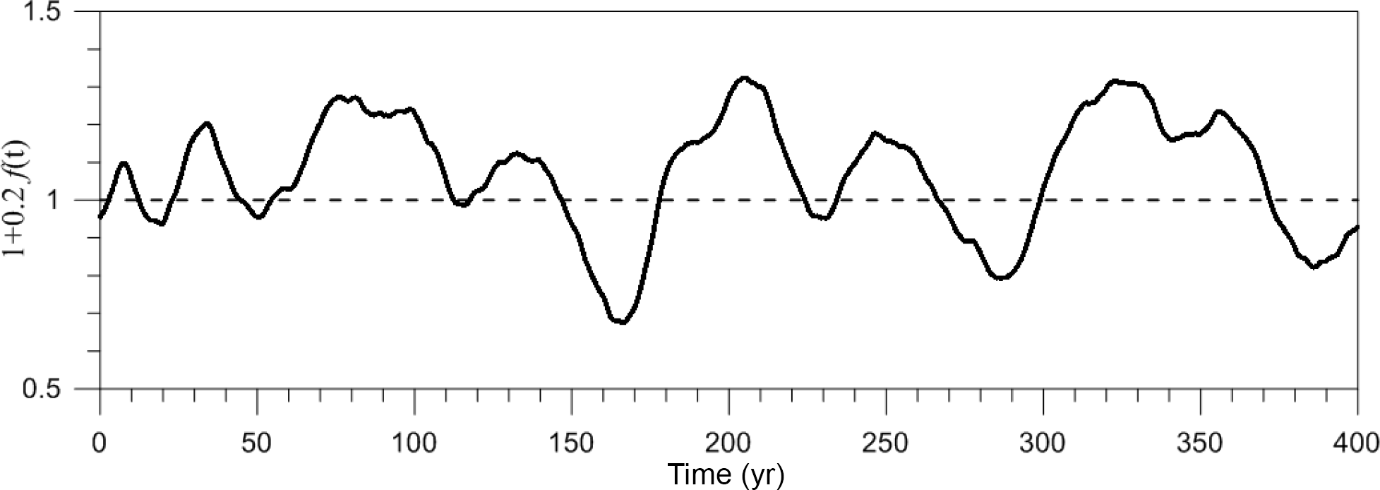
Figure 17 Aperiodic forcing G(t)∕γ of the idealized ocean model – defined by Eq. (9) herein, and plotted using the value ${\mathit{\epsilon }}^{\prime }=\mathrm{0.2}$, as adopted in Pierini et al. (2016).

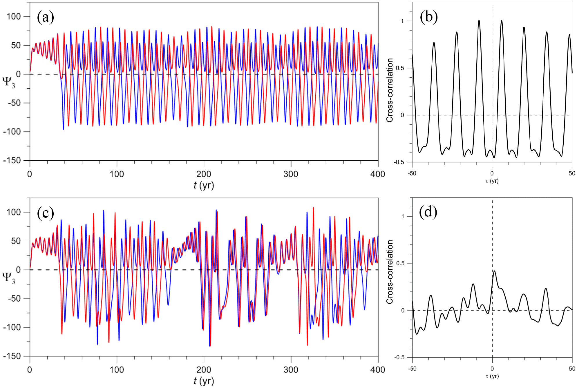
Figure 18 Role of the cross-correlation diagnostics in characterizing chaotic behavior for an aperiodically forced system, given by Eqs. (2) and (9); γ=1.1. (a) Time evolution of Ψ₃ for ${\mathit{\epsilon }}^{\prime }=\mathrm{0.05}$ in Eq. (9) and (b) corresponding cross-correlation. (c, d) Same as panels (a) and (b) but for ${\mathit{\epsilon }}^{\prime }=\mathrm{0.2}$. The trajectories initialized at P₂ are in red and those initialized at a nearby point are in blue.

On the contrary, the case ${\mathit{\epsilon }}^{\prime }=\mathrm{0.05}$ corresponds to an NPBA: the two signals in Fig. 18a develop a large phase difference after the initial transient, but are virtually identical and remain coherent at all times. Now, unlike in Figs. 3b and 9a, b, the two signals are not periodic because they are modulated by the aperiodic forcing, but this is irrelevant; in fact, the nonchaotic character of the solution can still be highlighted by the corresponding cross-correlation in Fig. 18b, whose maximum value is Θ≃1, like in the autonomous and periodically forced case. Obviously, this is possible because the period of the modulated relaxation oscillation is much smaller than the timescale of the forcing; this is in fact the only condition required for the applicability of this diagnostic method to aperiodically forced systems.

We can therefore conclude that the parameter 〈Θ〉_Γ can be a valuable tool for monitoring the onset of chaos in aperiodically forced systems as well. For example, this diagnostic method can be applied to study the onset of chaos in systems that possess a drift mimicking global warming and other climate change scenarios (as done, for instance, in Drótos et al., 2015).

6 Summary and conclusions

In this paper, we studied the transition from nonchaotic to chaotic PBAs in a nonautonomous system whose autonomous limit is nonchaotic, and in which, therefore, chaos is induced by the periodic forcing. The illustrative example chosen for this general problem was a low-order quasigeostrophic model of the midlatitude wind-driven ocean circulation, subject to periodic forcing. The model was described and connected with previous work in Sect. 2.

We first investigated, in Sect. 3, the autonomous system, following up on the work of Pierini (2011), who obtained its governing equations and analyzed their solutions. Here, ensemble simulations based on a large number of initial data and the calculation of the system's entropy allowed us to determine novel and interesting features of the system subject to steady forcing.

To do so, we used the metric σ that was introduced by Pierini et al. (2016) and measures the time average of the distance between two trajectories that are very close at t=0 on a subset Γ of phase space. The analysis based on this metric yielded regions in Γ with σ values that can be either larger or less than unity. The spatial structure of these regions (cf. Fig. 2c, d here) is very similar to that of the nonautonomous case investigated by Pierini et al. (2016), as seen in Fig. 6 therein. This similarity suggests that the nonautonomous behavior of a dynamical system is profoundly influenced by the convergence properties of trajectories initialized off the attractor in the autonomous case; this finding, in turn, implies that ensemble simulations are very helpful in studying said properties.

Next we investigated, still in the autonomous case, the apparent paradox of regions with σ>1 coexisting in the periodic regime of γ=1.1 with the expected regions of σ<1. A large number of trajectories emanating from the small square box of Fig. 4c, for which σ>1, evolves into the extended red line shown in the same figure at a given time, t=300 years: this line belongs to the periodic attractor shown in Fig. 1b and the entropy evolution along it oscillates periodically (cf. Fig. 4d); but it is clearly distinct from the chaotic attractor apparent as the green cloud of points in the same figure panel. Further evidence for the stability of the trajectories in this periodic case with σ>1 is provided by Fig. 5a.

We conclude that sensitive phase dependence on initial data in a periodic regime may be present if the trajectories are initialized off the attractor, but that it disappears once the trajectories have converged onto the attractor. Clearly, generic sensitive dependence on initial data is, therefore, a necessary but not sufficient condition for chaotic behavior.

In Sect. 4, we studied the onset of chaos in the system subject to the periodic forcing given by Eq. (3) in the case of γ=1.1, in which the system is nonchaotic in the autonomous limit, so that chaos is induced by the periodic forcing. The PBAs were analyzed at first for four different sinusoidal-forcing amplitudes, with $\mathit{ϵ}=\mathrm{0},\mathrm{0.05},\mathrm{0.10}$ and 0.2, while using the same γ=1.1 and T_p=30 years.

We found that the first two cases, namely ϵ=0 and 0.05, are nonchaotic, while the other two, namely ϵ=0.10 and 0.20, are chaotic. A large number of trajectories emanating from the small square box where σ>1 in Fig. 8a–d evolves – depending on the value of ε – into two very different fixed-instant subsets of the model's PBA, with the snapshot taken at t=400 years, i.e., after convergence of the trajectories to the PBA. In the first two cases, this snapshot is a curved-line segment that belongs to the PBA, while in the latter two cases it covers the whole PBA, due to the typical mixing property of chaos.

An analysis of the trajectories, as shown in Fig. 9, for instance, indicates that the transition to chaos occurs via an intermittent emergence of periodic oscillations with different phases; see again Fig. 9c. We have shown that, for values of ϵ in the chaotic regime just above the transition, the periodic character of the system is still predominant, but the external forcing is now sufficiently strong to cause a trajectory's occasionally shifting to a phase space region in which a different phase prevails: since the shifts are very sensitive to the initial data, the result is a chaotic trajectory characterized by irregular jumps of the oscillatory solutions between distinct phases.

In Sect. 4.2, we introduced a novel diagnostic method for the study of the transition between nonchaotic and chaotic behavior as the amplitude ϵ of the periodic forcing increases. The method's basic idea is that in a nonchaotic regime any couple of initially nearby trajectories emerging from Γ remain coherent at all times, while in a chaotic regime aperiodic diverging trajectories emerge from a subset of Γ. Hence, a systematic recognition of the character of all the trajectories allows one to diagnose which of these two types of behavior occurs or whether the two actually coexist.

A simple and robust way to do this is to compute the cross-correlation $c(X,Y,X^{\prime },Y^{\prime },\mathit{\tau })$ at lag τ between two initially nearby trajectories started at (X,Y) and $(X^{\prime },Y^{\prime })$ in Γ, then compute its maximum value Θ(X,Y) over τ. If $\mathrm{\Theta }(X,Y)\simeq \mathrm{1}$ everywhere in Γ, then the system is nonchaotic and is therefore periodic under periodic forcing; on the contrary, if Θ is appreciably smaller than unity in some subset of Γ, the system is chaotic. The diagram of the average 〈Θ〉_Γ(ϵ) of Θ(X,Y) over Γ, as plotted in Fig. 13, reveals an abrupt transition to chaos at ϵ_c≃0.09.

This cross-correlation-based method has also been applied to the autonomous system, in which the conditions required for the periodically forced case do apply as well. The diagram of 〈Θ〉_Γ(γ) in Fig. 14 reveals that chaotic dynamics occur at first within an extremely restricted range centered at the global bifurcation point $\mathit{\gamma }={\mathit{\gamma }}_{\mathrm{c}}=\mathrm{1}$, which separates small-amplitude, fairly smooth oscillations below γ_c from large-amplitude relaxation oscillations above it. A considerably broader range of chaotic behavior occurs in the autonomous case for values of γ greater than a threshold γ₀=1.3475.

We have then applied the cross-correlation-based method to the aperiodically forced system studied by Pierini et al. (2016). Our results show that, in fact, this method can be applied to systems subject to aperiodic forcing when the system's intrinsic periodicity and the characteristic timescale of the external forcing are sufficiently well separated from each other, which is the case in Pierini et al. (2016); cf. Fig. 17 here. Once more, the cross-correlations in Fig. 18c, d agree remarkably well with the character of the model trajectories in Fig. 18a, b.

Finally, the coexistence of local PBAs with chaotic vs. nonchaotic behavior within a global PBA – as first described by Pierini et al. (2016) in the aperiodic-forcing case – was confirmed here for the periodically forced case; cf. Figs. 6 and 11. This situation was explored in greater depth in Appendix A for an even simpler, weakly dissipative nonlinear model, namely a Van der Pol–Duffing oscillator (e.g., Jackson, 1991), and additional references were given for this type of PBA bistability.

Overall, this paper provides additional insights into the complex and varied behavior that arises even in highly idealized atmospheric, oceanic and climate models from the interaction of nonlinear intrinsic dynamics with various types of external forcing. In addition, it stresses the importance of using the framework of nonautonomous dynamical systems and of their PBAs for a deeper understanding of this complexity and variety.

Appendix A: Coexistence of pullback attractors in a Van der Pol–Duffing oscillator

The purpose of this Appendix is to provide further insight into the coexistence of local PBAs with quite different stability properties, as illustrated in the main text by Figs. 6 and 11. In complex autonomous systems, several local attractors may coexist for a given set of the system's parameters; each of these attractors possesses attracting sets of initial data that are typically separated by fractal boundaries (Grebogi et al., 1987). Basins of attraction with fractal boundaries have consequences for predictability: uncertainties in the initial state x₀ may result in different types of dynamical behavior, depending on which basin x₀ lies in; see, for instance, Roques and Chekroun (2011). When the number of the coexisting attractors is two, one speaks of bistability, and multistability refers colloquially to more than two coexisting attractors.

Our goal here is to illustrate how multistability of nonautonomous systems manifests itself unambiguously through the existence of disjoint local PBAs. In the case of periodically forced systems, such as those considered in this article, similar results can be inferred, of course, from the analysis of Poincaré maps. Nevertheless, the presence of other frequencies in the internal dynamics, the external forcing or the noise may render the analysis of Poincaré maps difficult, whereas the framework of PBAs naturally includes such additional levels of complexity (Chekroun et al., 2018). Pierini et al. (2016), for instance, already demonstrated the usefulness of this framework in the context of bistability.

Furthermore, the purpose of this Appendix is also to illustrate that multistability of local PBAs arises not only for our quasigeostrophic model, as discussed in the paper's main text. More generally, PBA coexistence occurs fairly often for externally forced systems, although a careful analysis of the flow's dependence on initial data may be required in practice in order to conclude on multistability.

A paradigm of multistability is provided by dissipative nonlinear systems that become Hamiltonian in the limit of vanishing dissipation, as is the case, for instance, in celestial mechanics (e.g., Ghil and Wolansky, 1992). In this situation, it is expected that the number of coexisting attractors exceeds any fixed bound in approaching this limit, as documented for various nearly integrable maps and flows; cf. Feudel et al. (1996), Zaslavsky and Edelman (2008), Celletti (2009), Pisarchik and Feudel (2014) and Dudkowski et al. (2016), and references therein.

To illustrate this multistability phenomenon, we consider the following periodically forced Van der Pol–Duffing oscillator, given by the second-order nonlinear (ordinary differential equation) ODE:

$$\begin{array}{}\text{(A1)}& \ddot{x}=\mathit{\mu }(\mathrm{1}-{\dot{x}}^{\mathrm{2}})x-b{x}^{\mathrm{3}}+F\sin \left(\mathit{\omega }t\right),\end{array}$$

where μ, b, F and ω are positive constants that determine the dynamical behavior of the system. This system is nonautonomous and its PBAs are analyzed hereafter in the $(x,\dot{x})$ plane. This nonlinear ODE arises in various applications such as in engineering, electronics, biology and neurology (Jackson, 1991; Kozlov et al., 1999; Kuznetsov et al., 2009). It combines the nonlinearity of the dissipation $-\mathit{\mu }{\dot{x}}^{\mathrm{2}}x$, which characterizes the Van der Pol (1920) oscillator with that of the internal force −bx³, which characterizes the Duffing (1918) oscillator.

Multistability was already numerically documented for Eq. (A1) by relying on Poincaré maps (Venkatesan and Lakshmanan, 1997; Dudkowski et al., 2016). In our calculations, we have followed Dudkowski et al. (2016) and assumed μ=0.2, $F=b=\mathrm{1.0}$ and ω=0.955. While this parameter regime does not correspond to the limit of vanishing dissipation that was mentioned above, it still allows for a coexistence of PBAs, given a careful choice of initial states.

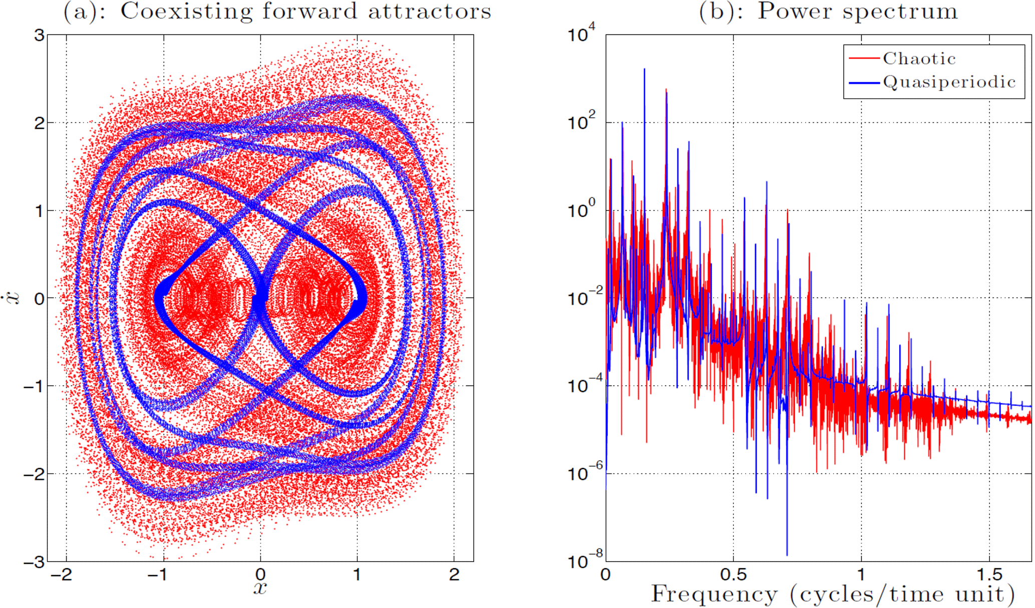
Figure A1 Coexistence of local forward attractors. (a) Quasiperiodic forward attractor (blue) and chaotic attractor (red). (b) Power spectrum associated with the quasiperiodic orbit (blue) and the chaotic one (red).

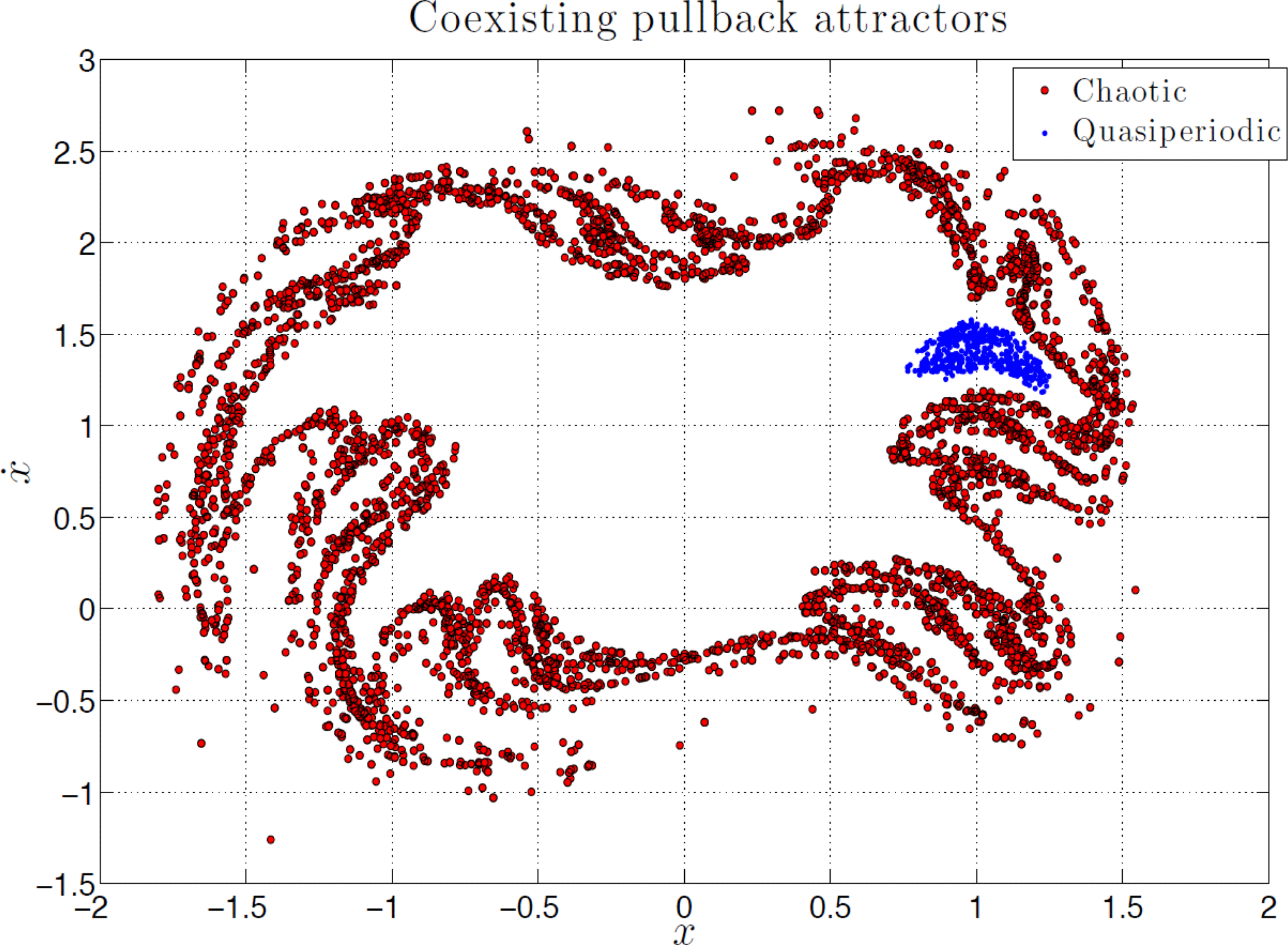
Figure A2 Coexistence of local PBAs. The initial data leading to quasiperiodic (and chaotic) orbits are taken from the small domain D₂ (and D₁) described by Eq. (A2). The snapshot of the PBAs shown here is taken at the fixed time t=2000.

Figure A3 Return maps of the minima of x(t) for (a) the quasiperiodic orbit shown in blue in Fig. A1(a), and for (b) the chaotic orbit shown in red in Fig. A1a; see text for details.

The numerical protocol followed to analyze multistability for Eq. (A1) in terms of PBAs is described next. First, the initial data have been drawn uniformly in the two disjoint domains D₁ and D₂ of the $(x,\dot{x})$ plane, with

$$\begin{array}{ll}{\displaystyle }& {\displaystyle }{D}_{\mathrm{1}}=[-\mathrm{2.5},-\mathrm{1.5}]\times [-\mathrm{2.5},-\mathrm{1.5}],\\ \text{(A2)}& {\displaystyle }& {\displaystyle }{D}_{\mathrm{2}}=[-\mathrm{0.34},-\mathrm{0.33}]\times [-\mathrm{0.34},-\mathrm{0.33}].\end{array}$$

A total of 6000 initial data from each domain were propagated according to Eq. (A1). The ODE was integrated using a Runge–Kutta fourth-order method with a constant time step $\mathrm{\Delta }t={\mathrm{10}}^{-\mathrm{2}}$, generating a total of 12 000 trajectories and keeping 10⁶ data points for each, after removal of the transient.

The majority of the initial data taken in the smaller domain D₂ leads to a quasiperiodic orbit, while each of the 6000 initial data taken in D₁ leads to a chaotic trajectory – as do a few “rare” initial data from D₂. An example of such a quasiperiodic trajectory is shown in blue in Fig. A1a, within the $(x,\dot{x})$ phase plane. This blue trajectory is superimposed upon a red, chaotic trajectory emanating from an initial point taken in D₁. The corresponding power spectra are shown in Fig. A1b, with the same blue and red color coding. The chaotic trajectory is clearly more diffuse within the phase plane than its quasiperiodic counterpart, and its power spectrum is quite a bit noisier. Both of these features are well known to be symptomatic of deterministic chaos (Eckmann and Ruelle, 1985).

By allowing the quasiperiodic trajectories that emanate from D₂ to evolve up to t=2000, one obtains the set of blue points shown in Fig. A2. Somewhat surprisingly, this set does not form a closed curve: each blue dot in Fig. A2 actually corresponds to the state at t=2000 in the phase plane of a quasiperiodic orbit. One such orbit is represented in blue in Fig. A1a, after removal of the transient dynamics. Each blue dot in Fig. A2 corresponds to a different quasiperiodic orbit, whose frequency characteristics may change slightly from one blue dot to another. All these quasiperiodic orbits share, however, a spectral signature that resembles the one shown by the blue curve in Fig. A1b.

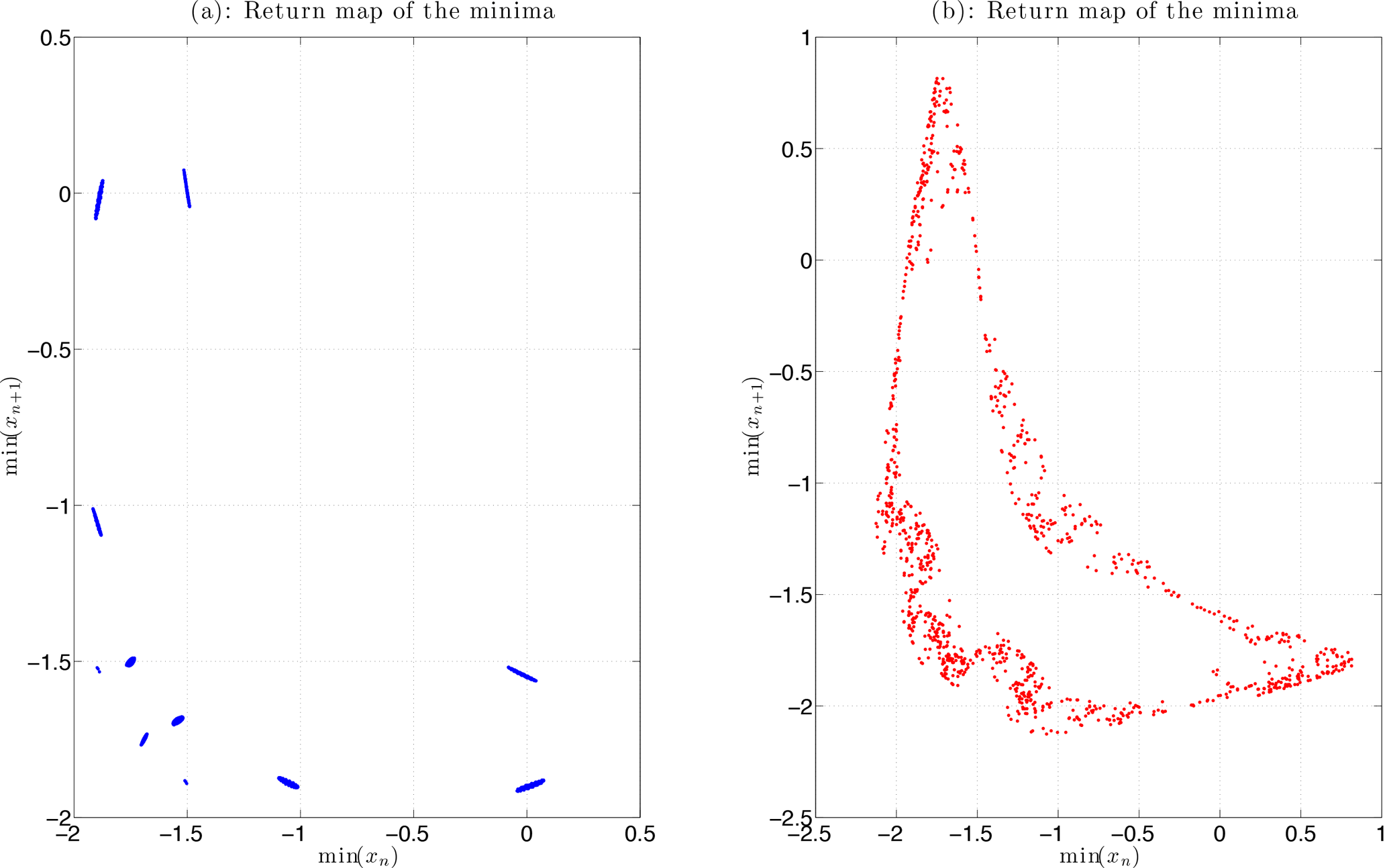
To illustrate further the distinction between quasiperiodic and chaotic orbits, the return maps for the minima of the x(t) variable have been computed. As is well known (e.g., Strogatz, 2015), if the return map contains just one point, the solution is periodic in time, with all minima having the exact same value, and the period of the oscillation can be estimated by calculating the time interval between two consecutive minima. If the return map contains continuous-looking curves that fill up with more and more points as the length of the orbit increases, the solution is quasiperiodic, while the presence of folds and self-similarity in the return map provides strong evidence for chaotic solutions. For the blue and red trajectories of Fig. A1a, we plot the corresponding return maps in Fig. A3a and b, respectively. The two plots clearly discriminate between the quasiperiodic nature of the former and the chaotic nature of the latter solution.

The initial data taken in D₁, when allowed to flow according to Eq. (A1), lead to a totally different local PBA that is formed by the red points shown in Fig. A2. Although the approximation of this local PBA shown here is relatively sparse, one can clearly discern the fact that its constitutive points are arranged according to a stretching and folding pattern that is typical of nonlinear, chaotic dynamics in the autonomous as well as in the nonautonomous setting (Chekroun et al., 2018).

The features that we find here to be exhibited by the local chaotic PBA are highly reminiscent of those that were obtained, in this deterministic case, by applying a standard Poincaré section analysis; cf. Dudkowski et al. (2016, Fig. 17c). In the presence of noise, though, the fine structure of the PBAs that results from stretching and folding in phase space is still captured by the PBA framework (Chekroun et al., 2018), whereas a Poincaré-map approach would lead only to a cloud of points with no particular geometric structure. This statement was numerically illustrated by Chekroun et al. (2011) in their Fig. 7, by contrasting the upper-right panel vs. the six lower panels of that figure.

Finally, we emphasize that it is not the disjointness of the two domains, D₁ and D₂, that leads to the two distinct types of PBA, chaotic and quasiperiodic.¹ Indeed, as mentioned earlier, even though the area of D₂ is small, it still contains initial data whose evolution lands within the local PBA associated with chaos, i.e., with the other red points shown in Fig. A2.