Ensemble variational assimilation as a probabilistic estimator – Part 2: The fully non-linear case

The method of ensemble variational assimilation (EnsVAR), also known as ensemble of data assimilations (EDA), is implemented in fully non-linear conditions on the Lorenz-96 chaotic 40-parameter model. In the case of strong-constraint assimilation, it requires association with the method of quasi-static variational assimilation (QSVA). It then produces ensembles which possess as much reliability and resolution as in the linear case, and its performance is at least as good as that of ensemble Kalman filter (EnKF) and particle filter (PF). On the other hand, ensembles consisting of solutions that correspond to the absolute minimum of the objective function (as identified from the minimizations without QSVA) are significantly biased. In the case of weak-constraint assimilation, EnsVAR is fully successful without need for QSVA.

1 Introduction

In the first part of this work (Jardak and Talagrand, 2018), the technique of ensemble variational assimilation (EnsVAR), which achieves exact Bayesian estimation in the conditions of linearity and Gaussianity, has been implemented on two chaotic toy models with small dimension. The first model was the 40-parameter model introduced by Lorenz (1996). A linearized version was used as reference for the case where exact Bayesianity is achieved. Experiments were then performed with the full non-linear model over assimilation windows for which a linear approximation is almost valid for the temporal evolution of the uncertainty. Although non-linear effects are distinctly present, the statistical quality of the ensembles produced by EnsVAR is as good as in the linear case. The second model was the Kuramoto–Sivashinsky equation (Kuramoto and Tsuzuki, 1975, 1976). Similar conclusions were obtained.

EnsVAR is implemented in this second part, still on the Lorenz (1996) model, over assimilation windows for which a linear approximation is no longer valid. It is implemented first in the strong-constraint case (Sect. 2), where it turns out to be necessary to use it together with the method of quasi-static variational assimilation (QSVA), introduced by Pires et al. (1996). The performance of EnsVAR is compared with that of ensemble Kalman filter (EnKF) and particle filter (PF) in Sect. 3. EnsVAR is then implemented in the weak-constraint case (Sect. 4), where the use of QSVA turns out not to be necessary. Conclusions are drawn in Sect. 5. The general conclusion is that, in the conditions of our experiments, EnsVAR is as successful in non-linear as in linear situations.

Except when explicitly mentioned (and that will be the case mostly concerning the length of the assimilation windows and the number N_win of realizations over which diagnostics are performed), the experimental set-up will be the same as in Part 1. In particular, the size of the ensembles N_ens=30 will always be the same. And, unless specified otherwise, the space–time distribution of observations will also be the same (one complete set of observations of the state variable twice a day, with white-in-space-and-time noise, with standard deviation σ=0.63).

Notations such as Eq. (I-3) or Fig. I-2 will refer to equations or figures of Part 1 (Jardak and Talagrand, 2018).

2 Strong-constraint assimilation

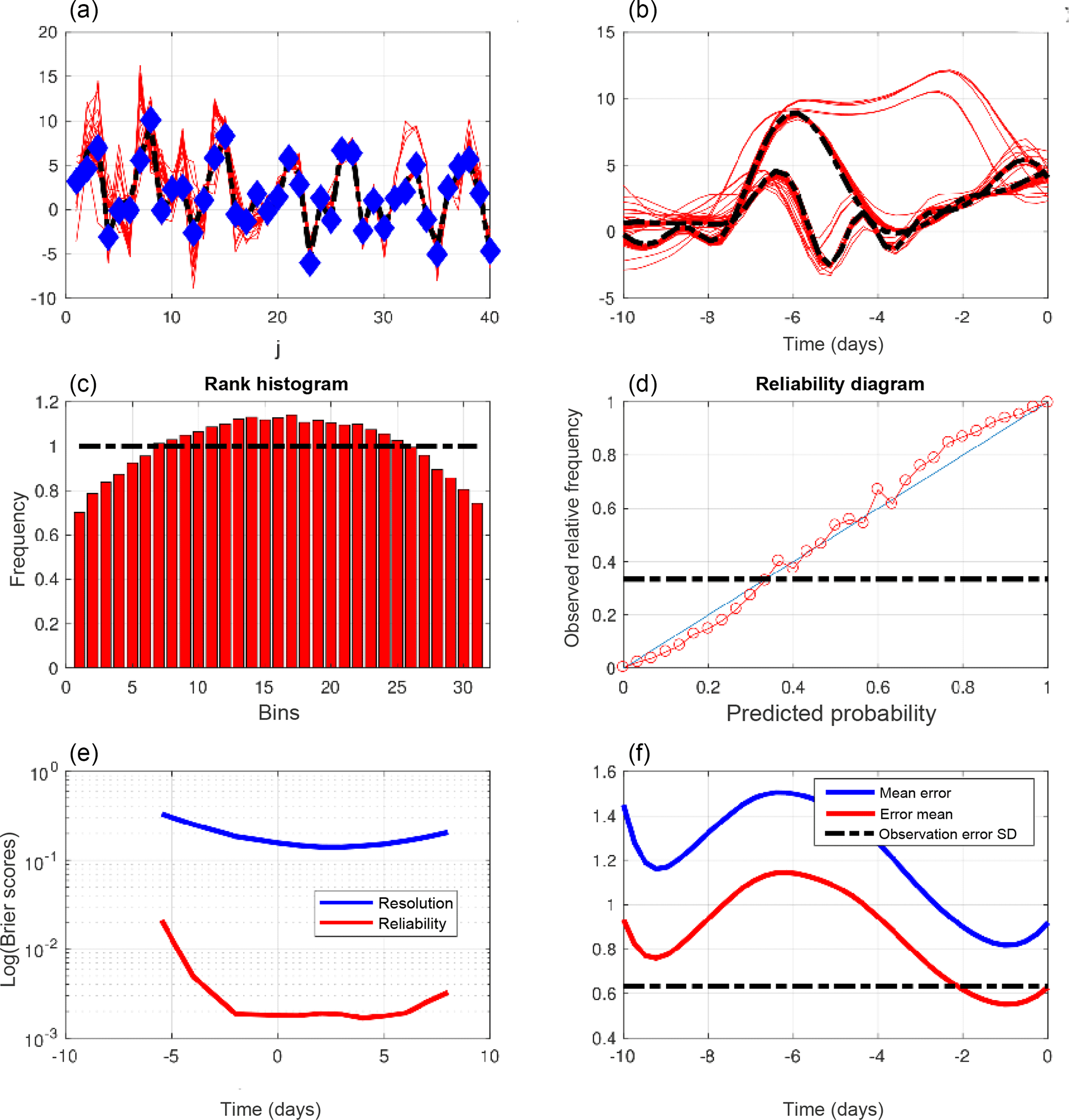
Figure 1 Diagnostics of an experiment performed in the same conditions as for Figs. I-4 and I-5, with the only difference being that the length of the assimilation windows is now 10 days. (a) Truth (dashed black curve), observations (blue dots), and minimizing solutions (red curves) at the initial time of one assimilation window, as functions of the spatial coordinate. (b) Truth (dashed curves) and minimizing solutions (red curves) as functions of time at two grid points over one assimilation window. (c) Rank histogram for the variable x over all grid points and ensemble assimilations. (d) Reliability diagram for the event {x<1.14}, which occurs with frequency 0.35 (dashed–dotted horizontal curve), built over all grid points and ensemble assimilations. (e) Components of the Brier score for the events $\mathcal{E}=\mathit{\{}\mathit{x}<\mathit{\tau }\mathit{\}}$, evaluated over all grid points and ensemble assimilations, as functions of the threshold τ (red curve: reliability, blue curve: resolution). (f) Average RMS errors to truth, as functions of time over assimilation windows. Blue curve: error in individual assimilations. Red curve: error in mean of ensembles (the black dashed–dotted curve shows the standard deviation of observational error).

Figure 1 shows the same diagnostics as Figs. I-4 and I-5, for an experiment in which the length of the assimilation window is 10 days instead of 5. Comparison with Figs. I-4 and I-5 shows an obvious degradation of the quality of the assimilation. The top panels (to be compared with the top panels of Fig. I-4) show that the dispersion of the minimizing solutions is now much larger. That dispersion is statistically much too large can be seen from the rank histogram (middle-left panel), which has a distinct humpback shape, meaning that the verifying truth is much too often located in the central part of the ensembles. The error from the truth is now larger than the observational error (bottom-right panel), which is an obvious proof of failure of the assimilation process. The reliability diagram (middle-right panel) differs slightly, but markedly, from the diagram in Fig. 1.5 through its sigmoid shape. That can easily be verified to be consistent with the overdispersion seen on the rank histogram. And both Brier scores (bottom-left panel) are significantly larger than in Fig. I-5.

Another diagnostic is given in Fig. 2, which shows the histogram of the minimizing values of the objective function (I-9) (the format is the same as in Fig. I-3). The histogram is clearly bimodal. The values in the left mode have expectation 387.1 and standard deviation 18.8, in good agreement with the values of 400 and 20 indicated by the χ² linear theory (Eqs. I-10–I-11; note that because of the increase in the length of the assimilation window from 5 to 10 days, the value of the parameter p∕2 is now 400). This is to be noted since there is a priori no reason to expect that minimizations that lead to the left mode correspond to errors ϵ_k and δ_k (Eqs. I-7–I-8) distributed in such a way as to verify conditions (I-10–I-11). The right mode in Fig. 2 is outside the linear approximation. It is also worth mentioning that out of 270 000 values of 𝒥_min, only 96 330 were situated in the left mode.

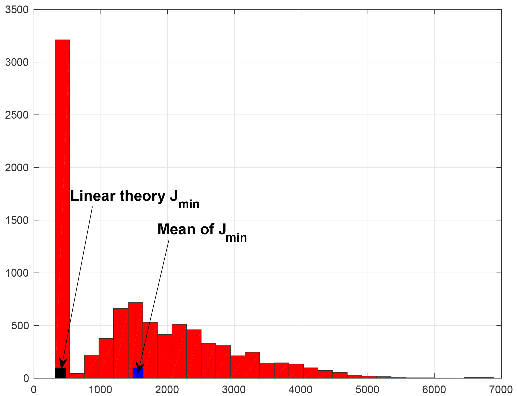
Figure 2 Histogram of (half) the values of the minima of the objective function (I-9), for the same experiment as in Fig. 1.

These results tend to confirm the interpretation that was given of results obtained in Part 1 (see Fig. I-7 and associated comments). This agrees with the discussion and conclusions of the paper by Pires et al. (1996). Because of the chaotic character of the motion, the uncertainty in the position of the observed system is located on a folded subset in state space. The longer the observation period is, the more folded the uncertainty subset is. Secondary minima of the objective function (I-9) may occur on the various folds (for more on this point, see Figs. 4 and 5 of Pires et al., 1996, and the discussion therein). With this interpretation, the left mode on Fig. 2 corresponds to absolute minima and the right mode to secondary ones. Also, because of the longer assimilation window, the basin of attraction of the absolute minimum is narrower than that of Part 1, and more minimizations lead to a secondary minimum. A related discussion can be found in Ye et al. (2015).

Pires et al. (1996) showed that, in the case of noisy observations of chaotic motion, the location of the absolute minimum of the objective function is not significantly affected by the observational noise. It makes therefore sense to locate that absolute minimum. To that end, they proposed the method of quasi-static variational assimilation (QSVA). In that method, the length of the assimilation window is gradually increased, keeping the same initial time, with each new minimization being started from the result of the previous one.

This is what has been done here. Figure 3, which is in the same format as Fig. 1, depicts the results produced by the use of quasi-static variational assimilation over an overall 10-day assimilation window, with an increment of 1 day for the gradual increase in the assimilation window.

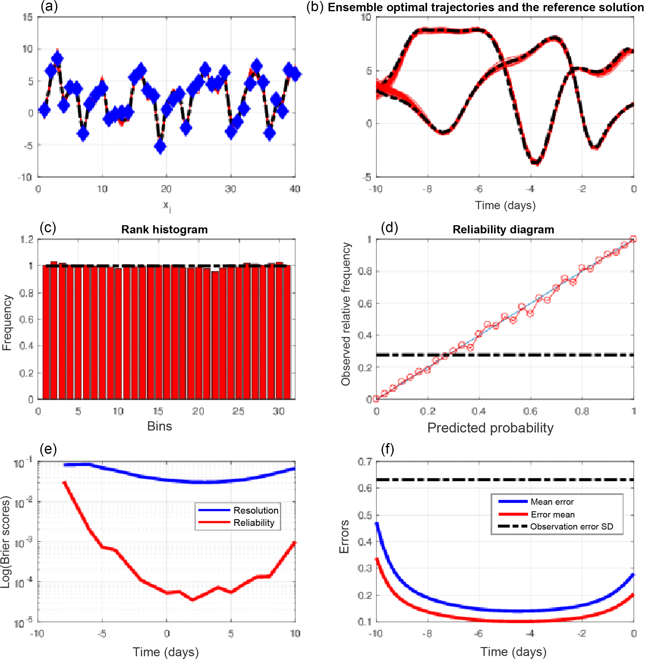
Figure 3 Same as Fig. 1, for quasi-static variational assimilations, with an increase in the length of the successive assimilation windows by 1 day. All scores are computed for the ensembles obtained from the final minimizations performed over the whole 10-day assimilation windows. The reliability diagram is relative to the event $\mathcal{E}=\mathit{\{}\mathit{x}<\mathrm{0.94}\mathit{\}}$, which occurs with frequency 0.29 (dashed–dotted horizontal curve).

The improvement over Fig. 1 is obvious. The spread of the minimizing solutions (top two panels) is much smaller, the rank histogram (middle left) is almost perfectly flat, the reliability diagram (middle right) is much closer to the diagonal, and both Brier scores (bottom left) have decreased. The estimation error (bottom right) is now, as it must, well below the observational error. The error in the ensemble mean (red curve) is now 0.1 at the middle point of the assimilation window, against 0.2 in Fig. I-4, relative to assimilations over 5-day windows (without QSVA). This improvement must be due to the fact that more observations, distributed over a longer assimilation window, have been used. In particular, as discussed in Bocquet and Sakov (2014), observations at the beginning and the end of the assimilation window must reduce the uncertainty in respectively the stable and unstable modes of the system. The rank histogram is also flatter than in the corresponding Fig. I-5. That must be due mostly to the larger validating sample.

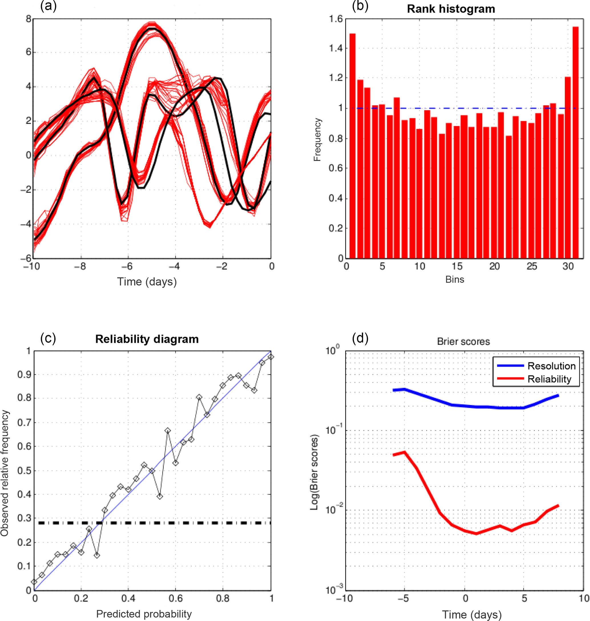
Figure 4, which is again in the same format as Figs. 1 and 3, is relative to an 18-day QSVA (with still an increment of 1 day between successive assimilation windows). It confirms the previous conclusions. The estimation error and both components of the Brier score are reduced even further.

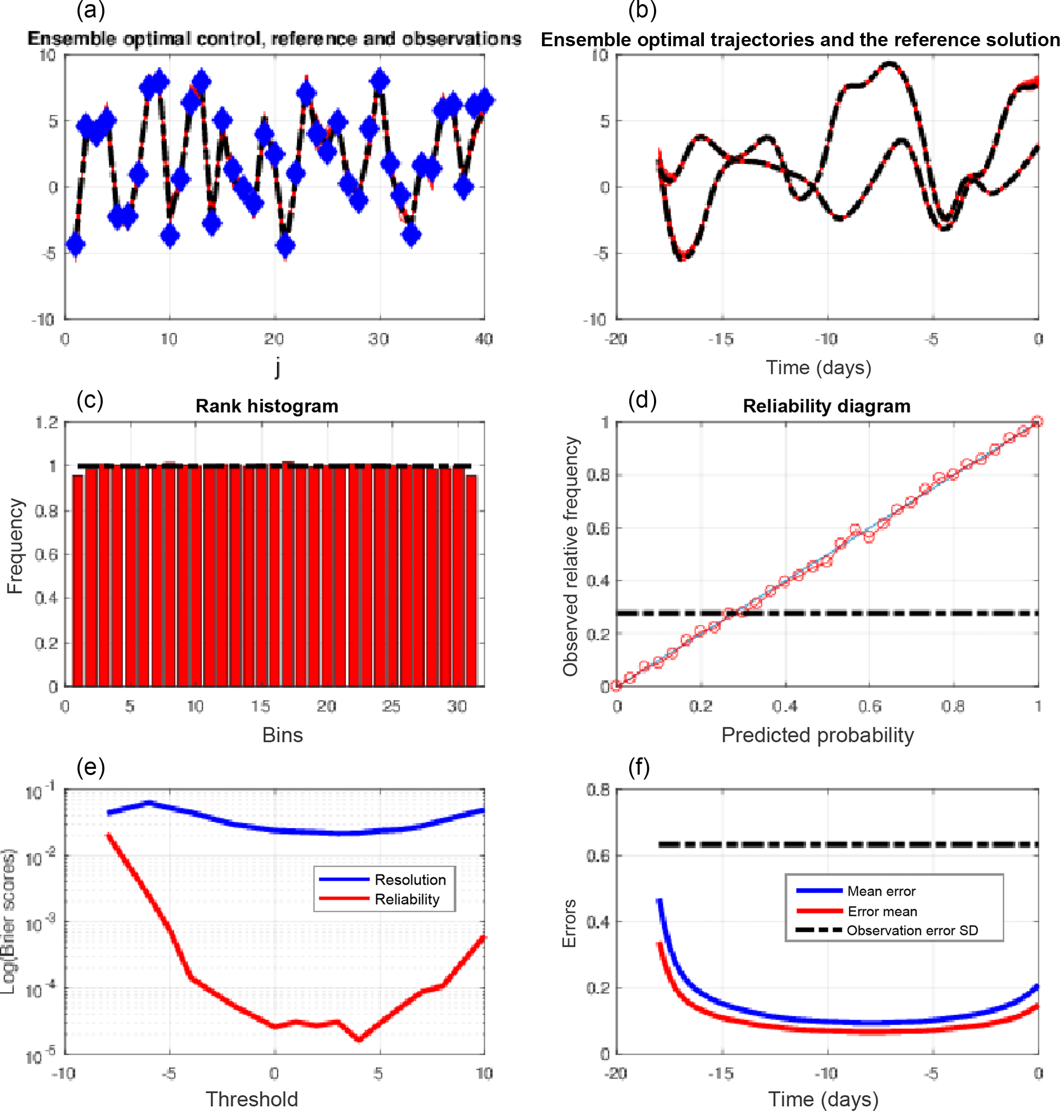
Figure 4 Same as Fig. 3, for quasi-static variational assimilations performed over 18-day assimilation windows, with an increase in the length of the successive assimilation windows by 1 day. The reliability diagram is for the event $\mathcal{E}=\mathit{\{}\mathit{x}<\mathrm{0.94}\mathit{\}}$, which occurs with frequency 0.29 (dashed–dotted horizontal curve).

All these results show that ensemble variational assimilation is successful, if implemented with QSVA, over long assimilation windows for which the tangent linear approximation is expected to fail. EnsVAR produces ensembles with a high degree of statistical reliability. In addition, the accuracy of the estimated ensembles, as measured by resolution or by the error in the ensemble mean, is improved when the length of the assimilation window is increased.

It can be noted that, if EnsVAR is successful in non-linear situations, it is not because of a possible intrinsically non-linear character. Minimization of an objective function of form (I-3) is a priori valid for statistical estimation only in a linear situation. The success of EnsVAR probably results from the fact that, through QSVA, it is capable of maintaining the current estimate of the flow within the ever-narrower region of state space in which the tangent linear approximation is valid. If the temporal density of the observations became so small, or alternatively if the dynamics of the observed system became so non-linear that it would not be possible to jump from one set of observations to the next one within a linear approximation, EnsVAR would probably fail. This point will deserve further study.

There is actually no reason to expect any strict link between the validity of the tangent linear approximation and the possible statistical reliability of minimizing solutions that lie within that approximation (not to speak of their Bayesianity). As already said, one can expect the a posteriori Bayesian probability distribution to be concentrated for long assimilation windows on a folded non-linear subset in state space. The bimodality of the histogram in Fig. 2 has been interpreted as separating the minimizations that lead to the absolute minimum of the objective function (left mode) from those that lead to a secondary minimum (right mode). This suggests, without resorting to QSVA, retaining only those minimizations corresponding to the left mode of the histogram. This of course requires, if one wants to obtain ensembles with dimension N_ens, a larger number of minimizations (even if there is of course no need to continue until convergence minimizations which show at an early stage that they will lead to the right mode of the histogram).

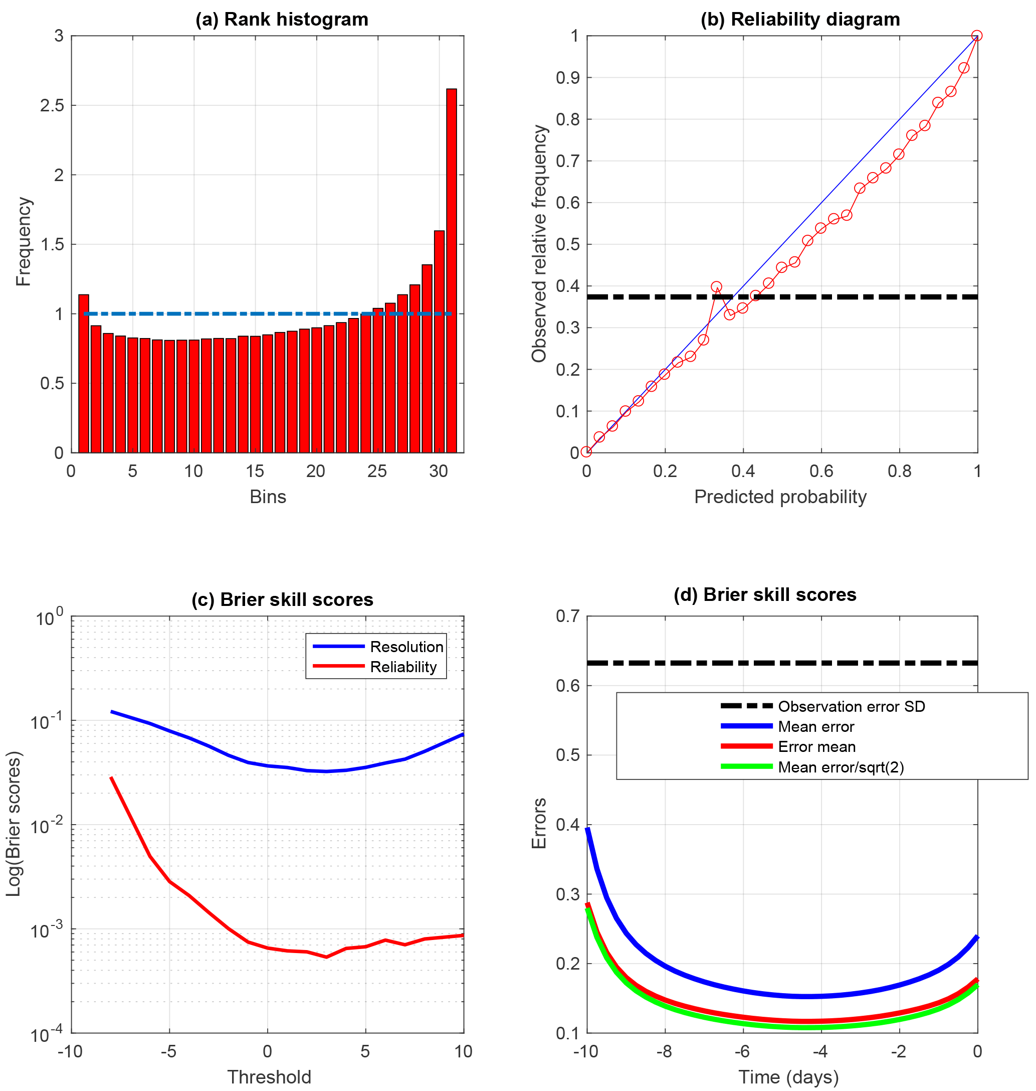
Figure 5 Same as the lower four panels of Fig. 1, restricted to minimizations that lead to the absolute minimum of the objective function (I-9), as identified from the value of the minimum itself (see Fig. 2). The diagnostics have been computed on 1443 realizations. The reliability diagram (b) is relative to the event $\mathcal{E}=\mathit{\{}\mathit{x}<\mathrm{0.33}\mathit{\}}$ , which occurs with frequency 0.38. In panel (d), which shows the RMS estimation errors along the assimilation window, the green curve has been obtained by dividing the values on the blue curve by a factor $\sqrt{\mathrm{2}}$.

This has been done on a set of N_win=1443 realizations (and over 10-day assimilation windows). The results are shown in Fig. 5, which presents the same diagnostics as those shown in the lower four panels of Fig. 1. The histogram (top-left panel) shows a distinct bias towards low values of the variable x, associated with a distinct underdispersion. This is confirmed by the reduced centred random variable (RCRV), which has positive mean 0.25 and standard deviation 1.29. It is also confirmed by the reliability diagram (top right), which lies below the diagonal, and the error curves (bottom right), where the ratio between the errors in the individual minimizations and in the mean of the ensembles is less than $\sqrt{\mathrm{2}}$. The former is qualitatively consistent with a bias towards low values of x, and the latter with both a bias and an underdispersion. Finally, concerning the Brier score (bottom left), it is seen that the reliability component is degraded with respect to QSVA (the resolution component, on the other hand, is not significantly modified).

Clearly, this procedure is a failure as far as reliability is concerned. But it can also be noted that the errors (bottom-right panel) are smaller than those of Fig. 3, especially at both extremities of the assimilation window. The errors in the individual minimizations (blue curve) are 0.395 and 0.24 at the beginning and end of the assimilation window (against 0.47 and 0.28 respectively in Fig. 3). As for the errors in the ensemble means (red curves), they are 0.28 and 0.175 at the beginning and end of the window (against 0.33 and 0.2 in Fig. 3). There is less difference at the middle of the window.

Judging from the above results, restricting the ensembles to minimizations that lead to the absolute minimum of the objective function degrades reliability, but improves to some extent the quadratic fit to reality. Now, the Bayesian expectation 𝔼(x|z) is the deterministic function of the data vector z that minimizes the error variance on the state vector x. Should the present results be confirmed, they would constitute an a contrario proof that QSVA, although it produces ensembles that possess high reliability, is not Bayesian.

3 Comparison with ensemble Kalman filter and particle filter

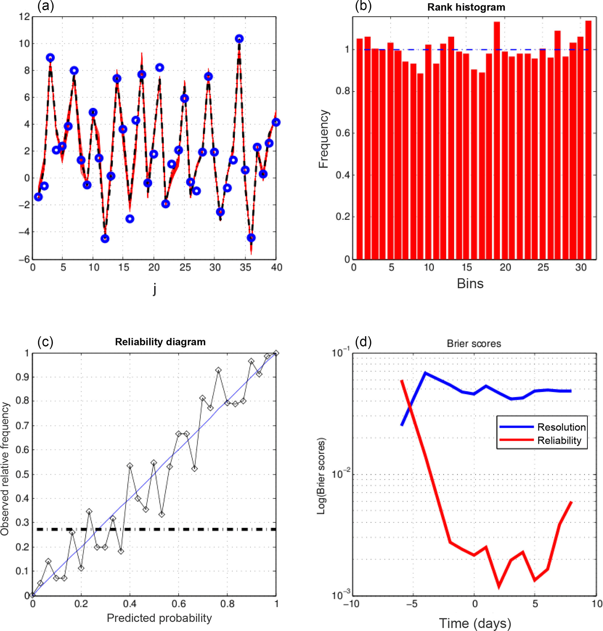
Figure 6 Further diagnostics of 10-day ensemble assimilations performed with QSVA EnsVAR. All diagnostics are performed at the end of the assimilation windows. (a) Truth (dashed black curve), observations (blue dots), and minimizing solutions (red curves), as functions of the spatial coordinate, at the end of one assimilation window. (b) Rank histogram for the variable x over all grid points and ensemble assimilations. (c) Reliability diagram for the event $\mathcal{E}=\mathit{\{}\mathit{x}<\mathrm{0.94}\mathit{\}}$, which occurs with frequency 0.29 (dashed–dotted horizontal curve), built over all grid points and ensemble assimilations. (d) Components of the Brier score (same format as in Fig. 1).

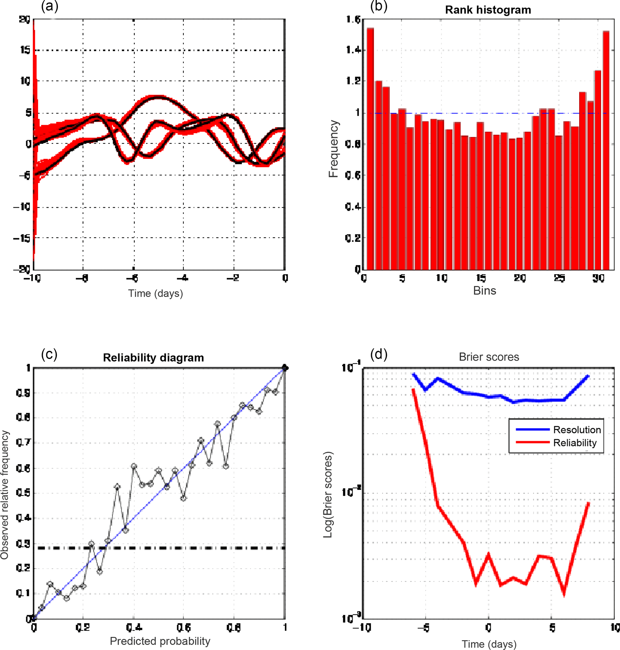
Figure 7 Diagnostics for assimilations performed with EnKF. (a) Temporal evolution, for one realization, of the truth at three grid points (black curves) and of the 30 corresponding ensemble solutions at the same points (red curves). The other three panels are in the same format as in Fig. 6 (and, as in Fig. 6, show diagnostics performed at the final time of the assimilation windows).

Figure 8 Same as Fig. 7, for assimilations performed with PF.

As in Part 1, we compare the results produced by EnsVAR with those produced by ensemble Kalman filter (EnKF) and particle filter (PF). Figures 6, 7, and 8 show the results obtained at the final time of 10-day assimilations performed with respectively QSVA EnsVAR, EnKF, and PF. The algorithms used for EnKF and PF are the same as in Part 1. Except for the top-left panel of Fig. 6, the format of the figures is the same as the format of Figs. 9–11 of Part 1. The top-left panel of Fig. 6, where the quantity on the horizontal axis is the spatial coordinate, shows the same diagnostics as the top-left panels of Figs. 3 and 4, but for the final time of an assimilation window. It is again seen that the dispersion of the minimizing ensemble solutions is small. The top-left panels of Figs. 7 and 8 show also the dispersion of the minimizing solutions for one assimilation window, but as a function of time along the window. The dispersion is small for EnKF, but distinctly larger for PF. The other panels show on all three figures diagnostics at the end of the assimilations. Concerning the rank histogram (top-right panels), it is noisy for EnsVAR, but does not show otherwise any sign of dissymmetry or inadequate spread. This is similar to what was observed in Part 1 at the end of 5 days of assimilation (Fig. I-9). On the other hand, the histograms for EnKF and PF, in addition to being noisy, and again as in Part 1 (Figs. I-10 and I-11), have a distinct U shape, which shows that the ensembles (although individually dispersed as shown by the top-left panels) tend to miss their target. Concerning the reliability diagrams (bottom-left panels), it is difficult to see visually any significant difference between the three algorithms. The Brier scores (bottom-right panels) show similar performance for EnsVAR and EnKF, but distinctly poorer performance for PF. This again is similar to what was observed in Part 1.

Similar results have been obtained, with the same conclusions, for longer assimilation periods (not shown).

EnsVAR shows therefore a slight advantage over EnKF and a more distinct advantage over PF. This conclusion is however to be taken with some caution and will be further discussed in the concluding section of the paper.

4 Weak-constraint assimilation

We present in this section the results of experiments that have been performed in the weak-constraint case when the deterministic model (I-6) is no longer considered as being exact. Following a standard approach, we now assume that the truth is governed by the equation

$$\begin{array}{}\text{(1)}& {\mathit{x}}_{k+\mathrm{1}}=\mathfrak{M}\left({\mathit{x}}_k\right)+{\mathit{b}}_k,\end{array}$$

where b_k is a white-in-time-and-space stochastic noise with probability distribution 𝒩(0,Q_k) at time k.

A typical experiment is as follows. A reference truth ${\mathit{x}}_k^{\mathrm{r}},k=\mathrm{0},\mathrm{\cdots },K$ is created using Eq. (1) for a particular realization of the noise b_k. Noisy observations y_k are extracted from that reference truth in the same way as in Part 1 (Eq. I-7). The data to be used in order to reconstruct the whole sequence of states ${\mathit{x}}_k^{\mathrm{r}}$ now consist of the observations y_k and of the a priori estimates ${\mathit{w}}_k=\mathbb{E}\left({\mathit{b}}_k\right)=\mathrm{0}$ of the noise b_k. The general expression (I-3) for the objective function to be minimized then takes the standard weak-constraint form

$$\begin{array}{ll}\text{(2)}& {\displaystyle }& {\displaystyle }\mathcal{J}({\mathit{\xi }}_{\mathrm{0}},{\mathit{\eta }}_{\mathrm{0}},{\mathit{\eta }}_{\mathrm{1}},\mathrm{\cdots },{\mathit{\eta }}_{K-\mathrm{1}})={\displaystyle }& {\displaystyle \frac{\mathrm{1}}{\mathrm{2}}}\sum _{k=\mathrm{0}}^K{\left[{\mathbf{H}}_k{\mathit{\xi }}_k-{\mathit{y}}_k\right]}^T{\mathbf{R}}_k^{-\mathrm{1}}\left[{\mathbf{H}}_k{\mathit{\xi }}_k-{\mathit{y}}_k\right]+{\displaystyle \frac{\mathrm{1}}{\mathrm{2}}}\sum _{k=\mathrm{0}}^{K-\mathrm{1}}{\mathit{\eta }}_k^T{\mathbf{Q}}_k^{-\mathrm{1}}{\mathit{\eta }}_k\end{array}$$

subject to

$$\begin{array}{}\text{(3)}& {\mathit{\xi }}_{k+\mathrm{1}}=\mathfrak{M}\left({\mathit{\xi }}_k\right)+{\mathit{\eta }}_k,k=\mathrm{0},\mathrm{\cdots },K-\mathrm{1}.\end{array}$$

Implementation of ensemble variational assimilation as studied here requires the perturbation of both the observations y_k and the estimates w_k according to their own error probability distribution. This leads to the minimization of objective functions of the form

$$\begin{array}{ll}{\displaystyle }& {\displaystyle }{\mathcal{J}}^{\mathrm{iens}}({\mathit{\xi }}_{\mathrm{0}},{\mathit{\eta }}_{\mathrm{0}},{\mathit{\eta }}_{\mathrm{1}},\mathrm{\cdots },{\mathit{\eta }}_{K-\mathrm{1}})=\\ \text{(4)}& {\displaystyle }& {\displaystyle \frac{\mathrm{1}}{\mathrm{2}}}\sum _{k=\mathrm{0}}^K{\left[{\mathbf{H}}_k{\mathit{\xi }}_k-({\mathit{y}}_k^{\mathrm{iens}}{)}^{\prime }\right]}^T{\mathbf{R}}_k^{-\mathrm{1}}\left[{\mathbf{H}}_k{\mathit{\xi }}_k-({\mathit{y}}_k^{\mathrm{iens}}{)}^{\prime }\right]+{\displaystyle }& {\displaystyle \frac{\mathrm{1}}{\mathrm{2}}}\sum _{k=\mathrm{0}}^{K-\mathrm{1}}{\left[{\mathit{\eta }}_k-({\mathit{w}}_k^{\mathrm{iens}}{)}^{\prime }\right]}^T{\mathbf{Q}}_k^{-\mathrm{1}}\left[{\mathit{\eta }}_k-({\mathit{w}}_k^{\mathrm{iens}}{)}^{\prime }\right]\end{array}$$

subject to condition (3).

In Eq. (4), $({\mathit{y}}_k^{\mathrm{iens}}{)}^{\prime }$ is obtained, as in Eq. (I-8), by perturbing the observation y_k, while $({\mathit{w}}_k^{\mathrm{iens}}{)}^{\prime }\sim \mathcal{N}(\mathbf{0},{\mathbf{Q}}_k)$ is the perturbation around w_k=0. As done above (and in Part 1) for the observational error, we do not consider the possibility that the statistical properties of the model error may be imperfectly known.

As previously, for given reference solution ${\mathit{x}}_k^{\mathrm{r}}$ and observations y_k, N_ens minimizations of objective functions of form (4) are performed with independent perturbations on y_k and w_k. This is repeated on N_win assimilation windows, with different ${\mathit{x}}_k^{\mathrm{r}}$ and observations y_k. N_ens will always be equal, as before, to 30. N_win will depend on the experiment.

The experiments have again been performed with the Lorenz-96 model (Eq. I-12). Experiments performed with a linearized version of the model have produced results (not shown) that are entirely consistent with the theory of the BLUE, within a numerical uncertainty which is similar to what has been observed in Part 1.

The covariance matrix Q_k of the stochastic noise has been taken equal to qI, where q is a positive scalar. Tests (not shown) have been made on the predictability associated with the different values of q. The value q=0.1, which corresponds to a predictability time of about 10 days, is used in the sequel.

The experimental procedure is otherwise the same as before. In particular, the complete state vector is observed every 0.5 days, with the observations being affected with uncorrelated unbiased Gaussian errors with the same variance σ=0.63 as in the strong-constraint case.

The first conclusion that has been obtained is that QSVA is no longer necessary for achieving the minimization, at least up to assimilation windows of length 18 days (the largest value that has been tried). Clearly the presence of the additional noise penalty term in Eq. (4) has a regularizing effect which acts as a smoother of the objective function variations. This is in agreement with results already obtained by Fisher et al. (2005) in a study of weak-constraint variational assimilation.

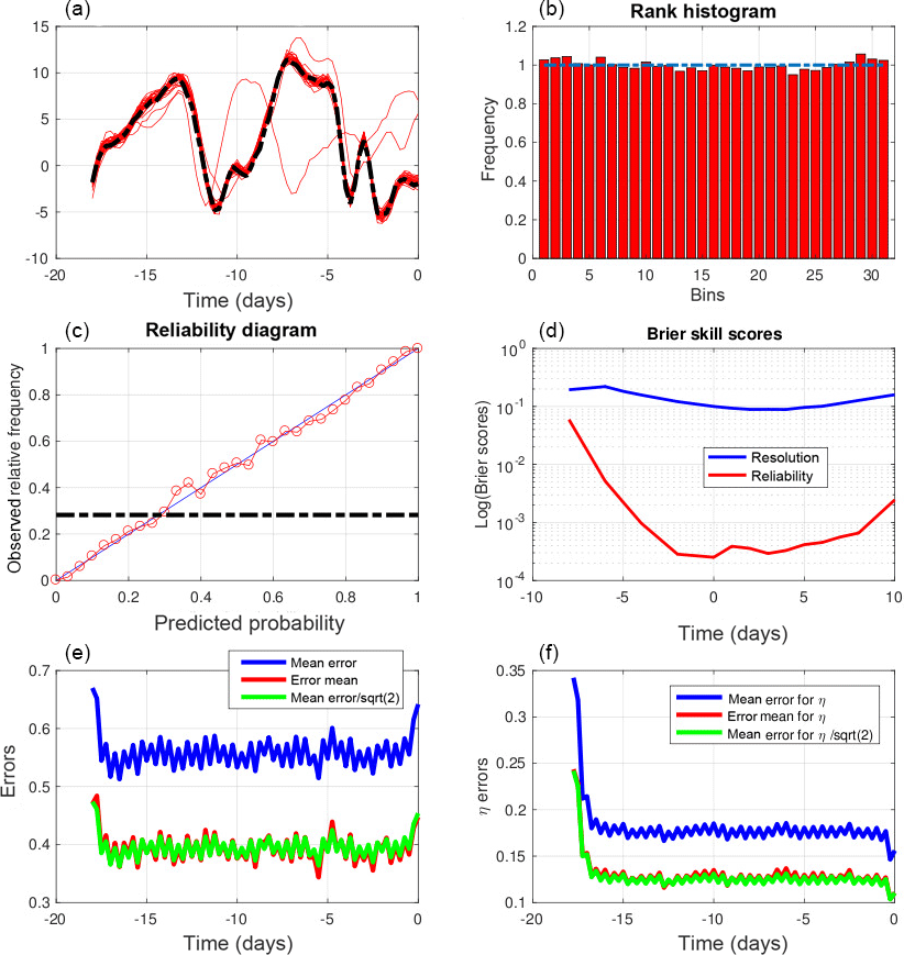
Figure 9 Diagnostics of weak-constraint variational assimilations performed over 18-day assimilation windows. (a) Truth (dashed curves) and minimizing solutions (red curves) as functions of time at one grid point over one assimilation window. (b) Rank histogram for the variable x over all grid points and ensemble assimilations. (c) Reliability diagram for the event $\mathcal{E}=\mathit{\{}x>\mathrm{1.02}\mathit{\}}$, which occurs with frequency 0.27 (dashed–dotted horizontal curve), built over all grid points and ensemble assimilations. (d) Components of the Brier score (same format as in the bottom-left panel of Fig. 1). (e, f) RMS estimation error on the state variable x and on the model noise b (e and f respectively), as functions of time along the assimilation windows. Blue curves: average RMS error in the individual minimizations. Red curves: average RMS error in the mean of the ensembles. The green curves are in the ratio $\mathrm{1}/\sqrt{\mathrm{2}}$ to the blue curves.

Figure 9 shows the results obtained over 18-day assimilation windows (and, because of computational cost, only N_win=1200 realizations). The figure is to be compared with Fig. 4, relative to 18-day strong-constraint variational assimilations. The top-left panel, relative to one particular realization, shows the temporal evolution, over the assimilation window and at a particular grid point, of the truth and of the corresponding 30 minimizing solutions. It is seen that, if most of the latter closely follow the former, there are nevertheless a few outliers (two solutions out of 30). In view of what has already been said, these outliers must correspond to secondary minima of the objective function (thus showing departure from strict linearity). The rank histogram (top right), the reliability diagram (middle left), and the Brier scores (middle right) show overall good performance, although not as good as in the strong-constraint case. In particular, both components of the Brier score are larger than their counterparts in Fig. 4 (bottom-left panel).

The bottom panels of Fig. 9 show the RMS estimation error on the state variable x_k and on the model noise b_k (left and right panels respectively), as functions of time along the assimilation windows. In addition to the average RMS error in the individual minimizations (blue curves) and in the mean of the ensembles (red curves), the green curves (as in the bottom-right panel of Fig. 5) are in the ratio $\mathrm{1}/\sqrt{\mathrm{2}}$ to the blue curves. The error is generally smaller than the standard deviation of the corresponding observation error (0.63 and 0.32 respectively). But it is actually larger in the individual minimizations at both ends of the assimilation window for the variable x_k and at the initial time of the window for the model noise b_k. The coincidence of the red and green curves indicates statistical reliability. The curves in both panels show oscillations with a half-a-day period, with minima at observation times for the x_k error and maxima for the b_k error. These oscillations are not visible in the individual minimizing solutions, nor in the mean of the ensembles (not shown), and become visible only on averages made over a large number of realizations. The origin of these oscillations can easily be understood. At observation times, the minimizing fields tend to fit closely the observations. In between observation times, on the contrary, the minimization adjusts the model noise so as to fit more closely the deterministic equation, with the consequence that the minimizing fields drift from the truth. These oscillations show up only because the temporal distribution of the observations is the same in all realizations of the assimilation. This interpretation is confirmed by Fig. 10, which shows the same diagnostics (without green curves) for weak-constraint assimilations over 5-day windows, with observations once every day. The top and bottom panels show errors in x_k and b_k respectively. The error in x_k is minimum at observation times, at which the error in b_k is maximum.

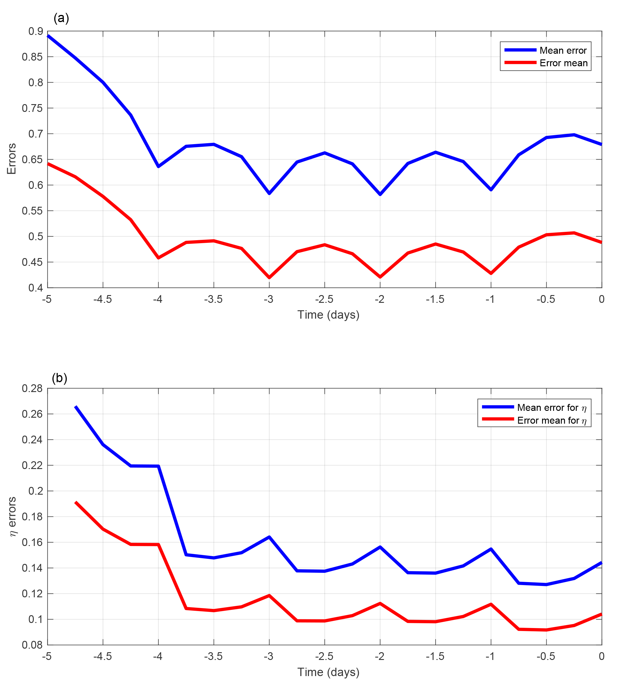
Figure 10 RMS estimation errors on the state variable x_k and on the model noise b_k (a and b respectively) for weak-constraint variational assimilations performed over 5-day windows, with observations at times $-\mathrm{5},-\mathrm{4},\mathrm{\dots },\mathrm{0}$.

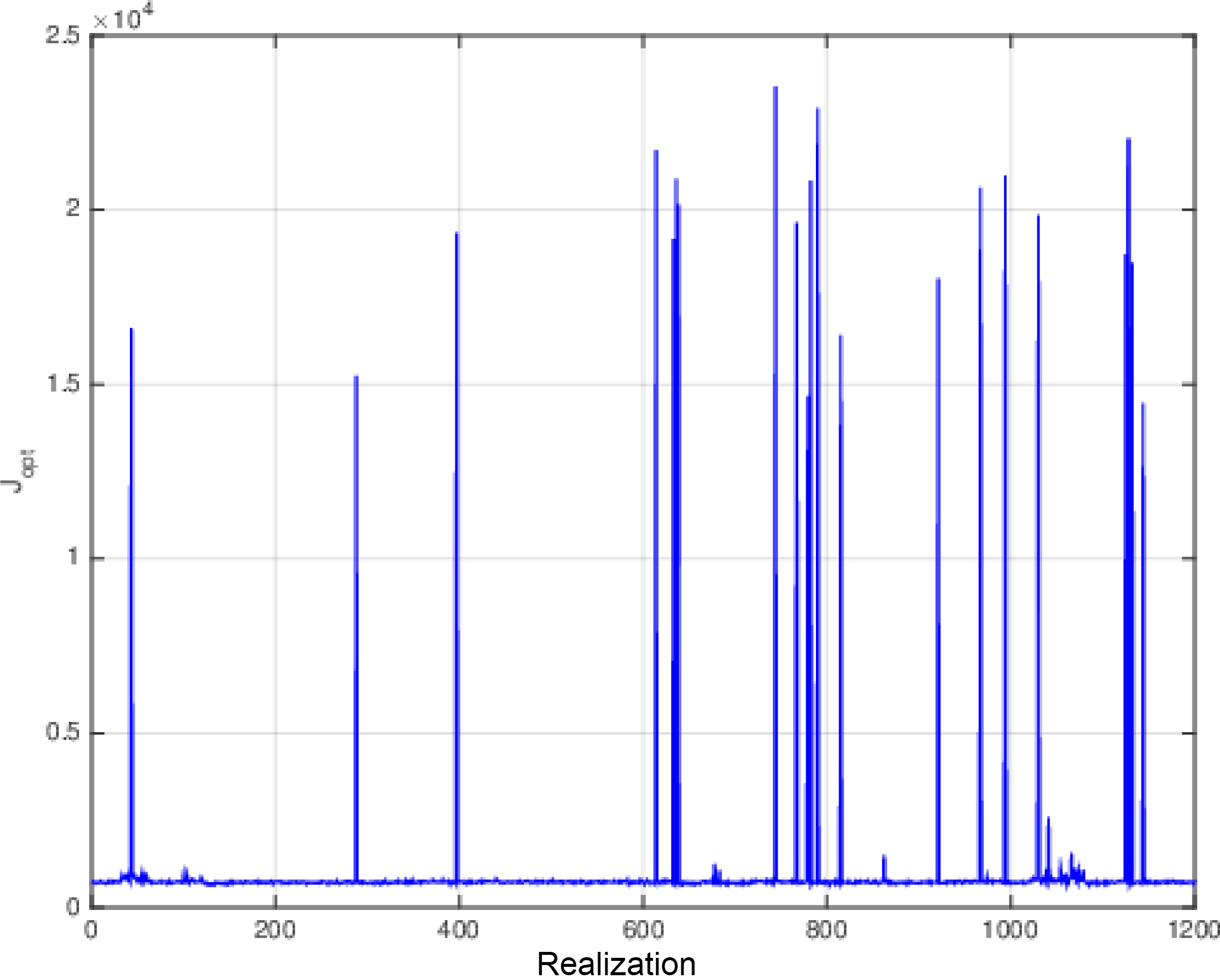
Figure 11 Values of (half) the minima of the objective function for all realizations of the weak-constraint assimilations over 18-day windows.

Figure 11, which is in the same format as Fig. I-7, shows the distribution of (half) the minima 𝒥_min of the objective functions. It is seen that, in superposition to a background of small minima, a number of very large values are present. These are interpreted as corresponding (as in Fig. I-7) to secondary minima of the objective function (associated, for instance, with the outliers of the top-left panel of Fig. 9). As concerns the theoretical χ² values, the number of observations of the variable x_k has now increased to $\mathrm{37}\times \mathrm{40}=\mathrm{1480}$. The use of weak constraint, which adds as many parameters to be determined as parameters to be adjusted in the objective function (2), does not modify the difference $p=m-n$. This leads for the expectation and standard deviation of 𝒥_min to the values $p/\mathrm{2}=\mathrm{720}$ and $\sqrt{p/\mathrm{2}}=\mathrm{26.8}$. The sample values in the background of small minima in Fig. 11 are respectively 727.45 and 25.51, in good agreement with the theoretical values, and with the interpretation that those small minima correspond to minimizing solutions that lie within the range of the tangent linear approximation.

These results show that, although there are clearly imperfections (minimizations occasionally lead to secondary minima), ensemble variational assimilation is on the whole very successful for weak-constraint assimilation.

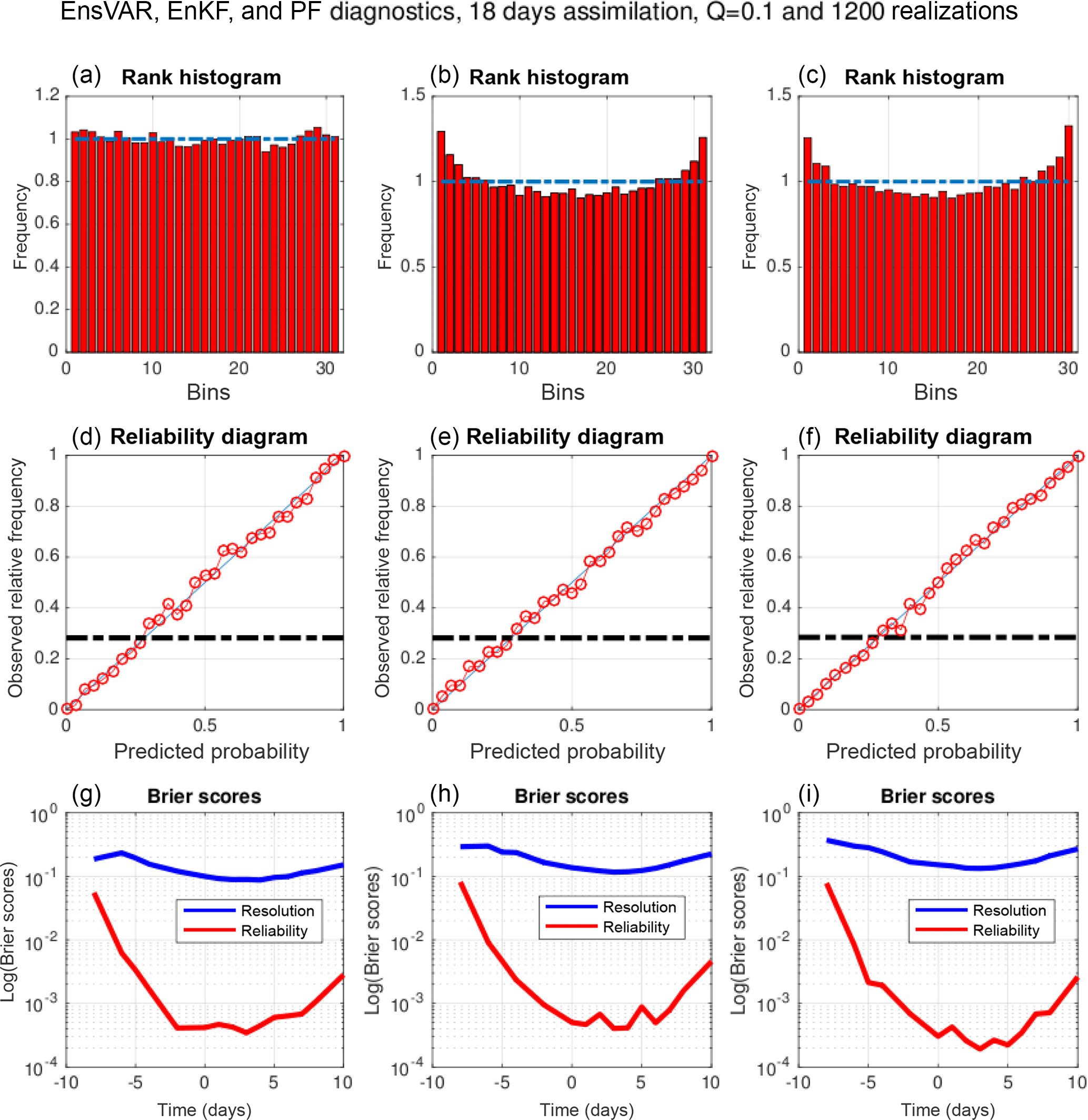
Figure 12 Compared performance of EnsVAR, EnKF, and PF (columns from left to right respectively) over the last 13 days of 18-day assimilation windows. (a, b, c) Rank histogram. (d, e, f) Reliability diagram for the event $\mathcal{E}=\mathit{\{}x>\mathrm{1.02}\mathit{\}}$, which occurs with frequency 0.27. (g, h, i) Reliability and resolution components of the Brier score for events x<τ as functions of the threshold τ.

Figure 12 shows the compared performance of EnsVAR, EnKF, and PF, evaluated over the last 13 days of the 18-day assimilation windows (this in order to eliminate the effects of the initialization of EnKF and PF). The experimental conditions for EnKF and PF are exactly the same as for EnsVAR (concerning the model noise, it has been added in the corresponding ensemble integrations in order to simulate the dispersion it would create in a real situation). The three columns correspond, from left to right, to EnsVAR, EnKF, and PF respectively. The rows show, from top to bottom, the rank histograms, the reliability diagrams, and the two components of the Brier score. The general performance of the three algorithms is similar. The only significant difference is seen on the rank histograms. The histogram for EnsVAR is much flatter than the other two histograms, which shows a distinct underdispersion of the ensembles. This is confirmed by the standard deviations of the RCRV diagnostic, which are equal to 1.02, 1.14, and 1.11 for EnsVAR, EnKF, and PF respectively.

5 Discussion and conclusions

The principle of ensemble variational assimilation (EnsVAR), which has been discussed in the two parts of this work, is very simple. Namely, perturb the data according to their own error probability distribution and, for each set of perturbed data, perform a standard variational assimilation. In the linear and additive Gaussian case, this produces a sample of independent realizations of the (Gaussian) Bayesian probability distribution for the state of the observed system, conditioned by the data.

The primary purpose of this work was to study EnsVAR as a probabilistic estimator in conditions (non-linearity and/or non-Gaussianity) where it cannot be expected to be an exact Bayesian estimator. Since the degree to which Bayesianity is achieved cannot be objectively evaluated, the weaker property of reliability has been evaluated instead. Standard scores, commonly used for evaluation of probabilistic prediction (rank histograms, reliability diagrams and associated Brier score, and in addition the reduced centred random variable) have been used to that end. The additional property of resolution, i.e. the degree to which the estimation system is capable of a priori distinguishing between different outcomes, has also been evaluated (resolution component of the Brier score, root-mean-square error in the mean of the ensembles). Indeed, one purpose of this work was to stress the importance, in the authors' minds, of evaluating ensemble assimilation systems as probabilistic estimators, particularly through the degree to which they achieve reliability and resolution.

The results presented in both parts of this paper show that EnsVAR is fundamentally successful in that, even in conditions where Bayesianity cannot be expected, it produces ensembles which possess a high degree of statistical reliability. Actually, the numerical scores for reliability that have been used are often as good, if not better, in situations where Bayesianity cannot be expected to hold than in situations where it holds. Better scores can be explained in the present situation only by better numerical conditioning. The resolution, as measured by the RMS error in the mean of the ensembles, or by the resolution component of the standard Brier score, is also high.

In non-linear strong-constraint cases, EnsVAR has been successful here only through the use of quasi-static variational assimilation, which significantly increases its numerical cost. However, in the weak-constraint case, QSVA has not been necessary, providing new evidence as to the favourable effect, on numerical efficiency of assimilation, of introducing a weak constraint. At the same time, the comparison of the results shown in the right bottom panels of Figs. 3 and 5 shows that EnsVAR, even when it has as high a degree of reliability as in purely linear and Gaussian situations, is not Bayesian.

Comparison with two other standard ensemble assimilation filters, namely ensemble Kalman filter and particle filter, made at constant ensemble size, shows a superior or equal performance for EnsVAR, at least as concerns the dispersion of the ensembles.

Our comparison is of course far from being complete. As already said, there exist many variants of both the EnKF and the PF, and EnsVAR has been compared here, for each of those two classes of algorithms, with only one of those variants. Several of these have been studied by Bocquet and Sakov (2013), Goodliff et al. (2015), and Carrassi et al. (2017), with however less emphasis than here on their performance as probabilistic estimators. A close comparison with these works would certainly be very instructive.

If a code for variational assimilation is available, EnsVAR is very easy (if costly) to implement. It possesses the advantages and disadvantages of standard variational assimilation. The advantages are the easy propagation of information both forward and backward in time (smoothing) and easy introduction of observations of new types and of temporal correlations between data errors. What is usually considered to be a major disadvantage of variational assimilation is the need for developing and maintaining an adjoint code. Concerning that point, it must however be stressed that algorithms are being developed which might avoid the need for adjoints while keeping most of the advantages of variational assimilation.

EnsVAR, as it has been implemented here, is very costly in that it requires a very large number of iterative minimizations. The comparison with EnKF and PF, which has been made here at constant ensemble size, might have led to different conclusions if it had been made at for example constant computing cost. In addition, the particular versions of EnKF and PF that have been used here may not be, among the many versions that exist for both algorithms, the most efficient ones for the problem considered here. In particular, concerning the EnKF, a deterministic version could be used instead of the stochastic version that has been used here. On the other hand, many possibilities exist for reducing the cost or at least the clock time of EnsVAR, through simple parallelization or through use of the results of the first minimizations to speed up the following ones. The rapid development of algorithmic science makes it difficult to draw definitive conclusions at this stage as to the compared cost of various methods for ensemble assimilation.

EnsVAR, at it has been presented here, is almost uniquely defined on the basis of its principle. It has been necessary to introduce only one arbitrary parameter for the experiments that have been described, namely the temporal increment (1 day) between successive assimilation windows in QSVA. Everything else is unambiguously defined once the principle of EnsVAR has been stated. This may of course not remain true in the future, but is certainly a distinct advantage to start with. On the other hand, EnsVAR, like actually the EnKF and the PF, is largely empirical, with the consequence that, should difficulties arise, conceptual guidelines may be missing to solve these difficulties. The only thing that can be said at this stage is that EnsVAR is successful in non-linear situations probably because it keeps the estimation problem within the basin of attraction of the absolute minimum of the objective function to be minimized.

One can also remark that EnsVAR, in the form in which it has been implemented here, and contrary to EnKF and PF, produces an ensemble of totally independent realizations of a same probability distribution. It is difficult to say if that can be considered as a distinct advantage, but it is certainly not a disadvantage.

The problem of cycling EnsVAR for one assimilation window to the next one has not been considered here. It has been studied to some extent by Bocquet and Sakov (2013, 2014) in the context of another form of ensemble assimilation. The general questions that arise range from the simplest one (is cycling necessary at all, or can one simply proceed by implementing EnsVAR over successive, possibly overlapping, windows?) to the question of carrying a background ensemble from one window to the next, together with an associated error covariance matrix. In the latter case, the difficulties associated with localization and inflation, which have significantly complicated the development of EnKF, might arise again. One interesting possibility is to use the ideas of assimilation in the unstable subspace (AUS), advocated by Trevisan and colleagues (see, Trevisan et al., 2010, and Palatella et al., 2013), in which the control variable of the assimilation is restricted to the modes of the system that have been unstable in the recent past, where the uncertainty in the state of the system is most likely to be concentrated. This approach is actively studied at present (see e.g. Bocquet and Carrassi, 2017).

EnsVAR has been implemented here on a small-dimension system. It is operationally running at both ECMWF and Météo-France to specify initial conditions for the ensemble forecast and to construct the background error covariance matrix for the variational assimilation. It has not been systematically evaluated as a probabilistic estimator on a physically realistic large-dimensional model. It has also to be compared with other ensemble assimilation methods, in terms of both intrinsic quality of the results and of cost efficiency. In addition to the many variants of ensemble Kalman filter and particle filter, one can mention the Metropolis–Hastings algorithm, which, as already said in the introduction of Part 1, possesses itself many variants. It has been used for many applications, most of which, if not all, are however relative to problems with small dimensions. It would be extremely interesting to study the performance in problems of assimilation for geophysical fluids. More recently, and in the continuation of Bardsley (2012), Bardsley et al. (2014) have proposed what they call the randomize-then-optimize (RTO) algorithm. This defines a theoretical improvement on EnsVAR, based on an appropriate use of the Jacobian of the data operator. But, as for EnsVAR itself, the question of whether it can be implemented on large-dimension models (see e.g. Liu et al., 2017) is still open. Systematic comparison of the performances of the many algorithms that now exist for ensemble assimilation, in particular in terms of their capability of achieving Bayesian estimation, will certainly be very instructive.