Sensitivity analysis with respect to observations in variational data assimilation for parameter estimation

The problem of variational data assimilation for a nonlinear evolution model is formulated as an optimal control problem to find unknown parameters of the model. The observation data, and hence the optimal solution, may contain uncertainties. A response function is considered as a functional of the optimal solution after assimilation. Based on the second-order adjoint techniques, the sensitivity of the response function to the observation data is studied. The gradient of the response function is related to the solution of a nonstandard problem involving the coupled system of direct and adjoint equations. The nonstandard problem is studied, based on the Hessian of the original cost function. An algorithm to compute the gradient of the response function with respect to observations is presented. A numerical example is given for the variational data assimilation problem related to sea surface temperature for the Baltic Sea thermodynamics model.

1 Introduction

The methods of data assimilation have become an important tool for analysis of complex physical phenomena in various fields of science and technology. These methods allow us to combine mathematical models, data resulting from observations, and a priori information. The problems of variational data assimilation can be formulated as optimal control problems (e.g., Lions, 1968; Le Dimet and Talagrand, 1986) to find unknown model parameters, such as initial and/or boundary conditions, right-hand sides in the model equations (forcing terms), and distributed coefficients, based on minimization of the cost function related to observations. A necessary optimality condition reduces an optimal control problem to an optimality system which involves the model equations, the adjoint problem, and input data functions. The optimal solution depends on the observation data, and for future forecasts it is very important to study the sensitivity of the optimal solution with respect to observation errors (Baker and Daley, 2000).

The necessary optimality condition is related to the gradient of the original cost function; thus, to study the sensitivity of the optimal solution, one should differentiate the optimality system with respect to observations. In this case, we come to the so-called second-order adjoint problem (Le Dimet et al., 2002). The first studies of sensitivity of the response functions after assimilation with the use of second-order adjoint were done by Le Dimet et al. (1997) for variational data assimilation problems aimed at restoration of initial condition, where sensitivity with respect to model parameters was considered. The equations of the forecast sensitivity to observations in a four-dimensional (4D-Var) data assimilation were derived by Daescu (2008). Based on these results, a practical computational approach was given by Cioaca et al. (2013) to quantify the effect of observations in 4D-Var data assimilation.

The issue of sensitivity is related to the statistical properties of the optimal solution (see Gejadze et al., 2008, 2011, 2013; Shutyaev et al., 2012). General sensitivity analysis in variational data assimilation with respect to observations for a nonlinear dynamic model was given by Shutyaev et al. (2017) to control the initial-value function. The dynamic formulation of the problem is important because it shows different implementation options (Gejadze et al., 2018).

This paper is based on the results of Shutyaev et al. (2017) and presents the sensitivity analysis with respect to observations in variational data assimilation aimed at restoration of unknown parameters of a dynamic model. We should mention the importance of the parameter estimation problem itself. A precise determination of the initial condition is very important in view of forecasting; however, the use of variational data assimilation is not limited to operational forecasting. In many domains (e.g., hydrology) the uncertainty in the parameters is more crucial than the uncertainty in the initial condition (e.g., White at al., 2003). In some problems the quantity of interest can be represented directly by the estimated parameters as controls. For example, in Agoshkov et al. (2015) the sea surface heat flux is estimated in order to understand its spatial and temporal variability. The problems of parameter estimation are common inverse problems considered in geophysics and in engineering applications (see Alifanov et al., 1996; Sun, 1994; Zhu and Navon, 1999; Storch et al., 2007). In the last years, interest in the parameter estimation using 4D-Var is rising (Bocquet, 2012; Schirber at al., 2013; Yuepeng et al., 2018; Agoshkov and Sheloput, 2017).

We consider a dynamic formulation of the variational data assimilation problem for parameter estimation in a continuous form, but the presented sensitivity analysis formulas with respect to observations do not follow from our previous results for the initial condition problem (Shutyaev et al., 2017) and constitute a novelty of this paper. Of course, the initial condition function may also be considered as a parameter; however, in our dynamic formulation we have two equations for the model: one equation for describing an evolution of the model operator (involving model parameters such as right-hand sides, coefficients, boundary conditions, etc.) and another equation is considered as an initial condition.

This paper is organized as follows. In Sect. 2, we give the statement of the variational data assimilation problem for a nonlinear evolution model to estimate the model parameters. In Sect. 3, sensitivity of the response function after assimilation with respect to observations is studied, and its gradient is related to the solution of a nonstandard problem. In Sect. 4 we derive an operator equation involving the Hessian to study the solvability of the nonstandard problem, and give an algorithm to compute the gradient of the response function. A proof-of-concept analytic example with a simple model is given in Sect. 5 to demonstrate how the sensitivity analysis algorithm works. Section 6 presents an application of the theory to the data assimilation problem for a sea thermodynamics model. Numerical examples are given in Sect. 7 for the Baltic Sea dynamics model. The main results are discussed in Sect. 8.

2 Statement of the problem

We consider the mathematical model of a physical process that is described by the evolution problem

$$\begin{array}{}\text{(1)}& \left\{\begin{array}{lll}{\displaystyle \frac{\partial \mathit{\phi }}{\partial t}}& =F(\mathit{\phi },\mathit{\lambda })+f,& t\in (\mathrm{0},T)\\ \mathit{\phi }{|}_{t=\mathrm{0}}& =u,& \end{array}\right.\end{array}$$

where the initial state u belongs to a Hilbert space X, φ=φ(t) is the unknown function belonging to $Y=L_{\mathrm{2}}(\mathrm{0},T;X)$ with the norm $\Vert \mathit{\phi }{\Vert }_Y=(\mathit{\phi },\mathit{\phi }{)}_Y^{\mathrm{1}/\mathrm{2}}=({\int }_{\mathrm{0}}^T\Vert \mathit{\phi }\left(t\right){\Vert }_X^{\mathrm{2}}\text{d}t{)}^{\mathrm{1}/\mathrm{2}}$, F is a nonlinear operator mapping Y×Y_p into Y, Y_p is a Hilbert space (space of control parameters, or control space), and f∈Y. Suppose that for a given $u\in X,f\in Y$, and λ∈Y_p, there exists a unique solution φ∈Y to Eq. (1) with $\frac{\partial \mathit{\phi }}{\partial t}\in Y$. The function λ is an unknown model parameter. Let us introduce the cost function

$$\begin{array}{ll}\text{(2)}& {\displaystyle }J\left(\mathit{\lambda }\right)=& {\displaystyle \frac{\mathrm{1}}{\mathrm{2}}}\left(V_{\mathrm{1}}\right(\mathit{\lambda }-{\mathit{\lambda }}_{\text{b}}),\mathit{\lambda }-{\mathit{\lambda }}_{\text{b}}{)}_{Y_{\text{p}}}{\displaystyle }& {\displaystyle }+{\displaystyle \frac{\mathrm{1}}{\mathrm{2}}}\left(V_{\mathrm{2}}\right(C\mathit{\phi }-{\mathit{\phi }}_{\text{obs}}),C\mathit{\phi }-{\mathit{\phi }}_{\text{obs}}{)}_{Y_{\text{obs}}},\end{array}$$

where λ_b∈Y_p is a prior (background) function, φ_obs∈Y_obs is a prescribed function (observational data), Y_obs is a Hilbert space (observation space), $C:Y\to Y_{\text{obs}}$ is a linear bounded observation operator, and $V_{\mathrm{1}}:Y_{\text{p}}\to Y_{\text{p}}$ and $V_{\mathrm{2}}:Y_{\text{obs}}\to Y_{\text{obs}}$ are symmetric positive definite bounded operators.

Let us consider the following data assimilation problem with the aim to estimate the parameter λ: for a given $u\in X,$ and f∈Y, find λ∈Y_p and φ∈Y such that they satisfy Eq. (1), and on the set of solutions to Eq. (1), the functional J(λ) takes the minimum value, i.e.,

$$\begin{array}{}\text{(3)}& \left\{\begin{array}{lll}{\displaystyle \frac{\partial \mathit{\phi }}{\partial t}}& =F(\mathit{\phi },\mathit{\lambda })+f,& t\in (\mathrm{0},T)\\ \mathit{\phi }{|}_{t=\mathrm{0}}& =u,& \\ J\left(\mathit{\lambda }\right)& =\underset{v\in Y_{\text{p}}}{inf}J\left(v\right).& \end{array}\right.\end{array}$$

We suppose that the solution of Eq. (3) exists. Let us note that the solvability of the parameter estimation problems (or identifiability) has been addressed, e.g., in Chavent (1983) and Navon (1998). To derive the optimality system, we assume the solution φ and the operator F(φ,λ) in Eqs. (1)–(2) are regular enough, and for v∈Y_p find the gradient of the functional J with respect to λ:

$$\begin{array}{ll}\text{(4)}& {\displaystyle }{J}^{\prime }\left(\mathit{\lambda }\right)v& {\displaystyle }=\left(V_{\mathrm{1}}\right(\mathit{\lambda }-{\mathit{\lambda }}_{\text{b}}),v{)}_{Y_{\text{p}}}+(V_{\mathrm{2}}(C\mathit{\phi }-{\mathit{\phi }}_{\text{obs}}),C\mathit{\varphi }{)}_{Y_{\text{obs}}}{\displaystyle }& {\displaystyle }=\left(V_{\mathrm{1}}\right(\mathit{\lambda }-{\mathit{\lambda }}_{\text{b}}),v{)}_{Y_{\text{p}}}+(C^{*}{V}_{\mathrm{2}}(C\mathit{\phi }-{\mathit{\phi }}_{\text{obs}}),\mathit{\varphi }{)}_Y,\end{array}$$

where ϕ is the solution to the problem:

$$\begin{array}{}\text{(5)}& \left\{\begin{array}{lll}{\displaystyle \frac{\partial \mathit{\varphi }}{\partial t}}& =& F_{\mathit{\phi }}^{\prime }(\mathit{\phi },\mathit{\lambda })\mathit{\varphi }+F_{\mathit{\lambda }}^{\prime }(\mathit{\phi },\mathit{\lambda })v,\\ \mathit{\varphi }{|}_{t=\mathrm{0}}& =& \mathrm{0}.\end{array}\right.\end{array}$$

Here $F_{\mathit{\phi }}^{\prime }(\mathit{\phi },\mathit{\lambda }):Y\to Y,F_{\mathit{\lambda }}^{\prime }(\mathit{\phi },\mathit{\lambda }):Y_{\text{p}}\to Y$ are the Fréchet derivatives of F (Marchuk et al., 1996) with respect to φ and λ, correspondingly, and C^* is the adjoint operator to C defined by $(C\mathit{\phi },\mathit{\psi }{)}_{Y_{\text{obs}}}=(\mathit{\phi },C^{*}\mathit{\psi }{)}_Y,\mathit{\phi }\in Y,\mathit{\psi }\in Y_{\text{obs}}$.

Let us consider the adjoint operator $\left(F_{\mathit{\phi }}^{\prime }\right(\mathit{\phi },\mathit{\lambda }){)}^{*}:Y\to Y$ and introduce the adjoint problem:

$$\begin{array}{}\text{(6)}& \left\{\begin{array}{lll}{\displaystyle \frac{\partial {\mathit{\phi }}^{*}}{\partial t}}+\left(F_{\mathit{\phi }}^{\prime }\right(\mathit{\phi },\mathit{\lambda }){)}^{*}{\mathit{\phi }}^{*}& =& C^{*}{V}_{\mathrm{2}}(C\mathit{\phi }-{\mathit{\phi }}_{\text{obs}}),\\ {\mathit{\phi }}^{*}{|}_{t=T}& =& \mathrm{0}.\end{array}\right.\end{array}$$

Then Eq. (4) with Eqs. (5) and (6) gives

$$\begin{array}{ll}\text{(7)}& {\displaystyle }{J}^{\prime }\left(\mathit{\lambda }\right)v& {\displaystyle }=\left(V_{\mathrm{1}}\right(\mathit{\lambda }-{\mathit{\lambda }}_{\text{b}}),v{)}_{Y_{\text{p}}}-({\mathit{\phi }}^{*},F_{\mathit{\lambda }}^{\prime }(\mathit{\phi },\mathit{\lambda })v{)}_Y{\displaystyle }& {\displaystyle }=\left(V_{\mathrm{1}}\right(\mathit{\lambda }-{\mathit{\lambda }}_{\text{b}}),v{)}_{Y_{\text{p}}}-(\left(F_{\mathit{\lambda }}^{\prime }\right(\mathit{\phi },\mathit{\lambda }){)}^{*}{\mathit{\phi }}^{*},v{)}_{Y_{\text{p}}},\end{array}$$

where $\left(F_{\mathit{\lambda }}^{\prime }\right(\mathit{\phi },\mathit{\lambda }){)}^{*}:Y\to Y_{\text{p}}$ is the adjoint operator to $F_{\mathit{\lambda }}^{\prime }(\mathit{\phi },\mathit{\lambda })$. Therefore, the gradient of J is defined by

$$J^{\prime }\left(\mathit{\lambda }\right)=V_{\mathrm{1}}(\mathit{\lambda }-{\mathit{\lambda }}_{\text{b}})-\left(F_{\mathit{\lambda }}^{\prime }\right(\mathit{\phi },\mathit{\lambda }){)}^{*}{\mathit{\phi }}^{*}.$$

From Eqs. (4)–(7) we get the optimality system (the necessary optimality conditions; Lions, 1968):

$$\begin{array}{}\text{(8)}& \left\{\begin{array}{lll}{\displaystyle \frac{\partial \mathit{\phi }}{\partial t}}& =F(\mathit{\phi },\mathit{\lambda })+f,& t\in (\mathrm{0},T),\\ \mathit{\phi }{|}_{t=\mathrm{0}}& =u,& \end{array}\right.\end{array}$$

$$\begin{array}{}\text{(9)}& \left\{\begin{array}{lll}{\displaystyle \frac{\partial {\mathit{\phi }}^{*}}{\partial t}}+\left(F_{\mathit{\phi }}^{\prime }\right(\mathit{\phi },\mathit{\lambda }){)}^{*}{\mathit{\phi }}^{*}& =& C^{*}{V}_{\mathrm{2}}(C\mathit{\phi }-{\mathit{\phi }}_{\text{obs}}),\\ {\mathit{\phi }}^{*}{|}_{t=T}& =& \mathrm{0},\end{array}\right.\end{array}$$

$$\begin{array}{}\text{(10)}& V_{\mathrm{1}}(\mathit{\lambda }-{\mathit{\lambda }}_{\text{b}})-\left(F_{\mathit{\lambda }}^{\prime }\right(\mathit{\phi },\mathit{\lambda }){)}^{*}{\mathit{\phi }}^{*}=\mathrm{0}.\end{array}$$

We assume that the system (Eqs. 8–10) has a unique solution. The system (Eqs. 8–10) may be considered as a generalized model 𝒜(U)=0 with the state variable $U=(\mathit{\phi },{\mathit{\phi }}^{*},\mathit{\lambda })$, and it contains information about observations. In what follows we study the problem of the sensitivity of functionals of the optimal solution to the observation data.

If the observation operator C is nonlinear, i.e., Cφ=C(φ), then the right-hand side of the adjoint equation (Eq. 9) contains $(C_{\mathit{\phi }}^{\prime }{)}^{*}$ instead of C^* and all the analysis presented below is similar.

3 Sensitivity of functionals after assimilation

In geophysical applications the observation data cannot be measured precisely; therefore, it is important to be able to estimate the impact of uncertainties in observations on the outputs of the model after assimilation.

Let us introduce a response function G(φ,λ), which is supposed to be a real-valued function and can be considered as a functional on Y×Y_p. We are interested in the sensitivity of G with respect to φ_obs, with φ and λ obtained from the optimality system (Eqs. 8–10). By definition, the sensitivity is defined by the gradient of G with respect to φ_obs:

$$\begin{array}{}\text{(11)}& {\displaystyle \frac{\text{d}G}{\text{d}{\mathit{\phi }}_{\text{obs}}}}={\displaystyle \frac{\partial G}{\partial \mathit{\phi }}}{\displaystyle \frac{\partial \mathit{\phi }}{\partial {\mathit{\phi }}_{\text{obs}}}}+{\displaystyle \frac{\partial G}{\partial \mathit{\lambda }}}{\displaystyle \frac{\partial \mathit{\lambda }}{\partial {\mathit{\phi }}_{\text{obs}}}}.\end{array}$$

If δφ_obs is a perturbation on φ_obs, we get from the optimality system:

$$\begin{array}{}\text{(12)}& \left\{\begin{array}{lll}{\displaystyle \frac{\partial \mathit{\delta }\mathit{\phi }}{\partial t}}& =& F_{\mathit{\phi }}^{\prime }(\mathit{\phi },\mathit{\lambda })\mathit{\delta }\mathit{\phi }+F_{\mathit{\lambda }}^{\prime }(\mathit{\phi },\mathit{\lambda })\mathit{\delta }\mathit{\lambda },\\ \mathit{\delta }\mathit{\phi }{|}_{t=\mathrm{0}}& =& \mathrm{0},\end{array}\right.\end{array}$$

$$\begin{array}{}\text{(13)}& \left\{\begin{array}{l}-{\displaystyle \frac{\partial \mathit{\delta }{\mathit{\phi }}^{*}}{\partial t}}-\left(F_{\mathit{\phi }}^{\prime }\right(\mathit{\phi },\mathit{\lambda }){)}^{*}\mathit{\delta }{\mathit{\phi }}^{*}-(F_{\mathit{\phi }\mathit{\phi }}^{\prime \prime }(\mathit{\phi },\mathit{\lambda })\mathit{\delta }\mathit{\phi }{)}^{*}{\mathit{\phi }}^{*}\\ =\left(F_{\mathit{\phi }\mathit{\lambda }}^{\prime \prime }\right(\mathit{\phi },\mathit{\lambda })\mathit{\delta }\mathit{\lambda }{)}^{*}{\mathit{\phi }}^{*}-C^{*}{V}_{\mathrm{2}}(C\mathit{\delta }\mathit{\phi }-\mathit{\delta }{\mathit{\phi }}_{\text{obs}}),\\ \mathit{\delta }{\mathit{\phi }}^{*}{|}_{t=T}=\mathrm{0},\end{array}\right.\end{array}$$

$$\begin{array}{ll}\text{(14)}& {\displaystyle }{V}_{\mathrm{1}}\mathit{\delta }\mathit{\lambda }& {\displaystyle }-\left(F_{\mathit{\lambda }\mathit{\phi }}^{\prime \prime }\right(\mathit{\phi },\mathit{\lambda })\mathit{\delta }\mathit{\phi }{)}^{*}{\mathit{\phi }}^{*}-(F_{\mathit{\lambda }\mathit{\lambda }}^{\prime \prime }(\mathit{\phi },\mathit{\lambda })\mathit{\delta }\mathit{\lambda }{)}^{*}{\mathit{\phi }}^{*}{\displaystyle }& {\displaystyle }-\left(F_{\mathit{\lambda }}^{\prime }\right(\mathit{\phi },\mathit{\lambda }){)}^{*}\mathit{\delta }{\mathit{\phi }}^{*}=\mathrm{0},\end{array}$$

and

$$\begin{array}{}\text{(15)}& {\left({\displaystyle \frac{\text{d}G}{\text{d}{\mathit{\phi }}_{\text{obs}}}},\mathit{\delta }{\mathit{\phi }}_{\text{obs}}\right)}_{Y_{\text{obs}}}={\left({\displaystyle \frac{\partial G}{\partial \mathit{\phi }}},\mathit{\delta }\mathit{\phi }\right)}_Y+{\left({\displaystyle \frac{\partial G}{\partial \mathit{\lambda }}},\mathit{\delta }\mathit{\lambda }\right)}_{Y_{\text{p}}},\end{array}$$

where δφ, δφ^*, and δλ are the Gâteaux derivatives of φ, φ^*, and λ in the direction δφ_obs (for example, $\mathit{\delta }\mathit{\phi }=\frac{\partial \mathit{\phi }}{\partial {\mathit{\phi }}_{\text{obs}}}\mathit{\delta }{\mathit{\phi }}_{\text{obs}}$).

To compute the gradient ${\mathrm{\nabla }}_{{\mathit{\phi }}_{\text{obs}}}G(\mathit{\phi },\mathit{\lambda })$, let us introduce three adjoint variables P₁∈Y, P₂∈Y, and P₃∈Y_p. By taking the inner product of Eq. (12) by P₁, Eq. (13) by P₂, and of Eq. (14) by P₃ and adding them,

$$\begin{array}{ll}{\displaystyle }& {\displaystyle }{\left({\displaystyle \frac{\partial \mathit{\delta }\mathit{\phi }}{\partial t}}-F_{\mathit{\phi }}^{\prime }(\mathit{\phi },\mathit{\lambda })\mathit{\delta }\mathit{\phi }-F_{\mathit{\lambda }}^{\prime }(\mathit{\phi },\mathit{\lambda })\mathit{\delta }\mathit{\lambda },P_{\mathrm{1}}\right)}_Y\\ {\displaystyle }& {\displaystyle }+\left(-{\displaystyle \frac{\partial \mathit{\delta }{\mathit{\phi }}^{*}}{\partial t}}-\left(F_{\mathit{\phi }}^{\prime }\right(\mathit{\phi },\mathit{\lambda }){)}^{*}\mathit{\delta }{\mathit{\phi }}^{*}-(F_{\mathit{\phi }\mathit{\phi }}^{\prime \prime }(\mathit{\phi },\mathit{\lambda })\mathit{\delta }\mathit{\phi }{)}^{*}{\mathit{\phi }}^{*}\right.\\ {\displaystyle }& {\displaystyle }-{\left.\left(F_{\mathit{\phi }\mathit{\lambda }}^{\prime \prime }\right(\mathit{\phi },\mathit{\lambda })\mathit{\delta }\mathit{\lambda }{)}^{*}{\mathit{\phi }}^{*}+C^{*}{V}_{\mathrm{2}}(C\mathit{\delta }\mathit{\phi }-\mathit{\delta }{\mathit{\phi }}_{\text{obs}}),P_{\mathrm{2}}\right)}_Y\\ {\displaystyle }& {\displaystyle }+\left(V_{\mathrm{1}}\mathit{\delta }\mathit{\lambda }-\left(F_{\mathit{\lambda }\mathit{\phi }}^{\prime \prime }\right(\mathit{\phi },\mathit{\lambda })\mathit{\delta }\mathit{\phi }{)}^{*}{\mathit{\phi }}^{*}-(F_{\mathit{\lambda }\mathit{\lambda }}^{\prime \prime }(\mathit{\phi },\mathit{\lambda })\mathit{\delta }\mathit{\lambda }{)}^{*}{\mathit{\phi }}^{*}\right.\\ {\displaystyle }& {\displaystyle }{\left.-\left(F_{\mathit{\lambda }}^{\prime }\right(\mathit{\phi },\mathit{\lambda }){)}^{*}\mathit{\delta }{\mathit{\phi }}^{*},P_{\mathrm{3}}\right)}_{Y_{\text{p}}}=\mathrm{0}.\end{array}$$

Then, using integration by parts and adjoint operators, we get

$$\begin{array}{ll}{\displaystyle }& {\displaystyle }\left(\mathit{\delta }\mathit{\phi },-{\displaystyle \frac{\partial P_{\mathrm{1}}}{\partial t}}-\left(F_{\mathit{\phi }}^{\prime }\right(\mathit{\phi },\mathit{\lambda }){)}^{*}{P}_{\mathrm{1}}-(F_{\mathit{\phi }\mathit{\phi }}^{\prime \prime }(\mathit{\phi },\mathit{\lambda })P_{\mathrm{2}}{)}^{*}{\mathit{\phi }}^{*}\right.\\ {\displaystyle }& {\displaystyle }{\left.-\left(F_{\mathit{\lambda }\mathit{\phi }}^{\prime \prime }\right(\mathit{\phi },\mathit{\lambda })P_{\mathrm{3}}{)}^{*}{\mathit{\phi }}^{*}+C^{*}{V}_{\mathrm{2}}C{P}_{\mathrm{2}}\right)}_Y+{\left(\mathit{\delta }\mathit{\phi }{|}_{t=T},P_{\mathrm{1}}{|}_{t=T}\right)}_X\\ {\displaystyle }& {\displaystyle }+{\left(\mathit{\delta }{\mathit{\phi }}^{*},{\displaystyle \frac{\partial P_{\mathrm{2}}}{\partial t}}-F_{\mathit{\phi }}^{\prime }(\mathit{\phi },\mathit{\lambda })P_{\mathrm{2}}-F_{\mathit{\lambda }}^{\prime }(\mathit{\phi },\mathit{\lambda })P_{\mathrm{3}}\right)}_Y\\ {\displaystyle }& {\displaystyle }+{\left(\mathit{\delta }{\mathit{\phi }}^{*}{|}_{t=\mathrm{0}},P_{\mathrm{2}}{|}_{t=\mathrm{0}}\right)}_X+\left(\mathit{\delta }\mathit{\lambda },V_{\mathrm{1}}{P}_{\mathrm{3}}-\left(F_{\mathit{\phi }\mathit{\lambda }}^{\prime \prime }\right(\mathit{\phi },\mathit{\lambda })P_{\mathrm{2}}{)}^{*}{\mathit{\phi }}^{*}\right.\\ {\displaystyle }& {\displaystyle }{\left.-\left(F_{\mathit{\lambda }\mathit{\lambda }}^{\prime \prime }\right(\mathit{\phi },\mathit{\lambda })P_{\mathrm{3}}{)}^{*}{\mathit{\phi }}^{*}-(F_{\mathit{\lambda }}^{\prime }(\mathit{\phi },\mathit{\lambda }){)}^{*}{P}_{\mathrm{1}}\right)}_{Y_{\text{p}}}\\ \text{(16)}& {\displaystyle }& {\displaystyle }-{\left(\mathit{\delta }{\mathit{\phi }}_{\text{obs}},V_{\mathrm{2}}C{P}_{\mathrm{2}}\right)}_{Y_{\text{obs}}}=\mathrm{0}.\end{array}$$

Here we put

$$\begin{array}{ll}{\displaystyle }-{\displaystyle \frac{\partial P_{\mathrm{1}}}{\partial t}}& {\displaystyle }-\left(F_{\mathit{\phi }}^{\prime }\right(\mathit{\phi },\mathit{\lambda }){)}^{*}{P}_{\mathrm{1}}-(F_{\mathit{\phi }\mathit{\phi }}^{\prime \prime }(\mathit{\phi },\mathit{\lambda })P_{\mathrm{2}}{)}^{*}{\mathit{\phi }}^{*}\\ {\displaystyle }& {\displaystyle }-\left(F_{\mathit{\lambda }\mathit{\phi }}^{\prime \prime }\right(\mathit{\phi },\mathit{\lambda })P_{\mathrm{3}}{)}^{*}{\mathit{\phi }}^{*}+C^{*}{V}_{\mathrm{2}}C{P}_{\mathrm{2}}={\displaystyle \frac{\partial G}{\partial \mathit{\phi }}},\end{array}$$

and

$$\begin{array}{ll}{\displaystyle }{V}_{\mathrm{1}}{P}_{\mathrm{3}}& {\displaystyle }-\left(F_{\mathit{\phi }\mathit{\lambda }}^{\prime \prime }\right(\mathit{\phi },\mathit{\lambda })P_{\mathrm{2}}{)}^{*}{\mathit{\phi }}^{*}-(F_{\mathit{\lambda }\mathit{\lambda }}^{\prime \prime }(\mathit{\phi },\mathit{\lambda })P_{\mathrm{3}}{)}^{*}{\mathit{\phi }}^{*}\\ {\displaystyle }& {\displaystyle }-\left(F_{\mathit{\lambda }}^{\prime }\right(\mathit{\phi },\mathit{\lambda }){)}^{*}{P}_{\mathrm{1}}={\displaystyle \frac{\partial G}{\partial \mathit{\lambda }}},P_{\mathrm{1}}{|}_{t=,T}=\mathrm{0},\end{array}$$

$${\displaystyle \frac{\partial P_{\mathrm{2}}}{\partial t}}-F_{\mathit{\phi }}^{\prime }(\mathit{\phi },\mathit{\lambda })P_{\mathrm{2}}-F_{\mathit{\lambda }}^{\prime }(\mathit{\phi },\mathit{\lambda })P_{\mathrm{3}}=\mathrm{0},P_{\mathrm{2}}{|}_{t=\mathrm{0}}=\mathrm{0}.$$

Thus, if $P_{\mathrm{1}},P_{\mathrm{2}},$ and P₃ are the solutions of the following system of equations

$$\begin{array}{}\text{(17)}& \left\{\begin{array}{l}-{\displaystyle \frac{\partial P_{\mathrm{1}}}{\partial t}}-\left(F_{\mathit{\phi }}^{\prime }\right(\mathit{\phi },\mathit{\lambda }){)}^{*}{P}_{\mathrm{1}}-(F_{\mathit{\phi }\mathit{\phi }}^{\prime \prime }(\mathit{\phi },\mathit{\lambda })P_{\mathrm{2}}{)}^{*}{\mathit{\phi }}^{*}\\ =\left(F_{\mathit{\lambda }\mathit{\phi }}^{\prime \prime }\right(\mathit{\phi },\mathit{\lambda })P_{\mathrm{3}}{)}^{*}{\mathit{\phi }}^{*}-C^{*}{V}_{\mathrm{2}}C{P}_{\mathrm{2}}+{\displaystyle \frac{\partial G}{\partial \mathit{\phi }}},\\ P_{\mathrm{1}}{|}_{t=T}=\mathrm{0},\end{array}\right.\end{array}$$

$$\begin{array}{}\text{(18)}& \left\{\begin{array}{lll}{\displaystyle \frac{\partial P_{\mathrm{2}}}{\partial t}}-F_{\mathit{\phi }}^{\prime }(\mathit{\phi },\mathit{\lambda })P_{\mathrm{2}}-F_{\mathit{\lambda }}^{\prime }(\mathit{\phi },\mathit{\lambda })P_{\mathrm{3}}& =& \mathrm{0},t\in (\mathrm{0},T)\\ P_{\mathrm{2}}{|}_{t=\mathrm{0}}& =& \mathrm{0},\end{array}\right.\end{array}$$

$$\begin{array}{ll}\text{(19)}& {\displaystyle }{V}_{\mathrm{1}}{P}_{\mathrm{3}}& {\displaystyle }-\left(F_{\mathit{\phi }\mathit{\lambda }}^{\prime \prime }\right(\mathit{\phi },\mathit{\lambda })P_{\mathrm{2}}{)}^{*}{\mathit{\phi }}^{*}-(F_{\mathit{\lambda }\mathit{\lambda }}^{\prime \prime }(\mathit{\phi },\mathit{\lambda })P_{\mathrm{3}}{)}^{*}{\mathit{\phi }}^{*}{\displaystyle }& {\displaystyle }-\left(F_{\mathit{\lambda }}^{\prime }\right(\mathit{\phi },\mathit{\lambda }){)}^{*}{P}_{\mathrm{1}}={\displaystyle \frac{\partial G}{\partial \mathit{\lambda }}},\end{array}$$

then from Eq. (16) we get

$${\left({\displaystyle \frac{\partial G}{\partial \mathit{\phi }}},\mathit{\delta }\mathit{\phi }\right)}_Y+{\left({\displaystyle \frac{\partial G}{\partial \mathit{\lambda }}},\mathit{\delta }\mathit{\lambda }\right)}_{Y_{\text{p}}}={\left(\mathit{\delta }{\mathit{\phi }}_{\text{obs}},V_{\mathrm{2}}C{P}_{\mathrm{2}}\right)}_{Y_{\text{obs}}},$$

and due to Eq. (15) the gradient of G is given by

$$\begin{array}{}\text{(20)}& {\displaystyle \frac{\text{d}G}{\text{d}{\mathit{\phi }}_{\text{obs}}}}=V_{\mathrm{2}}C{P}_{\mathrm{2}}.\end{array}$$

We get a coupled system of two differential equations (Eqs. 17 and 18) of the first order with respect to time, and Eq. (19). To study this nonstandard problem (Eqs. 17–19), we reduce it to a single operator equation involving the Hessian of the original cost function.

4 Operator equation via Hessian and response function gradient

Let us denote the auxiliary variable v=P₃ and rewrite the nonstandard problem (Eqs. 17–19) in an equivalent form:

$$\begin{array}{}\text{(21)}& \left\{\begin{array}{lll}{\displaystyle \frac{\partial P_{\mathrm{2}}}{\partial t}}-F_{\mathit{\phi }}^{\prime }(\mathit{\phi },\mathit{\lambda })P_{\mathrm{2}}& =& F_{\mathit{\lambda }}^{\prime }(\mathit{\phi },\mathit{\lambda })v,\\ P_{\mathrm{2}}{|}_{t=\mathrm{0}}& =& \mathrm{0},\end{array}\right.\end{array}$$

$$\begin{array}{}\text{(22)}& \left\{\begin{array}{l}-{\displaystyle \frac{\partial P_{\mathrm{1}}}{\partial t}}-\left(F_{\mathit{\phi }}^{\prime }\right(\mathit{\phi },\mathit{\lambda }){)}^{*}{P}_{\mathrm{1}}-(F_{\mathit{\phi }\mathit{\phi }}^{\prime \prime }(\mathit{\phi },\mathit{\lambda })P_{\mathrm{2}}{)}^{*}{\mathit{\phi }}^{*}\\ =\left(F_{\mathit{\lambda }\mathit{\phi }}^{\prime \prime }\right(\mathit{\phi },\mathit{\lambda })v{)}^{*}{\mathit{\phi }}^{*}-C^{*}{V}_{\mathrm{2}}C{P}_{\mathrm{2}}+{\displaystyle \frac{\partial G}{\partial \mathit{\phi }}},\\ P_{\mathrm{1}}{|}_{t=T}=\mathrm{0},\end{array}\right.\end{array}$$

$$\begin{array}{ll}\text{(23)}& {\displaystyle }{V}_{\mathrm{1}}v& {\displaystyle }-\left(F_{\mathit{\phi }\mathit{\lambda }}^{\prime \prime }\right(\mathit{\phi },\mathit{\lambda })P_{\mathrm{2}}{)}^{*}{\mathit{\phi }}^{*}-(F_{\mathit{\lambda }\mathit{\lambda }}^{\prime \prime }(\mathit{\phi },\mathit{\lambda })v{)}^{*}{\mathit{\phi }}^{*}{\displaystyle }& {\displaystyle }-\left(F_{\mathit{\lambda }}^{\prime }\right(\mathit{\phi },\mathit{\lambda }){)}^{*}{P}_{\mathrm{1}}={\displaystyle \frac{\partial G}{\partial \mathit{\lambda }}}.\end{array}$$

Here we have three unknowns: $v\in Y_{\text{p}},P_{\mathrm{1}}$, and P₂∈Y. Let us write Eqs. (21)–(23) in the form of an operator equation for v. We define the operator ℋ, which acts on w belonging to Y_p, by the successive solution of the following problems:

$$\begin{array}{}\text{(24)}& \left\{\begin{array}{lll}{\displaystyle \frac{\partial \mathit{\varphi }}{\partial t}}-F_{\mathit{\phi }}^{\prime }(\mathit{\phi },\mathit{\lambda })\mathit{\varphi }& =& F_{\mathit{\lambda }}^{\prime }(\mathit{\phi },\mathit{\lambda })w,t\in (\mathrm{0},T)\\ \mathit{\varphi }{|}_{t=\mathrm{0}}& =& \mathrm{0},\end{array}\right.\end{array}$$

$$\begin{array}{}\text{(25)}& \left\{\begin{array}{l}-{\displaystyle \frac{\partial {\mathit{\varphi }}^{*}}{\partial t}}-\left(F_{\mathit{\phi }}^{\prime }\right(\mathit{\phi },\mathit{\lambda }){)}^{*}{\mathit{\varphi }}^{*}-(F_{\mathit{\phi }\mathit{\phi }}^{\prime \prime }(\mathit{\phi },\mathit{\lambda })\mathit{\varphi }{)}^{*}{\mathit{\phi }}^{*}\\ =\left(F_{\mathit{\lambda }\mathit{\phi }}^{\prime \prime }\right(\mathit{\phi },\mathit{\lambda })w{)}^{*}{\mathit{\phi }}^{*}-C^{*}{V}_{\mathrm{2}}C\mathit{\varphi },\\ {\mathit{\varphi }}^{*}{|}_{t=T}=\mathrm{0},\end{array}\right.\end{array}$$

$$\begin{array}{ll}\text{(26)}& {\displaystyle }\mathcal{H}w=& {\displaystyle }{V}_{\mathrm{1}}w-\left(F_{\mathit{\phi }\mathit{\lambda }}^{\prime \prime }\right(\mathit{\phi },\mathit{\lambda })\mathit{\varphi }{)}^{*}{\mathit{\phi }}^{*}{\displaystyle }& {\displaystyle }-\left(F_{\mathit{\lambda }\mathit{\lambda }}^{\prime \prime }\right(\mathit{\phi },\mathit{\lambda })w{)}^{*}{\mathit{\phi }}^{*}-(F_{\mathit{\lambda }}^{\prime }(\mathit{\phi },\mathit{\lambda }){)}^{*}{\mathit{\varphi }}^{*}.\end{array}$$

Here λ,φ, and φ^* are the solutions of the optimality system (Eqs. 8–10). Then Eqs. (21)–(23) are equivalent to the following equation in Y_p:

$$\begin{array}{}\text{(27)}& \mathcal{H}v=\mathcal{F}\end{array}$$

with the right-hand side ℱ defined by

$$\begin{array}{}\text{(28)}& \mathcal{F}={\displaystyle \frac{\partial G}{\partial \mathit{\lambda }}}+\left(F_{\mathit{\lambda }}^{\prime }\right(\mathit{\phi },\mathit{\lambda }){)}^{*}{\stackrel{\mathrm{̃}}{\mathit{\varphi }}}^{*},\end{array}$$

where ${\stackrel{\mathrm{̃}}{\mathit{\varphi }}}^{*}$ is the solution to the adjoint problem:

$$\begin{array}{}\text{(29)}& \left\{\begin{array}{lll}-{\displaystyle \frac{\partial {\stackrel{\mathrm{̃}}{\mathit{\varphi }}}^{*}}{\partial t}}-\left(F_{\mathit{\phi }}^{\prime }\right(\mathit{\phi },\mathit{\lambda }){)}^{*}{\stackrel{\mathrm{̃}}{\mathit{\varphi }}}^{*}& =& {\displaystyle \frac{\partial G}{\partial \mathit{\phi }}},t\in (\mathrm{0},T)\\ {\stackrel{\mathrm{̃}}{\mathit{\varphi }}}^{*}{|}_{t=T}& =& \mathrm{0}.\end{array}\right.\end{array}$$

It is easily seen that the operator ℋ defined by Eqs. (24)–(26) is the Hessian of the original functional J considered on the optimal solution λ of the problem (Eqs. 8–10): $J^{\prime \prime }\left(\mathit{\lambda }\right)=\mathcal{H}$. Under the assumption that ℋ is positive definite, the operator equation (Eq. 27) is correctly and everywhere solvable in Y_p (Vainberg, 1964), i.e., for every ℱ there exists a unique solution v∈Y_p and

$$\Vert v{\Vert }_{Y_{\text{p}}}\le c\Vert \mathcal{F}{\Vert }_{Y_{\text{p}}},c=\text{const}>\mathrm{0}.$$

Therefore, under the assumption that J^′′(λ) is positive definite on the optimal solution, the nonstandard problem (Eqs. 17–19) has a unique solution $P_{\mathrm{1}},P_{\mathrm{2}}\in Y$, and P₃∈Y_p.

Based on the above consideration, we can formulate the following algorithm to compute the gradient of the response function G:

1. For $\frac{\partial G}{\partial \mathit{\lambda }}\in Y_{\text{p}}$, and $\frac{\partial G}{\partial \mathit{\phi }}\in Y$ solve the adjoint problem

   $$\begin{array}{}\text{(30)}& \left\{\begin{array}{lll}-{\displaystyle \frac{\partial {\stackrel{\mathrm{̃}}{\mathit{\varphi }}}^{*}}{\partial t}}-\left(F_{\mathit{\phi }}^{\prime }\right(\mathit{\phi },\mathit{\lambda }){)}^{*}{\stackrel{\mathrm{̃}}{\mathit{\varphi }}}^{*}& =& {\displaystyle \frac{\partial G}{\partial \mathit{\phi }}},\\ {\stackrel{\mathrm{̃}}{\mathit{\varphi }}}^{*}{|}_{t=T}& =& \mathrm{0}\end{array}\right.\end{array}$$

   and put

   $$\mathcal{F}={\displaystyle \frac{\partial G}{\partial \mathit{\lambda }}}+\left(F_{\mathit{\lambda }}^{\prime }\right(\mathit{\phi },\mathit{\lambda }){)}^{*}{\stackrel{\mathrm{̃}}{\mathit{\varphi }}}^{*}.$$

2. Find v by solving

   $$\mathcal{H}v=\mathcal{F}$$

   with the Hessian of the original functional J defined by Eqs. (24)–(26).

3. Solve the direct problem

   $$\begin{array}{}\text{(31)}& \left\{\begin{array}{lll}{\displaystyle \frac{\partial P_{\mathrm{2}}}{\partial t}}-F_{\mathit{\phi }}^{\prime }(\mathit{\phi },\mathit{\lambda })P_{\mathrm{2}}& =& F_{\mathit{\lambda }}^{\prime }(\mathit{\phi },\mathit{\lambda })v,t\in (\mathrm{0},T)\\ P_{\mathrm{2}}{|}_{t=\mathrm{0}}& =& \mathrm{0}.\end{array}\right.\end{array}$$

4. Compute the gradient of the response function as

   $$\begin{array}{}\text{(32)}& {\displaystyle \frac{\text{d}G}{\text{d}{\mathit{\phi }}_{\text{obs}}}}=V_{\mathrm{2}}C{P}_{\mathrm{2}}.\end{array}$$

Equation (32) allows us to estimate the sensitivity of the functionals related to the optimal solution after assimilation, with respect to observation data.

Remark 1. In the above consideration, to show the solvability, we have assumed that the direct and adjoint tangent linear problems of the form

$$\left\{\begin{array}{lll}{\displaystyle \frac{\partial \mathit{\varphi }}{\partial t}}-F_{\mathit{\phi }}^{\prime }(\mathit{\phi },\mathit{\lambda })\mathit{\varphi }& =& f,t\in (\mathrm{0},T)\\ \mathit{\varphi }{|}_{t=\mathrm{0}}& =& \mathrm{0},\end{array}\right.$$

$$\left\{\begin{array}{lll}-{\displaystyle \frac{\partial {\mathit{\varphi }}^{*}}{\partial t}}-\left(F_{\mathit{\phi }}^{\prime }\right(\mathit{\phi },\mathit{\lambda }){)}^{*}{\mathit{\varphi }}^{*}& =& g,t\in (\mathrm{0},T)\\ {\mathit{\varphi }}^{*}{|}_{t=T}& =& \mathrm{0}\end{array}\right.$$

with $f,g\in Y$ have the unique solutions $\mathit{\varphi },{\mathit{\varphi }}^{*}\in Y$.

Remark 2. The analysis presented above is based on the hypothesis that the initial state of the system under observation is known, and that it is only model parameters (boundary conditions, forcing terms, distributed coefficients, etc.) that are to be determined from the observations. Often, a more realistic situation would be one where the assimilation is intended to determine both the initial conditions of the system and, in addition, model parameters (Dee, 2005; Smith et al., 2013). The sensitivity analysis can be applied as well to such a situation. To consider the joint state and parameter estimation problem, we should use the results both of this paper and of the previous one (Shutyaev et al., 2017). In this case we need to introduce an additional term related to the initial condition into the cost function (Eq. 2) to find simultaneously u and λ. The optimality system (Eqs. 8–10) will be supplemented by an additional equation related to the gradient of the cost function with respect to u. The Hessian in this case is a 2 × 2 operator matrix, acting on the augmented vector $U=(u,\mathit{\lambda }{)}^T$, and all the derivations are made similarly, being, however, more cumbersome and lengthy.

Below we give a proof-of-concept analytic example to show how the algorithm (Eqs. 30–32) works. Then, as an application, we consider a variational data assimilation problem for a sea thermodynamics model.

5 Proof-of-concept analytic example

Let us consider a simple evolution problem for the ordinary differential equation

$$\begin{array}{}\text{(33)}& \left\{\begin{array}{llll}{\displaystyle \frac{\text{d}\mathit{\phi }}{\text{d}t}}+a\mathit{\phi }& =& \mathit{\lambda }g,& t\in (\mathrm{0},T)\\ \mathit{\phi }{|}_{t=\mathrm{0}}& =& u,& \end{array}\right.\end{array}$$

where u∈ℝ; $a,\mathit{\lambda }\in \mathbb{R}$; $g=g\left(t\right)\ge \mathrm{0}$. Here, in the notations of Sect. 2, we have X=ℝ, $Y=L_{\mathrm{2}}(\mathrm{0},T)$, and $F(\mathit{\phi },\mathit{\lambda })=-a\mathit{\phi }+\mathit{\lambda }g$. Let us formulate the data assimilation problem to find the parameter λ if we have observation data for φ at the end of the time interval t=T. We need to minimize the cost function

$$\begin{array}{}\text{(34)}& J\left(\mathit{\lambda }\right)=\underset{v\in \mathbb{R}}{inf}J\left(v\right),\end{array}$$

where $J\left(v\right)=\frac{\mathrm{1}}{\mathrm{2}}|\stackrel{\mathrm{̃}}{\mathit{\phi }}{|}_{t=T}-{\mathit{\phi }}_{\text{obs}}{|}^{\mathrm{2}}$, and $\stackrel{\mathrm{̃}}{\mathit{\phi }}$ is the solution to Eq. (33) with λ=v. Thus, here we have Y_p=ℝ, V₁=0, V₂=1, and $C\mathit{\phi }=\mathit{\phi }{|}_{t=T}$. In this case, the optimality system (Eqs. 8–10) has the form:

$$\begin{array}{}\text{(35)}& \left\{\begin{array}{ll}{\displaystyle \frac{\text{d}\mathit{\phi }}{\text{d}t}}+a\mathit{\phi }=\mathit{\lambda }g,& t\in (\mathrm{0},T)\\ \mathit{\phi }{|}_{t=\mathrm{0}}=u,& \end{array}\right.\end{array}$$

$$\begin{array}{}\text{(36)}& \left\{\begin{array}{ll}{\displaystyle \frac{\text{d}{\mathit{\phi }}^{*}}{\text{d}t}}-a{\mathit{\phi }}^{*}=\mathrm{0},& t\in (\mathrm{0},T)\\ {\mathit{\phi }}^{*}{|}_{t=T}=\mathit{\phi }{|}_{t=T}-{\mathit{\phi }}_{\text{obs}},& \end{array}\right.\end{array}$$

$$\begin{array}{}\text{(37)}& (g,{\mathit{\phi }}^{*})=\underset{\mathrm{0}}{\overset{T}{\int }}g\left(t\right){\mathit{\phi }}^{*}\left(t\right)=\mathrm{0}.\end{array}$$

It is easy to see that the problem of data assimilation (Eqs. 33–34) has a unique solution

$$\begin{array}{}\text{(38)}& \mathit{\lambda }={\mathit{\lambda }}_{\text{opt}}={\displaystyle \frac{{\mathit{\phi }}_{\text{obs}}-{\mathit{\phi }}_{\mathrm{0}}}{{\mathit{\phi }}_{\mathrm{1}}}},\end{array}$$

where ${\mathit{\phi }}_{\mathrm{0}}=u_{\mathrm{0}}{e}^{-aT}$, ${\mathit{\phi }}_{\mathrm{1}}=\underset{\mathrm{0}}{\overset{T}{\int }}{e}^{-a(T-t^{\prime })}g\left(t^{\prime }\right)\text{d}{t}^{\prime }$.

Indeed, if λ has the form (Eq. 38), the solution of the problem (Eq. 33) satisfies $\mathit{\phi }{|}_{t=T}={\mathit{\phi }}_{\text{obs}}$, and the functional J from Eq. (34) attains its minimal value J=0. In this case ${\mathit{\phi }}^{*}=\mathrm{0}$, and the optimality system (Eqs. 35–37) is satisfied. Let us consider the response function in the form

$$\begin{array}{}\text{(39)}& G\left(\mathit{\phi },\mathit{\lambda }\right)=\underset{\mathrm{0}}{\overset{T}{\int }}\mathit{\phi }\left(t\right)\text{d}t.\end{array}$$

Let a≠0. After assimilation, taking into account the solution of the problem (Eq. 33), we have

$$\begin{array}{}\text{(40)}& G(\mathit{\phi },\mathit{\lambda })={\displaystyle \frac{u}{a}}\left(\mathrm{1}-e^{-aT}\right)+{\displaystyle \frac{{\mathit{\lambda }}_{\text{opt}}}{a}}\left(\underset{\mathrm{0}}{\overset{T}{\int }}g\left(t\right)\text{d}t-{\mathit{\phi }}_{\mathrm{1}}\right),\end{array}$$

where λ_opt is given by Eq. (38). Then, by differentiation of G with respect to φ_obs we have the gradient

$$\begin{array}{}\text{(41)}& {\displaystyle \frac{\text{d}G}{\text{d}{\mathit{\phi }}_{\text{obs}}}}={\displaystyle \frac{\mathrm{1}}{a{\mathit{\phi }}_{\mathrm{1}}}}\left(\underset{\mathrm{0}}{\overset{T}{\int }}g\left(t\right)\text{d}t-{\mathit{\phi }}_{\mathrm{1}}\right).\end{array}$$

Let us now apply the algorithm (Eqs. 30–32) to compute the gradient of the function G. Since $\frac{\partial G}{\partial \mathit{\phi }}=\mathrm{1}$, and $\left(F_{\mathit{\phi }}^{\prime }\right(\mathit{\phi },\mathit{\lambda }){)}^{*}=-a$, then on the first step of the algorithm, we solve the problem (Eq. 30) and get the solution

$$\begin{array}{}\text{(42)}& {\stackrel{\mathrm{̃}}{\mathit{\varphi }}}^{*}\left(t\right)={\displaystyle \frac{\mathrm{1}}{a}}\left(\mathrm{1}-e^{-a(T-t)}\right).\end{array}$$

Taking into account that $\partial G/\partial \mathit{\lambda }=\mathrm{0}$ and $\left(F_{\mathit{\phi }}^{\prime }\right(\mathit{\phi },\mathit{\lambda }){)}^{*}{\stackrel{\mathrm{̃}}{\mathit{\varphi }}}^{*}=(g,{\stackrel{\mathrm{̃}}{\mathit{\varphi }}}^{*})$, we get $\mathcal{F}=(g,{\stackrel{\mathrm{̃}}{\mathit{\varphi }}}^{*})$, i.e.,

$$\begin{array}{}\text{(43)}& \mathcal{F}=\underset{\mathrm{0}}{\overset{T}{\int }}g\stackrel{\mathrm{̃}}{{\mathit{\varphi }}^{*}}\text{d}t={\displaystyle \frac{\mathrm{1}}{a}}\left(\underset{\mathrm{0}}{\overset{T}{\int }}g\left(t\right)\text{d}t-{\mathit{\phi }}_{\mathrm{1}}\right).\end{array}$$

On the second step of the algorithm, one needs to solve the equation ℋv=ℱ with the Hessian ℋ defined by Eqs. (24)–(26). Since all the second-order derivatives of F(φ,λ) equal zero, then it is easily seen that ℋ in this case is the operator of multiplication by the scalar

$$\begin{array}{}\text{(44)}& \mathcal{H}=\underset{\mathrm{0}}{\overset{T}{\int }}g\left(t\right)\mathit{\psi }{|}_{t=T}{e}^{-a(T-t)}\text{d}t=(\mathit{\psi }{|}_{t=T}{)}^{\mathrm{2}},\end{array}$$

where ψ(t) is the solution of the problem (Eq. 33) with u=0, and λ=1. Then, after the second step of the algorithm we get

$$\begin{array}{}\text{(45)}& v={\mathcal{H}}^{-\mathrm{1}}\mathcal{F}=(\mathit{\psi }{|}_{t=T}{)}^{-\mathrm{2}}\mathcal{F}.\end{array}$$

On the third step of the algorithm, we need to solve the problem (Eq. 31). Since $F_{\mathit{\lambda }}^{\prime }(\mathit{\phi },\mathit{\lambda })=g$, the solution of this problem has the form P₂(t)=vψ(t). Finally, using Eq. (32), we get the gradient of G with respect to φ_obs:

$$\begin{array}{}\text{(46)}& {\displaystyle \frac{\text{d}G}{\text{d}{\mathit{\phi }}_{\text{obs}}}}=P_{\mathrm{2}}{|}_{t=T}=v\mathit{\psi }\left(T\right)={\displaystyle \frac{\mathit{\psi }\left(T\right)\mathcal{F}}{{\mathit{\psi }}^{\mathrm{2}}\left(T\right)}}={\displaystyle \frac{\mathcal{F}}{\mathit{\psi }\left(T\right)}}.\end{array}$$

Moreover, since φ₁=ψ(T), then from Eqs. (46) and (43) we have

$$\begin{array}{}\text{(47)}& {\displaystyle \frac{\text{d}G}{\text{d}{\mathit{\phi }}_{\text{obs}}}}={\displaystyle \frac{\mathrm{1}}{a{\mathit{\phi }}_{\mathrm{1}}}}\left(\underset{\mathrm{0}}{\overset{T}{\int }}g\left(t\right)\text{d}t-{\mathit{\phi }}_{\mathrm{1}}\right).\end{array}$$

Thus, the gradient obtained by the algorithm (Eqs. 30–32) exactly coincides with the value of the gradient obtained in Eq. (41) by direct differentiation, which is the expected result.

6 Data assimilation problem for a sea thermodynamics model

Consider the sea thermodynamics problem in the form (Marchuk et al., 1987):

$$\begin{array}{ll}{\displaystyle }& {\displaystyle }{T}_t+(\stackrel{\mathrm{‾}}{U},\mathrm{Grad})T-\mathrm{Div}({\widehat{a}}_T\cdot \mathrm{Grad}T)=f_T\text{in}D\times (t_{\mathrm{0}},t_{\mathrm{1}}),\\ {\displaystyle }& {\displaystyle }T=T_{\mathrm{0}}\text{for}t=t_{\mathrm{0}}\text{in}D,\\ {\displaystyle }& {\displaystyle }-{\mathit{\nu }}_T{\displaystyle \frac{\partial T}{\partial z}}=Q\text{on}{\mathrm{\Gamma }}_{\text{S}}\times (t_{\mathrm{0}},t_{\mathrm{1}}),{\displaystyle \frac{\partial T}{\partial n}}=\mathrm{0}\text{on}{\mathrm{\Gamma }}_{w,\text{c}}\times (t_{\mathrm{0}},t_{\mathrm{1}}),\\ {\displaystyle }& {\displaystyle }{\stackrel{\mathrm{‾}}{U}}_{\text{n}}^{(-)}T+{\displaystyle \frac{\partial T}{\partial n}}=Q_T\text{on}{\mathrm{\Gamma }}_{w,\text{op}}\times (t_{\mathrm{0}},t_{\mathrm{1}}),\end{array}$$

$$\begin{array}{}\text{(48)}& {\displaystyle \frac{\partial T}{\partial n}}=\mathrm{0}\text{on}{\mathrm{\Gamma }}_{\text{H}}\times (t_{\mathrm{0}},t_{\mathrm{1}}),\end{array}$$

where $T=T(x,y,z,t)$ is an unknown temperature function, $t\in (t_{\mathrm{0}},t_{\mathrm{1}})$, $(x,y,z)\in D=\mathrm{\Omega }\times (\mathrm{0},H)$, Ω⊂R², $H=H(x,y)$ is the function of the bottom relief, $Q=Q(x,y,t)$ is the total heat flux, $\stackrel{\mathrm{‾}}{U}=(u,v,w)$, ${\widehat{a}}_T=\text{diag}\left(\right(a_T{)}_{ii})$, $(a_T{)}_{\mathrm{11}}=(a_T{)}_{\mathrm{22}}={\mathit{\mu }}_T$, (a_T)₃₃=ν_T, and $f_T=f_T(x,y,z,t)$ are given functions. The boundary of the domain $\mathrm{\Gamma }\equiv \partial D$ is represented as a union of four disjoint parts Γ_S, Γ_w,op, Γ_w,c, and Γ_H, where Γ_S=Ω (the unperturbed sea surface), Γ_w,op is the liquid (open) part of vertical lateral boundary, Γ_w,c is the solid part of the vertical lateral boundary, Γ_H is the sea bottom, ${\stackrel{\mathrm{‾}}{U}}_{\text{n}}^{(-)}=\left(\right|{\stackrel{\mathrm{‾}}{U}}_{\text{n}}|-{\stackrel{\mathrm{‾}}{U}}_{\text{n}})/\mathrm{2},$ and ${\stackrel{\mathrm{‾}}{U}}_{\text{n}}$ is the normal component of $\stackrel{\mathrm{‾}}{U}$. The other notations and a detailed description of the problem statement can be found in Agoshkov et al. (2008).

Equation (48) can be written in the form of an operator equation:

$$\begin{array}{}\text{(49)}& \begin{array}{ll}{T}_t+LT=\mathcal{F}+BQ,& t\in (t_{\mathrm{0}},t_{\mathrm{1}}),\\ T=T_{\mathrm{0}},t=t_{\mathrm{0}},& \end{array}\end{array}$$

where the equality is understood in the weak sense, namely,

$$\begin{array}{}\text{(50)}& (T_t,\widehat{T})+(LT,\widehat{T})=\mathcal{F}\left(\widehat{T}\right)+(BQ,\widehat{T})\forall \widehat{T}\in W_{\mathrm{2}}^{\mathrm{1}}\left(D\right),\end{array}$$

in this case L, ℱ, and B are defined by the following relations:

$$\begin{array}{ll}{\displaystyle }(LT,\widehat{T})\equiv & {\displaystyle }\underset{D}{\int }(-T\mathrm{Div}(\stackrel{\mathrm{‾}}{U}\widehat{T}\left)\right)\text{d}D+\underset{{\mathrm{\Gamma }}_{w,\text{op}}}{\int }{\stackrel{\mathrm{‾}}{U}}_{\text{n}}^{(+)}T\widehat{T}\text{d}\mathrm{\Gamma }\\ {\displaystyle }& {\displaystyle }+\underset{D}{\int }{\widehat{a}}_T\mathrm{Grad}\left(T\right)\cdot \mathrm{Grad}\left(\widehat{T}\right)\text{d}D,\end{array}$$

$$\begin{array}{ll}{\displaystyle }& {\displaystyle }\mathcal{F}\left(\widehat{T}\right)=\underset{{\mathrm{\Gamma }}_{w,\text{op}}}{\int }{Q}_T\widehat{T}\text{d}\mathrm{\Gamma }+\underset{D}{\int }{f}_T\widehat{T}\text{d}D,(T_t,\widehat{T})=\underset{D}{\int }{T}_t\widehat{T}\text{d}D,\\ {\displaystyle }& {\displaystyle }(BQ,\widehat{T})=\underset{\mathrm{\Omega }}{\int }Q\widehat{T}{|}_{z=\mathrm{0}}\text{d}\mathrm{\Omega },\end{array}$$

and the functions ${\widehat{a}}_T$, Q_T, f_T, and Q are such that Eq. (50) makes sense. The properties of the operator L were studied by Agoshkov et al. (2008).

Due to Eq. (50), Eq. (49) is considered in $Y^{*}=L_{\mathrm{2}}(t_{\mathrm{0}},t_{\mathrm{1}};(W_{\mathrm{2}}^{\mathrm{1}}\left(D\right){)}^{*})$, and the operator $B:L_{\mathrm{2}}(\mathrm{\Omega }\times (t_{\mathrm{0}},t_{\mathrm{1}}\left)\right)\to Y^{*}$ maps the function $Q\in L_{\mathrm{2}}(\mathrm{\Omega }\times (t_{\mathrm{0}},t_{\mathrm{1}}\left)\right)$ into the function $BQ\in Y^{*}$ such that $(BQ,\widehat{T})=\underset{\mathrm{\Omega }}{\int }Q\widehat{T}{|}_{z=\mathrm{0}}\text{d}\mathrm{\Omega }$, $\forall \widehat{T}\in W_{\mathrm{2}}^{\mathrm{1}}\left(D\right)$. Therefore, BQ is a linear and bounded functional on $L_{\mathrm{2}}(\mathrm{0},T;W_{\mathrm{2}}^{\mathrm{1}}(D\left)\right)$.

Consider the data assimilation problem for the sea surface temperature (see Agoshkov et al., 2008). Suppose that the function $Q\in L_{\mathrm{2}}(\mathrm{\Omega }\times (t_{\mathrm{0}},t_{\mathrm{1}}\left)\right)$ is unknown in Eq. (48). Let $T_{\text{obs}}(x,y,t)$ also be the function on $\stackrel{\mathrm{‾}}{\mathrm{\Omega }}\equiv \mathrm{\Omega }\cup \partial \mathrm{\Omega }$ obtained for $t\in (t_{\mathrm{0}},t_{\mathrm{1}})$ by processing the observation data, and this function in its physical sense is an approximation to the surface temperature function on Ω, i.e., to $T{|}_{z=\mathrm{0}}$. We suppose that $T_{\text{obs}}\in L_{\mathrm{2}}(\mathrm{\Omega }\times (t_{\mathrm{0}},t_{\mathrm{1}}\left)\right)$, but the function T_obs may not possess greater smoothness and hence it cannot be used for the boundary condition on Γ_S. We admit the case when T_obs is defined only on some subset of $\mathrm{\Omega }\times (t_{\mathrm{0}},t_{\mathrm{1}})$ and denote the indicator (characteristic) function of this set by m₀. For definiteness sake, we assume that T_obs is zero outside this subset.

Consider the data assimilation problem for the surface temperature in the following form: find T and Q such that

$$\begin{array}{}\text{(51)}& \left\{\begin{array}{lll}{T}_t+LT& =& \mathcal{F}+BQ\text{in}D\times (t_{\mathrm{0}},t_{\mathrm{1}}),\\ T& =& T_{\mathrm{0}},t=t_{\mathrm{0}}\\ J\left(Q\right)& =& \underset{v}{inf}J\left(v\right),\end{array}\right.\end{array}$$

where

$$\begin{array}{ll}{\displaystyle }J\left(Q\right)=& {\displaystyle }{\displaystyle \frac{\mathit{\alpha }}{\mathrm{2}}}\underset{t_{\mathrm{0}}}{\overset{t_{\mathrm{1}}}{\int }}\underset{\mathrm{\Omega }}{\int }|Q-Q^{\left(\mathrm{0}\right)}{|}^{\mathrm{2}}\text{d}\mathrm{\Omega }\text{d}t\\ \text{(52)}& {\displaystyle }& {\displaystyle }+{\displaystyle \frac{\mathrm{1}}{\mathrm{2}}}\underset{t_{\mathrm{0}}}{\overset{t_{\mathrm{1}}}{\int }}\underset{\mathrm{\Omega }}{\int }{m}_{\mathrm{0}}|T{|}_{z=\mathrm{0}}-T_{\text{obs}}{|}^{\mathrm{2}}\text{d}\mathrm{\Omega }\text{d}t,\end{array}$$

and $Q^{\left(\mathrm{0}\right)}=Q^{\left(\mathrm{0}\right)}(x,y,t)$ is a given function, and $\mathit{\alpha }=\text{const}>\mathrm{0}$.

For α>0 this variational data assimilation problem has a unique solution. The existence of the optimal solution follows from the classic results of the theory of optimal control problems (Lions, 1968), because it is easy to show that the solution to Eq. (48) continuously depends on the flux Q (a priori estimates are valid in the corresponding functional spaces), the functional J is weakly lower semi-continuous, and the space of admissible controls $L_{\mathrm{2}}(\mathrm{\Omega }\times (t_{\mathrm{0}},t_{\mathrm{1}}\left)\right)$ is weakly compact.

For α=0 the problem does not always have a solution, but, as was shown by Agoshkov et al. (2008), there is unique and dense solvability, and it allows one to construct a sequence of regularized solutions minimizing the functional, which is related to a sequence of coefficients α_n, with α_n→0 when n→∞.

The optimality system determining the solution of the formulated variational data assimilation problem according to the necessary condition grad J=0 has the form:

$$\begin{array}{ll}\text{(53)}& {\displaystyle }& {\displaystyle }{T}_t+LT=\mathcal{F}+BQ\text{in}D\times (t_{\mathrm{0}},t_{\mathrm{1}}),{\displaystyle }& {\displaystyle }T=T_{\mathrm{0}},t=t_{\mathrm{0}},\\ \text{(54)}& {\displaystyle }& {\displaystyle }-(T^{*}{)}_t+L^{*}{T}^{*}=B{m}_{\mathrm{0}}(T_{\text{obs}}-T)\text{in}D\times (t_{\mathrm{0}},t_{\mathrm{1}}),{\displaystyle }& {\displaystyle }{T}^{*}=\mathrm{0},t=t_{\mathrm{1}},\\ \text{(55)}& {\displaystyle }& {\displaystyle }\mathit{\alpha }(Q-Q^{\left(\mathrm{0}\right)})-T^{*}=\mathrm{0}\text{on}\mathrm{\Omega }\times (t_{\mathrm{0}},t_{\mathrm{1}}),\end{array}$$

where L^* is the operator adjoint to L.

Here the boundary-value function Q plays the role of λ from Sect. 2, φ=T, the operator F has the form $F(T,Q)=-LT+BQ$, and $F_T^{\prime }=-L,F_Q^{\prime }=B$. Since the operator F(T,Q) is bilinear in this case, the Hessian ℋ acting on some $\mathit{\psi }\in L_{\mathrm{2}}(\mathrm{\Omega }\times (t_{\mathrm{0}},t_{\mathrm{1}}\left)\right)$ is defined by the successive solution of the following problems:

$$\begin{array}{}\text{(56)}& \left\{\begin{array}{lll}{\displaystyle \frac{\partial \mathit{\varphi }}{\partial t}}+L\mathit{\varphi }& =& B\mathit{\psi },t\in (t_{\mathrm{0}},t_{\mathrm{1}})\\ \mathit{\varphi }{|}_{t=t_{\mathrm{0}}}& =& \mathrm{0},\end{array}\right.\end{array}$$

$$\begin{array}{}\text{(57)}& \left\{\begin{array}{lll}-{\displaystyle \frac{\partial {\mathit{\varphi }}^{*}}{\partial t}}+L^{*}{\mathit{\varphi }}^{*}& =& -B{m}_{\mathrm{0}}\mathit{\varphi },t\in (t_{\mathrm{0}},t_{\mathrm{1}})\\ {\mathit{\varphi }}^{*}{|}_{t=t_{\mathrm{1}}}& =& \mathrm{0},\end{array}\right.\end{array}$$

$$\begin{array}{}\text{(58)}& \mathcal{H}\mathit{\psi }=\mathit{\alpha }\mathit{\psi }-B^{*}{\mathit{\varphi }}^{*}.\end{array}$$

To illustrate the above-presented theory, we consider the problem of sensitivity of functionals of the optimal solution Q to the observations T_obs. Let us introduce the following functional (response function):

$$\begin{array}{}\text{(59)}& G\left(T\right)=\underset{t_{\mathrm{0}}}{\overset{t_{\mathrm{1}}}{\int }}\text{d}t\underset{\mathrm{\Omega }}{\int }k(x,y,t)T(x,y,\mathrm{0},t)\text{d}\mathrm{\Omega },\end{array}$$

where $k(x,y,t)$ is a weight function related to the temperature field on the sea surface z=0. For example, if we are interested in the mean temperature of a specific region of the sea ω for z=0 in the interval $\stackrel{\mathrm{‾}}{t}-\mathit{\tau }\le t\le \stackrel{\mathrm{‾}}{t}$, then as k we take the function

$$\begin{array}{}\text{(60)}& k(x,y,t)=\left\{\begin{array}{cc}\mathrm{1}/\left(\mathit{\tau }\text{mes }\mathit{\omega }\right)& \text{if}(x,y)\in \mathit{\omega },\stackrel{\mathrm{‾}}{t}-\mathit{\tau }\le t\le \stackrel{\mathrm{‾}}{t}\\ \mathrm{0}& \text{else},\end{array}\right.\end{array}$$

where mes ω denotes the area of the region ω. Thus, Eq. (59) is written in the form:

$$\begin{array}{}\text{(61)}& G\left(T\right)={\displaystyle \frac{\mathrm{1}}{\mathit{\tau }}}\underset{\stackrel{\mathrm{‾}}{t}-\mathit{\tau }}{\overset{\stackrel{\mathrm{‾}}{t}}{\int }}\text{d}t\left({\displaystyle \frac{\mathrm{1}}{\text{mes }\mathit{\omega }}}\underset{\mathit{\omega }}{\int }T(x,y,\mathrm{0},t)\text{d}\mathrm{\Omega }\right).\end{array}$$

Equation (61) represents the mean temperature averaged over the time interval $\stackrel{\mathrm{‾}}{t}-\mathit{\tau }\le t\le \stackrel{\mathrm{‾}}{t}$ for a given region ω. The functionals of this type are of most interest in the theory of climate change (Marchuk, 1995; Marchuk et al., 1996).

In our notations, Eq. (59) may be written as

$$G\left(T\right)=\underset{t_{\mathrm{0}}}{\overset{t_{\mathrm{1}}}{\int }}(Bk,T)\text{d}t=(Bk,T{)}_Y,Y=L_{\mathrm{2}}(D\times (t_{\mathrm{0}},t_{\mathrm{1}})).$$

We are interested in the sensitivity of the functional G(T), obtained for T after data assimilation, with respect to the observation function T_obs.

By definition, the sensitivity is given by the gradient of G with respect to T_obs:

$$\begin{array}{}\text{(62)}& {\displaystyle \frac{\text{d}G}{\text{d}{T}_{\text{obs}}}}={\displaystyle \frac{\partial G}{\partial T}}{\displaystyle \frac{\partial T}{\partial T_{\text{obs}}}}.\end{array}$$

Since $\frac{\partial G}{\partial T}=Bk$, then, according to the theory presented in Sect. 4, to compute the gradient (Eq. 62) we need to perform the following steps:

1. For k defined by Eq. (60) solve the adjoint problem

   $$\begin{array}{}\text{(63)}& \left\{\begin{array}{lll}-{\displaystyle \frac{\partial {\stackrel{\mathrm{̃}}{\mathit{\varphi }}}^{*}}{\partial t}}+L^{*}{\stackrel{\mathrm{̃}}{\mathit{\varphi }}}^{*}& =& Bk,t\in (t_{\mathrm{0}},t_{\mathrm{1}})\\ {\stackrel{\mathrm{̃}}{\mathit{\varphi }}}^{*}{|}_{t=t_{\mathrm{1}}}& =& \mathrm{0}\end{array}\right.\end{array}$$

   and put $\mathrm{\Phi }=B^{*}{\stackrel{\mathrm{̃}}{\mathit{\varphi }}}^{*}.$

2. Find χ by solving ℋχ=Φ with the Hessian defined by Eqs. (56)–(58).

3. Solve the direct problem

   $$\begin{array}{}\text{(64)}& \left\{\begin{array}{lll}{\displaystyle \frac{\partial P_{\mathrm{2}}}{\partial t}}+L{P}_{\mathrm{2}}& =& B\mathit{\chi },t\in (t_{\mathrm{0}},t_{\mathrm{1}})\\ P_{\mathrm{2}}{|}_{t=t_{\mathrm{0}}}& =& \mathrm{0}.\end{array}\right.\end{array}$$

4. Compute the gradient of the response function as

   $$\begin{array}{}\text{(65)}& {\displaystyle \frac{\text{d}G}{\text{d}{T}_{\text{obs}}}}=m_{\mathrm{0}}{P}_{\mathrm{2}}{|}_{z=\mathrm{0}}.\end{array}$$

Equation (65) allows us to estimate the sensitivity of the functionals related to the mean temperature after data assimilation, with respect to the observations on the sea surface.

7 Numerical example for the Baltic Sea dynamics model

The numerical experiments have been performed using the three-dimensional numerical model of the Baltic Sea hydro-thermodynamics developed at the Institute of Numerical Mathematics, Russian Academy of Sciences on the base of the splitting method (Zalesny et al., 2017) and supplied with the assimilation procedure (Agoshkov et al., 2008) for the surface temperature T_obs with the aim to reconstruct the heat fluxes Q.

The object of simulation is the Baltic Sea water area. The parameters of the considered domain and its geographic coordinates can be described in the following way: the σ-grid is $\mathrm{336}\times \mathrm{394}\times \mathrm{25}$ (latitude, longitude, and depth, respectively). The first point of the “grid C” (Zalesny et al., 2017) has the coordinates 9.406^∘ E and 53.64^∘ N. The mesh sizes in x and y are constant and equal to 0.0625 and 0.03125 degrees, respectively. The time step is Δt=5 min. The initial condition for the whole model, including T₀, was chosen in the following way: the model was started running with zero initial conditions and ran with atmospheric forcing obtained from reanalysis of about 20 years, and after that the result of calculation was taken as an initial condition for further running of the model. The assimilation procedure worked only during some time windows. To start the assimilation procedure for the heat flux estimation, the initial condition was taken as a model forecast for the previous time interval.

The Baltic Sea daily-averaged nighttime surface-temperature data were used for T_obs. These are the data of the Danish Meteorological Institute based on measurements of radiometers (AVHRR, AATSR, and AMSRE) and spectroradiometers (SEVIRI and MODIS) (Karagali, 2012). Data interpolation algorithms were used (Zakharova et al., 2013) to convert observations on computational grid of the numerical model of the Baltic Sea thermodynamics. For each time step the heat flux was determined at each surface point; therefore, the number of scalar parameters to be determined were equal to the number of scalar observations.

The mean climatic flux obtained from the NCEP (National Centers for Environmental Prediction) reanalysis was taken for Q⁽⁰⁾. We need to mention that Q⁽⁰⁾ has a physical meaning here, it is not only an initial guess but also a parameter calculated from atmospheric data and taken in the model for temperature boundary condition on the sea surface when the model runs without the assimilation procedure.

Using the hydro-thermodynamics model mentioned above, which is supplied with the assimilation procedure for the surface temperature T_obs, we have performed calculations for the Baltic Sea area where the assimilation algorithm worked only at certain time moments t₀; in this case $t_{\mathrm{1}}=t_{\mathrm{0}}+\mathrm{\Delta }t$.

The aim of the experiment was the numerical study of the sensitivity of functionals of the optimal solution Q to observation errors in the interval (t₀,t₁).

Implementing the assimilation procedure, we considered a system of the form in Eqs. (53)–(55), where Eqs. (53)–(54) mean the finite-dimensional analogues of the corresponding problems (Agoshkov et al., 2008). For the statement of a data assimilation problem we introduce the cost function (Eq. 52) with a regularization parameter α, which weights the squared difference $|Q-Q^{\left(\mathrm{0}\right)}{|}^{\mathrm{2}}$. Since in all numerical experiments α was chosen very small, the impact of the first term in the functional was also small, and therefore Q was different from Q⁽⁰⁾.

We use here the SI units, namely K (kelvin) is used for temperature, m s⁻¹ for velocities, and mK s⁻¹ for the heat flux Q. The parameter α is defined as s² m⁻² to give both terms in Eq. (52) the same dimension. It is easily seen that in this case the units of the gradient $\frac{\text{d}G}{\text{d}{T}_{\text{obs}}}$ from Eq. (65) are defined as m⁻² s⁻¹.

Let us present some results of numerical experiments. The calculation results for t₀=50 h (600 time steps for the model) are presented in Fig. 1 showing the gradient of the functional G(T) defined by Eq. (61) and related to the mean temperature after data assimilation, with respect to the observations on the sea surface, according to Eqs. (63)–(65). Here ω=Ω, τ=Δt, $\stackrel{\mathrm{‾}}{t}=t_{\mathrm{1}}$, and $\mathit{\alpha }={\mathrm{10}}^{-\mathrm{5}}$ s² m⁻².

Figure 1 The gradient of the functional G(T) (m⁻² s⁻¹).

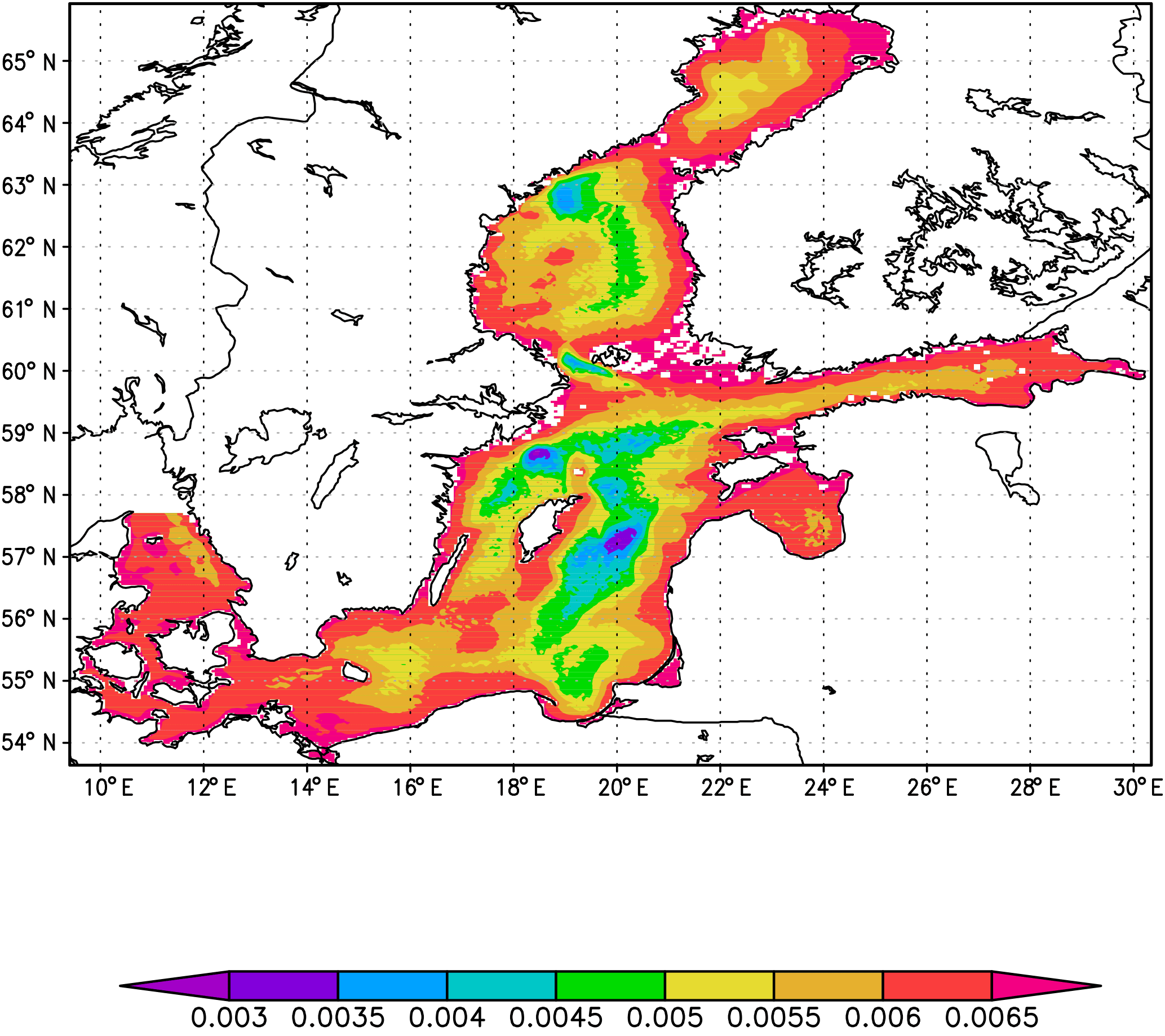
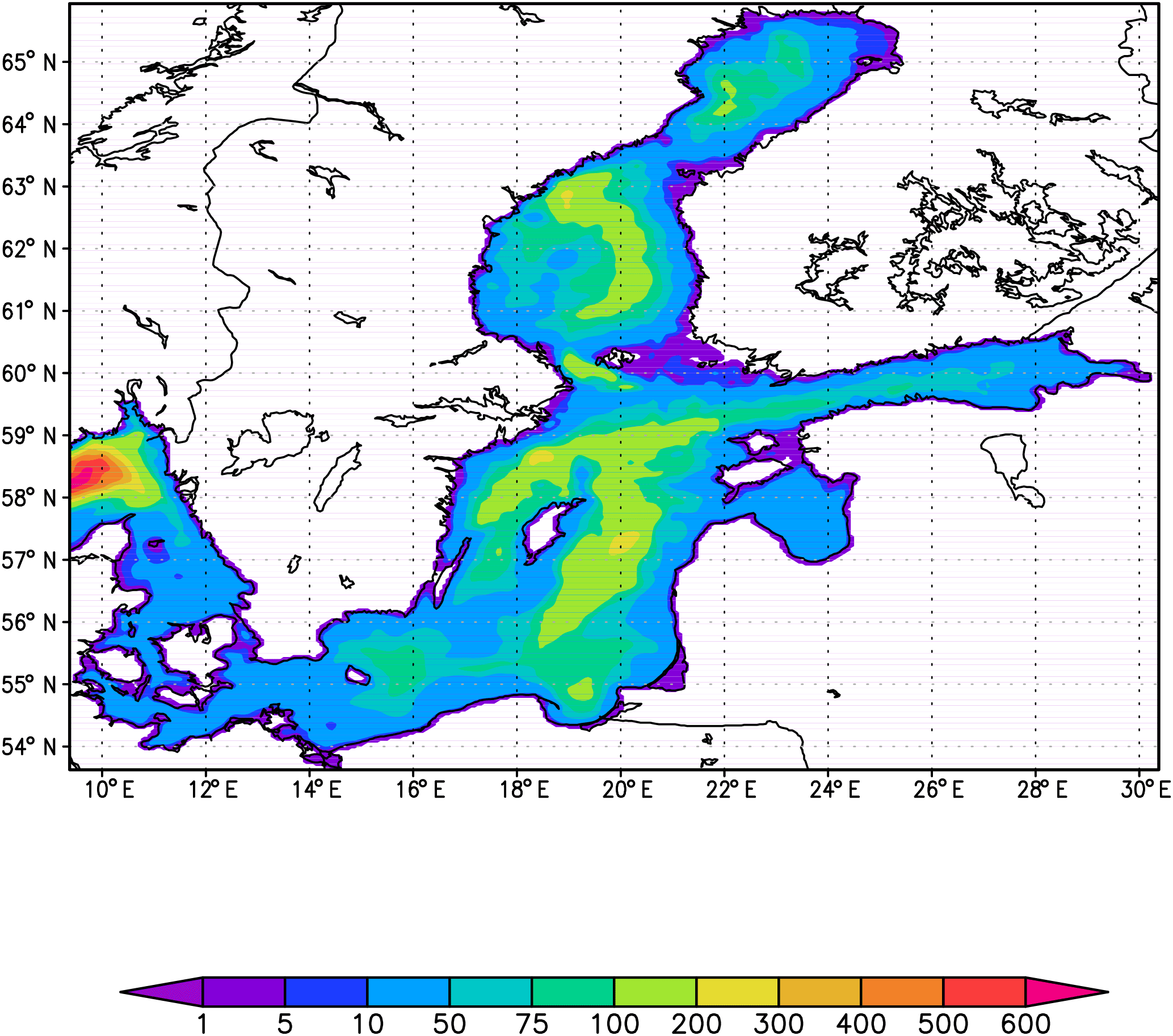
We can see the sub-areas (in red) in which the functional G(T) is most sensitive to errors in the observations during assimilation. The largest values of the gradient of G(T) correspond to the points x,y lying near the regions with a small depth (cf. sea topography, Fig. 2). One explanation of this phenomenon may be the fact that in the areas with depths of about 50 m, rapid convection occurs in the upper mixed layer. With the assimilation of the surface temperature, information is transmitted faster to shallower depths, which in turn contributes to a higher sensitivity to data in these places, in contrast to deeper regions.

Figure 2 Baltic Sea topography (m).

Remark 3. We use the discretize-then-optimize approach, and for numerical experiments all the presented equations are understood in a discrete form, as finite-dimensional analogues of the corresponding problems, obtained after approximation. This allows us to consider model equations as a perfect model, with no approximation errors. Therefore, the accuracy of the sensitivity estimates given by Eqs. (63)–(65) are determined by the accuracy of solving the Hessian equation ℋχ=Φ (step 2 of the algorithm). Due to Eqs. (56)– (58), this equation is equivalent to a linear data assimilation problem, and an approximate solution to the minimization problem is obtained by an iterative procedure.

The above studies allow us to solve the problem of the definition of sea sub-areas in which the functional of the optimal solution is most sensitive to errors in the observations during variational data assimilation, when the error values are not a priori known.

8 Conclusions

In this paper we have considered numerical algorithms to study the sensitivity of functionals of the optimal solution of the variational data assimilation problem aimed at the reconstruction of unknown parameters of the model. The optimal solution obtained as a result of assimilation depends on the observations that may contain uncertainties. Computing the gradient of the functionals with respect to observations reduces to the solution of a nonstandard problem which is a coupled system involving direct and adjoint equations with mutually dependent variables. Solvability of the nonstandard problem is related to the properties of the Hessian of the original cost function. An algorithm developed to compute the gradient of the response function is based on the second-order adjoint techniques. A numerical example for the variational data assimilation problem related to sea surface temperature for the Baltic Sea thermodynamics model demonstrates the result of the gradient computation of the response function associated with the mean surface temperature. The presented algorithm may be used to determine the sea sub-areas in which the functionals of the optimal solution are most sensitive to errors in the observations during variational data assimilation.