the Creative Commons Attribution 4.0 License.
the Creative Commons Attribution 4.0 License.
 | 02 May 2018
Idealized models of the joint probability distribution of wind speeds
Adam H. Monahan
The joint probability distribution of wind speeds at two separate locations in space or points in time completely characterizes the statistical dependence of these two quantities, providing more information than linear measures such as correlation. In this study, we consider two models of the joint distribution of wind speeds obtained from idealized models of the dependence structure of the horizontal wind velocity components. The bivariate Rice distribution follows from assuming that the wind components have Gaussian and isotropic fluctuations. The bivariate Weibull distribution arises from power law transformations of wind speeds corresponding to vector components with Gaussian, isotropic, mean-zero variability. Maximum likelihood estimates of these distributions are compared using wind speed data from the mid-troposphere, from different altitudes at the Cabauw tower in the Netherlands, and from scatterometer observations over the sea surface. While the bivariate Rice distribution is more flexible and can represent a broader class of dependence structures, the bivariate Weibull distribution is mathematically simpler and may be more convenient in many applications. The complexity of the mathematical expressions obtained for the joint distributions suggests that the development of explicit functional forms for multivariate speed distributions from distributions of the components will not be practical for more complicated dependence structure or more than two speed variables.
- Article
(1827 KB) - Full-text XML
- BibTeX
- EndNote


A fundamental issue in the characterization of atmospheric variability is that of dependence: how the state of one atmospheric variable is related to that of another at a different position in space, or point in time. The simplest measure of statistical dependence, the correlation coefficient, is a natural measure for Gaussian-distributed quantities but does not fully characterize dependence for non-Gaussian variables. The most general representation of dependence between two or more quantities is their joint probability distribution. The joint probability distribution for a multivariate Gaussian is well known, and expressed in terms of the mean and covariance matrix (e.g. Wilks, 2005; von Storch and Zwiers, 1999). No such general expressions for non-Gaussian multivariate distributions exist. Copula theory (e.g. Schlözel and Friederichs, 2008) allows joint distributions to be constructed from specified marginal distributions. However, which copula model to use for a given analysis is not generally known a priori and is usually determined empirically through a statistical model selection exercise.
The present study considers the bivariate joint probability distribution of wind speeds. As these are quantities which are by definition bounded below by zero, the joint distribution and the marginal distributions are non-Gaussian. While the correlation structure (equivalently, the power spectrum) of wind speeds in time (e.g. Brown et al., 1984; Schlax et al., 2001; Gille, 2005; Monahan, 2012b) and in space (e.g. Carlin and Haslett, 1982; Nastrom and Gage, 1985; Wylie et al., 1985; Brown and Swail, 1988; Xu et al., 2011) has been considered, relatively little attention has been paid to developing expressions for the joint distribution. Previous studies have used copula methods to model horizontal spatial dependence of wind speeds for wind power applications (Grothe and Schnieders, 2011; Louie, 2012; Veeramachaneni et al., 2015) and dependence of daily wind speed maxima (Schlözel and Friederichs, 2008). While these earlier analyses have focused on probabilistic modelling of simultaneous wind speed values at different spatial locations in the horizontal, dependence structures in the vertical (e.g. for vertical interpolation of wind speeds) or in time are also of interest. For example, an analysis in which the need for an explicit parametric form for the joint distribution of wind speeds at different altitudes has arisen is the hidden Markov model (HMM) analysis considered in Monahan et al. (2015). In an HMM analysis of continuous variables, it is necessary to specify the parametric form of the joint distribution within each hidden state. In Monahan et al. (2015), the joint distribution of wind speeds at 10 and 200 m and the potential temperature difference between these altitudes was modelled as a multivariate Gaussian distribution, despite the fact that for at least the speeds this distribution cannot be strictly correct. This pragmatic modelling approximation was made because of the absence of a more appropriate parametric distribution for the quantities being considered. The alternative approach of using the wind components at the two levels (for which the multivariate Gaussian model may be a better approximation) instead of the speeds directly has the downside of increasing the dimensionality of the state vector from three to five, dramatically increasing the number of parameters to be estimated (with the covariance matrices in particular increasing from 9 to 25 elements) and reducing the statistical robustness of the results.
A number of previous studies have constructed univariate speed distributions starting from models for the joint distribution of the horizontal components (e.g. Cakmur et al., 2004; Monahan, 2007; Drobinski et al., 2015). One useful benefit of this approach is that it allows the statistics of the speed and the components to be related to each other. The specific goal of the present study is to extend this approach to bivariate distributions, constructing models of the joint probability distribution of wind speeds that are directly connected to the joint distributions of the horizontal components of the wind. As the following results will demonstrate, generalizing this approach to the bivariate speed distribution results in rather complicated mathematical expressions. Expressions for multivariate distributions of more than two speeds will be even more complicated, and may not be analytically tractable. Through the analysis of the bivariate speed distribution, we will probe how far the development of closed-form, analytic expressions for parametric speed distributions based on distributions of components can practically be extended.
Both Weibull and Rice distributions have been used to model the univariate wind speed distribution (cf. Carta et al., 2009; Monahan, 2014; Drobinski et al., 2015), and models of multivariate distributions with Weibull or Ricean marginals have been developed (e.g. Crowder, 1989; Lu and Bhattacharyya, 1990; Kotz et al., 2000; Sagias and Karagiannidis, 2005; Yacoub et al., 2005; Mendes and Yacoub, 2007; Villanueva et al., 2013). Much of this work has been done in the context of wireless communications (Sagias and Karagiannidis, 2005; Yacoub et al., 2005; Mendes and Yacoub, 2007): the present study builds upon the results of these earlier analyses.
The two probability density functions (pdfs) we will consider, the bivariate Rice and Weibull distributions, both start with simple assumptions regarding the distributions of the wind components. The bivariate Rice distribution follows directly from the assumption of Gaussian components with isotropic variance, but nonzero mean. In contrast, the bivariate Weibull distribution is obtained from nonlinear transformations of the magnitudes of Gaussian, isotropic, mean-zero components. While the univariate Weibull distribution has been found to generally be a better fit to observed wind speeds than the univariate Rice distribution (particularly over the oceans, e.g. Monahan, 2006, 2007), the direct connection of the Rice distribution to the distribution of the components (which the Weibull distribution does not have) is useful from a modelling and theoretical perspective (e.g. Cakmur et al., 2004; Monahan, 2012a; Culver and Monahan, 2013; Sun and Monahan, 2013; Drobinski et al., 2015). The six-parameter bivariate Rice distribution that we will consider is more flexible than the five-parameter bivariate Weibull distribution, and able to model a broader range of dependence structures. Furthermore, it is directly connected to the univariate distributions and dependence structure of the wind components. However, the bivariate Weibull distribution is mathematically much simpler than the bivariate Rice distribution and easier to use in practice. Other flexible bivariate distributions for non-negative random variables exist, such as the α-μ distribution discussed in Yacoub (2007). Because the Weibull and Rice distributions are common models for the univariate wind speed distributions, this study will focus specifically on their bivariate generalizations.
The bivariate Rice and Weibull distributions are developed in Sect. 2, starting from discussion of the bivariate Rayleigh distribution (which is a limiting case of both of the other models). In this section, we repeat some of the formulae obtained by Sagias and Karagiannidis (2005), Yacoub et al. (2005), and Mendes and Yacoub (2007) for completeness and because of notational differences between this study and the earlier ones. In Sect. 3, the ability of these distributions to model wind speed data from the middle troposphere, and from the near-surface flow over land and the ocean, is considered. Examples of dependence structures in both space (horizontally and vertically) and in time are considered. A discussion and conclusions are presented in Sect. 4.
As a starting point for developing models of the bivariate wind speed distribution, we consider the joint distribution of the horizontal wind vector components , i=1, 2 (where the subscripts i denote wind vectors at two different locations, two different points in time, or both). In particular, we assume that
-
the two orthogonal wind components are marginally Gaussian with isotropic and uncorrelated fluctuations:
-
and the cross-correlation matrix of the two vectors is
where we have expressed the correlations in both Cartesian and polar coordinates: , with . This assumed correlation structure implies that the correlation matrix becomes diagonal when the vector u2 is rotated through the angle −ψ:
where
The joint distribution of the horizontal components resulting from these assumptions is
Note that only considering the horizontal components of the wind vector implicitly restricts the resulting distributions to timescales sufficiently long that the vertical component of the wind contributes negligibly to the speed.
2.1 Bivariate Rayleigh distribution
The joint distributions of the speeds obtained from the pdf Eq. (5) when both vector wind components are mean-zero is the bivariate Rayleigh distribution (e.g. Battjes, 1969). Transforming variables to wind speed wi and direction , the joint distribution (Eq. 5) with , , becomes
Integrating over the wind directions to obtain the marginal distribution for the wind speeds, we obtain
where we have used the fact that
where Ik(z) is the modified Bessel function of order k. Note that the correlation angle ψ drops out after integration over θ1 and θ2. As a result, for the bivariate Rayleigh distribution, p(w1,w2) depends only on the three parameters .
For ρ=0, p(w1,w2) factors as the product of the marginal distributions of w1 and w2:
and the wind speeds are independent. As ρ→1, we can use the asymptotic result
to show that
where δ(⋅) is the Dirac delta function. In this limit, w1 and w2 are perfectly correlated and Rayleigh distributed.
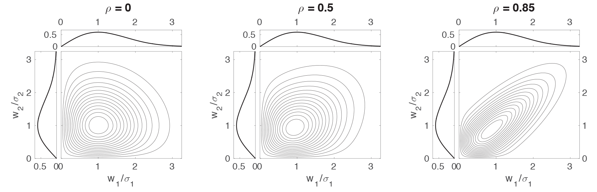
Figure 1Example bivariate Rayleigh distributions p(w1,w2) for , and 0.85, with w1 and w2 scaled respectively by σ1 and σ2. The upper and left subpanels show the marginal distributions of w1 and w2 respectively. These marginal distributions are the same for all three panels.
Moments of the bivariate Rayleigh distribution are given by
where is the hypergeometric function (Gradshteyn and Ryzhik, 2000). In particular, we have
Because is an increasing function of ρ2 with , corr(w1,w2) must be non-negative for the bivariate Rayleigh distribution.
Plots of p(w1,w2) for the three values ρ=0, 0.5, and 0.85 are presented in Fig. 1, along with the marginal distributions of w1 and w2 (which are the same for all three panels). The marginal distributions are positively skewed and the contours of the joint distributions are more tightly concentrated below and to the left of their peaks than elsewhere. As expected, the distributions become more tightly concentrated around the 1 : 1 line as the dependence parameter ρ increases.
2.2 Bivariate Rice distribution
The assumptions leading to the bivariate Rayleigh distribution are too restrictive to model observed wind speeds in most circumstances. A more general distribution results from assuming that the wind components are Gaussian, isotropic, and uncorrelated, but with nonzero mean (Eq. 5).
Changing variables to wind speed wi and direction θi, the joint distribution becomes
where
and where we have defined the magnitude and direction of the mean vector wind:
The marginal distribution for the wind speeds is obtained by integrating the joint distribution over θ1 and θ2. To evaluate this integral, we make use of the result
where
and it is important that be evaluated as the angle between the vector (a,b) and the vector (1,0) (that is, as the four-quadrant inverse tangent). Equation (22) follows from the Fourier series
along with repeated use of trigonometric identities and the integral Eq. (8).
Finally, we obtain the expression for the bivariate Rice distribution (Mendes and Yacoub, 2007)
Expressed in terms of the magnitude and direction of the mean wind vectors,
where
and
When numerically evaluating the bivariate Rice distribution, it is convenient to transform the infinite series in Eqs. (25) and (26) into an integral which is then approximated numerically (Appendix A).
Note that p(w1,w2) depends on the relative orientation of the mean wind vectors and the correlation angle ψ only through the combination . Because of this symmetry, the quantities ϕ1−ϕ2 and ψ cannot be determined individually from wind speed data alone. As a result, p(w1,w2) is determined by six parameters: ). For particular applications, it may be appropriate to fix either ϕ1−ϕ2 or ψ, allowing the other angle to be estimated from data. For example, when considering the temporal dependence structure of winds assumed to have stationary statistics, it can be assumed that . The bivariate Rice distribution also has the discrete symmetry that it is invariant under the transformation . Note that these symmetries are in addition to the invariance of the distribution of components (Eq. 5) to the rotation of the coordinate system , , under which the angles ϕ1−ϕ2 and ψ are individually invariant.
Integrating over w2 to obtain the marginal distribution for w1 we obtain the univariate Rice distribution
with mean and variance
(with equivalent expressions for w2 obtained by integrating over w1), where is the confluent hypergeometric function (Gradshteyn and Ryzhik, 2000). Equation (29) follows from Eq. (25) using the integral (Gradshteyn and Ryzhik, 2000)
Neumann's theorem (Watson, 1922)
and the fact that
Note that each wind speed marginal distribution depends only on the magnitude of the mean wind vector, while the joint distribution also depends on the angle between the two mean wind vectors. Furthermore, as ρ→0 only the first term contributes to the infinite series in Eq. (25), and the joint distribution reduces to the product of the marginals.
The joint moments of the bivariate Rice distribution can be evaluated using the Taylor series expansion:
which allows the double integral defining the moments to factorize as the products of individual integrals over w1 and w2 that can be evaluated using
The resulting expression for the joint moments is
(Mendes and Yacoub, 2007). When the mean vector winds are equal to zero, only the k=0 terms contribute to this expression and Eq. (12) is recovered.

Defining the variables , the correlation coefficient between w1 and w2 is given by
where
The correlation coefficient corr(w1,w2) depends only on the four quantities . Monahan (2012b) considered the correlation structure of wind speeds using the approximation . The assumed covariance structure of the wind components then results in the approximate expression:
Plots of the correlation coefficient (Eq. 38) and the approximation (Eq. 40) as functions of ρ are shown in Fig. 2 for = (3,2,0) and (1,5,0). Agreement between the exact and approximate values of the correlation coefficient is reasonably good in both cases, with the largest discrepancies generally occurring for larger absolute values of ρ. Note that negative wind speed correlation values are permitted by the bivariate Rice distribution.
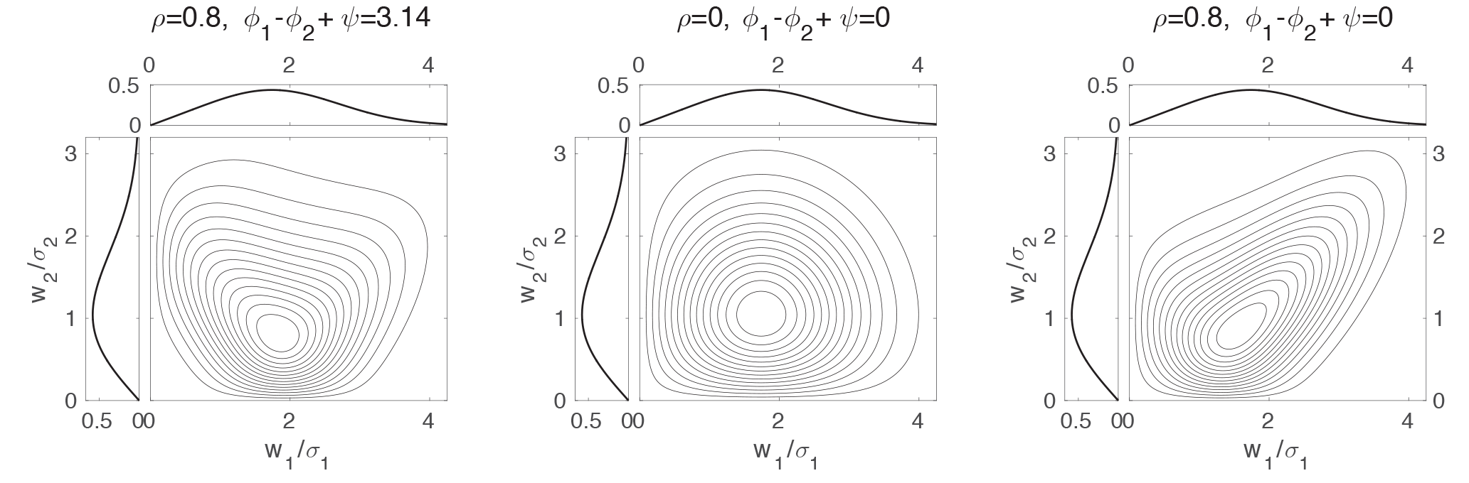
Examples of the joint Rice pdf (and the associated marginals) are presented in Fig. 3 for and , and (0.85,0). By construction, the marginal distributions are the same in each panel. The distributions of both w1 and w2 are positively skewed, and take respective maxima at values of about σ1 and just less than 2σ2. For the different values of the dependence parameter ρ, the joint distributions have considerably different shapes. The joint distribution for describes (weakly) negatively correlated variables with a nonlinear dependence structure evident in ridges of enhanced probability extending to the left and right upward from the probability maximum. For , probability contours are concentrated towards smaller values of w1 and w2 (as is the case for the marginal distributions). Finally, w1 and w2 are evidently positively correlated for , with a slight curvature in the shape of the distribution indicating the existence of some nonlinear dependence.
Although the bivariate Rice distribution differs from the bivariate Rayleigh distribution only by allowing for nonzero mean wind vector components, the resulting expressions for the joint pdf (Eq. 25) and the moments (Eq. 37) are much more complicated for the bivariate Rice than the bivariate Rayleigh. Furthermore, while the univariate Rice distribution is a convenient model for the pdf of wind speed, observed winds show clear deviation from Ricean behaviour (e.g. Monahan, 2006, 2007). We will therefore consider another model of the bivariate wind speed distribution with Weibull marginals, which turns out to result in simpler mathematical expressions (at the cost of a more artificial derivation than that of the bivariate Rice distribution).
2.3 Bivariate Weibull distribution
As in Sagias and Karagiannidis (2005) and Yacoub et al. (2005), we obtain the bivariate Weibull distribution from the bivariate Rayleigh distribution through separate power law transformations of w1 and w2. The pdf of a Weibull distributed variable is
with moments
where a and b are denoted the scale and shape parameters respectively. The Rayleigh distribution is a special case of the Weibull distribution with and b=2. Weibull distributed variables remain Weibull under a power law transformation, with suitably modified scale and shape parameters: if x is Weibull with scale parameter a and shape parameter b, xk will be Weibull with scale parameter ak and shape parameter b∕k. A joint wind speed distribution with Weibull marginal distributions can therefore be constructed from a joint Rayleigh distribution using the appropriate power law and scale transformations.
If we start with (x1,x2) as bivariate Rayleigh distributed with , , we obtain marginal Weibull distributions with specified scale and shape parameters through the transformations
The joint pdfs transform as
and so we obtain the bivariate Weibull distribution
An analogous approach to constructing bivariate Weibull distributions through nonlinear transformations of a bivariate Gaussian was followed in Villanueva et al. (2013); the resulting expressions are considerably more complicated than those considered here.
Evidently, p(w1,w2) factorizes into the product of the marginal distributions as ρ→0. As ρ→1, we can use Eq. (10) to make the approximation
where the last equality follows from the fact that
As expected, w1 and w2 are completely dependent in the limit that ρ→1 (although they are not perfectly correlated if b1≠b2 as the functional relationship
between the two variables will be nonlinear).
The relatively simple form of the bivariate Weibull distribution permits a relatively simple expression for the conditional distribution
The factor in the second set of braces characterizes how conditioning on the value of w1 changes the distribution of w2 from its marginal distribution (and corresponds to a copula density; e.g. Schlözel and Friederichs, 2008). Note that for w1 sufficiently large we can write
For ρ not too close to zero, the conditional distribution for large w1 is concentrated around the nonlinear regression curve
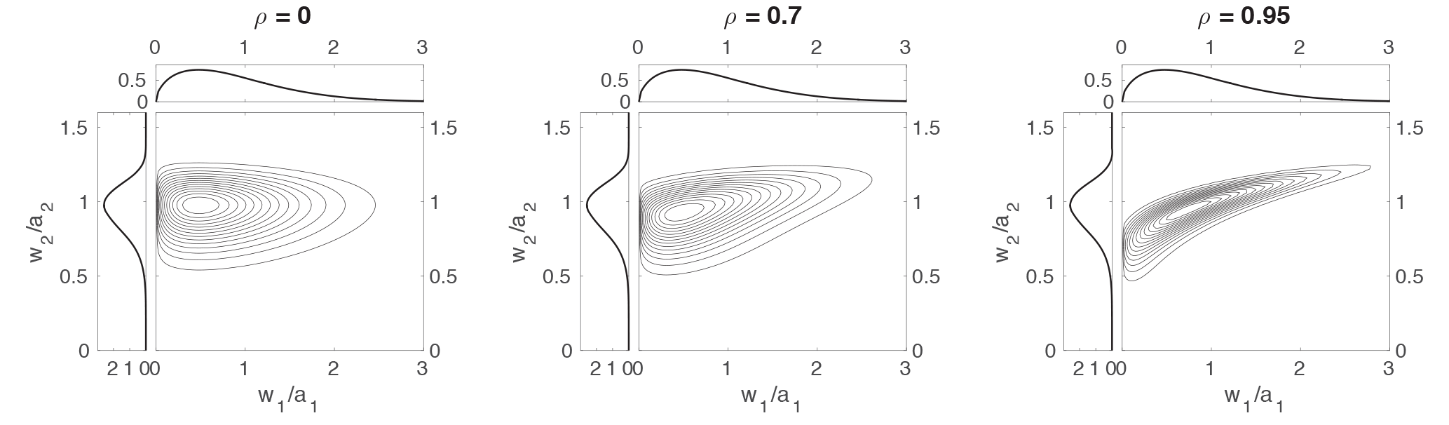
Figure 4As in Fig. 1 for the bivariate Weibull distribution with and , and 0.95 and the speeds w1,w2 scaled respectively by the Weibull scale parameters a1, a2.
Computing the moments, we obtain
(Sagias and Karagiannidis, 2005; Yacoub et al., 2005). The correlation coefficient is then given by
For (the relevant range of shape parameters for wind speeds), is an increasing function of ρ2 with . Therefore, the bivariate Weibull distribution is unable to represent situations in which the wind speeds are negatively correlated.
Examples of the bivariate Weibull distribution for and values of , and 0.95 are shown in Fig. 4. Again, the marginal distributions in all three cases are the same by construction. The distribution of w1 is positively skewed with a maximum near a value of w1=0.5a1, while that of w2 is negatively skewed with a maximum near w2=a2. For ρ=0 the joint distribution is simply the product of the marginals. As ρ increases, w1 and w2 become positively correlated - although the correlation is weak even for ρ=0.7 for this set of parameter values. At the value of ρ=0.95, while the correlation of the two variables is only moderate, a strong nonlinear dependence is evident in the concentration of the distribution around the curve given by Eq. (48).
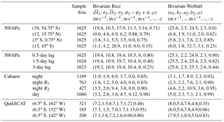
Many wind datasets from different locations are available, and it is impracticable to consider joint distributions of wind speeds from even a small fraction of these. In this section, we will consider examples of the joint distribution of wind speeds using data from a representative range of settings. Bivariate distributions of wind speeds at both different locations in space and different points in time will be considered. The sampling of the wind speeds considered will be temporal (that is, individual samples will correspond to a specific time for spatial joint pdfs and a specific pair of times for temporal joint pdfs). Best-fit values of the parameters of the bivariate Weibull and Rice distributions we present were obtained numerically as maximum likelihood estimates (Table 1), with ϕ1−ϕ2 set to zero. Goodness-of-fit of the distributions was assessed using a statistical test described in Appendix B. In order to distinguish how well the parametric joint distributions model the marginal distributions from how well they represent dependence between variables, the goodness-of-fit analyses were repeated for each pair of time series with the values of one of the pair shuffled in time. This shuffling destroys the dependence structure without affecting the distributions of the marginals. Use of a bivariate analysis rather than separate univariate goodness-of-fit tests for the marginals allows direct comparisons of p-values, as exactly the same test is used for the original and shuffled data.
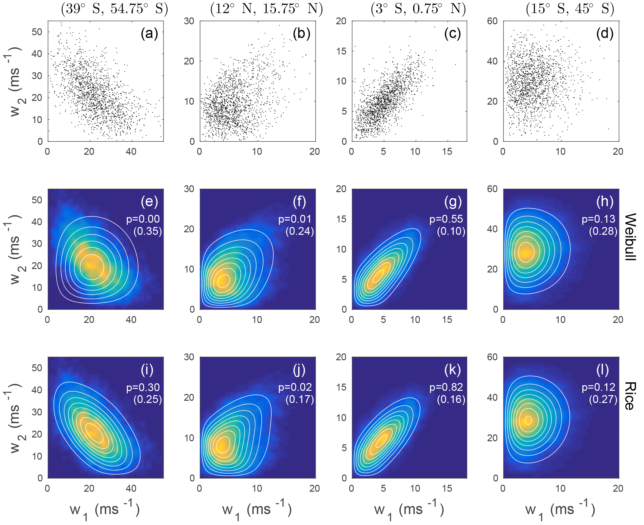
Figure 5Joint distributions of 500 hPa DJF 00Z wind speeds at four different pairs of latitudes along 216∘ W. Wind speeds at the two latitudes quoted in the column headings are respectively denoted w1 and w2. (a–d) Scatterplots of wind speed data. (e–h) Maximum likelihood bivariate Weibull pdfs (white contours) and kernel density estimates of the observed joint pdf (colours). The p-value of a goodness-of-fit test with the null hypothesis that the observed wind speed data are drawn from the corresponding best-fit bivariate Weibull distribution is given. The values in brackets are the p-values obtained when the dependence structure is eliminated by shuffling the values of w2 in time. (i–l) As in the middle row, for the best-fit bivariate Rice distribution. Values of the best-fit model parameters are given in Table 1.
3.1 Wind speeds at 500 hPa
We first consider the joint distribution of 00Z December, January, and February 500 hPa wind speeds from 1979 to 2014. These data were taken from the European Centre for Medium-Range Weather Forecasts (ECMWF) ERA-Interim Reanalysis (Dee et al., 2011), subsampled to every second day to minimize the effect of serial dependence on the goodness-of-fit test (Monahan, 2012b). The wind speed data were computed as the magnitude of zonal and meridional components.
The joint distributions of wind speeds at four pairs of latitudes along 216∘ W are presented in Fig. 5. A moderately strong negative correlation () is evident between wind speeds at (39∘ S, 216∘ W) and (54.75∘ S, 216∘ W) (Fig. 5a). Because it is unable to model a negative correlation between wind speeds, the best-fit bivariate Weibull pdf differs substantially from the distribution of the observed winds (Fig. 5e). The goodness-of-fit test correspondingly rejects the null hypothesis that the observations are drawn from this distribution (p=0). In contrast, the bivariate Rice distribution provides a reasonable model of the joint distribution of wind speeds at these two locations (Fig. 5i) and the goodness-of-fit test provides no evidence that these data are statistically incompatible with this distribution (p=0.31). For wind speeds at these two locations, the bivariate Rice distribution is evidently a better model than the bivariate Weibull distribution.
In contrast, for wind speeds at (12∘ N, 216∘ W) and (15.75∘ N, 216∘ W), the null hypotheses of being drawn from either the bivariate Rice or Weibull distributions are rejected at the 95 % significance level for both distributions. These wind speeds are weakly correlated (r=0.37) but show evidence of nonlinear dependence. The joint pdf of the observed speeds is characterized by two ridges of high probability extending to the right, upward and downward away from the region of maximum probability (Fig. 5b, f, j). These ridges are not captured by either of the best-fit bivariate Weibull or Rice distributions, although a hint of this structure is evident in the Rice distribution. While the fit of one or both of these parametric distributions to these observed wind speed data may be sufficiently good for practical applications, nevertheless we can confidently exclude the possibility that these data are drawn from either distribution.
The wind speeds at (3∘ S, 216∘ W) and (0.75∘ N, 216∘ W) are correlated (r=0.68) and their scatter clusters around a straight line extending away from the origin (Fig. 5c). Both the best-fit bivariate Weibull and Rice distributions appear to the eye to be good fits to the data (Fig. 5g, k), and in neither case can the null hypothesis be rejected that the data are drawn from these distributions. Only small differences exist between the two best-fit distributions for these data.
Finally, the wind speeds at (15∘ S, 216∘ W) and (45∘ S, 216∘ W) are uncorrelated (r=0.06) and fit sufficiently well by both the bivariate Weibull and Rice distributions (Fig. 5d, h, l) that in neither case is the null hypothesis rejected. As in the previous example, the bivariate best-fit Rice and Weibull distributions are essentially indistinguishable for these data.
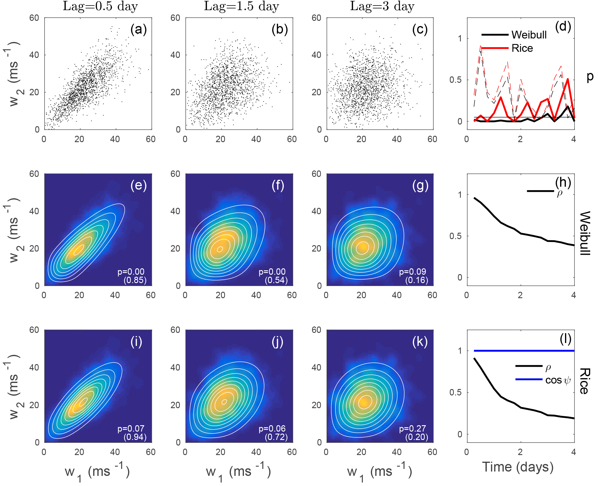
Figure 6The temporal dependence structure of 500 hPa DJF 00Z wind speeds at (39∘ S, 216∘ W) for lags s = 0.25 to 4 days, with w1=w(tn) and . (a–c) Scatterplots of wind speeds separated by 0.5 days (first column), 1.5 days (second column), and 3 days (third column). (e–g) Maximum likelihood bivariate Weibull distribution (white contours) and kernel density estimate of the joint pdf of the lagged data. The p-value of a goodness-of-fit test of the bivariate Weibull fit is quoted in white. The values in brackets are the p-values obtained when the dependence structure is eliminated by shuffling the values of w2 in time. (i–k) As in panels (e–g) for the bivariate Rice distribution. Panels (d, h, l) show results at a range of different time lags. (d) p-values of bivariate goodness-of-fit tests for bivariate Weibull (solid black) and bivariate Rice (solid red). The dashed lines correspond to the p-values for shuffled w2. The thin black curve is the 0.95 significance level. (h) Best-fit estimate of the parameter ρ of the bivariate Weibull distribution. (l) Best-fit estimates of ρ (black) and cos ϕ (blue) for the Rice distribution. Values of the best-fit model parameters are given in Table 1.
Considering the spatial correlation structure of these 500 hPa winds, we find cases in which one distribution (the Rice) is evidently a better fit to the data than the other (the Weibull), in which neither distribution provides a statistically significant fit to the data, and in which both distributions fit the data equally well. p-values from the analyses with temporally shuffled data, quoted in parentheses in Fig. 5, show that for none of the four pairs of wind speeds considered can the null hypotheses of univariate Weibull or univariate Rice distributions for the pair of marginals be rejected. This result indicates that for these data the rejection of the full bivariate distributions occurs because of a failure to adequately represent the dependence structure between the two random variables.
The temporal dependence structure of the wind speed at (39∘ S, 216∘ W) is illustrated in Fig. 6. As with the previous calculations, the pairs of lagged wind speeds were subsampled to 2-day resolution to minimize the effect of serial dependence on the results of the goodness-of-fit tests. As the lag increases, the value of the dependence parameter ρ decreases as expected for both the Weibull and Rice distributions (Fig. 6h, l). For most lags, the null hypothesis of the Weibull distribution as a model for the joint distribution is rejected (p<0.05; Fig. 6d). The rejection of the null hypothesis of a bivariate Weibull distribution is most robust for lags shorter than 3 days. In contrast, the null hypothesis of a bivariate Rice distribution is rejected less often than it is not – although p<0.05 for more than one-third of the lags (Fig. 6d). Inspection of the example distributions shown demonstrates that the bivariate Weibull distributions are broader around their principal axis for small to intermediate wind speeds in a way that is not consistent with observations (Fig. 6e–g). Such structures are not seen in the best-fit Rice distributions (Fig. 6i–k). Note that for lags of 0.5 and 1.5 days the observed distributions suggest a flaring out of the joint distribution for large wind speeds that is accounted for by neither the bivariate Weibull nor Rice distributions. There is good evidence that these data were not drawn from a bivariate Weibull distribution, and the evidence that they are drawn from a bivariate Rice distribution is not strong. p-values of fits obtained after shuffling of the lagged wind speed time series (in brackets in Fig. 6e–g, i–k and dashed lines in Fig. 6d) are generally larger than those of the unshuffled data: with a few exceptions (e.g. a lag of 1.75 days), the rejection of the null hypothesis of the full dataset being drawn from either of the parametric distributions considered is not associated with a failure to fit the marginals.
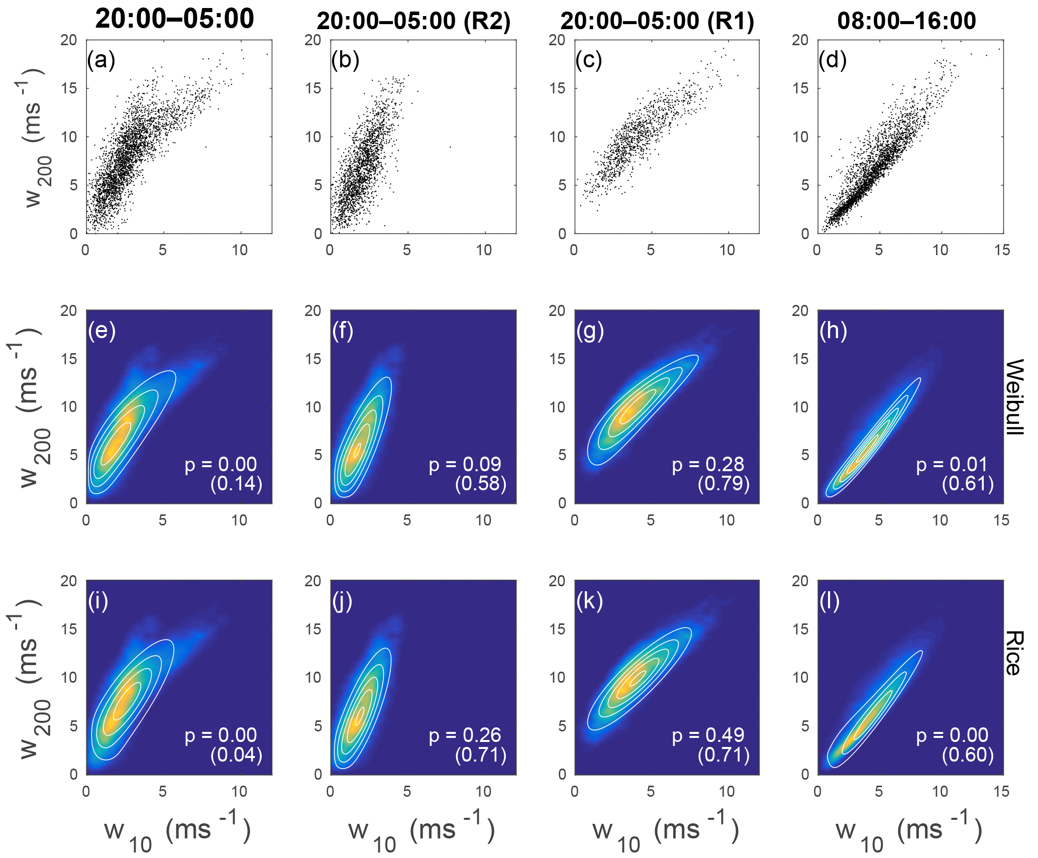
Figure 7Joint distribution of JAS wind speeds at 10 and 200 m measured at Cabauw, NL. (a–d) Wind speed scatterplots. (e–h) Kernel density estimate of the joint pdf of wind speeds (colour) and maximum likelihood bivariate Weibull distribution (contours). The p-value of a goodness-of-fit test of the bivariate Weibull distribution is quoted in white. The values in brackets are the p-values obtained when the dependence structure is eliminated by shuffling the values of w200 in time. (i–l) As in the middle row, but for the best-fit bivariate Rice distribution (contours). (a, e, i) All nighttime data (20:00–05:00 UTC). (b, f, j) Nighttime data conditioned on being in regime R2 (very stable boundary layer). (c, g, k) Nighttime data conditioned on being in regime R1 (weakly stable boundary layer). (d, h, l) All daytime data (08:00–16:00 UTC). Values of the best-fit model parameters are given in Table 1.
3.2 Wind speeds over land at 10 m and 200 m
We next consider wind speeds at altitudes of 10 and 200 m measured from a 213 m tower in Cabauw, Netherlands (51.971∘ N, 4.927∘ E), maintained by the Cabauw Experimental Site for Atmospheric Research (CESAR; van Ulden and Wieringa, 1996) with 10 min resolution from 1 January 2001 through 31 December 2012. We will focus on data from July, August, and September (JAS), separated into daytime (08:00–16:00 UTC) and nighttime (20:00–05:00 UTC) periods. These data were subsampled in time to account for serial dependence. Only every 50th point was used in the following analysis. A small number of zero wind speed values were removed from the dataset.
Monahan et al. (2011, 2015) demonstrated the existence of two distinct regimes of the nocturnal boundary layer in these data, corresponding to the very and weakly stratified boundary layers (vSBL and wSBL; e.g. Mahrt, 2014). These regimes, denoted respectively R1 and R2, were separated in Monahan et al. (2015) using a two-state HMM. Conditioning the data on the HMM state, the scatterplot of wind speeds at 10 and 200 m separates into two distinct populations (Fig. 7a–c). The scatter of wind speeds at these two altitudes shows no evident regime structure during the day (Fig. 7d). In all cases, the wind speeds at the two altitudes are highly correlated.
Maximum likelihood estimates of the bivariate Weibull and Rice distributions for the full nighttime data show evident disagreement between the scatter of the data and the best-fit distributions (Fig. 7e, i). Goodness-of-fit tests for both distributions were rejected (with p=0 in both cases). When conditioned on being in either regime R1 or R2, both the bivariate Rice and Weibull distributions result in much better representations of the nighttime data (Fig. 7f, g, j, k). In all cases the p-values exceed 0.05, so the fits cannot be rejected at the 95 % significance level. While neither the bivariate Rice nor Weibull distributions is a good probability model for the full joint distribution of wind speeds at these two altitudes, both are reasonable models for the distributions conditioned by regime occupation. Finally, the fits of neither the bivariate Rice nor Weibull distributions to the daytime data are statistically significant at the 95 % significance level. In particular, the joint Rice distribution is too broad (relative to observations) for small values of w10 and w200 and neither distribution is broad enough at higher wind speed values. p-values of fits with w200 shuffled in time are all larger than those of fits to the original data; only for the Rice fit to the full nighttime data is the shuffled p-value below 0.05. As seen in the previous data considered, there is no systematic evidence that the failure of the joint Weibull or Rice distributions to model the joint distributions of the Cabauw data results from a failure to model the marginals.
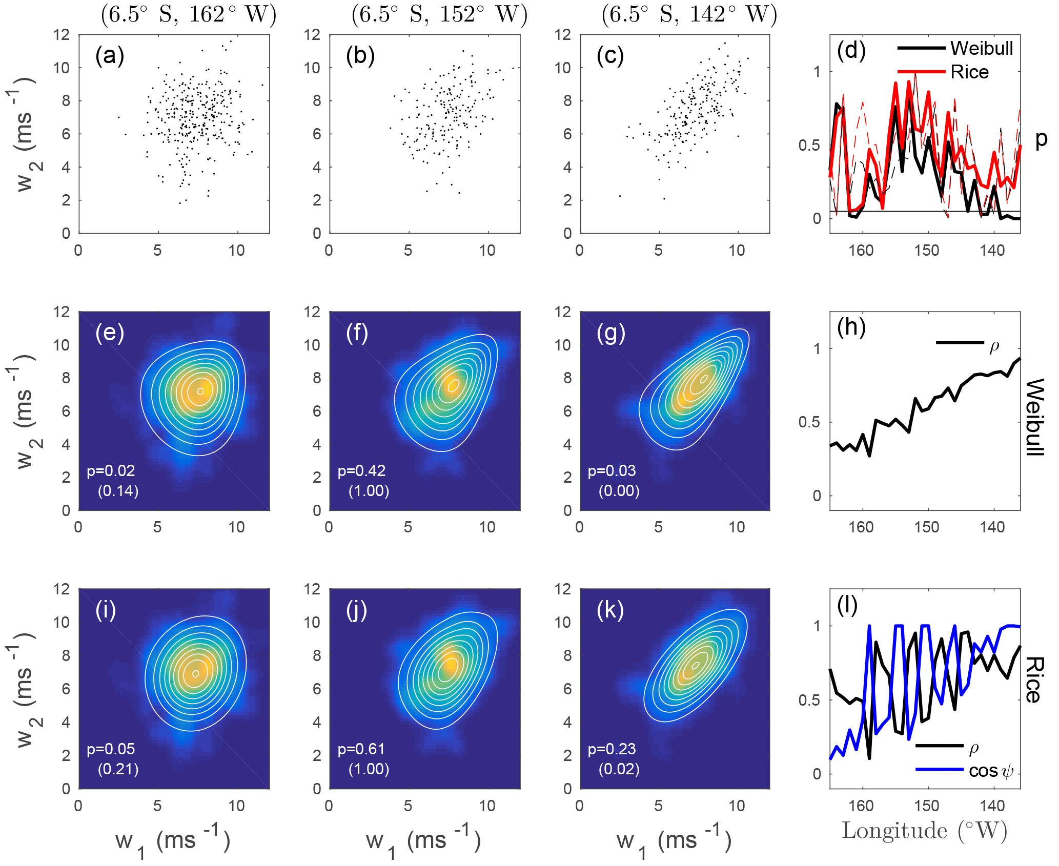
Figure 8Joint distribution of DJF QuikSCAT wind speeds at (6.5∘ S, 135∘ W), denoted w1, and westward along a zonal transect to 165∘ W (denoted w2). (a–c) Scatterplots of wind speed at (6.5∘ S, 135∘ W) and at the points (6.5∘ S, 162∘ W), (6.5∘ S, 152∘ W), and (6.5∘ S, 142∘ W). (e–g) Kernel density estimate of the joint pdf (colour) as well as the maximum likelihood bivariate Weibull distribution (white contours). The p-value of a goodness-of-fit test of the bivariate Weibull distribution is quoted in white. The values in brackets are the p-values obtained when the dependence structure is eliminated by shuffling the values of w2 in time. (i–k) As in panels (e–g) but for the bivariate Rice distribution. (d) p-values of the bivariate goodness-of-fit tests for the wind speeds along the transect, for the bivariate Weibull distribution (solid black) and for the bivariate Rice distribution (solid red). The dashed lines correspond to the p-values for shuffled w2. (h) Estimate of the parameter ρ from the best-fit bivariate Weibull distribution along the transect. (l) Estimate of the parameters ρ (black) and cos ψ (blue) from the best-fit bivariate Rice distribution along the transect. Values of the best-fit model parameters are given in Table 1.
3.3 Sea surface wind speeds
Twice-daily December, January, and February level 3.0 gridded SeaWinds scatterometer equivalent neutral 10 m wind speeds between 60∘ S and 60∘ N at a resolution of 0.25∘ × 0.25∘ from the National Aeronautics and Space Administration (NASA) Quick Scatterometer (QuickSCAT; Perry, 2001) are available from December 1999 through February 2008. Data flagged as having possibly been corrupted by rain were excluded from the following analysis. Although the data are nominally twice-daily, it is often the case that data for either the ascending or descending pass of the satellite are missing. The maximum likelihood parameter estimates of bivariate wind speed distributions and goodness-of-fit tests were carried out using every third non-missing data point in order to minimize the effect of serial dependence. For the goodness-of-fit tests M=10 quantiles were used because of the relatively small sample sizes. Because of the near-polar orbit of the satellite results, observations of wind speed at different locations are not simultaneous. The joint distributions we consider therefore combine dependence in both space and time.
Joint distributions of wind speed at (6.5∘ S, 135∘ W) with speeds at points along a zonal transect to 165∘ W (in increments of 1∘) were estimated. As the distance between the two positions increases, there is a decreasing trend in the best-fit bivariate Weibull dependence parameter ρ (Fig. 8h) with some small fluctuations likely due to sampling variability. The same is not true for the best-fit bivariate Rice dependence parameter ρ, which fluctuates wildly (Fig. 8l). Large fluctuations also seen in the best-fit value of cos ψ are clearly correlated with those of ρ: where one parameter is anomalously large (relative to the spatial trend), the other is anomalously small. Of the 30 pairs of points considered, the null hypothesis of a bivariate Rice distribution is rejected (at the 95 % significance level) at only one (Fig. 8d). In contrast, p<0.05 for the bivariate Weibull distribution at several longitudes, particularly close to the base point at (6.5∘ S, 135∘ W). Inspection of the best-fit bivariate Weibull pdfs (Fig. 8e–g) shows that they are broader for smaller wind speeds than for larger values, a feature not evident in the best-fit bivariate Rice distributions (Fig. 8i–k) or the scatter of data (Fig. 8a–c). From these results, we find only equivocal evidence that the pairs of wind speed data along this zonal transect are drawn from a bivariate Weibull distribution and no strong evidence to reject the null hypothesis that they are drawn from a bivariate Rice distribution. Again, the p-values of fits to temporally shuffled wind speeds are generally similar to or larger than those of fits to the full distribution. The bivariate Rice distribution with the wind speed at 142∘ W (Fig. 8k) illustrates a rare example in which the parametric fit to the original data passed the goodness-of-fit test at the 5 % significance level while the fit to the shuffled data did not; it is evident from Fig. 8d that this situation is not common. The surface wind vector components in the tropics are known to be non-Gaussian (e.g. Monahan, 2007), so we have a priori reasons to believe the joint distribution should not be Ricean. The fact that the data do not generally allow for a rejection of the null hypothesis that the winds are bivariate Rice (for either the original or shuffled datasets) is likely a consequence of the relatively small sample size.
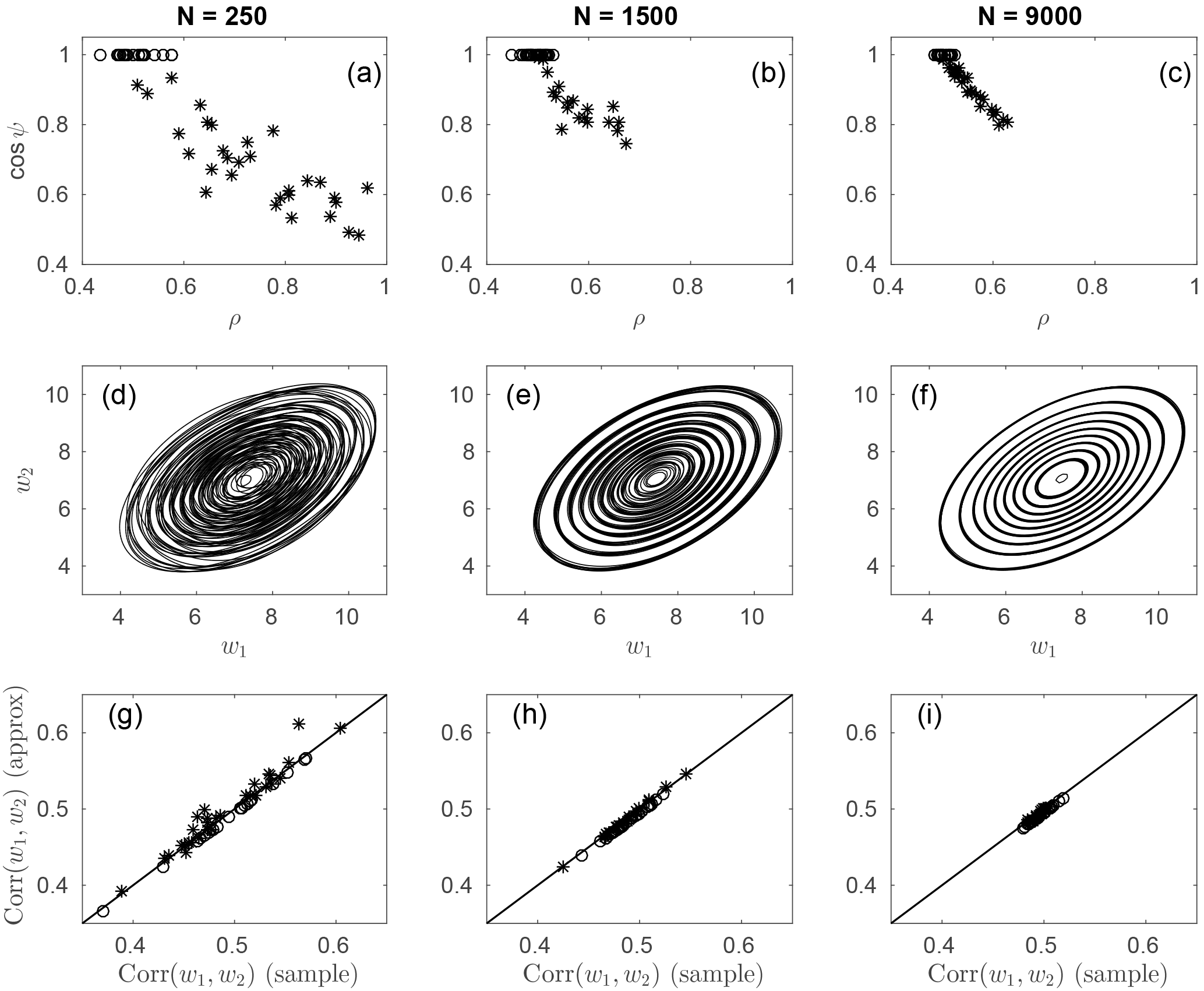
Figure 9(a–c) Estimates of ρ and cos ψ from 50 realizations of bivariate Ricean variables with for each of the sample sizes , and 9000. The open circles correspond to estimates with , while the stars are estimates with . (d–f) Contours of bivariate Rice pdfs corresponding to 10 of the 50 best-fit parameter estimates (randomly chosen). The contour values are the same for all pdfs within each subplot. (g–i) Scatterplot of the sample correlation coefficient between the two Ricean variables and the correlation coefficient given by the approximate expression Eq. (40). The 1 : 1 line is given in solid black. The open circles and stars are as in the upper row.
The large variations in best-fit estimates of ρ and cos ψ for the bivariate Rice distribution result from the fact that for some parameter values the distribution is only weakly sensitive to simultaneous changes in these parameters: increases in ρ can be offset by decreases in cos ψ with only small changes to the joint distribution. To demonstrate this weak sensitivity, 50 realizations of bivariate Ricean variables with were generated for each of the sample sizes of N=250, 1500, and 9000. Maximum likelihood estimates of these parameters obtained from these realizations demonstrate that for the smaller samples ρ and cos ψ show strong and correlated sampling variability, with large increases in ρ combined with large decreases in cos ψ (Fig. 9a). As expected, these sampling fluctuations become smaller as the sample size increases(Fig. 9b, c). Despite the large variation of ρ and cos ψ for small to intermediate sample sizes, there is relatively little variation in the structure of the corresponding bivariate Rice distributions (Fig. 9d–f).
An indication of why increases in ρ should counterbalance decreases in cos ψ with only small effects on the joint distribution is given by the approximate expression for the correlation coefficient, Eq. (40). The value of this approximation is unaffected by changes in ρ and ψ that leave the numerator invariant. The compensation between sampling variations in ρ and cos ψ is evident the fact that corr(w1,w2) given by Eq. (40) is an excellent approximation to the sample correlation coefficient even for estimates of ρ and cos ϕ which are far away from the population values (Fig. 9g–i). Note that there is no evident relationship between sampling fluctuations in corr(w1,w2) and those of ρ and ψ: the range of sample correlation values for (ρ,cos ψ) near the population values of (0.5,1) (open circles) is the same as that for values of (ρ,cos ψ) far from these values (stars). In these parameter ranges, the dependence between w1 and w2 constrains ρ and ψ not individually, but together – over large ranges of values for sufficiently small sample sizes.
This study has considered two idealized probability models for the joint distribution of wind speeds, both derived from models for the joint distribution of the horizontal wind components. The first, the bivariate Rice distribution, follows from assuming that the wind vector components are bivariate Gaussian with an idealized covariance structure. The second, the bivariate Weibull distribution, arises from nonlinear transformations of variables with a bivariate Rice distribution in the limit that the mean vector winds vanish (the bivariate Rayleigh distribution). While the bivariate Rice distribution has the advantage of being more flexible and naturally related to a simplified model for the joint distribution of the wind components, the bivariate Weibull distribution is mathematically much simpler and easier to work with. Through consideration of a range of joint distributions of observed wind speeds (over land and over the ocean; at the surface and aloft; in space and in time) the bivariate Rice distribution was shown to generally model the observations better than the bivariate Weibull distribution. However, in many circumstances the differences between the two distributions are small and the convenience of the bivariate Weibull distribution relative to the bivariate Rice distribution is a factor which may motivate its use.
The fact that the bivariate Rice distribution is easier to work with, but less flexible, than the bivariate Weibull distribution is evident from inspection of their analytic forms and the relative number of parameters to fit (five vs. six). If the bivariate Weibull distribution was generically appropriate for modelling the bivariate wind speed distribution, there would be no need to consider more complicated models such as the bivariate Rice. This study provides an empirical assessment of the relative practical utility of the two models, trading off the ability to model more general dependence structures (e.g. negatively correlated speeds) against model simplicity. Neither the univariate nor the bivariate Weibull or Rice distributions are expected to represent the true distributions of wind speeds (e.g. Carta et al., 2009). The results of this analysis characterize the practical utility of these models, rather than making a claim to their “truth”. It is noteworthy that for the data considered in this study, the failure of either the bivariate Rice or Weibull distributions to adequately fit the joint distribution of wind speeds (at a significance level of 5 %) is not generally associated with a corresponding failure of the parametric distribution to model the marginals. An interesting direction of future study would be consideration of other parametric models for the joint distribution of non-negative quantities, such as the α-μ distribution (Yacoub, 2007), copula-based models (e.g. Schlözel and Friederichs, 2008), or distributions obtained through nonlinear transformations of multivariate Gaussians (e.g. Brown et al., 1984).
Many of the assumptions that have been made regarding the distribution of the wind components are known not to hold in various settings. For example, the vector wind components are generally not Gaussian, either aloft or at the surface (e.g. Monahan, 2007; Luxford and Woollings, 2012; Perron and Sura, 2013), and fluctuations will not generally be isotropic (especially over land; cf. Mao and Monahan, 2017). Furthermore, when used to model temporal dependence the assumed correlation structure cannot account for the anisotropy in autocorrelation of orthogonal components in either space (e.g. Buell, 1960) or time (e.g. Monahan, 2012b). Relaxing the assumptions regarding isotropy of correlation structure results in expressions for the joint speed distributions involving integrals over angle which are not analytically tractable.
While it is possible to relax the assumption of Gaussian components for univariate speed distribution (e.g. Monahan, 2007; Drobinski et al., 2015), extending this analysis to the bivariate case would involve specifying a non-Gaussian dependence structure for the components. At present, there is no physically based model for such dependence. Without any such physical justification, the only option is an empirical investigation of the ability of different copula models to represent observed joint wind speed distributions. It is unlikely that a copula-based model for dependence of components will admit analytically tractable expressions for joint speed distributions. A copula-based analysis of either the components or the speeds directly is also likely necessary for modelling extreme wind speeds (either large percentiles, peaks over threshold, or block maxima), as the tails of the bivariate Rice and Weibull distributions may not be adequate for this task. Finally, extending the approach used in this study to obtain explicit closed-form results for the bivariate wind speed distribution to a higher-dimensional multivariate setting – of wind speeds alone, or of a mixture of wind speeds and other meteorological quantities – will be analytically intractable for any except the simplest (and likely unrealistic) covariance structures. It may not be practical to extend the program of obtaining closed-form expressions for joint speed distributions from models of the component distributions much further beyond the bivariate Rice and Weibull speed distributions considered in this study.
Ultimately, it would be best for models of the joint distribution of wind speeds to arise from physically based (if still idealized) models, as has been done for the univariate case in Monahan (2006) and Monahan et al. (2011). The development of such models represents an interesting direction of future study.
The ERA-Interim 500 hPa zonal and meridional wind components were obtained from the European Centre for Medium-Range Weather Forecasts at http://www.ecmwf.int/en/research/climate-reanalysis/era-interim (last access: 17 November 2015). The Cabauw tower data were downloaded from the Cabauw Experimental Site for Atmospheric Research (CESAR) at http://www.cesar-database.nl/ (last access: 13 June 2014). The Level 3.0 QuickSCAT data were downloaded from the NASA Jet Propulsion Laboratory Physical Oceanography Distributed Active Archive Center (http://podaac.jpl.nasa.gov/dataset/QSCAT_LEVEL_3_V2, last access: 18 February 2010).
Equation (25) is difficult to evaluate numerically when the arguments of the Bessel functions become large. We have found that a computationally more stable result is obtained when this equation is expressed in the form
where
with
and the integral is evaluated numerically. Equation (A1) is obtained from Eq. (26) using the fact that
(which follows from Eq. 33) and use of Eq. (24). When wi∕σi becomes large, numerical evaluations of the Bessel function in Eq. (A1) become unreliable. For the present computations using Matlab, values of Inf occur in such cases. This problem was not solved by using the approximation Eq. (10) when the argument of the Bessel function is large, as this approximation is not sufficiently accurate.
Goodness-of-fit of the bivariate distributions considered was assessed as follows. For the speed dataset wj,n, and , evenly spaced quantiles , for the marginals are estimated. The quantiles and are estimated respectively as 0.9 times the smallest observed value and 1.1 times the largest observed value. The number of pairs of observations falling simultaneously into all pairs of quantiles are computed:
where 1(⋅) is the indicator function. The pdf with maximum likelihood parameters θ is then integrated to obtain the expected number of observations in these intervals
and the test statistic A is computed:
Any elements gkl which take the value of Inf (because of numerical difficulties in evaluating the Bessel function for large arguments; cf. Appendix A) are excluded from the calculation of the test statistic A.
After computation of A from the observations, an ensemble of B random realizations of length N from is generated and the corresponding , values of the test statistic are generated in the manner described above. The p-value of the null hypothesis that the observations are drawn from the specified distribution is finally computed as the fraction of values falling above A. Throughout this analysis, we use M=20 and B=250 (unless otherwise noted). This goodness-of-fit test assumes independence of the random draws , m≠n. To minimize the effect of serial dependence in data, in this study we subsample the datasets considered with a sampling interval sufficiently large to balance reducing serial dependence with maintaining sample size.
A second goodness-of-fit test proposed by McAssey (2013) was also considered, but the statistical power was found to be lower than the test described above for the distributions considered in this study.
The author declares that he has no conflict of interest.
This work was supported by the Natural Sciences and Engineering Research
Council of Canada. The author gratefully acknowledges the provision of the
500 hPa data by the ECMWF, the tower data by the Cabauw Experimental Site for
Atmospheric Research (CESAR), and the sea surface wind data by the NASA Jet
Propulsion Laboratory Physical Oceanography Distributed Active Archive
Center. The author acknowledges helpful comments on the manuscript from
Carsten Abraham, Arlan Dirkson, Nikolaos Sagias, and two anonymous reviewers.
Edited by: Stefano Pierini
Reviewed by: Nikolaos Sagias and two anonymous referees
Battjes, J.: Facts and figures pertaining to the bivariate Rayleigh distribution, Tech. rep., TU Delft, available at: http://repository.tudelft.nl/view/ir/uuid:034075a7-d837-42d4-9f61-48c4bf9502e6/ (last access: 7 September 2015), 1969. a
Brown, B. G., Katz, R. W., and Murphy, A. H.: Time series models to simulate and forecast wind speed and wind power, J. Clim. Appl. Meteorol., 23, 1184–1195, 1984. a, b
Brown, R. and Swail, V.: Spatial correlation of marine wind-speed observations, Atmos. Ocean, 26, 524–540, 1988. a
Buell, C. E.: The structure of two-point wind correlations in the atmosphere, J. Geophys. Res., 45, 3353–3366, 1960. a
Cakmur, R., Miller, R., and Torres, O.: Incorporating the effect of small-scale circulations upon dust emission in an atmospheric general circulation model, J. Geophys. Res., 109, D07201, https://doi.org/10.1029/2003JD004067, 2004. a, b
Carlin, J. and Haslett, J.: The probability distribution of wind power from a dispersed array of wind turbine generators, J. Appl. Meteorol., 21, 303–313, 1982. a
Carta, J., Ramírez, P., and Velázquez, S.: A review of wind speed probability distributions used in wind energy analysis. Case studies in the Canary Islands, Renew. Sust. Energ. Rev., 13, 933–955, 2009. a, b
Crowder, M.: A multivariate distribution with Weibull connections, J. Roy. Stat. Soc., 51, 93–107, 1989. a
Culver, A. M. and Monahan, A. H.: The statistical preditability of surface winds over Western and Central Canada., J. Climate, 26, 8305–8322, 2013. a
Dee, D., Uppala, S., Simmons, A., Berrisford, P., Poli, P., Kobayashi, S., Andrae, U., Balmaseda, M., Galsamo, G., Bauer, P., Bechtold, P., Beljaars, A., van de Bert, L., Bidlot, J., Bormann, N., Delsol, C., Dragani, R., Fuentes, M., Geer, A., Haimberger, L., Healy, S., Hersbach, H., Hólm, E., Isaksen, L., Kållberg, P., Köhler, M., Matricardi, M., McNally, A., Monge-Sanz, B., Morcrette, J.-J., Park, B.-K., Peubey, C., de Rosnay, P., Tavolato, C., Thépaut, J.-N., and Vitart, F.: The ERA-Interim reanalysis: configuration and performance of the data assimilation system, Q. J. Roy. Meteor. Soc., 137, 553–597, 2011. a
Drobinski, P., Coulais, C., and Jourdier, B.: Surface wind-speed statistics modelling: Alternatives to the Weibull distribution and performance evaluation, Bound.-Lay. Meteorol., 157, 97–123, 2015. a, b, c, d
Gille, S. T.: Statistical characterisation of zonal and meridional ocean wind stress, J. Atmos. Ocean. Tech., 22, 1353–1372, 2005. a
Gradshteyn, I. and Ryzhik, I.: Table of Integrals, Series, and Products, 6th edn., Academic Press, San Diego, USA, 2000. a, b, c
Grothe, O. and Schnieders, J.: Spatial dependence in wind and optimal wind power allocation: A copula-based analysis, Energ. Policy, 39, 4742–4754, 2011. a
Kotz, S., Balakrishnan, N., and Johnson, N. L.: Continuous Multivariate Distributions, vol. 1, Wiley, New York, USA, 2000. a
Louie, H.: Evaluating Archimedean copula models of wind speed for wind power modeling, in: IEEE PES Power Africa, 9–13 July 2012, Johannesburg, South Africa, https://doi.org/10.1109/PowerAfrica.2012.6498610, 2012. a
Lu, J.-C. and Bhattacharyya, G. K.: Some new constructions of bivariate Weibull models, Ann. Inst. Statist. Math., 42, 543–559, 1990. a
Luxford, F. and Woollings, T.: A simple kinematic source of skewness in atmospheric flow fields, J. Atmos. Sci., 69, 578–590, 2012. a
Mahrt, L.: Stably stratified atmospheric boundary layers, Annu. Rev. Fluid Mech., 46, 23–45, 2014. a
Mao, Y. and Monahan, A.: Predictive anisotropy of surface winds by linear statistical prediction, J. Climate, 30, 6183–6201, 2017. a
McAssey, M. P.: An empirical goodness-of-fit test for multivariate distributions, J. Appl. Stat., 40, 1120–1131, 2013. a
Mendes, J. R. and Yacoub, M. D.: A general bivariate Ricean model and its statistcs, IEEE T. Veh. Technol., 56, 404–415, 2007. a, b, c, d, e, f
Monahan, A. H.: The probability distribution of sea surface wind speeds. Part I: Theory and SeaWinds observations, J. Climate, 19, 497–520, 2006. a, b, c
Monahan, A. H.: Empirical models of the probability distribution of sea surface wind speeds, J. Climate, 20, 5798–5814, 2007. a, b, c, d, e, f
Monahan, A. H.: Can we see the wind? Statistical downscaling of historical sea surface winds in the Northeast Subarctic Pacific, J. Climate, 25, 1511–1528, 2012a. a
Monahan, A. H.: The temporal autocorrelation structure of sea surface winds, J. Climate, 25, 6684–6700, 2012b. a, b, c, d
Monahan, A. H.: Wind Speed Probability Distribution, in: Encyclopedia of Natural Resources, edited by: Wang, Y., 1084–1088, CRC Press, Boca Raton, USA, 2014. a
Monahan, A. H., He, Y., McFarlane, N., and Dai, A.: The probability distribution of land surface wind speeds, J. Climate, 24, 3892–3909, 2011. a, b
Monahan, A. H., Rees, T., He, Y., and McFarlane, N.: Multiple regimes of wind, stratification, and turbulence in the stable boundary layer, J. Atmos. Sci., 72, 3178–3198, 2015. a, b, c, d
Nastrom, G. and Gage, K.: A climatology of atmospheric wavenumber spectra of wind and temperature observed by commercial aircraft, J. Atmos. Sci., 42, 950–960, 1985. a
Perron, M. and Sura, P.: Climatology of non-Gaussian atmospheric statistics, J. Climate, 26, 1063–1083, 2013. a
Perry, K.: SeaWinds on QuikSCAT Level 3 daily, gridded ocean wind vectors (JPL SeaWinds Project), Tech. Rep. Version 1.1, JPL Document D-20335, California Institute of Technology, Pasadena, CA, USA, 2001. a
Sagias, N. C. and Karagiannidis, G. K.: Gaussian class multivariate Weibull distributions: Theory and applications in fading channels, IEEE T. Inform. Theory, 51, 3608–3619, 2005. a, b, c, d, e
Schlax, M. G., Chelton, D. B., and Freilich, M. H.: Sampling errors in wind fields constructed from single and tandem scatterometer datasets, J. Atmos. Ocean. Tech., 18, 1014–1036, 2001. a
Schölzel, C. and Friederichs, P.: Multivariate non-normally distributed random variables in climate research – introduction to the copula approach, Nonlin. Processes Geophys., 15, 761–772, https://doi.org/10.5194/npg-15-761-2008, 2008. a, b, c, d
Sun, C. and Monahan, A. H.: Statistical downscaling prediction of sea surface winds over the global ocean, J. Climate, 26, 7938–7956, 2013. a
van Ulden, A. and Wieringa, J.: Atmospheric boundary layer research at Cabauw, Bound.-Lay. Meteorol., 78, 39–69, 1996. a
Veeramachaneni, K., Cuesta-Infante, A., and O'Reilly, U.-M.: Copula graphical models for wind resource estimation, in: Proceedings of the 24th International Conference on Artificial Intelligence, 25–31 July 2015, Buenos Aires, Argentina, 2646–2654, 2015. a
Villanueva, D., Feijóo, A., and Pazos, J.: Multivariate Weibull distribution for wind speed and wind power behaviour assessment, Resources, 2, 370–384, 2013. a, b
von Storch, H. and Zwiers, F. W.: Statistical Analysis in Climate Research, Cambridge University Press, Cambridge, UK, 1999. a
Watson, G.: A Treatise on the Theory of Bessel Functions, Cambridge University Press, Cambridge, UK, 1922. a
Wilks, D. S.: Statistical Methods in the Atmospheric Sciences, Academic Press, Burlington, MA, USA, 2005. a
Wylie, D. P., Hinton, B. B., Howland, M. R., and Lord, R. J.: Autocorrelation of wind observations, Mon. Weather Rev., 113, 849–857, 1985. a
Xu, Y., Fu, L.-L., and Tulloch, R.: The global characteristics of the wavenumber spectrum of ocean surface wind, J. Phys. Oceanogr., 41, 1576–1582, 2011. a
Yacoub, M. D.: The α-μ distribution: A physical fading model for the Stacy distribution, IEEE T. Veh. Technol., 56, 27–34, 2007. a, b
Yacoub, M. D., da Costa, D. B., Dias, U. S., and Fraidenraich, G.: Joint statistics for two correlated Weibull variates, IEEE Antenn. Wirel. Pr., 4, 129–132, 2005. a, b, c, d, e
- Abstract
- Introduction
- Empirical models of the bivariate wind speed distribution
- Fits of bivariate Rice and Weibull distributions to observed wind speeds
- Conclusions
- Data availability
- Appendix A: Numerical computation of bivariate Rice pdf
- Appendix B: Bivariate goodness-of-fit test
- Competing interests
- Acknowledgements
- References