On transversality and the characterization of finite time hyperbolic subspaces in chaotic attractors

We examine the local stable and unstable manifolds of chaotic attractors and their associated growth rates for the quantification of (non-)hyperbolicity in low dimensional nonlinear autonomous dissipative models. This is motivated by a desire for a deeper understanding of transversality and hyperbolicity to inform key challenges to prediction in spatially extended chaotic systems in geophysical flows. In particular, we apply local measures of chaos to quantify the relationship between transversality, dimension, and hyperbolicity on the subspaces of the attractors' invariant manifolds. We consider unstable directions and growth rates determined over finite time intervals, specifically those predicated on information over the past evolution i.e., finite time backwards Lyapunov vectors, and those that include information from both the past and future i.e., finite time covariant Lyapunov vectors. Our study reveals general properties across a diverse set of chaotic attractors at short, intermediate and extended forecast horizons associated with the emergence of distinct locally evolving regions of instability.

1 Introduction

Lorenz (1963) famously introduced his three-variable nonlinear autonomous dissipative model as a simplification of the Saltzman (1962) nonperiodic model of convection. The now famous L63 model is but one of a number of low dimensional attractors, some also derived by Lorenz himself (Lorenz, 1993), that over the decades have transformed the mathematical study of chaotic systems. These simple sets of coupled ordinary differential equations describing complex trajectories through phase space provide deep insight into many physical phenomena, and in particular the atmosphere – the primary inspiration for Lorenz's exploration. Motivated by the perspectives questions posed by Ginelli et al. (2007), our current investigation applies a hierarchical decomposition of various chaotic attractors. This approach provides a deeper understanding of predictability in nonlinear models via knowledge of the local transversality of the invariant manifolds in combination with information on the past evolution of the unstable phase space trajectories. Specifically, we are interested in how directions of contraction and expansion in phase space (hyperbolicity) and the angles between them (transversality) vary according to chosen temporal window lengths, inform on and characterize the local predictability of the flow.

Lorenz (1965) made a pioneering study of predictability in weather prediction considering the growth of small errors in a low order atmospheric model showing how these were related to the singular values of the tangent linear propagator. Singular vectors (SVs) were subsequently employed in operational numerical forecasting centers implemented as empirically determined combinations of finite-time right (initial) and left (evolved) SVs (Leutbecher and Palmer, 2008). Frederiksen (1997, 2000) had earlier proposed finite-time normal modes (FTNMs) of the propagator as norm independent ensemble perturbations in predictability studies of atmospheric blocking. In particular, Frederiksen (2023) examines the relationships between covariant Lyapunov vectors (CLVs), orthonormal Lyapunov vectors (OLVs), Floquet vectors, finite-time normal modes (FTNMs) and SVs in aperiodic systems. He established asymptotic convergence demonstrating that in the long-time limit, when SVs approach OLVs, the Oseledec theorem and the relationships between OLVs and CLVs can be used to connect CLVs to FTNMs in this phase-space. He documents the conditions on the dynamical systems required to establish convergence to the FTNMs, in terms of ergodicity and boundedness where the FTNM characteristic matrix and propagator is nonsingular. For additional comprehensive reviews of that development, including applications to ensemble prediction (Buizza et al., 1993; Molteni et al., 1996; Kalnay, 2003; Quinn et al., 2021; Frederiksen, 2023).

For dissipative chaotic systems i.e., those with at least one positive Lyapunov exponent whose trajectories are bounded within a hyperbox, and whose attractor occupies zero volume in phase space having non-integer dimension less than the number of independent variables of the governing system of equations, the initial evolution is governed by linear dynamics, $e^{{\mathit{\lambda }}_{j}t}$ expanding in the direction(s) where the Lyapunov exponents λ_j>0 and contracting where λ_j<0 forming a hyper-ellipsoid. Periodic rescaling can be employed to maintain this linear growth indefinitely where the singular values define the growth of the hyper-ellipsoid over finite time intervals. Given sufficient time, for any randomly chosen initial perturbation the growth rate converges to the norm independent leading Lyapunov exponent. In high dimensional turbulent flows it is known that the leading Lyapunov exponent is proportional to the Reynolds number of the flow (Ruelle, 1979a; Fouxon et al., 2021).

In high dimensional chaotic systems the existence of recurrent patterns, such as periodic and other invariant solutions, has motivated methods to identify reduced representations of the attractor structure and the dynamics on it - the so-called “minimal cover” (Crane et al., 2025). Recently Dong et al. (2025) applied recurrence to introduce a local predictability measure in terms of the uncertainty within the system relative to a given reference state. Local or finite time Lyapunov exponents (FTLEs) can also be nonlinear if allowed to evolve for sufficient time under the dynamics of the nonlinear system (Ding and Li, 2007; Li and Ding, 2022; Li et al., 2023). This evolution may also be initiated from finite size initial perturbations. Toth and Kalnay (1993) introduced a simple method for ensemble perturbation generation allowing for finite amplitude – finite time perturbations corresponding to stochastically and nonlinearly modified projections of the leading Lyapunov vectors via the model dynamics – the so called “bred” vectors. This approach was implemented in the National Centers for Environmental Prediction (NCEP) operational weather prediction system (Toth and Kalnay, 1997). Wang and Bishop (2003) showed the correspondence between bred vectors and initial forecast perturbations generated using the ensemble transform Kalman filter (ETKF) approach. Iterated or cyclic variants of bred vectors have proved even more effective as forecast perturbations in coupled ocean-atmosphere tropical cyclone prediction (Sandery and O'Kane, 2013) as they project onto the appropriately chosen stochastically and nonlinearly modified directions of error growth.

Alignment of the aforementioned vectors can lead to a loss of hyperbolicity in the phase space, or the dynamics acting in a dimension smaller than the full phase space. The physical consequences of loss of hyperbolicity are closely associated with the dynamics and hence predictability of the system. The relative utility and general applicability of different dynamical vectors in application to ensemble forecast initialization is dependent on their ability to project onto the directions of growth and contraction of the emergent organized structures of interest. Smaller spatial scales typically exhibit rapid development whereas those with initially larger spatial scales grow more slowly making the task of choosing the appropriate dynamical vector to characterize error growth and convergence rates for differing spatial and temporal scales challenging. Kalnay (2003) (see also Sect. II, Quinn et al., 2022) discuss the use of singular and covariant vectors to define the perturbations to the initial states for ensemble forecasts including implementation in the European Centre for Medium-range Weather Forecasting (Leutbecher and Palmer, 2008).

Our study will show that over shorter finite time windows error growth can be more complex than projection of the dominant growing error mode onto the asymptotic leading Lyapunov vector, therefore requiring several alternate measures such as transversality, hyperbolicity and growth in terms of changes in local Kaplan–Yorke dimension to fully characterize the dynamics and predictability. Over finite times, the fastest growing unstable direction may not necessarily correspond to the leading Lyapunov vector even for low dimensional chaotic systems. Where alignment to a given dominant direction of growth occurs, predictability is typically low. A paradigmatic case is atmospheric blocking where predictability is typically low during onset and often associated with a collapse in diversity across ensemble prediction members as hyperbolicity is lost.

Synoptic weather systems are embedded in the larger Earth system with increased complexity to incorporate interactions between different domains and spatial and temporal scales i.e., interactions between background state, nonlinear dynamics, stochastic forcing, coherent resonances etc., all influencing where and when the emergence of persistent coherent features preferentially occur. Recently Axelsen et al. (2025) showed that for atmospheric blocking in the Southern Hemisphere, persistent synoptic features are in fact often associated with the appearance of a transient slow manifold or local low dimensional attractor characteristic of the physical modes manifesting in regions where blocking is frequent (O'Kane et al., 2016). In this regard, the general properties of transversality and hyperbolicity on low dimensional chaotic attractors, some derived directly from more general representations of physical systems i.e., L63 from Rayleigh–Bernard convection Lorenz (1963), are potentially instructive. Data assimilation (DA) methods fundamentally require information on time dependencies of the background error covariances. In application of ensemble Kalman filters (ETKF variants) to examine strongly coupled DA in a 9 dimensional multiscale chaotic attractor, Quinn et al. (2020) applied a measure of the local attractor dimension in terms of a finite-time Kaplan–Yorke dimension (dim_KY) to prescribe the time-dependent rank of the background covariance matrix constructed by projection onto FTCLVs. This measure was constructed via a variable number of weighted finite time covariant Lyapunov exponents where the alignments of the associated FTCLVs were shown to be key to understanding diverse dynamics of disparate regions of the chaotic attractor despite having very similar and even nearly identical local dimension. They specifically investigated the ability to track the nonlinear trajectory in each of the respective subsystems of the 9-component “ENSO coupled with an extra-tropical atmosphere” of Peña and Kalnay (2004). They showed that, in order to accurately track the trajectory, simply spanning the subspaces of the respective global unstable and neutral modes is not sufficient at times where the nonlinear dynamics and intermittent linear error growth along a stable direction combine. This is due to the fact that the unstable subspace is a function of the underlying trajectory and hence locally defined (Bocquet and Carrassi, 2017). Using observed weather variables Fraedrich (1986) estimated a dimensional value of between three and six for synoptic atmospheric flows and predictability up to 14 d. This approximate range was given further support by the subsequent study of Essex et al. (1987). Using machine learning methods, Axelsen et al. (2025) derived reduced order chaotic models of coherent synoptic atmospheric flows in the Southern Hemisphere of similar dimensionality to those reported by Fraedrich (1986) with lifecycles of ≈10 d.

Using the Pena-Kalnay 2004 model, Quinn et al. (2020) showed that, given a single common assimilation cycle length and cocycle window δt=4, very different degrees of hyperbolicity were found to be manifest at times where nearly identical values of the local Kaplan-Yorke dimension occur, and that the local dimension alone is insufficient to characterize the finite time dynamics of the particular subspaces occuring on that chaotic attractor for the particular chosen temporal window. To broadly characterize hyperbolicity of a given meta-stable state in a high dimensional flow, Axelsen et al. (2025) introduced an average measure of hyperbolicity in terms of the mean alignment of FTCLVs at any given point in time calculated from a fixed cocyle window of three days. Here we are interested in characterizing the dependence of the local hyperbolic subspaces of diverse chaotic attractors dependent on the length of the cocycle window and in comparison to their asymptotic character. To do this we calculate metrics of transversality, hyperbolicity and dimension at each point on the phase space trajectory considering varying cocyle windows. Our study extends the earlier work of Quinn et al. (2020) whose focus was primarily on application to data assimilation in the Peña and Kalnay (2004) model for a single representative choice of cocycle window, to a general exploration of chaotic attractors and the consequences of differing push-forwards on the manifestation of local non-hyperbolic subspaces characteristic of highly unstable local dynamics.

For context, as our motivation is to better understand geophysical dynamical systems, these are typically not hyperbolic (i.e., stable and unstable manifolds are not everywhere transversal), but characterized by the local expanding or contracting directions of a set of leading physical modes. CLVs can be defined from the intersection of the subspaces spanned by tangent linear finite time backwards Lyapunov exponents (FTBLEs) and their adjoint the FT-forward-LEs (FTFLEs) (Vannitsem, 2017) hence growing in time at the rate and directions given by the local Lyapunov vectors (Kalnay, 2003). Importantly, CLVs localized in physical space, provide an intrinsic, hierarchical decomposition of spatiotemporal chaos (Trevisan and Pancotti, 1998; Ginelli et al., 2007) with diverse applications from the formation and persistence of metastable synoptic weather systems (Axelsen et al., 2025) to chaos in semiconductor lasers (Beims and Gallas, 2016).

Based on the aforementioned explorations, we are interested here to characterize how predictability in specific regions of phase space vary with the time widow for evolution in low dimensional chaotic attractors consisting of between 3 and 9 ODEs. The methods we are employing to calculate FTBLEs, FTCLEs and FTCLVs allow for identification of various unstable subregions through a detailed analysis of growth rates, transversality, hyperbolicity and dimension however, at the cost of restricting our analysis to linear error growth (Nese, 1989; Eckhardt and Yao, 1993; Ziehmann et al., 2000).

Table 1 Algorithm 2.2 from Froyland et al. (2013) – approximate the set of N CLVs at time t^j.

2 Method

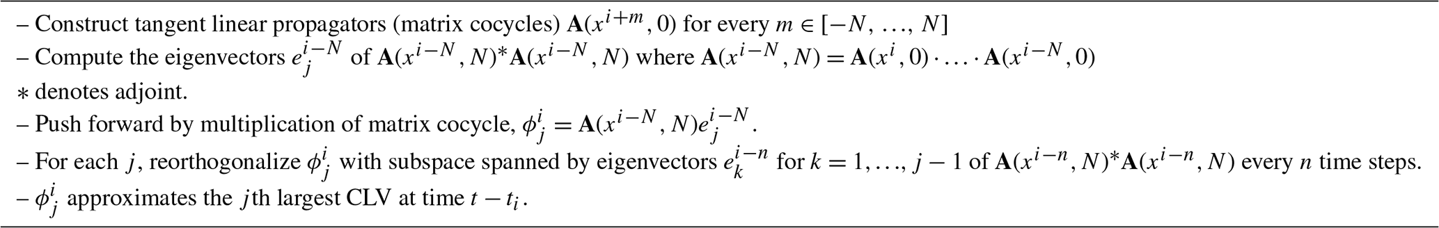
Ruelle (1979b) first described Oseledec splitting for invertible dynamics as the local decomposition of coordinate independent phase space into covariant directions of the Lyapunov vectors. Ginelli et al. (2007) introduced an algorithm to determine the set of points in phase space whose directions are invariant under time reversal and covariant with the dynamics arguing that these CLVs are coincident with the Oseledec splitting for any invertible dynamical system. A dynamical system is said to be hyperbolic if its phase space has no homoclinic tangencies; i.e., the stable and unstable manifolds are everywhere transversal to each other and that this is connected to hyperbolicity (Bochi and Viana, 2004). The determination of the angle between any given pair of CLVs allows for testing the degree of hyperbolicity at any point on the attractor where increasingly larger alignments indicates decreasing degrees of hyperbolicity and visa-versa. Many methods for calculating Lyapunov exponents are available, including recent machine learning approaches (Ayers et al., 2023). Here we use a QR decomposition to calculate the FTBLEs (Dieci et al., 1997; Van Vleck, 2010; Dieci et al., 2011). The computation of FTLEs over a finite window of time allows a time-dependent measure of the local unstable, neutral, and stable exponents of the evolving system which approach their asymptotic values as the window length increases.

Of interest here are the local dynamics of the respective chaotic attractors as measured in terms of their finite-time growth rates, hyperbolic splitting on the attractor tangent space (local manifold) measured in terms of alignment of the associated local Lyapunov vectors and dimensionality via the local Kaplan–Yorke dimension. The FTBLEs represent forward evolution over the past period defined by the chosen time window hence directly informing on how predictability varies on the attractor (Arbanel et al., 1991; Yoden and Nomura, 1993). Applying the QR decomposition over finite time windows optimizes mixed initial and evolved singular vectors such that they are no longer infinitesimal but are also of finite size where the chosen window enables exploration of the attractors multiscale nature. Of primary interest here is the application of methods for calculating covariant Lyapunov vectors to measure the degree of hyperbolicity in the local dynamics of the chaotic system.

As CLVs only truly exist in the asymptotic limit, FTCLVs are more correctly described as mixed initial and evolved singular vectors over some time window given a set of tangent linear propagators. Specifically, Oseledets (1968) theorem relates the Lyapunov exponents λ_i and a non-unique set of vectors ϕ via the forward and backward mapping of the tangent dynamics (cocycle) A(x(t),τ) as

$$\begin{array}{}\text{(1)}& {\mathit{\lambda }}_i=\stackrel{\lim }{\mathit{\tau }\to \mathrm{\infty }}{\displaystyle \frac{\mathrm{1}}{\mathit{\tau }}}\log \Vert \mathbf{A}\left(x\right(t),\mathit{\tau })\mathit{\varphi }\Vert \iff \mathit{\varphi }\in {\displaystyle \frac{{\mathrm{\Phi }}_i\left(x\right(t\left)\right)}{{\mathrm{\Phi }}_{i+\mathrm{1}}\left(x\right(t\left)\right)}}\end{array}$$

For the systems considered here, $\mathbf{A}\left(x\right(t),\mathit{\tau })={\exp }^{\mathit{\tau }\mathcal{J}f\left(x\right(t\left)\right)}$ where 𝒥 is the Jacobian of the right-hand side of any given systems of ODEs considered. For any given CLV pair, we define their alignment as ${\mathit{\theta }}_{i,j\in N}=|{\mathit{\varphi }}_i\cdot {\mathit{\varphi }}_j|/(\Vert {\mathit{\varphi }}_i\Vert \cdot \Vert {\mathit{\varphi }}_j\Vert )$. Correspondingly, ${\mathit{\theta }}_{i,j}=\Vert \cos \left({\mathrm{\Theta }}_{i,j}\right)\Vert$ given Θ_i,j is the angle between the ith and jth CLV, hence alignment is bounded between [0, 1]. For ${\mathit{\theta }}_{i,j}=\mathrm{0}$ the CLVs are orthogonal, and for ${\mathit{\theta }}_{i,j}=\mathrm{1}$ completely aligned.

To calculate the CLVs we employ Algorithm 2.2 of Froyland et al. (2013) described in Table 1. Following the algorithm, matrix cocycles are constructed and a singular value decomposition performed on each, after which the left singular vectors are sorted in descending order based on their singular values. The algorithm then performs a push forward operation over a defined window using the cocycle matrices then reorthogonalizing and repeating until we have a complete set of FTCLVs at a given point in time. For simplicity, we have used a common window δt for calculating the FTBLEs (window); FTCLEs (M_GR); and for the push forward cocyle window (M) used for calculating the CLVs i.e., $\mathit{\delta }t=\mathrm{window}=M_{\mathrm{GR}}=M$. For a more detailed discussion of the numerical algorithm see Froyland et al. (2013) and Appendix B of Axelsen et al. (2025). Throughout we use an orthogonalization step of 1.

We ascertain an approximation to the local attractor dimension based on either the FTBLEs or FTCLEs via the Kaplan-Yorke dimension (Frederickson et al., 1983; Kaplan and Yorke, 2006)

$$\begin{array}{}\text{(2)}& {\dim }_{\mathrm{KY}}:=j+{\displaystyle \frac{\sum _{i=\mathrm{1}}^j{\mathit{\lambda }}_i}{\left|{\mathit{\lambda }}_{j+\mathrm{1}}\right|}},\end{array}$$

where j is the largest leading eigenvector such that $\sum i={\mathrm{1}}^j{\mathit{\lambda }}_i\ge \mathrm{0}$ and $\sum _{i=\mathrm{1}}^{j+\mathrm{1}}{\mathit{\lambda }}_i<\mathrm{0}$.

3 Chaotic attractors

In the results to follow, ODEs, parameters, initial condition and integration timesteps for all chaotic attractors are described in Tables 2 and 3. The associated FTBLEs and FTCLEs for given cocycle windows are shown in Tables 4 and 5.

Table 2 Attractor definitions used in all subsequent figures and analyses.

Table 3 Attractor definitions used in all subsequent figures and analyses.

Table 4 Attractor FTBLEs and growth rates.

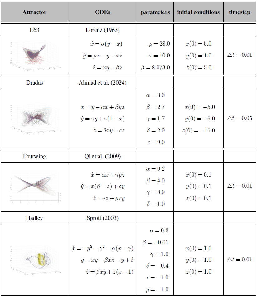
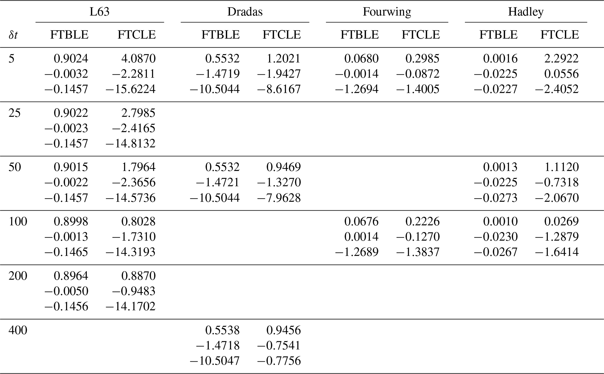
Table 5 Attractor FTBLEs and growth rates. Bracketed values indicate approximate asymptotic backwards Lyaponov Exponent (LE) values (δt=400) previously reported by Quinn et al. (2020).

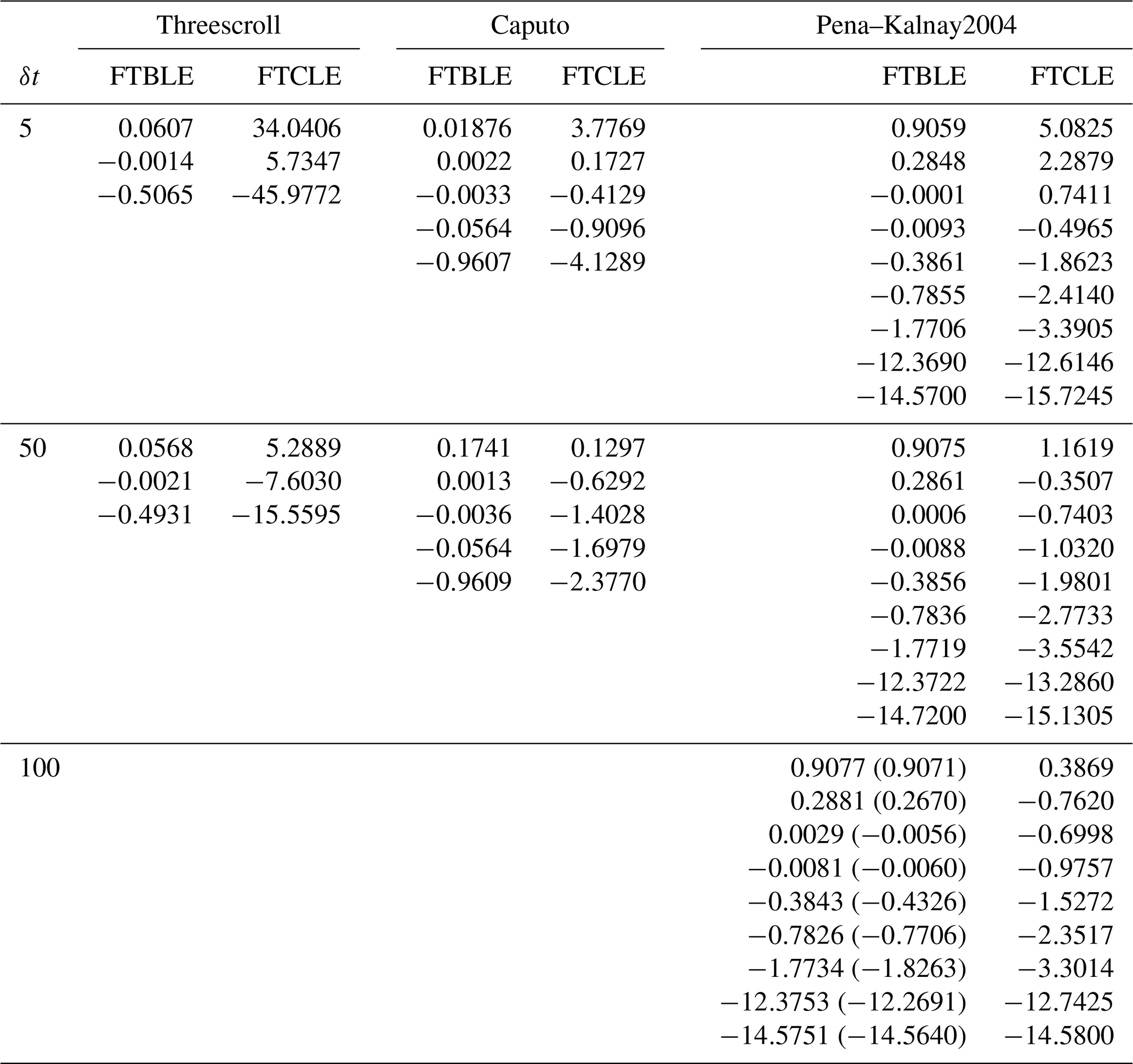
Figure 1 shows FTBLEs and corresponding instantaneous dim_KY values for the Lorenz “butterfly attractor” (Lorenz, 1963: L63) for windows δt=5, 25, 50, 100, 200. Figure 2 shows FTCLEs and corresponding dim_KY and in Fig. 3 we depict the alignment θ_i,j between the FTCLV pairs for each of the five chosen windows. The differences between FTBLEs and FTCLEs are immediately apparent most notably in the second exponent. In general, it is noticeable that where FTBLE1 is unstable, FTBLE2 is largely stable. FTBLE3 is always stable with the largest absolute values occuring where FTBLE1 is unstable. For cocyle windows δt=5, 25, 50, FTBLE1 is largely unstable in the region of the saddle and on a restricted region of the inner orbits of each wing of the attractor. As the window is increased to δt=100, unstable values are compressed to regions near the saddle and between the fast and slow orbits of the attractor wings. For windows δt>100 FTBLE2 assumes larger unstable values on the inner and outer loops. As window length increases the FTBLE3 values become increasingly less stable. The Fig. 1 dim_KY plots reflect the combined contributions of the FTBLEs to the attractor dimension. As forecast window increases the stable subregions evident at δt=5, 25, and 50 shrink where upon for δt≥100 the attractor is essentially unstable everywhere as expected. As δt→∞, dim_KY is seen to approach its asymptotic value at all points on the attractor.

Figure 1 L63: FTBLEs 1, 2, and 3 values at each point on the attractor in x-y-z orientation for windows δt=5, 25, 50, 100, 200. The far right column displays corresponding dim_KY values based on the instantaneous FTBLE values.

Figure 2 L63: as for Fig. 1 but for FTCLEs.

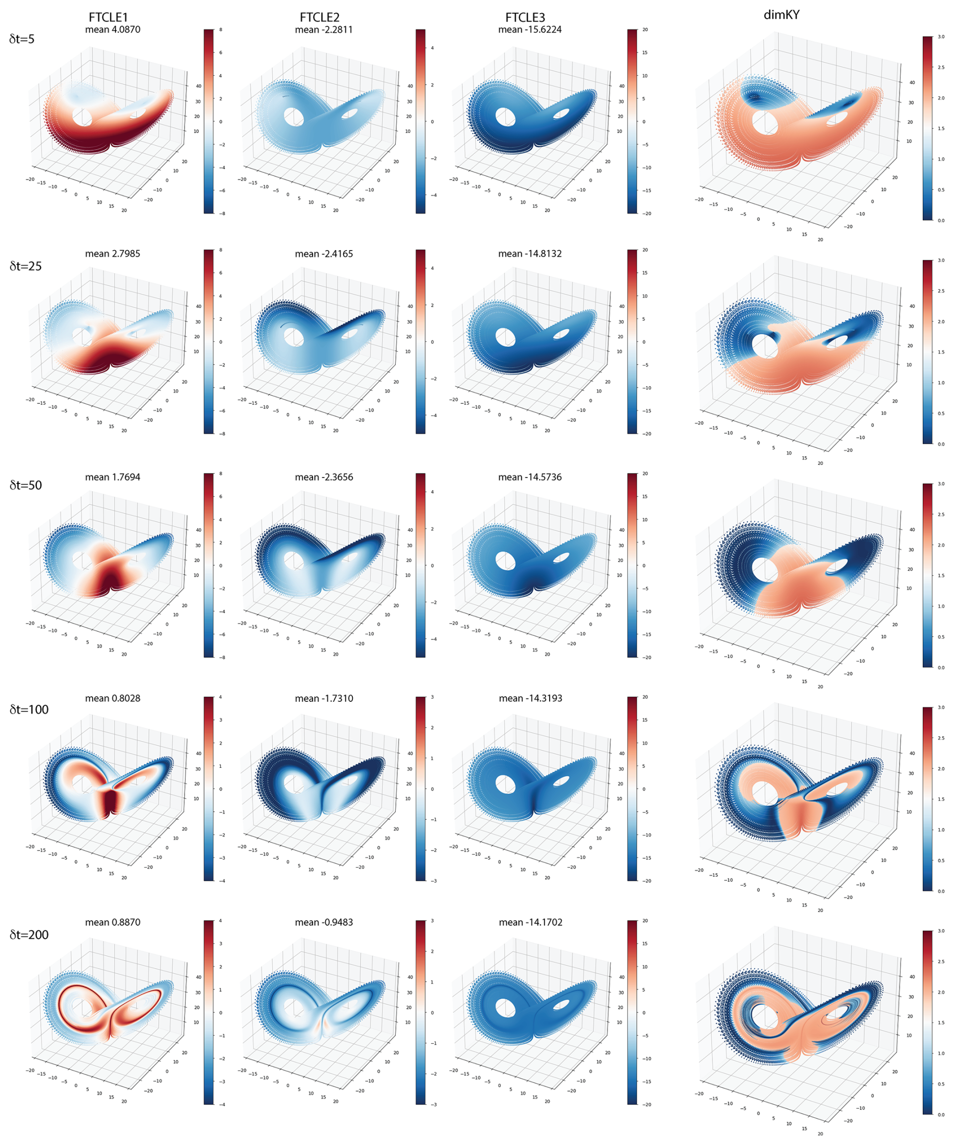
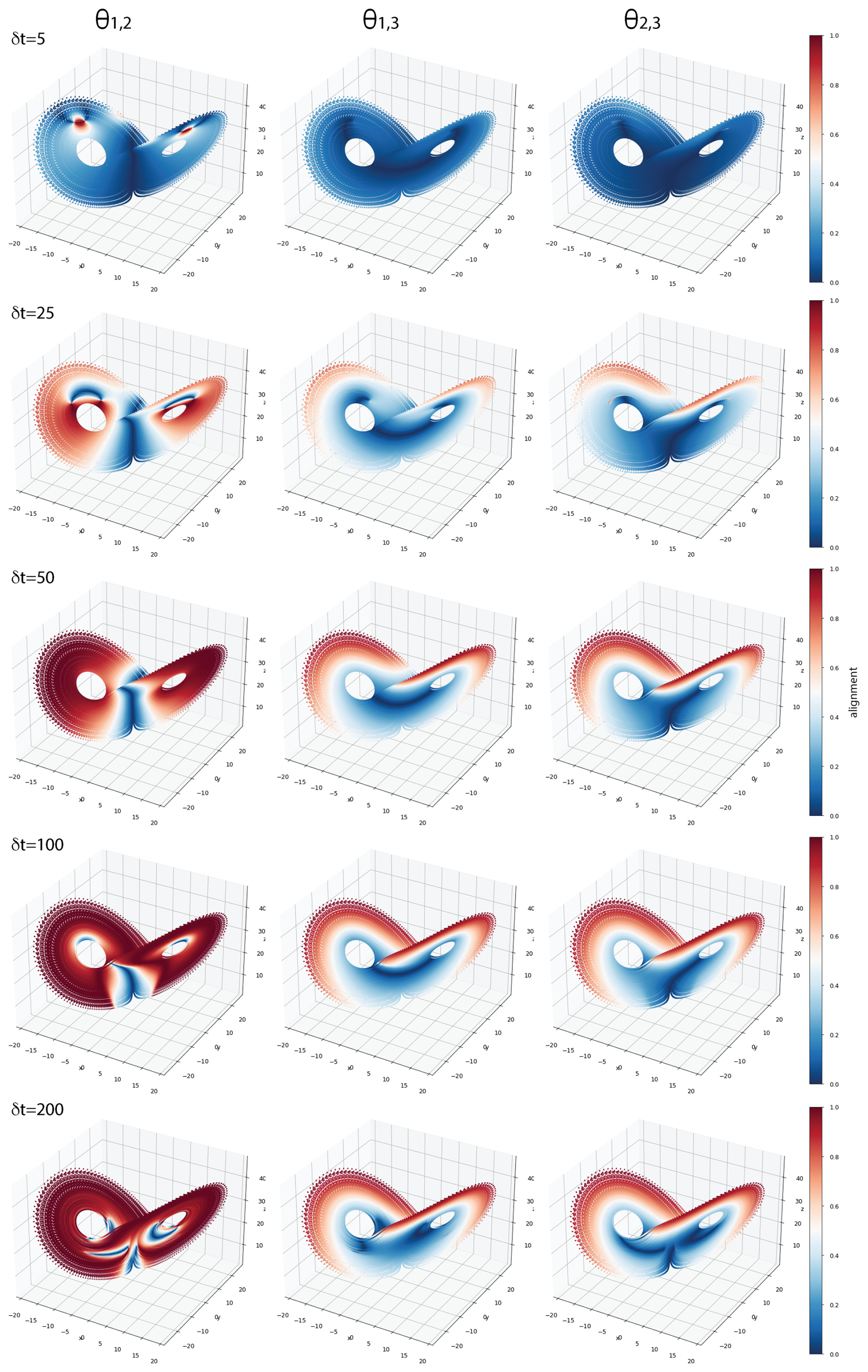
Figure 3 L63: θ_i,j pairs in x-y-z orientation. Values of 1 and 0 respectively indicate complete alignment or exact orthogonality.

The growth rate of FTCLE1 mirrors that of FTBLE1, however the stable subregions evident for δt=5 are considerably reduced in comparison. Further, we see (Fig. 2) FTCLE2 is stable and increasingly so in the outer loops as δt→100. However, at δt=200 the extent of the most stable regions of FTCLE2 reduces by ≈55 %. The FTCLE-based dim_KY largely reflects the subregion structure of FTCLE1 values on the attractor. In general, the mean values of the FTBLEs do not change appreciably however, those for the FTCLEs are highly variable. Considering θ_i,j (Fig. 3) we see the region of very low dimension evident in dim_KY for δt=5 (Fig. 2) corresponds very closely to the highly localized region of alignment evident between θ_1,2, otherwise there is minimal to no alignment elsewhere on the attractor. At δt=25 alignment near the same region becomes very low forming a locally hyperbolic subregion in addition to one near the saddle. As the window δt>25 increases, θ_1,2 alignment becomes ubiquitous in all regions away from the saddle. For δt=5, θ_1,3 and θ_2,3 exhibit values > 0.5 only on the same two subregions of the outer orbits of the attractor. For δt=100, 200, θ_1,3 and θ_2,3 values ≤ 0.5 correspond to subregions on the attractor where dim_KY>2.0 (Fig. 2). Hence at δt=200 it appears that regions with large FTCLE1 values i.e., >0.7, are permissible due to the correspondingly low alignments θ_1,3 and θ_2,3 compensating the high alignments θ_1,2.

Next we consider the three wing Dradas attractor. Dradas FTBLEs and FTCLEs are shown in Figs. 4 and 5 for δt=5, 50, and 400 respectively. Both FTBLE and FTCLE growth rates show very similar subregions for each of the considered values of δt. For δt=5 FTBLE1 and FTCLE1 two distinct unstable subregions are visible on two of the attractor wings while the third lobe is everywhere stable. FTBLE2 and FTCLE2 have similar corresponding regional structures although the unstable FTCLE2 subregions are more restricted relative to FTBLE2. FTBLE3 and FTCLE3 are stable everywhere on the attractor with mean values many times larger than that of the leading exponent signifying a highly extended system. At δt=50 the values of the leading exponent becomes unstable on the inner orbits of the attractor as those of the second exponent become stable. As δ→∞ all FTBLE and FTCLE values at any given point on the attractor approach their mean asymptotic value. While the mean FTBLE values are relatively unchanged as δt→∞, the absolute values of FTCLE2 and 3 reduce as they become increasingly less stable and the system less extended. Despite this the dim_KY values (Fig. 5) on the attractor are very similar regardless of being calculated using FTBLEs or FTCLEs. The Dradas alignments (Fig. 6) are substantially more complicated and less easily interpreted with respect to those observed for L63. However, for δt=5 we can recognize regions where all three FTCLVs are aligned such as the lower wing of the attractor, corresponding to stable subregions on the attractor with dim_KY values approaching zero. At δt=50 we see these subregions contract to distinct bands on the lobes after which the alignments θ_1,3 and θ_2,3 respectively break down becoming diffuse and unstructured at δt=400.

Figure 4 Dradas: FTBLEs 1, 2, and 3 values at each point on the attractor in x-y-z orientation for windows δt=5, 50, 400. The far right column displays corresponding dim_KY values based on the instantaneous FTBLE values.

Figure 5 Dradas: as for Fig. 4 but for FTCLEs.

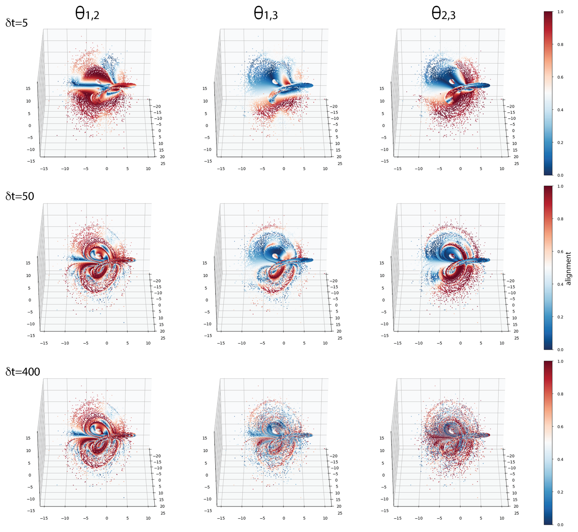
Figure 6 Dradas: θ_i,j pair values in x-y-z orientation with elevation angle 30° and azimuthal angle 0°. Values of 1 and 0 respectively indicate complete alignment or exact orthogonality.

The fourwing (Qi et al., 2009; Wang et al., 2010) and Hadley (Sprott, 2003) attractors for δt=5 are both hyperbolic at all points on the attractor with no stable subregions evident i.e., dim_KY>0 everywhere (Figs. 7 and 8). Both attractors show distinct FTCLE2 subregions of either growth or decay whereas those of the leading FTCLE1 are everywhere unstable and for the FTCLE3 everywhere stable. At δt=100 fourwing θ_1,3 and θ_2,3 alignments occur in the same localized outer regions of the attractor wings with the largest alignment values for θ_1,2 (Fig. 7). Fourwing dim_KY values resemble those of FTCLE2 being largest where FTCLE1 and 2 are coincidentally unstable and smallest where FTCLE2 and 3 are stable. Similar relationships between the growth rates and vector alignments occur for the Hadley attractor (Fig. 8) with one noticeable difference. For δt=100 we see the leading FTCLE1 indicate distinct regions of contraction and θ_i,j values correspondingly indicative of significant alignment between all vectors. In this case dim_KY>0.5 occur over a very restricted region where FTCLE1 growth rates are ≥0.75. FTCLE2 becomes everywhere stable with mean value approaching that of FTCLE3 hence determining the generally low dim_KY values.

Figure 7 Fourwing: θ_i,j values in x-y-z orientation with elevation angle 30° and azimuthal angle 0°. FTCLEs 1, 2, and 3 and dim_KY for δt=5, 100.

Figure 8 Hadley: FTCLEs, θ_i,j and dim_KY on the three dimensional projection of the attractor shown at δt=5, 100.

The threescroll attractor (Fig. 9) exhibits similar characteristics to those of Hadley and fourwing. At δt=5 the system exhibits low alignment values everywhere with nearly uniform growth rates at points on the attractor. FTCLE1 and 2 are everywhere unstable and FTCLE3 stable. This is reflected in dim_KY at points on the attractor are close to the average dim_KY≈2.5. At δt=50 mean values indicate contraction on most of the attractor as the ratio of $\mathrm{FTCLE}\mathrm{1}/\mathrm{FTCLE}\mathrm{3}\approx \mathrm{0.74}$ at δt=5 changes significantly to $\mathrm{FTCLE}\mathrm{1}/\mathrm{FTCLE}\mathrm{3}\approx \mathrm{0.34}$ as δt→50. Hence the system becomes more extended with regions of high dim_KY occurring where alignments θ_1,2, and to a lesser extent θ_1,3, are <0.5. The FTBLEs do not display this behavior with relatively small variations in mean values as δt is increased.

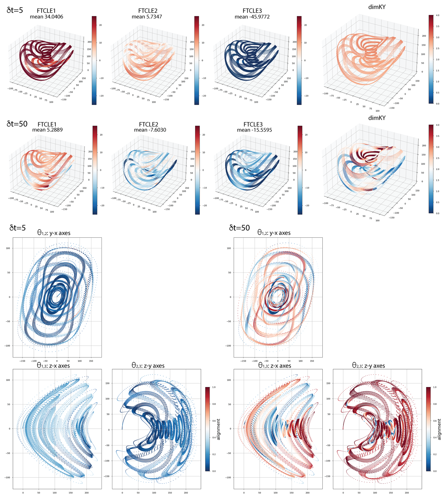
Figure 9 Threescroll: FTCLEs and dim_KY on the three dimensional projection of the attractor; θ_i,j pairs on chosen axes; shown at δt=5, 50.

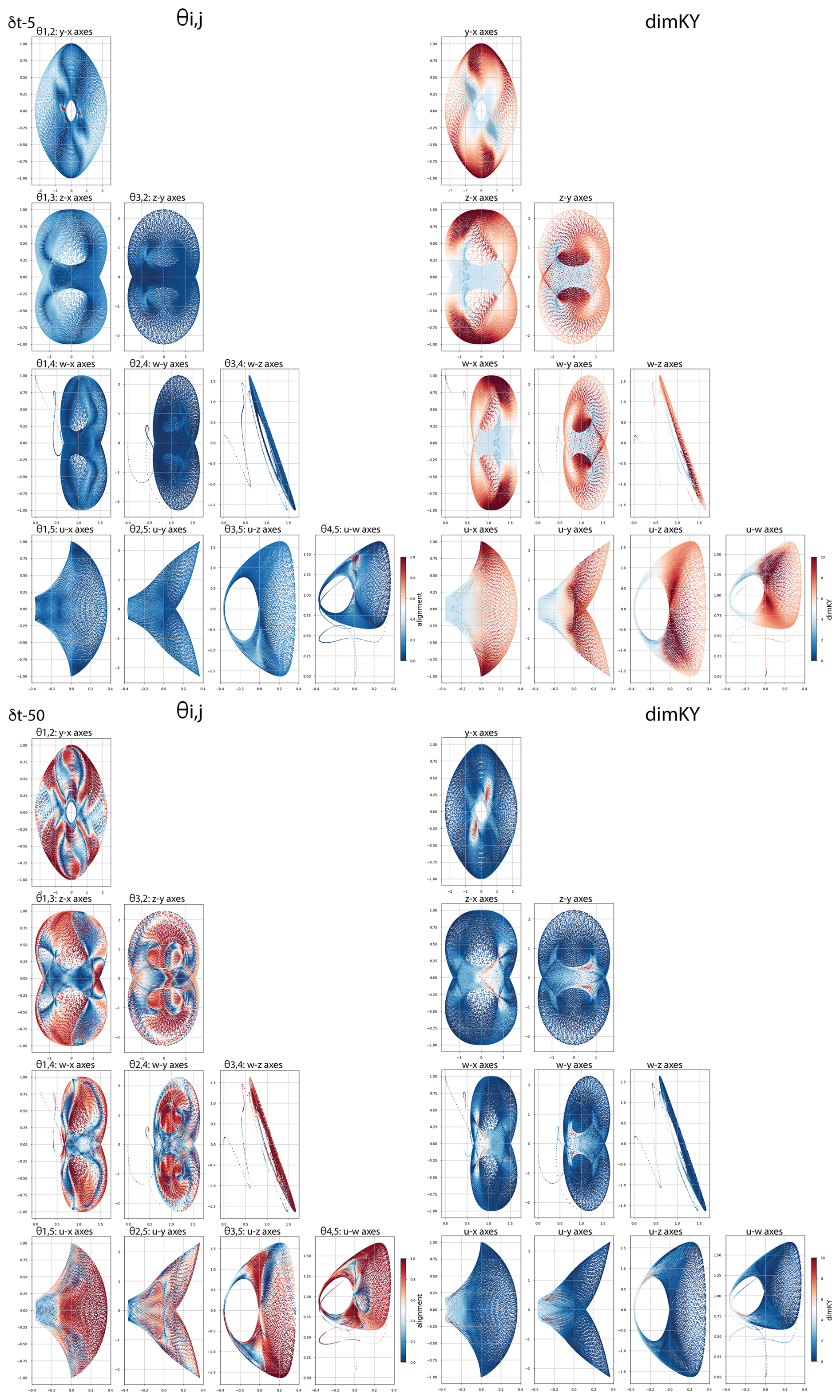
The five variable Caputo and nine variable Pena–Kalnay2004 attractors display very complicated relationships between alignment, growth rates and dim_KY. The Caputo attractor is hardest to visualize as, unlike Pena–Kalnay2004 which is comprised of three 3-component attractors coupled, it cannot be reduced to smaller coupled sub-models. As in the case for Fig. 9, in Fig. 10 we have chosen to visualize alignment and dim_KY in 2D on particular axes. At δt=5 the attractor alignments are approaching zero everywhere except for highly localized regions where θ_1,2 (x-y axis); θ_3,4 (w-z axes); and θ_4,5 (u-w axes) all approach 1.0. The relationship between alignment and dim_KY is less obvious than was observed in the case of the three-component systems, although we can recognize the attractor dimension is higher where dim_KY is large and the sum over the alignments small. In that sense, the relationship between transversality, hyperbolicity and local attractor dimension appears to hold as the dimension of the ODE system is increased.

Figure 10 Caputo: dim_KY for given θ_i,j pairs on chosen axes.

The Pena–Kalnay2004 attractor (Peña and Kalnay, 2004) has been employed previously in data assimilation studies by Yoshida and Kalnay (2018) and Quinn et al. (2020). The later study approximated the asymptotic Backwards Lyapunov exponents as averages over 400 time units with a timestep of 0.01 and orthogonalization step of 0.25, here shown as the bracketed values in Table 5. Quinn et al. (2020) and the earlier study of Vannitsem and Lucarini (2016), both found higher variability in the FTCLEs corresponding to the asymptotic neutral or near-zero valued modes. We find that increased variability of the FTCLEs relative to the FTBLEs is a general property of all exponents as evident from the values in Tables 4 and 5. While choosing to use the FTCLEs rather than the FTBLEs does lead to differences in the structure of the local Kaplan–Yorke dimension stable and unstable subregions, these differences are most evident in the relative magnitudes of the leading unstable and most stable exponents, and tend to diminish as δt→∞ as in the limit they approach the asymptotic LV values. Shown in the upper three rows of Fig. 11 dim_KY values calculated from FTCLEs are projected onto each of the three subsystems of the Pena–Kalnay2004 model. Here we see regions of high dimension contracting to the region of the saddle node  (x_e, y_e, z_e) and associated regions where alignments are generally small. The corresponding dim_KY values based on the FTBLEs at δt=100 are shown in last row in Fig. 11. Differences between FTBLE and FTCLE dim_KY values at δt=100 are largely in terms of the magnitude of the dimension with the most unstable regions occuring in co-located subregions i.e., differences correspond to a constant scale factor.

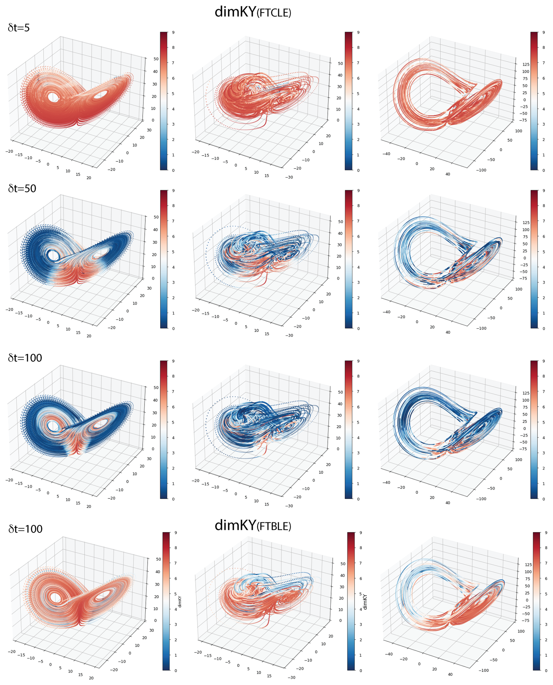
Figure 11 Pena–Kalnay2004: dim_KY at δt=5, 50, 100 on each of the three component subsystems (extratropical: x_e, y_e, z_e); (tropical: x_t, y_t, z_t); and (ocean: X, Y, Z).

4 Discussion and conclusions

Takeuchi et al. (2011) provide a framework for understanding hyperbolic decoupling of the tangent space into subspaces in high dimensional spatially extended dissipative systems in which the entangled “physical” modes are separated from the rapidly decaying stable modes. For prediction studies one is typically most concerned with the trajectory of the entangled modes on the associated finite-dimensional tangent space of the phase-space dynamics. This slow manifold is often identified in terms of the spectral gap in the eigenvalues. From the geometrical viewpoint, where the system is reducible to the evolution of a few degrees of freedom, it follows that the flow exists in a low-dimensional region of phase space, parametrized by a finite number of degrees of freedom. For geophysical fluids such as the atmosphere, one of the greatest challenges is to identify the emergence of a low-dimensional manifold in the local spatio-temporal dynamics of high dimensional flows. Such slow-fast hydrodynamic systems are paradigmatic examples with deep roots in statistical physics (Kogelbauer and Karlin, 2024).

Motivated by the work of Lorenz (1993) and Fraedrich (1986), as well as the questions posed by Ginelli et al. (2007), we have investigated hyperbolicity via the relationship between fluctuations of the Lyapunov exponents, transversality of their associated dynamical vectors, and dimensionality. We are further motivated by the recent study of mid-latitude persistent events in the Southern Hemisphere mid-troposphere by Axelsen et al. (2025). They employed an aggregated measure of alignment to indicate hyperbolic splitting of reduced local tangent space dynamics occurring at geographic locations where atmospheric blocking is known to preferentially occur (O'Kane et al., 2016). Here we undertook a more detailed examination of the local dynamics of a diverse set of chaotic attractors, some with characteristics broadly applicable to geophysical flows, to ascertain if commonalities exist.

Our general findings are:

• over short widows δt≤5 large hyperbolic subregions are present – sometimes over the entire attractor – where alignment between the leading dynamical vectors is very weak indicating a globally nearly hyperbolic system. In such cases the value of the leading exponent often solely determines the unstable subspaces indicated by the local attractor dimension. Additional highly unstable subspace regions distinct from those determined by the leading exponent, are generally associated with subregions where the near neutral exponents i.e., exponents whose asymptotic average values are near to zero, become locally unstable. The ratio of the absolute mean value of the leading unstable and the most stable FTCLEs is typically minimized i.e., $\min \left\{\frac{{\mathrm{FTCLE}}^{\mathrm{1}\mathrm{st}}}{{\mathrm{FTCLE}}^{\mathrm{last}}}\right\}$ for these short windows, an indication the system is at its most extended.

• over intermediate widows $\mathrm{5}<\mathit{\delta }t<\mathrm{100}$ the aforementioned unstable regions are observed to contract – often to those associated with a saddle however, absolute finite time exponent values in these reduced subspaces increase. The mean growth rates associated with the most stable exponents vary across the respective cases with some, like L63, remaining largely unchanged whereas others, like threescroll, becoming inceasingly less stable as δt increases. That said, the ratio of the absolute mean values of the most unstable to most stable exponents is most often observed to increase with window length. For the higher dimensional attractors Caputo and Pena–Kalnay2004, very complex alignments are manifest such that transversality between various vectors and exponent growth rates are complicated. In such cases the attractor dimension, which is an aggregated value of the exponents, is a more readily interpretable indicator of regions of (non)-hyperbolicity. The most complicated dynamics are observed to occur over these intermediate time windows.

• over extended widows δt≥100 the unstable subregion of the near neutral exponents evident at intermediate and shorter times tend to become stable on most of the attractor such that only the leading exponent determines regions where the unstable subspaces occur. As δt→∞ the values of a given exponent approach the mean asymptotic value at all points on the attractor and the subspace regions evident over shorter finite time windows merge and disappear. This is most easily seen for Dradas, the attractor with the most rapid convergence of the FTBLEs and FTCLEs to their mean asymptotic LE value.

Ginelli et al. (2007) proposed that access to the local directions of stable and unstable manifolds and the ready characterization and quantification of (non-)hyperbolicity affords a means to better model the spatial structure of the dynamics in extended systems. In particular, they note the key challenges to quantification of local measures of chaos and hierarchical modal decompositions of spatiotemporal chaos as well as the potential applications to prediction in nonlinear models. In recent years these ideas, including knowledge of the local transversality of invariant manifolds, have indeed been combined with linear and nonlinear generalizations of dynamical vectors using information on the past evolution e.g., SVs, FTBLVs, BVs, etc., to initialize optimal forecast perturbations along the relevant unstable directions determining error growth.

The chaotic attractors examined here represent paradigmatic examples of the dynamics of low dimensional physical systems. As mentioned in the introduction, L63 is derived as a three variable convective system. Similarly, the Hadley attractor is a reduced order model of the Hadley circulation i.e., the global-scale zonally oriented thermally driven cells within the troposphere that emerge due to meridional differences in insolation and heating between the tropics and the subtropics. The Pena–Kalnay2004 system is a reduced order paradigm model of interactions between tropical and midlatitude synoptic scale atmospheric variability and the ocean. The other systems considered all have aspects in their dynamics of relevance to geophysical flows and more generally to persistent properties in high dimensional systems associated with the emergence of a slow manifold. Emergent features in high dimensional flows are often described in terms of dynamics on a slow manifold. Frederiksen's three dimensional instability theory (Frederiksen, 1982, 1983) applies to atmospheric blocking (see also Zidikheri et al., 2006) providing a basis to understand the lifecycle of blocking in terms of growth rates of topographically trapped Rossby waves resonant with incipient baroclinic disturbances during onset; barotropic instability maintaining the structure during the coherent phase; and the re-establishment of baroclinic instability during decay. Using cluster analysis and an average measure of transversality as a proxy for mean hyperbolicity, Axelsen et al. (2025) recently showed that the mature phase of Southern Hemisphere blocking could be characterized by a small number of emergent low dimensional on average hyperbolic attractor states thus making a direct connection between instability theory and hyperbolicity.

The question arises as to the impact of increasing dimensionality. This goes to hyperbolic splitting, that is the separation of the physical modes from the fast decaying modes. For high dimensional systems, where scale separation exists, such as occurs where there is a distinct gap between low and high eigenvalues of the eigenspectrum, the slow manifold is easily determined and the influence of the fast decaying modes readily parameterized by a stochastic forcing. In the absence of stochastic forcing, a low order chaotic attractor, such as L63, in large part describes the dynamics of the slow manifold. Where multiple timescales are present, systems of ODEs where a fast attractor acts to force the slower modes, such as the slow-fast Pena–Kalnay2004 model, are instructive. That said, the analogy becomes weaker with increasing dimensionality and an absence of scale separation requiring more complete systems of equations to better describe the increased complexity.

Our study reveals that, even given the complexities of the local dynamics of low dimensional chaotic attractors associated with the manifestation of diverse unstable subspaces, there are general properties identifiable in terms of the relationship between transversality and local measures of chaos. We also note that the changing local hyperbolic structure can provide additional information about “nearby” (in parameter space) bifurcations potentially providing “early warning” indicators for tipping points, and that this is an area for further investigation.