NORAD tracking of the 2022 February Starlink satellites and the immediate loss of 32 satellites

In this work, North American Aerospace Defense Command (NORAD) tracking of the SpaceX Starlink satellite launch on 3 February 2022 is reviewed. Of the 49 Starlink satellites released into orbit, 38 were eventually lost. A total of 32 of the satellites were never tracked by NORAD. Two different physical mechanisms have been proposed and published in Space Weather to explain the satellite losses, while another mechanism has been proposed in a publication archived on arXiv. It is argued that none of these three papers can explain the immediate loss of 32 of the 49 satellites. We suggest that scientists use NORAD satellite tracking information to further investigate possible loss mechanisms.

1 Introduction

Geomagnetic storms (von Humboldt, 1808; Gonzalez et al., 1994) are caused by magnetic reconnection (Dungey, 1961; Tsurutani and Meng, 1972; Paschmann et al., 1979) between southward interplanetary magnetic fields (IMFs) and the Earth's dayside magnetic fields. The reconnected magnetic fields and solar wind plasma are convected to the midnight sector of the Earth's magnetosphere (magnetotail) where the magnetic fields are reconnected again (Dungey, 1961). The reconnected fields and plasma are jetted from the magnetotail towards the inner magnetosphere (DeForest and McIlwain, 1971), causing auroras (in both the northern and southern polar regions) (Akasofu, 1964) in the midnight sector at geomagnetic latitudes of 65 to 70° and slightly lower. The auroras also spread to all longitudes covering the Earth's magnetosphere at the above latitudes if the storm is intense and long-lasting.

These auroras are caused by the influx of energetic ∼ 10–100 keV electrons into the outer regions of the magnetosphere (Anderson, 1958; Hosokawa et al., 2020) and precipitation into the ionosphere, resulting in diffuse auroras, and parallel electric fields above the ionosphere accelerating electrons to ∼ 1–10 keV, resulting in discrete auroras (Carlson et al., 1998). The electrons impact atmospheric atoms and molecules at a height of ∼ 110–90 km, excite them, and decay, giving off auroral lines of violet, green, and red light. The influx of the energetic electrons also causes the upwelling of oxygen ions to heights at which they will affect orbiting satellites, causing enhanced drag on the satellites and eventual lowering of their orbits. This is the standard picture of low-altitude satellite drag during magnetic storms.

In 2022, three different scenarios were proposed to explain the unusual loss of many Starlink satellites. Before it was known that the Starlink satellites never reached their intended ∼ 500 km altitude, Tsurutani et al. (2022) proposed that prompt penetrating electric fields (PPEFs; Tsurutani et al., 2004, 2007; Lakhina and Tsurutani, 2017) could have been responsible for these losses. Their Fig. 2 (reshown here as Fig. 2) demonstrated that dayside near-equatorial density increases occurred at ∼ 500 km altitude during the two magnetic storms. However, the present orbital analyses indicate that none of the satellites lost on the first 2 d reached altitudes higher than 200 km for the entire orbit (and were, rather, still in elliptic trajectories). Thus, this loss mechanism must be discarded as a possible cause of the Starlink satellite losses.

The scenario put forward in Dang et al. (2022) also does not explain losses at such low latitudes. They used a global upper-atmospheric model (TIEGCM) to estimate the Joule heating by Ohmic dissipation at ionospheric altitudes. However, the Joule heating proposed by the authors was more remarkable at high latitudes, while the increases observed at latitudes below 53° were too small to create such an effect. Dang et al. (2022) also predicted losses in 5–7 d, assuming a constant 210 km satellite altitude. This cannot explain the possible immediate loss of the 32 satellites.

In contrast, Fang et al. (2022) used numerical simulations to show 50 %–125 % neutral density enhancements between 200 and 400 km. Their argument is based on the effects of Joule heating produced at high latitudes propagating to lower latitudes by large-scale gravity waves with phase speeds of 500–800 m s⁻¹ (Fuller-Rowell et al., 2008). This propagation may take 3–4 h and is, in addition to the effects of increased ultraviolet and extreme ultraviolet fluxes, due to the flares. Previous events had taken up to 30 h for the atmosphere to return to quiet conditions. We note, however, that Fig. 2 in the present work shows that there were very low Joule heating effects in the auroral zone during both of these magnetic storms, thereby negating the high-latitude Joule heating effects assumed in the model. Pitout et al. (2022) cast doubts that two rather small magnetic storms could have caused the Starlink satellite losses, in agreement with this paper. In 2023, Kakoti et al. (2023) proposed a new mechanism involving the “combined effects of neutral dynamics and electrodynamic forcing on the dayside ionosphere”. They concluded that minor storms can produce significant ionospheric variations over the American sector but did not comment on whether these changes could have caused the Starlink satellite losses. None of the above publications used information on the individual Starlink satellite orbits. In contrast, we have obtained North American Aerospace Defense Command (NORAD) tracking information for many of the individual satellites and will present our findings here. These results should be useful for modelers to understand the satellite loss mechanisms in more detail or for scientists to propose new loss mechanisms that have not been considered before.

2 Starlink launch

At 18:13 UT on 3 February 2022, SpaceX launched the Falcon 9 Block 5 rocket with the objective of deploying satellites for the Starlink Group 4-7, the sixth launch to the Starlink Shell 4 (Clark, 2022a, b). This launch received the COSPAR ID 2022-010. A video by Manley (2021) illustrates how two stacks of Starlink satellites could be put into orbit from a single launch vehicle. In this example, each stack of ∼ 30 satellites can be released in different directions. When the satellites separate from this stack, they start individual movements, sometimes colliding gently with others before entering into their individual flight orbits (Manley, 2021). For the 3 February launch, there were two stacks with 24 and 25 satellites in each stack. After the launch, the satellites may be put into edge-on directions with the solar panels parallel to the satellite bodies in an attempt to reduce drag. However, a telecommand is necessary to ensure that they maintain “safe-hold” mode, demanding some time and requiring some minimum antenna pointing (Clark, 2022b; McDowell, 2023).

The SpaceX mission that is the focus of this study was composed of 49 Starlink satellites that were initially planned to orbit the Earth at a ∼ 540 km circular low-Earth orbit (LEO). The initial planned elliptical orbit was 338 km × 210 km, at an inclination of 53.22° (Clark, 2022a). Once the initial elliptical orbits were obtained, SpaceX would use onboard propulsion to raise the orbits.

The 3 February deployment of the satellites occurred 15 min and 31 s after the liftoff, at a release time of 18:28 UT (Clark 2022a, b). SpaceX considered the launch successful, as satellite release occurred in the expected orbits, the rocket stage was recovered as planned, and all of the satellites were able to switch to autonomous flight mode.

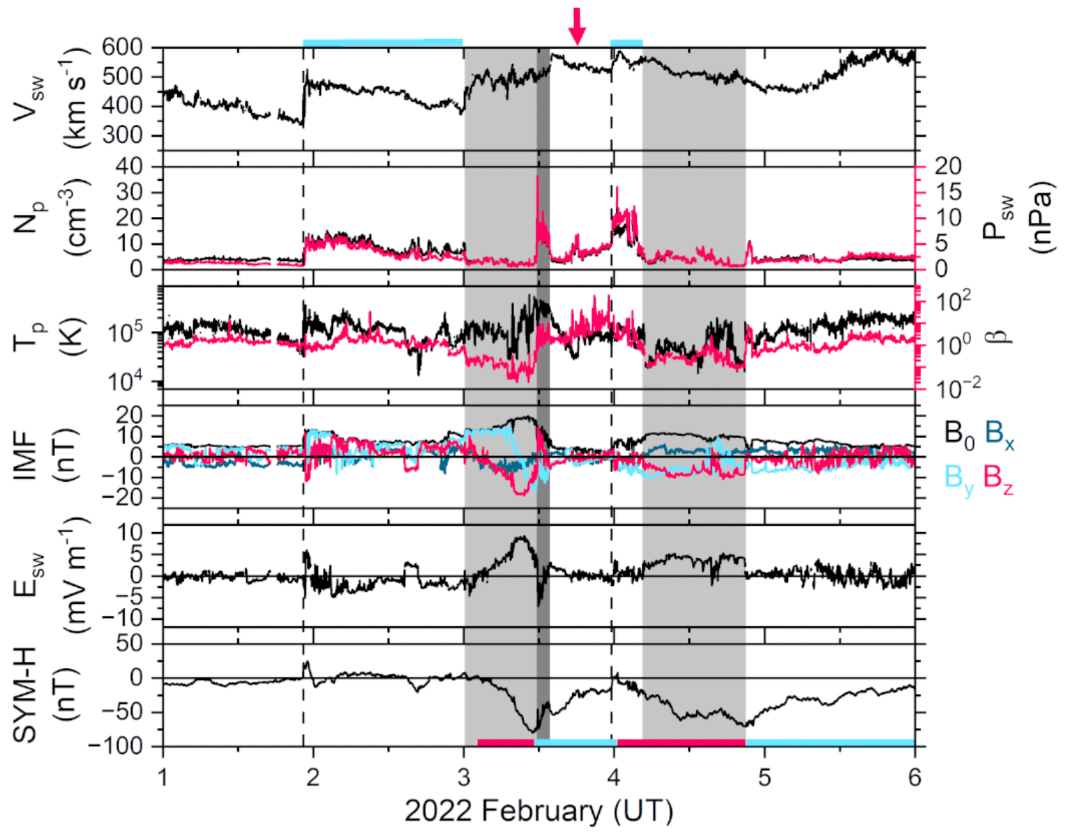
Figure 1 The interplanetary and geomagnetic conditions during the period from 1 to 5 February 2022. From top to bottom, the panels are as follows: the solar wind speed (V_sw); the plasma density (N_p; black, legend on the left) and ram pressure (P_sw; magenta, legend on the right); temperature (T_p; black, legend on the left) and plasma-β (magenta, legend on the right); the interplanetary magnetic field (IMF) magnitude B₀ (black), B_x (navy blue), B_y (cyan), and B_z (magenta) components; the electric field (E_sw); and the geomagnetic SYM-H index. The vertical dashed lines indicate interplanetary fast forward shocks. The light-gray shading indicates magnetic clouds (MCs), and the dark-gray shading indicates a solar filament propagated to 1 AU. Interplanetary sheaths are marked using cyan bars at the top. The figure is modified from Tsurutani et al. (2022). The arrow on the top of the figure indicates the Starlink satellites' launch time. The red and blue horizontal lines in the SYM-H panel indicate the storm main and recovery phases, respectively.

3 Space weather for the period

From the time of launch until a day after it, the near-Earth space weather conditions were disturbed: two geomagnetic storms occurred. For geomagnetic storm identification, we followed the classical definition of Gonzalez et al. (1994), who used the Dst index (equivalent to the SYM-H index used here) to identify a storm: when the index falls into the range between −30 and −50 nT for more than 1 h, it characterizes a small (weak) storm; events with decreases of between −50 and −100 nT for more than 2 h are considered a moderate storm; and an intense storm is one that results in Dst values of less than −100 nT for more than 3 h. The recovery phase is the interval during which the index begins to return to the values observed prior the storm; it may last from hours to several days. Figure 1 shows the interplanetary and geomagnetic conditions for the period of interest. The solar wind plasma and IMF data at 1 AU (astronomical unit) are time-shifted from the spacecraft location at the L1 libration point ∼ 0.01 AU upstream of the Earth to the nose of the Earth's bow shock. The IMF components are given in the geocentric solar magnetospheric (GSM) coordinate system. The solar/interplanetary data were obtained from NASA's OMNIWeb database (Papitashvili and King, 2020), whereas the storm-time SYM-H index was obtained from the World Data Center for Geomagnetism, Kyoto, Japan (World Data Center for Geomagnetism, 2022).

A few days prior to the Starlink satellite launch, on 29 January, an M1.1 solar flare erupted from active region (AR) 2936 at ∼ 23:00 UT. The flare can be seen in Geostationary Operational Environmental Satellite (GOES) X-ray data as a sudden increase in the radiation flux (NOAA, 2022). The activity in AR 2936 led to the release of a coronal mass ejection (CME) at 23:36 UT. Using the observed CME velocity near the Sun, the arrival of the CME at 1 AU was predicted. The geomagnetic impact of the interplanetary counterpart of the CME, or the interplanetary CME (ICME), was the occurrence of a moderate-intensity magnetic storm (Gonzalez et al., 1994; Echer et al., 2008) with a peak SYM-H intensity of −80 nT on 3 February. A second moderate-intensity geomagnetic storm with a SYM-H intensity of −71 nT occurred on 4 February.

The speed of the ICME at 1 AU was ∼ 500 km s⁻¹. This is classified as a moderately fast ICME (faster than the slow solar wind speed of ∼ 350–400 km s⁻¹). The fast ICME acted like a piston and caused an upstream shock and a sheath. The upstream fast forward shock reached the Earth at ∼ 22:19 UT on 1 February (indicated by a vertical dashed line in Fig. 1). The shock and sheath caused a sudden impulse (SI+) of 22 nT at the Earth's surface (Joselyn and Tsurutani, 1990; Araki, 1994; Tsurutani and Lakhina, 2014; Fiori et al., 2014; Lühr et al., 2009; Oliveira and Samsonov, 2018; Takeuchi et al., 2002), which is noted as an increase in the SYM-H index (the high sheath ram pressure in front of the fast ICME compressed the Earth's magnetosphere). The sheath following the shock did not contain major southward IMFs and was, therefore, generally not geoeffective (other than creating the SI+ and magnetospheric compression). The magnetic cloud (MC) portion of the ICME is identified (Burlaga et al., 1981, 1998; Tsurutani et al., 1988; Gopalswamy et al., 1998; Lepri and Zurbuchen, 2010; Sharma and Srivastava, 2012; Gopalswamy, 2015, 2022) by a high-IMF magnitude B₀ component and low plasma-β (the ratio between the plasma thermal pressure and the magnetic pressure) and is shown in Fig. 1 using light-gray shading. The MC extends from ∼ 23:54 UT on 2 February to ∼ 13:44 UT on 3 February. The IMF B_z component of the MC has the characteristic “flux rope” configuration with a southward component followed by a northward component. A flux rope is the geometry of magnetic fields in which field-aligned currents are flowing within the “magnetic rope” (Russell and Elphic, 1979; Yashiro et al., 2013; Marubashi et al., 2015).

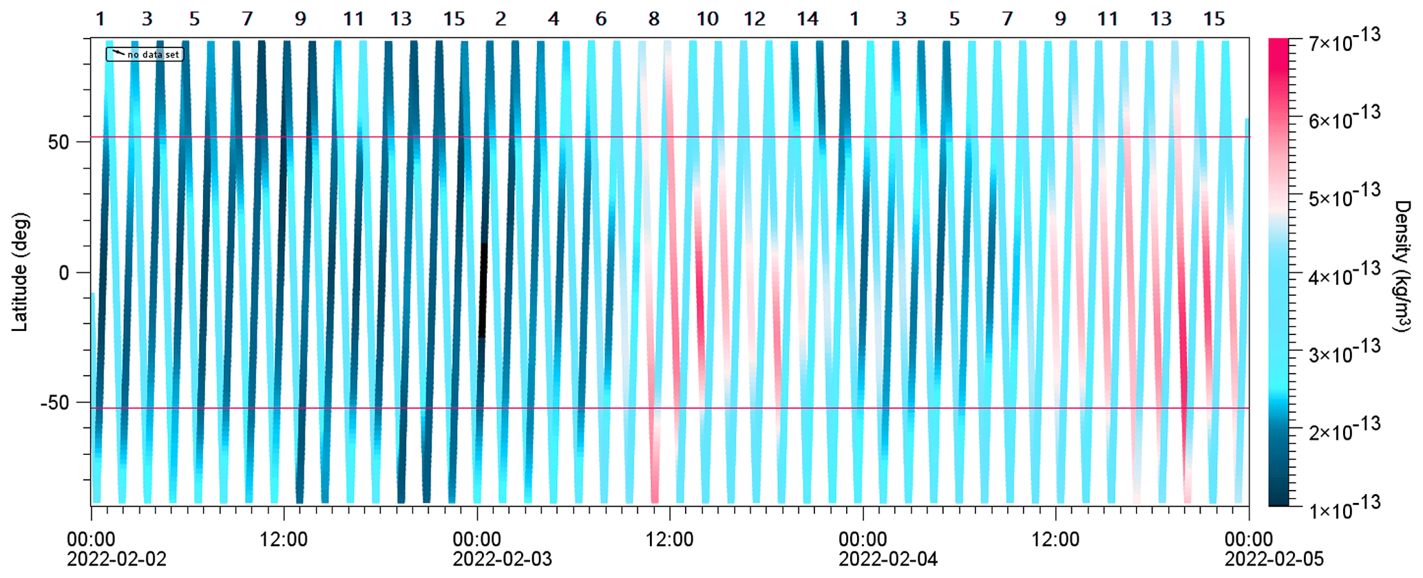
Figure 2 The Swarm B mass impact data for 2–4 February. The mass density is shown as a function of UT (x axis) and geographic latitude (y axis). It can be noted that the observations cover both day (north-to-south hemispheric passes) and night (south-to-north hemispheric passes) sides of the globe. The 2 February was a quiet day before the two magnetic storms and is shown as a “quiet-day reference”. The mass density values are given using a linear color scale on the right. Two red horizontal lines at +53° and −53° indicate the upper limits of the intended Starlink satellite orbits. Swarm B orbits on each day from the North Pole to the South Pole and back are marked by numbers from 1 to 15. Partial orbit 1 for 2 February is shown at the beginning of the figure.

During the southward IMF interval, the SYM-H index decreased to a peak value of −80 nT at ∼ 10:56 UT on 3 February. Thus, the magnetic storm is caused by the magnetic reconnection process between the interplanetary field and the Earth's magnetopause fields (Dungey, 1961). The dark-gray shaded region in Fig. 1 is the high-density solar filament portion of the ICME (Illing and Hundhausen, 1986; Burlaga et al., 1998; Wang et al., 2018; Kozyra et al., 2013). The filament also causes a compression of the magnetosphere and a sudden increase in the SYM-H index to −39 nT.

A second fast forward shock is identified at ∼ 23:37 UT on 3 February (marked by a vertical dashed line). The shock caused a SI+ of ∼ 17 nT. The following sheath did not contain any major IMF southward component and was, again, not geoeffective. The MC portion of the second ICME is indicated by light-gray shading from ∼ 04:37 to ∼ 21:02 UT on 4 February. The MC had a peak IMF B₀ of ∼ 12 nT at ∼ 08:02 UT. The MC B_z component profile is different from the previous MC. B_z is negative or zero throughout the MC. The negative B_z causes the second magnetic storm of peak intensity −71 nT at ∼ 20:59 UT on 4 February. There was no solar filament during this second ICME event. From Fig. 1, it is clear that SpaceX launched their Starlink satellites into a moderate-intensity magnetic storm. At the present time, it is unclear what the solar source (solar flare or prominence eruptions; Tang et al., 1989) was for this second ICME.

The effects of these storms on the atmospheric mass density are analyzed using data from the Swarm B satellite (Fig. 2). The Swarm mission is operated by the European Space Agency (Swarm, 2004). Swarm B is in a circular orbit at ∼ 500 km, with an inclination of ∼ 88° and orbital period of ∼ 90 min; thus, there are about 15 orbits per day. The orbits have been numbered for each day. At 00:00 UT on 2 February, the satellite was at ∼ −10° latitude at ∼ 09:00 LT (local time) on the dayside and was moving towards the South Pole. The mass density was ∼ 3.5 × 10⁻¹³ kg m⁻³ (light-blue color). Continuing in time as the orbit crosses over the South Pole and enters the nightside ionosphere at ∼ 20:00 LT, it is noticed that the density decreases to ∼ 1.5 × 10⁻¹³ kg m⁻³ between −53° and +53° (dark-blue color). The other orbits on 2 February show a similar pattern between the nightside and dayside passes.

During orbit 8 on 3 February, there is the first sign of a change (increase) in the mass impact at middle and low latitudes (∼ 5.0 × 10⁻¹³ kg m⁻³; pink color). This occurs at the South Pole crossing at ∼ 10:00 UT, just before the peak of the first magnetic storm. There is a density enhancement (red color) throughout this downward dayside pass, across the magnetic equator and to the South Pole. There is a local density maximum at ∼ 14:00 UT and ∼ 09:00 LT at 10° latitude. During orbits 9–13 on 3 February, the predominant density enhancements are on the dayside passes in the equatorial and midlatitude ranges. The enhancements are larger than those at higher latitudes. The maximum density of ∼ 5.5 × 10⁻¹³ kg m⁻³ occurred at ∼ 19:00 UT and ∼ 09:00 LT. This represents a density peak increase of ∼ 50 % relative to the quiet daytime density (2 February).

During orbits 9–13 on 3 February, the nightside equatorial and midlatitude densities are ∼ 3.5 × 10⁻¹³ kg m⁻³. This is higher than the 2 February (quiet-time) nightside densities of ∼ 1.5 × 10⁻¹³ kg m⁻³. Thus, during the magnetic storm, the nightside peak densities increased by ∼ 130 %. It is noted that the nighttime peak densities are less than the daytime peak densities. This latter feature will be explained later in this paper.

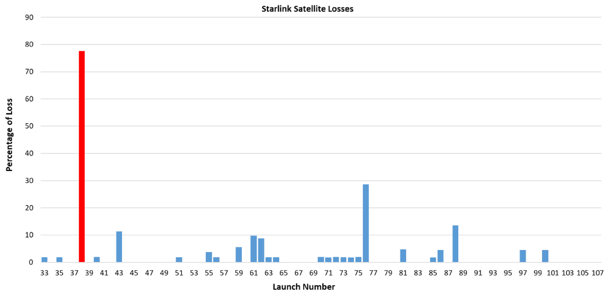
Figure 3 Percentage loss for Starlink launches no. 33 to no. 107. The event on 5 February 2022, marked as the red column in this plot, shows a failure rate of 77.6 %. The second-highest peak, launch no. 76, shows an unusual high-loss event, as this launch (Group 6-1) included several changes compared with the previous missions (including the first launch of larger Starlink V2 Mini satellites, the first use of an argon-fueled Hall-effect thruster in space, and changes in the tension rods to avoid releasing them in space).

The high-mass impact (red color) fades out by the end of 3 February and does not start again until orbit 8 on 4 February. A density peak of ∼ 5.3 × 10⁻¹³ kg m⁻³ in the equatorial region during orbit 8 occurred at ∼ 12:00 UT. This is approximately 10 h after the slowly developing second magnetic storm started at ∼ 00:15 UT on 4 February. From orbit 8 to 11, the predominant density enhancement occurs at the equatorial to middle latitudes, with little or no enhanced impact in the auroral/polar regions. The maximum density of ∼ 6.3 × 10⁻¹³ kg m⁻³ occurred at 20:00 UT on dayside pass 14 and extended to latitudes from ∼ −15° to −60°. The peak time is coincident with the peak in the second magnetic storm. On passes 15 and 16, the density decreases, and the enhanced density occurs mainly at the Equator and middle latitudes. The maximum density during this second storm event was ∼ 80 % higher than the dayside density values detected on 2 February.

The nightside density during orbit 14 on 4 February was ∼ 4.3 × 10⁻¹³ kg m⁻³. This is ∼ 190 % higher than the quiet-time value on 2 February. The nighttime peak densities are lower than the daytime peak densities, similar to the first storm features. The data for 5 and 6 February look similar to the quiet-day interval of 2 February; therefore, they are not shown to conserve space.

4 Magnetic storm effects on Starlink satellite survivability

Among the 49 released satellites, only 17 could be tracked by NORAD some days later. A total of 32 satellites were never listed by NORAD; thus, we assume that they were immediately lost after launch. This may have happened due to problems with tracking them (owing to extremely fast orbital decays in the first hours after their release or to substantially different satellite positions than expected for the launch).

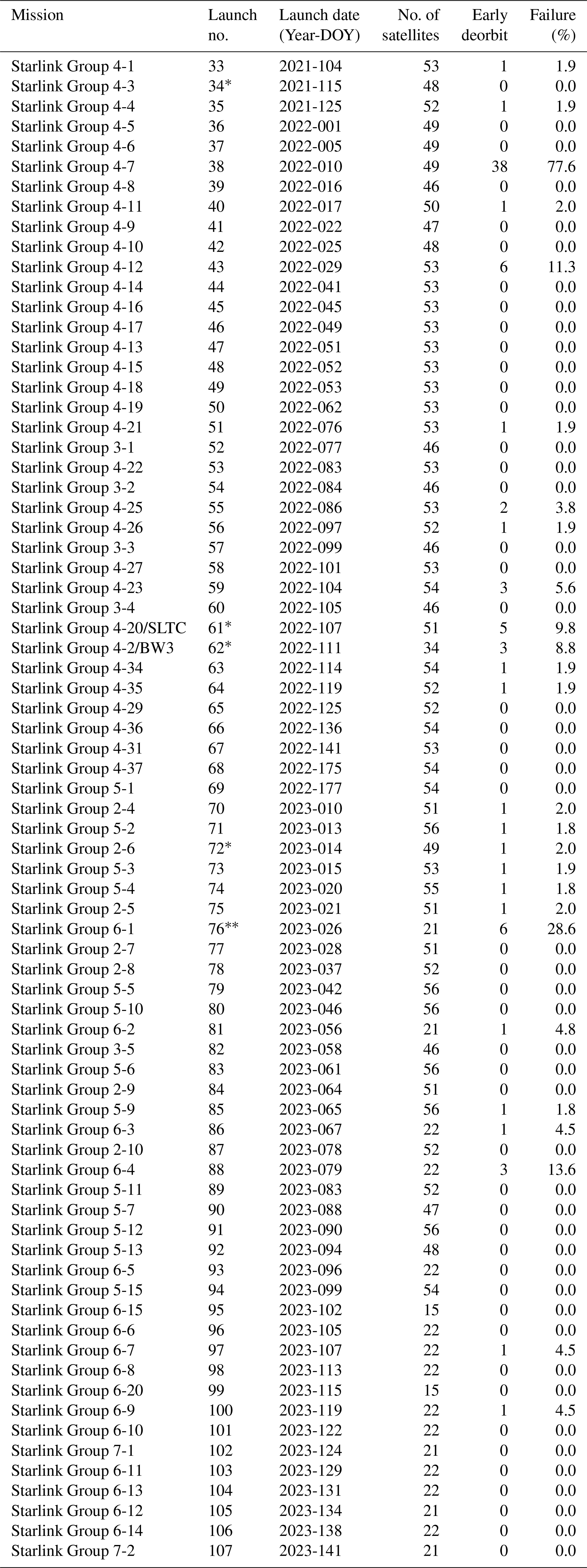
Considering the events since the start of the deployment of the Group 4 satellites, in 2021 November, the Starlink launch success rate has been around 97.5 % for the last 75 launches to date. However, the launch analyzed here, Starlink Group 4-7, represents a significant reduction in this efficiency, with an orbit insertion failure rate of 77.6 %. Figure 3 shows the percentage loss for Starlink launches no. 33 to no. 107. The event analyzed here is marked using a red column in the plot. The data used for this plot are available in Table A1 in the Appendix, which outlines the statistics of the launches for the 75 most recent Starlink satellite launches, up to 2023 September. For the calculation of the failure percentage, only satellites that failed during the orbit injection process were considered.

On 5 February, the tracking information for an initial group of four Starlink satellites was made available by NORAD. Two more satellites were tracked on 7 and 8 February. All of these satellites had very low perigees, ∼ 200 km altitude. The apogees were also very low: always below 350 km and even as low as 250 km in some cases. As the orbit injection velocities were too low for such unexpected low orbits, these satellites did not survive long and all of them reentered the atmosphere within a few days.

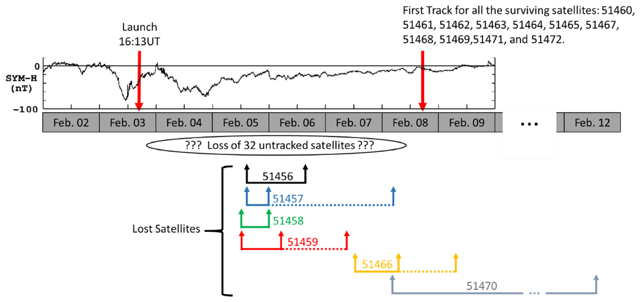
Figure 4 Timeline for the satellite tracking occurring between 2 and 12 February 2022. The plot shows the SYM-H index for the period from 2 to 9 February 2022. On the top of the plot, a red downward-pointing arrow (left) indicates the launch time, whereas a second arrow (right) indicates the beginning of the tracking of the 11 surviving satellites. At the bottom of the plot, the upward-pointing arrows in different colors indicate the beginning and end times of the tracking for each lost satellite. The oval indicates the time interval during which the 32 lost satellites were expected to be tracked.

A second group of 11 satellites were tracked some days later, on 8 February. These satellites were able to perform their ascending movements, changing from elliptical to circular orbits and rising to higher and more stable intermediate orbits at ∼ 350 km. The satellites were kept in this position for a few days. Afterwards, their orbits were boosted to their final altitudes of ∼ 540 km. However, one of these satellites, Starlink-3165 (NORAD no. 51471), displayed communication problems beginning on 31 October 2022. The satellite continued to be tracked in flight, but it was out of control and finally deorbited on 17 October 2023. The cause of this communication failure is still undisclosed; thus, it is not possible to verify whether it could be related to problems experienced during the first hours/days after launch.

5 Satellite tracking timeline

In order to make it easier to understand the entire sequence of events, a timeline was created that incorporates the space weather events, individual satellite tracking data, and other available information (see Fig. 4). The satellites are identified by their NORAD numbers. Only those tracked after 8 February were linked to their Starlink numbers.

Figure 4 shows a plot of the SYM-H index, which indicates the geomagnetic disturbances and the occurrence of geomagnetic storms. The two storm peaks are as follows: SYM-H = −80 nT on 3 February and SYM-H = −71 nT on 4 February. The red downward-pointing arrows indicate the launch times and the beginning of the satellite tracking for the 11 surviving satellites, respectively. It should be noted that the Starlink satellites were launched in the recovery phase of the first storm (SYM-H increasing from its minimum value). Thus, the satellites are expected to have experienced effects from the first magnetic storm. It is also noted that the second storm main phase started at the beginning of 4 February and continued for almost the entire day. Any Starlink satellites surviving the first storm would have experienced the effects of the second storm as well.

At the bottom of Fig. 4, the upward-pointing arrows indicate the beginning and end times of the tracking for all of the other lost satellites (besides the original 32 satellites that were never tracked). For satellites 51457, 51459, and 51466, the extended dashed line and another arrow indicate the “official” decay times. The oval indicates the time interval during which the 32 satellites were expected to be tracked but were already lost.

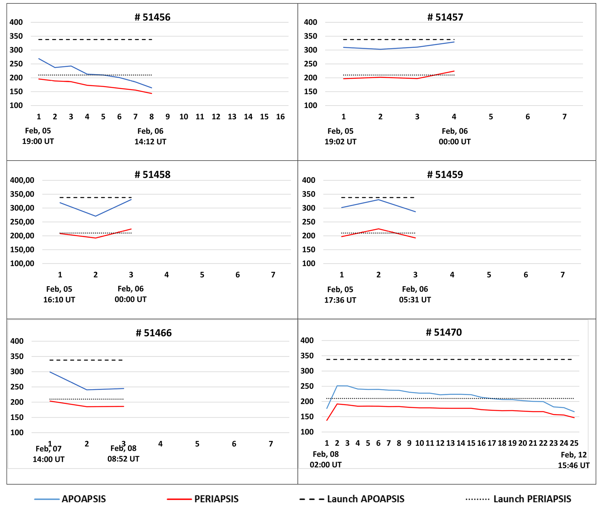
Figure 5 Panels showing the orbit perigees (red lines) and apogees (blue lines) for each of the decayed satellites. The vertical axis in each panel gives the satellite height, while the horizontal axis indicates the tracking sequence. The dates and times under the horizontal axis indicate the time of the first and the last tracking data. The two dashed black lines indicate the perigees and the apogees for the launch.

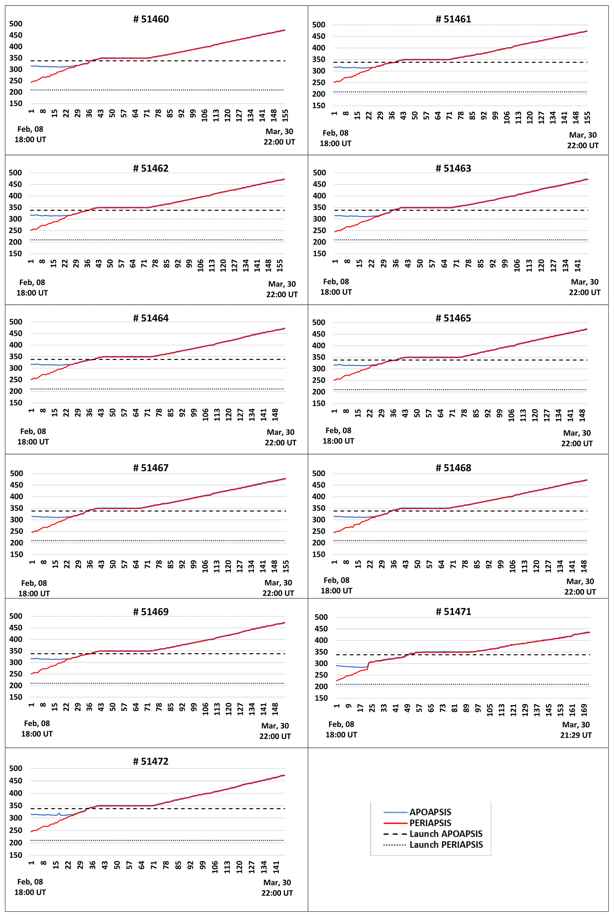
Figure 6 Panels showing the orbit perigees (red lines) and apogees (blue lines) for the surviving satellites. The vertical axes give the satellite altitudes (in km), while the horizontal axes indicate the tracking sequences from 8 February to 30 March 2022. The two dashed black lines indicate the perigees and apogees expected at the time of the launch.

6 Surviving satellite orbit information

Figures 5 and 6 show the orbit information for the decayed satellites and for the operational satellites, respectively.

In Fig. 5, the vertical axes give the satellite altitudes, while the horizontal axes give the tracking sequences. The two dashed black lines indicate the perigees and the apogees expected for the satellite launches, 210 and 338 km, respectively. The red and blue lines indicate the apogee and perigee at each tracking point. The date and time of the first and last tracking information are indicated under the horizontal axis.

For all of the above cases, the satellites were in very low orbits in the first track, close to the lowest orbits expected for the lowest perigees. The apogees were always very far (lower) from the expected values for the launch and sometimes even closer to the values expected for perigees.

It can be noted that some satellites started to rise in altitude, but most were likely lost due to insufficient thrust at such low orbits with increased atmospheric drag.

A contrasting scenario is shown in Fig. 6. All of these satellites survived the launch episode. After initial tracking by NORAD (all of them starting on 8 February 2022), they were boosted by onboard propulsion to safer (higher) altitudes. The plots are in the same format as in Fig. 5, but the horizontal axes now indicate the initial tracking (on 8 February) until 30 March.

It is interesting to note from Fig. 6 that all of the satellites started their orbits in elliptical configurations, with apogee and perigee values much higher than the (decayed) satellites shown in Fig. 5. The Fig. 6 satellite orbits were very close to the specified values for the launch.

The orbit shapes changed to circular configurations (indicated by the merging of the red and blue lines) with subsequent altitude increases to intermediate orbital configurations. Rising to the final orbits was done very slowly, and none of the satellites had reached the final ∼ 540 km altitude originally envisioned by 30 March, almost 2 months after the launch.

7 Discussion and conclusions

We have shown the available SpaceX Starlink satellite orbital plots as well as the sequence of events observed. The NORAD system was never able to identify 32 satellites. These satellites were presumably lost a few hours to a few days after launch. This implies possible quite heavy drag in the equatorial to midlatitude (up to 53° latitude) regions of the atmosphere at ∼ 200 km altitude. At the present time, there is not a known mechanism to cause such strongly enhanced drag at such low latitudes and altitudes.

Some of the satellites did survive the dual-storm event. As all of the Starlink satellites were launched at the same time and same altitude but had such widely varying fates (some being immediately lost and some surviving), it is clear that each one had a different flight history. This may have to do with the orientation of the satellite during its release (unknown), density pockets affecting stronger drag, or even satellite–satellite collisions during the release process. Electrostatic discharges (ESDs) were not considered, as SpaceX mentioned that the satellites were functional and communicating until the reentering the atmosphere.

It took several more days for NORAD to make the tracking information on another train of 11 other satellites available. The latter satellites were in more favorable positions (altitudes), allowing their recovery and rise to more stable orbits.

One can note from the above discussion that different satellites had extremely different orbital decay rates, indicating that one scenario cannot fit all 43 satellite cases. In particular, we are most concerned about the possible losses of 32 of the satellites within the first 48 h of launch, meaning that they could never be tracked by NORAD.

As mentioned in Sect. 1, Tsurutani et al. (2022) proposed that prompt penetrating electric fields (PPEFs; Tsurutani et al., 2004, 2007; Lakhina and Tsurutani, 2017) could be responsible for these losses. This hypothesis was discarded because the ionospheric plasma density changes (in percent) by PPEFs are effective at much higher altitudes, ∼ 500 km. We now know that the Starlink satellites never reached such altitudes. However, it was shown for the first time, using the Swarm satellite deceleration data, that storm-time PPEFs may be a main loss mechanism for satellites orbiting at ∼ 400–500 km altitudes. A referee of this paper asked the following question: “Could this PPEF mechanism cause high enough densities at lower (∼ 200 km) altitudes to create severe satellite drag?”. We think that this is improbable at such a low altitude; however, computer modeling would be useful to determine if a similar effect or a change in the local dynamics could occur at around 200 km.

Dang et al. (2022) used a global upper-atmospheric model (TIEGCM) to estimate the Joule heating by Ohmic dissipation at ionospheric altitudes but expected losses within 5–7 d, assuming a constant 210 km satellite altitude. However, the predicted loss timescales cannot explain the fast decay of the satellites within the first hours or days.

Fang et al. (2022) used numerical simulations to estimate increases in neutral density between 200 and 400 km at high latitudes due to Joule heating. In the Fang et al. model, the large-scale gravity waves (Fuller-Rowell et al., 2008) would propagate the effects to lower latitudes. However, there were very low Joule heating effects in the auroral zone during both of these magnetic storms, thereby negating the high-latitude Joule heating effects assumed in the model.

Using Super Dual Auroral Radar Network (SuperDARN) radar data, Walach and Grocott (2019) showed that ionospheric convection may expand to latitudes as low as 40° magnetic latitude in the ionospheric F-region (200–300 km altitude) during geomagnetic storms. This latitude is lower than the previously assumed limit for convection from the polar cap (typically 50° magnetic latitude). Although it is possible that the satellites may have crossed these regions when traveling through their highest latitude during orbit, this would be a relatively short interval of time compared with their orbital periods. Thus, we expect that this effect will be minor.

Kakoti et al. (2023) have suggested that significant morning–noon electron density reductions elucidated storm-induced equatorward thermospheric wind which caused the strong morning counter electrojet by generating the disturbance dynamo electric field. Substorm-related magnetospheric convection resulted in a significant noontime peak in the equatorial electrojet on 4 February. This is a very interesting possible explanation, but can it explain the near-immediate loss of 32 Starlink satellites?

Most of the existing published and under-review articles about these events have been based on modeling and simulations. The event outlined in this work represents a unique opportunity to utilize in situ observations from 49 satellites that experienced different conditions and fates. Although it is well known that private companies restrict the sharing of their telemetry data in order to preserve their technology, if Starlink could make a minimum dataset of telemetry data public, it would allow a multipoint-data-series analysis that would be useful to understand the physics behind this event. A dataset could provide the position of each satellite, their velocities and altitudes, some indication of whether the propulsion was active, and the solar panel's position. Even knowledge of a few satellites would be extremely useful.

Knowing the position of the satellites and their velocity profiles would indicate the region (in local time) in which the most intense drag increases occurred. That could be in the midnight sector, due to some effect of the magnetosphere tail reconnection, although this is not expected at such low latitudes for a moderate storm. The increases in the dayside could indicate some change in the ionosphere induced by electric field penetration (affecting not only the ionosphere but also the neutral particles). Tsurutani et al. (2004) has already demonstrated PPEF occurrence at higher altitudes (around 500 km); however, the plasma drag to higher altitudes may lead to the repopulation of other ions or even neutral particles at lower altitudes.

Even the possibility of collisions between satellites during the first moments after launch or whether the release direction played a role in the satellite fate could be confirmed or discarded by a quick analysis of their accelerometer/velocity data.

The velocity profiles along these inclined orbits could show us, via comparison among the satellites, whether there is a propagation of effects from high latitudes in the polar region to lower or middle latitudes. This analysis could also confirm the observations of Walach and Grocott (2019), who reported that auroral fluxes may expand equatorward during geomagnetic storms to as low as 40°, lower than the previously expected limited of 50° or higher. Moreover, these observations would help to understand whether these regions with increased drag were continuous regions or “tongues” of increased density as well as whether these phenomena could spread into all local times or are restricted to specific regions.

The present work makes it clear that the standard satellite drag computer codes are not able to predict the fast loss of 32 of the Starlink satellites. Perhaps including the possible nonlinearity of the atmospheric changes during disturbed geomagnetic periods could improve the codes' accuracy. Information on the satellite drag with the spacecraft orientation would help improve current models. Present models assume satellites with standard cross sections; however, the Starlink satellites are formed by two flat panels (the satellite body and the solar panel). Just after launch, the solar panel is folded on top of the satellite panel. During the period of orbital elevation, the solar panel is unfolded but kept aligned with the satellite body, becoming a long, flat panel. In the final position, the satellite assumes an “L” shape. This unusual shape of Starlink satellites makes their cross sections completely different from traditional satellites.

Future computer codes should take these different shapes and orientations into account and then calculate a maximum and minimum time for reentry. The codes should also consider satellite tumbling. Following these proposed changes, one could check if the computed loss times would be within the maximum and minimum satellite entry times or if they would be even greater.

8 Final comments

The losses of Starlink satellites in February 2022 were quite varied. Different satellites were lost at different times, whereas some satellites even survived. Clearly, a simple hypothesis involving an enhanced drag value is insufficient to explain the enormous variability in the different satellite responses. The most difficult problem is explaining the loss of 32 satellites within the first 2 d after launch. At this time, we do not have a physical explanation that involves the two magnetic storms. We hope to stimulate the scientific community to search for currently unknown physical mechanisms that might be able to explain such enormous drag occurring near equatorial regions at low altitudes. Such an event is a rare opportunity to have multipoint local data during a disturbed period and in a region where the satellites usually stay for a very short period of time before being propelled to their final and higher orbits.

It is also a remote possibility that the immediate 32 satellite losses were due to satellite–satellite collisions instead of or precipitated by increased drag during the magnetic storms.

The main result obtained from this study is that even a moderate storm may lead to losses when dealing with such low altitudes (at the limit of orbital conditions). The scientific community would greatly benefit if companies operating satellites in these low orbits could make a “scientific dataset” derived from their telemetry data public (while also protecting their sensitive information). The large number of satellites, which are almost evenly distributed across different latitudes and local times as well as at various altitudes (in a region where the satellites typically remain for a short period before being propelled to their final, higher orbits), would allow mapping of effects on their spatial distribution and their evolution (drift) over time. This would improve preparedness against space weather events and enhance our understanding of the physics in the ionosphere–mesosphere region during disturbed geomagnetic periods.

Appendix A

Table A1 Statistics of Starlink satellite launches from November 2021 (when Group 4 began to be deployed) to 12 September 2023, with the events ordered according to the launch date. The events marked with “^∗” indicate launches with another satellite in a rideshare configuration. The event marked with “${}^{\ast \ast }$” indicates the launch Group 6-1, which included several changes compared with the previous missions (including the first launch of larger, upgraded Starlink V2 Mini satellites with 4 times the bandwidth of previous models, the first use of an argon-fueled Hall-effect thruster in space, and changes in the tension rods to avoid releasing them in space) that may have increased the risk and number of failures. The table information was taken from McDowell (2023) and Wikipedia (2022).