Quantifying variability in Lagrangian particle dispersal in ocean ensemble simulations: an information theory approach

Ensemble Lagrangian simulations aim to capture the full range of possible outcomes for particle dispersal. However, single-member Lagrangian simulations are most commonly available and only provide a subset of the possible particle dispersal outcomes. This study explores how to generate the variability inherent in Lagrangian ensemble simulations by creating variability in a single-member simulation. To obtain a reference for comparison, we performed ensemble Lagrangian simulations by advecting the particles from the surface of the Gulf Stream, around 35.61° N, 73.61° W, in each member to obtain trajectories capturing the variability of the full 50-member ensemble. Subsequently, we performed single-member simulations with spatially and temporally varying release strategies to generate comparable trajectory variability and dispersal and also with adding Brownian motion diffusion to the advection. We studied how these strategies affected the number of surface particles connecting the Gulf Stream with the eastern side of the subtropical gyre. We used an information theory approach to define and compare the variability in the ensemble with the single-member strategies. We defined the variability as the marginal entropy or average information content of the probability distributions of the position of the particles. We calculated the relative entropy to quantify the uncertainty of representing the full-ensemble variability with single-member simulations. We found that release periods of 12 to 20 weeks most effectively captured the full ensemble variability, while spatial releases with a 2.0° radius resulted in the closest match at timescales shorter than 10 d. We found that adding relatively high amounts of Brownian motion diffusion (K_h=1000 m² s⁻¹) captures the entropy aspects of the full ensemble variability well but leads to an overestimation of connectivity. Our findings provide insights to improve the representation of variability in particle trajectories and define a framework for uncertainty quantification in Lagrangian ocean analysis.

1 Introduction

The ocean's dynamics, driven by atmospheric fluxes of energy and momentum at the surface, are characterized by phenomena that mutually interact across different spatiotemporal scales, including eddies, internal waves, zonal jets, and mixing processes, up to decadal and basin-scale fluctuations (Vallis, 2017). These multi-scale interactions are non-linear and difficult to model, presenting a significant source of uncertainty in ocean general circulation models (OGCMs) and our understanding of ocean circulation. Even under constant atmospheric forcing conditions, ocean models can produce divergent states from minimally perturbed initial conditions (Penduff et al., 2014). This intrinsic variability becomes particularly prominent in eddy-permitting models, where small initial differences can cascade towards multi-decadal and basin scales (Grégorio et al., 2015; Leroux et al., 2018; Zhao et al., 2023). To address these inherent uncertainties in OGCMs, researchers have increasingly adopted probabilistic ensemble models, running multiple simulations with small perturbations to initial conditions or parameter values to capture a broad range of possible ocean states (Penduff et al., 2018; Zanna et al., 2019). The ultimate goal of ensemble models is to predict the probability density of the system's state at a future time (Leutbecher and Palmer, 2008).

Lagrangian particle tracking provides a powerful tool for studying ocean transport, mixing, and connectivity, with the latter a metric that maps the origin of substances (water, nutrients, plankton, plastic objects) to their destinations. Applications of Lagrangian particle tracking range from search and rescue operations (Breivik et al., 2013) to climate and environmental research (Bower et al., 2019; Van Sebille et al., 2018). In these simulations, virtual particles are typically advected by velocity fields derived from OGCMs, with their dispersal patterns intimately linked to the underlying ocean state. However, similar to above, the trajectories obtained from the particle tracking in one OGCM ensemble member may not be representative of the full probability density of the system's state. Because pure advection is deterministic, there will be only one trajectory resulting from a virtual particle that starts at a certain place and time.

This deterministic nature limits what we define as “trajectory variability” – the range of possible pathways and end locations that particles could follow given uncertainties in ocean conditions. We define trajectory variability as the spread in particle positions, pathways, and connectivity patterns that emerges when accounting for uncertainties in initial conditions or modeled ocean states.

Capturing the trajectory variability is crucial for practical oceanography applications. For example, search and rescue professionals may want to compute a full probability density function of possible object locations – even when the starting location and time of an object lost at sea are known exactly – due to uncertainties in the ocean model. Similarly, marine pollution studies need to assess the range of possible contamination pathways, while connectivity studies in marine ecology require understanding the full spectrum of larval dispersal routes between habitats. In each case, a single deterministic trajectory provides insufficient information, limiting the generalizability of the results, as it cannot represent the inherent uncertainty in ocean dynamics and model predictions.

Now, advected particle trajectories are chaotic, in which small perturbations in initial conditions or noise along their trajectories can lead to significant divergences in particle trajectories (Koshel and Prants, 2006). The sensitivity to initial conditions is often used to generate variability in particle trajectories to predict the drift of the particles when there is uncertainty in their initial conditions (Breivik et al., 2013). In fluid mechanics, this is related to the concept of streaklines, transport barriers, and coherent structures (e.g., Haller, 2004; Zhang, 2013; Karrasch, 2016; Balasuriya, 2017).

An alternative approach to generating variability in the trajectories is to advect particles using a full ensemble of vector fields or ensemble models, an approach followed from Melsom et al. (2012), in which they advected particles using an ensemble of 100 members from the TOPAZ forecasting system. They found that ensemble average trajectories, calculated as the center of gravity (mean position) of all ensemble members at each time step, are generally closer (on a straight line distance) to the observed drifter trajectories than that from a deterministic single-member simulation. However, the study did not compare how small perturbations in initial conditions in the single-member simulation performed relative to the trajectories advected by the ensemble.

While ensemble Lagrangian simulations can capture a more complete spectrum of possible outcomes, single-member simulations, which sample only a subset of the possible outcomes, remain more prevalent due to computational constraints. In operational oceanography, data assimilative models are commonly used to improve trajectory predictions by combining observations with model dynamics to find an optimal solution (Castellari et al., 2001). However, while assimilation can reduce systematic biases and improve the mean state representation, it may not fully capture the underlying uncertainty and variability in particle trajectories, particularly in regions with sparse observations (Jacobs et al., 2018). Our study addresses these limitations by exploring ways of generating ensemble-like variability within single-member simulations. Missing variability in particle trajectories is typically created by releasing particles at different locations (spatial variation; e.g., Rossi et al., 2013), at different times (temporal variation; e.g., Qin et al., 2014; van Sebille et al., 2015), and/or with some random walk diffusion added to the advection (e.g., Hart-Davis and Backeberg, 2021). Here we test how well-suited these approaches are to represent intrinsic variability resulting from an ensemble simulation within a single simulation.

We assess performance based on a connectivity analysis and dispersion patterns using a novel information theory approach. Our approach consists of quantifying the variability in trajectories through the marginal entropy of particle position distributions and evaluating the uncertainty in representing full-ensemble variability with single-member simulations. Our approach is complementary to other new approaches for computing stochastic sensitivity of Lagrangian trajectories in the ocean, such as those by Balasuriya (2020), Badza et al. (2023), and Branicki and Uda (2023). However, our approach is particularly also useful for particles with added “behavior”, such as in the case of plastic particles (e.g., Denes and Van Sebille, 2024).

We focused on the region east of Cape Hatteras in the North Atlantic Ocean, implementing spatially and temporally varying release strategies to generate variability comparable to that observed in full ensemble simulations. This region was chosen to study the connectivity of water parcels at the surface of the Gulf Stream with the eastern North Atlantic and the subtropical gyre. It was previously thought that the salty and warm surface water of the Gulf Stream feeds directly to the subpolar gyre. However, recent Lagrangian studies have shown that the water parcels originating at the surface of the Gulf Stream recirculate within the subtropical gyre, becoming part of the subtropical mode water, and enter the subpolar gyre via sub-surface connections (Rypina et al., 2011; Burkholder and Lozier, 2014; Foukal and Lozier, 2016; Berglund et al., 2022). Our case study here thus builds upon these findings by quantifying how intrinsic ocean variability affects this connectivity pattern within the subtropical gyre, providing insights into the robustness and variability of these recirculation pathways.

2 Methodology

2.1 Ocean model ensemble simulation

We employed daily surface velocity fields produced by the North Atlantic NATL025-CJMCYC3 50-member ensemble simulation. This regional ensemble simulation was performed in the context of the OceaniC Chaos – ImPacts, strUcture, predicTability project (OCCIPUT), described in Penduff et al. (2014) and Bessières et al. (2017). This ensemble was performed using the NEMO v3.5 ocean/sea-ice model over the North Atlantic between 20° S and 81° N, with an eddy-permitting resolution of $\mathrm{1}/\mathrm{4}\mathit{°}$ and 46 vertical levels. The 50 ensemble members were initialized by the final state of a 15-year one-member spin-up that ended in December 1992. The inter-member dispersion was generated by activating small stochastic perturbations in the density gradients resolved by the model during 1993 and deactivating these perturbations for the remaining simulation time, as presented in Bessières et al. (2017) and based on the algorithm of Brankart (2013). All ensemble members were driven by the same atmospheric forcing between 1993 and 2015, derived from the DRAKKAR Forcing Set 5.2 (DFS5.2; see Dussin et al., 2016). The NATL025-CJMCYC3 1993–2025 simulation used here is similar to the NATL025-GSL301 1993–2012 simulation presented in Narinc et al. (2024), with one difference: tropical cyclones were enhanced in the forcing of NATL025-CJMCYC3 since they were too weak in DFS5.2. More details about the model setup are provided in Narinc et al. (2024).

2.2 Lagrangian simulations

Lagrangian particles were advected offline using 6 years (2010–2015) of the velocity fields described above, where particle trajectories in each ensemble member were integrated using the Parcels framework v.3.0.2 (Delandmeter and van Sebille, 2019). Trajectories were integrated in three dimensions using a fourth-order Runge–Kutta scheme with a time step of 1 h, storing the output with a daily time step. We modeled passive particles (that is, particles that instantly adjust their velocity to that of the ambient flow) by only considering three-dimensional advection and ignoring all buoyant forces. Additionally, particles that escaped the domain through the surface were placed back to a depth of 1 m. We chose the region off the coast of Cape Hatteras as a study location because it is an important region where the Gulf Stream separates from the continental shelf and becomes a free jet (Mao et al., 2023; Buckley and Marshall, 2016).

2.3 Recreating particle trajectory variability

This study explores methods to recreate the trajectory variability typically obtained from ensemble ocean simulations using only a single ensemble member. Figure 1 illustrates both the challenge and our proposed approaches. When particles are released from a fixed point (35.61° N, 73.61° W; yellow square) at a distinct time (2 January 2010) and tracked using different ensemble members, their trajectories (shown in black, Fig. 1A) diverge due to intrinsic variability in the velocity fields. Our goal is to reproduce this dispersion of what we refer to as the “full ensemble” using just one ensemble member.

We tested three approaches to achieve the variability of this full ensemble with single-member simulations, by leveraging the sensitivity to initial conditions or adding diffusion. The first strategy varies the release locations of the virtual particles spatially (shown in purple in Fig. 1B), creating a cloud of initial positions centered around 35.61° N and 73.61° W. The purple circles indicate the varying release locations, while the purple arrows show their subsequent trajectories. The second strategy (shown in orange, Fig. 1C) maintains the fixed release location (yellow square) but varies the release timing, with particles released continuously over a time period. The third strategy (shown in green, Fig. 1D) maintains the fixed release location and release time but adds a small Brownian motion diffusion to the trajectory simulations. All methods generate trajectory spreading with different patterns, some of which qualitatively resemble the full ensemble trajectories, which we seek to quantitatively compare.

The single-member simulations were performed using velocity fields from individual members of the NATL025-CJMCYC3 ensemble. To ensure robust statistics, we repeated each strategy (spatial and temporal variation and added diffusion) with all 50 ensemble members rather than arbitrarily selecting one. For the ensemble simulations, rather than running new simulations where all ensemble members simultaneously advect particles, we selected and joined trajectories from our existing single-member simulations to create a “synthetic” mixture-of-all-member simulation. This mixture simulation contains the full ensemble variability and is our benchmark for comparing the three single-member strategies. The following subsections further detail the three single-member release strategies and the ensemble simulations, which we refer to as mixture simulations.

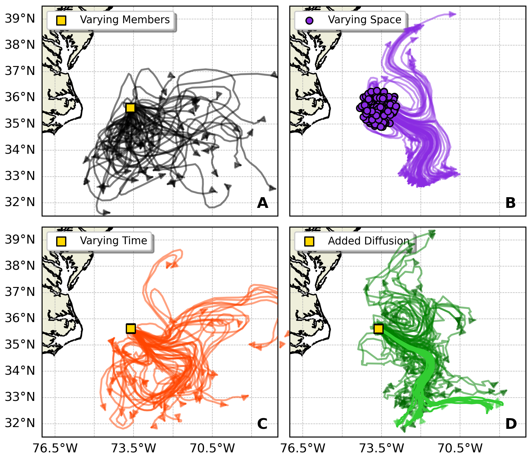
Figure 1 Schematic representation of the experiment design, east of Cape Hatteras, showing four approaches to generate variability in the particle trajectories. (A) The black lines show 50 trajectories of particles released from a single point (35.61° N, 73.61° W; yellow square) at a distinct time (2 January 2010) and advected using velocity fields from all 50 members of the NATL025-CJMCYC3 ensemble. (B) Purple trajectories show 50 randomly selected particles, out of 7500, released from spatially varying locations (purple circles) within a 1° radius of the central point, all advected using ensemble member 3. (C) Orange trajectories represent 50 randomly selected particles, out of 7500, released uniformly over a 20-week period from the central point (35.61° N, 73.61° W; yellow square), also using ensemble member 3. (D) Green trajectories represent 50, out of 7500, randomly selected particles from the ensemble member 3 simulation with low diffusion (K_h=10 m² s⁻¹; light green) and high diffusion K_h=1000 m² s⁻¹; dark green), released from the central point (35.61° N, 73.61° W; yellow square). All trajectories are shown 35 d after their respective release times.

2.3.1 Spatially varying release

We performed Lagrangian simulations by releasing a cloud of particles around (35.71° N, 73.61° W), at 1 m depth, on 2 January 2010 and tracking them until the end of 2015, so for 6 years in total. We evenly spaced the particles in concentric rings around the coordinates, where each ring was placed at a constant radial separation (δ_r) from the prior ring, forming a circle of particles. We varied the radius of this cloud of particles; the larger the radius, the less correlated the velocity vectors of the particles are expected to be, creating more variability in the trajectories. The choice of spatial release radii (9–180 km) spans the range from subgrid scales to 10 grid cells apart, allowing us to test how initial condition uncertainties at different (grid) scales affect long-term particle dispersion. We created three sets of simulations, with 50 simulations per set (one per ensemble member). The three sets of simulations were performed with 7500 particles, with an initial cloud varying ${\mathit{\delta }}_{\mathrm{r}}\in \mathit{\{}\mathrm{0.1}\mathit{°},\mathrm{1.0}\mathit{°},\mathrm{2.0}\mathit{°}\mathit{\}}$.

At the release point, the initial cloud radii are approximately 9, 90, and 180 km. As a reference, we computed the ensemble average spatial autocorrelation function of the initial particle velocities at the release location on the release day (2 January 2010). The spatial autocorrelation function describes the average agreement between a pair of particle velocities separated by a distance L. The larger the separation distance L, the more likely their velocities will be decorrelated (LaCasce, 2008). Assuming that the spatial correlation decays exponentially, we defined the decorrelation length scale L_L as the e-folding length scale of the exponential that describes the autocorrelations functions (Xia et al., 2013).

The particle-pair spatial autocorrelation function was calculated over a set of points placed over a west-to-east line, shown by the blue dots in Fig. 2A, with a horizontal spacing of 0.01°. We calculated the velocity autocorrelation function from these points as a function of the distance L. The spatial autocorrelation function is defined as

$$\begin{array}{}\text{(1)}& \mathit{\rho }\left(L\right)=\langle {\displaystyle \frac{\mathit{u}(r_{\mathrm{0}}+L)\cdot \mathit{u}\left(r_{\mathrm{0}}\right)}{\Vert \mathit{u}(r_{\mathrm{0}}+L)\Vert \Vert \mathit{u}\left(r_{\mathrm{0}}\right)\Vert }}\rangle ,\end{array}$$

in which we compute the dot product of a pair of vectors u(r₀) and u(r₀+L), divided by the multiplication of their norms, averaged over all the pairs of velocities (Xia et al., 2013). In Eq. (1), $\Vert \cdot \Vert$ is the usual L₂ norm, and 〈⋅〉 indicates an average over velocity pairs. We computed ρ(L) for the range $L\in [\mathrm{0.01}\mathit{°},\mathrm{2.00}\mathit{°}]$, with a 0.01° spacing. The autocorrelation function is defined between $[-\mathrm{1},\mathrm{1}]$, in which ρ(L)=1 indicates a full positive correlation, $\mathit{\rho }\left(L\right)=-\mathrm{1}$ a full negative correlation, and ρ(L)=0 no correlation.

Following Eq. (1), we computed ρ(L) for each of the 50 ensemble members of the NATL025-CJMCYC3, on 2 January 2010. In Fig. 2B, we show the ρ(L) for each ensemble member as black lines. We see great variability in the curves but an exponentially decaying trend in which, as L increases, the particle velocities are less correlated. We performed an exponential fit, $e^{x/L_{\mathrm{L}}}$, of the 50 correlation curves, shown in blue in Fig. 2B. From the exponential fit, we obtained a decorrelation length L_L=0.41°, which corresponds to approximately 37 km at a latitude of 35.5° N. Both spatial scales indicate that the velocities of all the particles released from an initial cloud of δ_r=0.1° should be correlated, while for the larger clouds ${\mathit{\delta }}_{\mathrm{r}}\in \mathit{\{}\mathrm{1.0}\mathit{°},\mathrm{2.0}\mathit{°}\mathit{\}}$, only a fraction of the particle velocities may be correlated, leading to more variability in the trajectories. While decorrelation scales likely evolve over the 6-year simulation period due to particle spreading and varying flow conditions, computing their evolution at every particle age is computationally intensive and impractical, compared to other metrics.

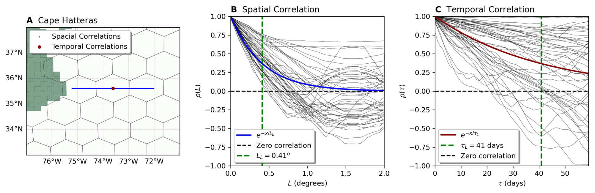
Figure 2 (A) Map of Cape Hatteras showing the points used to compute the spatial correlations (blue) and the location used to compute the temporal correlations (red). The hexagons mark the limits of the hexagonal grid used in subsequent analyses, and the green area represents the North American coast. (B) Spatial correlations function around the release location, and each black line shows the correlation function for an ensemble member. The blue line shows the exponential fit computed over the 50 correlation functions. The green line shows the decorrelation length scale $L_{\mathrm{L}}=\mathrm{0.41}\mathit{°}\approx \mathrm{37}\mathrm{km}$. (C) Temporal correlations with velocities sampled daily for 60 d from 2 January 2010. The black lines show the correlation functions of single ensemble members, and the red line shows the exponential fit with a decorrelation timescale of 41 d.

2.3.2 Temporally varying release

We also created variability by releasing particles from the same location (35.71° N, 73.61° W) at different times. We tested three release time windows, 4, 12, and 20 weeks, all starting from 2 January 2010. For each window length, we performed 50 simulations (one per ensemble member), with each simulation releasing 7500 particles. Within each time window, we distributed the 7500 particles evenly across the days, resulting in multiple particles being released each day. To ensure particles released on the same day followed different trajectories, we added small random perturbations to their release locations using uniform noise with an amplitude of 0.01°. We kept this noise amplitude small to (as much as possible) isolate the effects of the temporal release strategy alone. Note that all particles were advected until the end of 2015, so that in this simulation some particles reached a maximum “age” (time of flow) of 6 years and others only 5.6 years. This is a minor effect though, as most of our analysis will focus on the first few months of advection.

We computed the particle-pair temporal autocorrelation functions by sampling the velocity at the same location but on different days, shown as a red point in Fig. 2A. We sampled the velocity daily for a duration of 60 d, starting on 2 January 2010. From the sampled velocities, we computed the temporal autocorrelation function given by

$$\begin{array}{}\text{(2)}& \mathit{\rho }\left(t\right)=\langle {\displaystyle \frac{\mathit{u}(t_{\mathrm{0}}+t)\cdot \mathit{u}\left(t_{\mathrm{0}}\right)}{\Vert \mathit{u}(t_{\mathrm{0}}+t)\Vert \Vert \mathit{u}\left(t_{\mathrm{0}}\right)\Vert }}\rangle ,\end{array}$$

where t represents the time lag between pairs of velocities u(t₀) and u(t₀+t) averaged over all pairs with a lag t, similar to Eq. (1).

Similarly to ρ(L), we computed the temporal autocorrelation function ρ(t) for the 50 members of NATL025-CJMCYC3, for the range $t\in [\mathrm{1},\mathrm{60}]$ d with a spacing of 1 d. In Fig. 2C, we show each member's ρ(t) as black curves. We performed an exponential fit $e^{x/{\mathit{\tau }}_L}$ over the 50 correlation curves. In Fig. 2C, we show the exponential fit in red. We found a decorrelation timescale of τ_L=41 d for the velocities of the particles released on different days. Therefore, it is expected that almost all the particles are correlated for a release period of 4 weeks, and for the larger release periods of 12 and 20 weeks, only a fraction of the particles will be correlated, creating more variability in the trajectories.

2.3.3 Release with added diffusion

We performed simulations with horizontal diffusion as a method to generate variability in the trajectories. The variability was generated by adding a horizontal Brownian motion (also known as a random walk) term to the integration of the particle trajectories. Therefore, the horizontal components of the particle trajectories were integrated with

$$\begin{array}{}\text{(3)}& \mathit{x}(t+\mathrm{\Delta }t)=\mathit{x}\left(t\right)+\underset{t}{\overset{t+\mathrm{\Delta }t}{\int }}\mathit{u}(\mathit{x},\mathit{\tau })\mathrm{d}\mathit{\tau }+R\sqrt{\mathrm{2}{K}_h\mathrm{\Delta }t},\end{array}$$

where x is the horizontal location of the particle at a time t, Δt is the integration time step, and u is the horizontal components of the Eulerian velocity field interpolated to the particle location. The last term is the Brownian motion term, where R is a random number taken from the normal distribution with zero mean and unit variance, and K_h is the horizontal diffusion coefficient (Van Sebille et al., 2018).

In the simulations with added diffusion, we released particles from the fixed position (35.71° N, 73.61° W) on 2 January 2010, without perturbing the initial conditions, spatially or temporally. We released 7500 particles per ensemble member, and we advected those particles for 6 years, until the end of 2015. We explored the sensitivity to the magnitudes of the horizontal diffusion coefficients by running simulations with two values representative of different scales. The first is a low diffusion of K_h=10 m² s⁻¹, which is a value commonly used to parameterize subgrid processes in ocean models with $\mathcal{O}(\mathrm{1}/\mathrm{10}\mathit{°})$ spatial resolution (Lacerda et al., 2019; Onink et al., 2021; Pierard et al., 2022). The second is a high diffusion of K_h=1000 m² s⁻¹, which is a value used to parameterize eddies in ocean models with 𝒪(1°) spatial resolution (Reijnders et al., 2022). This latter value likely overestimates the eddy-induced particle dispersion driven by the partially resolved mesoscale variability in the ensemble members, so it can be considered an extreme case.

Since random walk diffusion can kick particles on land, where they would not be advected by ocean currents anymore, we removed the particles as soon as they reach land and do not take them into account in the analysis. We therefore ran the simulations with K_h=1000 m² s⁻¹ with double the number of initial particles (15 000 instead of the normal 7500) and subsampled to 7500 full trajectories for the analysis.

2.4 Trajectory analysis methods

2.4.1 Domain partition and two-dimensional probability distributions

For the analysis, we created probability distributions from two-dimensional histograms of the positions of particles (Van Sebille et al., 2018). We partitioned the domain into hexagonal bins using the H3 Uber hexagonal hierarchical spatial indexing system (Brodsky, 2018). The H3 grid has the advantage that the area of the hexagons is better preserved across the low and high latitudes compared to a square grid in a Mercator projection (O’Malley et al., 2021; Manral et al., 2023), and each hexagonal bin is uniquely indexed, facilitating the reproduction of the analysis. We used an H3 resolution of h=3, where neighboring hexagon centroids are separated by 100 km. We acknowledge that using a square grid would not significantly change our results since particles do not drift to high latitudes.

The spatial domain is discretized as $X=x_{\mathrm{1}},x_{\mathrm{2}},\mathrm{\dots },x_B$, where each x_i represents a hexagonal bin and B is the total number of bins. We constructed time series of histograms by counting particles in each bin x_i at daily time steps, binning trajectories according to their particle age t (time since release).

For each day, we computed a probability distribution over the spatial domain by normalizing particle counts in each bin. The probability of finding particles in hexagonal bin x_i is given by

$$\begin{array}{}\text{(4)}& P_m\left(x_i\right|m,t)={\displaystyle \frac{N_i(m,t)}{{\sum }_{j=\mathrm{1}}^B{N}_j(m,t)}},\end{array}$$

where $P_m\left(x_i\right|m,t)$ is the probability of finding particles in bin x_i given ensemble member m at particle age t, N_i(m,t) is the number of particles in bin x_i for member m at age t, and B is the total number of bins. This ensures ${\sum }_{i=\mathrm{1}}^B{P}_m\left(x_i\right|m,t)=\mathrm{1}$ for each member and time step.

The complete probability distribution ${\mathit{P}}_m\left(X\right|m,t)=[P_m\left(x_{\mathrm{1}}\right|m,t),P_m(x_{\mathrm{2}}|m,t),\mathrm{\dots },P_m\left(x_B\right|m,t\left)\right]$ represents the spatial likelihood of finding particles across the domain for ensemble member m at particle age t.

2.4.2 Mixture simulations and probability distributions

To evaluate how well single-member strategies can reproduce the full ensemble variability, we constructed mixture simulations that capture the dispersal patterns across all ensemble members. Using a bootstrapping approach, we randomly selected n_p=150 particles from each of the M=50 ensemble members and combined their trajectories to create a mixture simulation containing $M\times n_{\mathrm{p}}=\mathrm{7500}$ particles total. We repeated this procedure R=50 times to generate a robust set of mixture simulations.

Each mixture simulation represents a synthetic dataset that combines particle trajectories from all ensemble members, creating a representation of the full ensemble's dispersal behavior. These mixture simulations serve as our reference for evaluating single-member strategies and are used in subsequent connectivity analyses

For each mixture simulation r, we computed probability distributions over the hexagonal grid following

$$\begin{array}{}\text{(5)}& P_{\text{mix}}\left(x_i\right|r,t)={\displaystyle \frac{N_i(r,t)}{M\times n_{\mathrm{p}}}},\end{array}$$

where $P_{\text{mix}}\left(x_i\right|r,t)$ is the probability of finding particles in bin x_i for mixture simulation r at particle age t, and N_i(r,t) is the corresponding particle count in bin x_i.

We then used these probability distributions to compute the mixture distributions over all grid cells ${\mathit{P}}_{\text{mix}}\left(X\right|r,t)$ for each single-member strategy to assess their effectiveness: three spatial variations (${\mathit{\delta }}_{\mathrm{r}}\in \mathit{\{}\mathrm{0.1}\mathit{°},\mathrm{1.0}\mathit{°},\mathrm{2.0}\mathit{°}\mathit{\}}$) and three temporal variations (4, 12, and 20 weeks). This strategy-specific approach was necessary because the spatial or temporal release variations could unpredictably affect how well each strategy captures the ensemble variability represented in the mixture distributions.

We determined the optimal particle count by analyzing entropy convergence of the probability distributions. At our hexagonal grid resolution (h=3), entropy converges at n_p=150 particles per ensemble member, with additional particles yielding no significant entropy change (Appendix A, Fig. A1). This yields mixture simulations of 7500 trajectories, a particle count we maintained across all single-member simulations (spatial releases, temporal releases, and added diffusion strategies) to ensure direct comparability with the mixture distributions.

2.4.3 Connectivity analysis

The connectivity between regions is a useful and powerful analysis performed with Lagrangian simulations (Rypina et al., 2011; Rühs et al., 2013), assessing how many particles originating from one region enter other pre-defined regions. Within this analysis, we explored if the number of particles reaching each region differs significantly when using mixture simulations instead of single-member simulations. We also compared how connectivity patterns vary across different mixture strategies (spatial variations with ${\mathit{\delta }}_{\mathrm{r}}\in \mathit{\{}\mathrm{0.1}\mathit{°},\mathrm{1.0}\mathit{°},\mathrm{2.0}\mathit{°}\mathit{\}}$ and temporal variations of 4, 12, and 20 weeks). Additionally, we investigated whether single-member simulations with spatially and temporally varying release strategies can reproduce the connectivity statistics of the mixture distributions.

We focused on the connectivity between the surface of the Gulf Stream and the region east of 40° W. The 40° W longitude defines the easternmost boundary where the near-surface waters from the Labrador Current join the Gulf Stream to form the North Atlantic Current (Buckley and Marshall, 2016). This limit also assesses how many particles cross to the easternmost side of the subtropical gyre when released from the surface of the Gulf Stream. In Appendix B, we see this limit in maps showing all places particles drifted to during the 6 years of simulations. In Fig. B1, we present particle dispersion maps for each of the six release strategies (three spatial and three temporal variations) across all 50 ensemble members. Figure B2 shows corresponding dispersion patterns for the 50 subsets of mixture simulations, allowing direct comparison between single-member and mixture approaches. We compared how many particles crossed the 40° W longitude from the surface of the Gulf Stream in a simulation period of 6 years. We also measured the median time that it took particles to cross 40° W and the depth at which the particles cross 40° W.

2.4.4 Marginal entropy and relative entropy calculation

To compare the dispersion patterns between ensemble members, we took an information theory approach, similar to Cerbus and Goldburg (2013), where we treat each probability distribution as a message. Here, the bins represent the “alphabet”, and the occurrence of the particles in each (hexagonal) bin makes the message, with a probability given by P. Each bin x_i contains ${\log }_{\mathrm{2}}(\mathrm{1}/P(x_i\left)\right)$ information, where P(x_i) is the probability of a character or outcome occurring in a message. The less probable the outcome, the more information it contains and, therefore, the less redundant it is. The information can be thought of as the optimal “length” that the bin x_i has to be encoded to transmit the message, costing the least amount of bits. Shannon (1948) developed this into a theory of communications in which the fundamental problem is either exactly or approximately reproducing a message selected at another point transmitted over a noisy channel at one point. In this theory, each probability distribution contains an average amount of information measured by the entropy. The marginal entropy, H, measures the intricacy or randomness contained in a distribution and measures the average information content of the distribution (Cover, 1999). The marginal entropy for the probability distribution is defined as

$$\begin{array}{}\text{(6)}& H\left(m\right|X,t)=\sum _{i=\mathrm{1}}^{B}P(m|x_i,t){\log }_{\mathrm{2}}{\displaystyle \frac{\mathrm{1}}{P\left(m\right|x_i,t)}},\end{array}$$

where X is the set of bins x_i of the grid, P is the probability distribution of ensemble member m (or r for the mixture simulations) at particle age t, B is the number of hexagonal bins in X, and t is the particle age of the distribution. Marginal entropy measures the minimum number of bits to which the distribution can be compressed or encoded. A distribution with “more” randomness has less redundancy; therefore, its entropy is higher. This definition of entropy is equivalent to the definition of entropy in statistical thermodynamics, where entropy is a measure of the number of possible microstates or possible configurations of the system (Shannon, 1948; Cover, 1999). Thus, we define the variability in the dispersal of particles of a simulation as the marginal entropy of its corresponding probability distribution.

The marginal entropy measures the variability of a distribution, but it does not measure how well two distributions match bin by bin. As illustrated by Olah (2015), consider two probability distributions $P_A\left(X\right)=(\mathrm{1}/\mathrm{2},\mathrm{1}/\mathrm{4},\mathrm{1}/\mathrm{8},\mathrm{1}/\mathrm{8})$ and $P_B\left(X\right)=(\mathrm{1}/\mathrm{8},\mathrm{1}/\mathrm{2},\mathrm{1}/\mathrm{4},\mathrm{1}/\mathrm{8})$, both defined over $X=(x_{\mathrm{1}},x_{\mathrm{2}},x_{\mathrm{3}},x_{\mathrm{4}})$. Both distributions are different when comparing them element by element, that is, P_A(x_i)≠P_B(x_i). However, if we compute their marginal entropy, we see that they have the same marginal entropy $H_{P_A}\left(X\right)=H_{P_B}\left(X\right)=\mathrm{1.75}$ bits. Hence, while two distributions may have equivalent marginal entropies, this does not imply that the distributions are equivalent or similar.

Cross-entropy and relative entropy provide better measures for quantifying the difference between two distributions. The cross-entropy measures the average amount of information of a distribution Q(X,t) compared to a reference distribution P(X,t). It is defined as

$$\begin{array}{}\text{(7)}& H_P(Q,t)=\sum _{i=\mathrm{1}}^{n}Q(x_i,t){\log }_{\mathrm{2}}{\displaystyle \frac{\mathrm{1}}{P(x_i,t)}},\end{array}$$

where each bin probability Q(x_i,t) is weighted with the information of the reference distribution P(x_i,t), summed over all bins x_i at time t. The cross-entropy tells us the average information content of Q using the encoding of P. From the previous example, the cross-entropy of P_A with respect to P_B or $H_{P_B}\left(P_A\right)=\mathrm{2.25}$ bits is larger than its marginal entropy H(Q). Therefore, if we would send messages described by Q with P's encoding, it would be 0.5 bits more expensive than using its own encoding. The difference between the cross-entropy and the marginal entropy is called the relative entropy or Kullback–Leibler divergence (Kullback and Leibler, 1951) and is defined as

$$\begin{array}{}\text{(8)}& D\left(Q\right||P,t)=H_P(Q,t)-H(Q,t),\end{array}$$

where H_P(Q,t) is the cross-entropy of Q with respect to P, minus the marginal entropy of Q. Equation (8) is equivalent to the most common definition (Cover, 1999; MacKay, 2003):

$$\begin{array}{}\text{(9)}& D\left(Q\right||P,t)=\sum _{i=\mathrm{1}}^{n}Q(x_i,t){\log }_{\mathrm{2}}{\displaystyle \frac{Q(x_i,t)}{P(x_i,t)}}.\end{array}$$

The relative entropy measures the cost of assuming that the distribution is Q when the true distribution is P (Cover, 1999) and is used to quantify the uncertainty between two distributions.

One of the objectives of this study is to quantify the difference between the mixture distributions P_mix and single-member distributions P_m, where the variability is created following spatial and temporal release patterns. Given the sparsity of the trajectories sampling the domain, computing the relative entropy between the distributions P_mix and P_m implies comparing two-dimensional distributions with zeros in most of the domain. Figure 3A and B illustrate this by showing P_mix and P_m at a particle age of t=15 d. We see that the probability of finding particles is non-zero in a localized area for both distributions. Therefore, when computing the relative entropy for some bins, it is unavoidable to have terms in which $q{\log }_{\mathrm{2}}(q/p)\to \mathrm{\infty }$ as p→0, where q=Q(x_i) and p=P(x_i) are the probabilities of finding particles in a bin x_i. To numerically represent the infinity and compute the relative entropy, we replaced the zeros with a double-precision machine epsilon in P_m and P_mix. The machine epsilon (ϵ) is the smallest number that a computer can represent. For double precision, it is equivalent to $\mathit{ϵ}={\mathrm{2}}^{-\mathrm{52}}$; therefore the information content of p=ϵ is equal to ${\log }_{\mathrm{2}}(\mathrm{1}/\mathit{ϵ})=\mathrm{52}$ bits.

The relative entropy is non-symmetric, $D\left(Q\right|\left|P\right)\ne D\left(P\right|\left|Q\right)$, and the order in which we compare distributions is crucial. In this study, we calculated the relative entropy as

$$\begin{array}{}\text{(10)}& D\left(P_{\text{mix}}\right||P_m,t)=\sum _{i=\mathrm{1}}^B{P}_{\text{mix}}\left(r\right|x_i,t){\log }_{\mathrm{2}}{\displaystyle \frac{P_{\text{mix}}\left(r\right|x_i,t)}{P_m\left(m\right|x_i,t)}},\end{array}$$

where P_mix is the full probabilistic model we aim to reproduce with P_m, the reduced-order approximate model computed from a single member. The relative entropy is computed for the particle age t of the probability distribution. The relative entropy can be interpreted as total information loss (or lack of information) when representing P_mix with P_m (Chen et al., 2024; Kleeman, 2002). Figure 3C illustrates computing $D\left(P_{\text{mix}}\right||P_m,t)$ with the distributions shown in Fig. 3A and B, where each (hexagonal) bin shows the “information loss”, $P_{\text{mix}}{\log }_{\mathrm{2}}(P_{\text{mix}}/P_m)$. We note that the bins with information loss coincide with the bins where P_m fails to have particles, but P_mix does have particles. Conversely, there is no information loss in bins where there are no particles for P_mix, but there are for P_m. Therefore, P_m having more bins with particles than P_mix is not quantified as information loss. This is more evident when computing $D\left(P_m\right||P_{\text{mix}},t)$, in Fig. 3D. In contrast, there is information loss in the bins where both distributions have particles but not the same number. There is no information loss if the bins have the same number of particles. By summing over all the bins in $D\left(P_{\text{mix}}\right||P_m,t)$, we obtain a single value that quantifies the total information loss between the two distributions.

Figure 3D illustrates the opposite case, computing $D\left(P_m\right||P_{\text{mix}},t)$ in which the relative entropy measures how well P_mix approximates P_m. In this case, there is only information loss in the bins where P_m and P_mix have particles, although P_mix covers more bins. This again shows that there is no information loss for having a wider probability that covers a larger area, containing the bins of the distribution to represent. By summing over all bins in $D\left(P_m\right|\left|P_{\text{mix}}\right)$, we get a relative entropy of 2.8 bits, which is far less than $D\left(P_{\text{mix}}\right||P_m,t)$ described previously.

To summarize, because of the asymmetry in the relative entropy, it is important to evaluate the full probabilistic model with the encoding of the reduced-order model, $D\left(P_{\text{mix}}\right||P_m,t)$, in Eq. (10). In that case, the relative entropy quantifies the uncertainty when using the simplified probabilistic model (P_m) to approximate the full model (P_mix) (Chen et al., 2024).

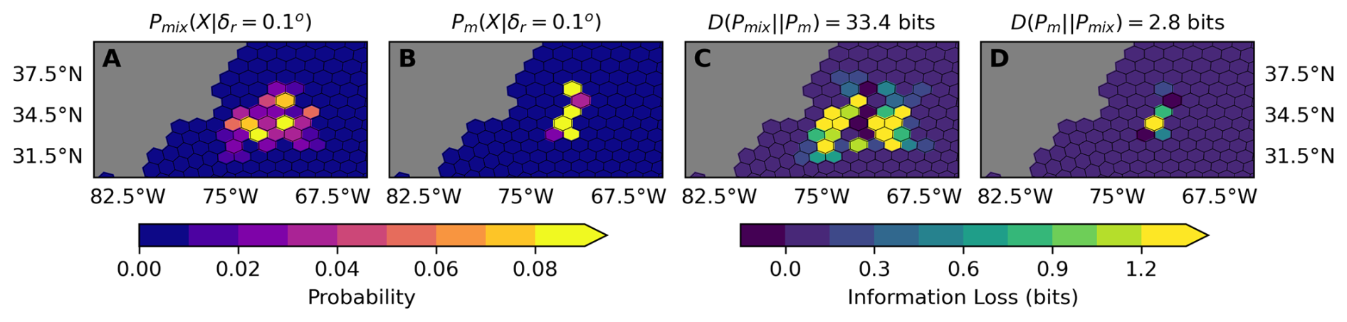
Figure 3 Comparison of probability distributions and their relative entropy. (A) Mixture distribution $P_{\text{mix}}\left(X\right|{\mathit{\delta }}_{\mathrm{r}}=\mathrm{0.1}\mathit{°}$) at 15 d after release, representing the full probabilistic model. (B) Single-member distribution $P_m\left(X\right|{\mathit{\delta }}_{\mathrm{r}}=\mathrm{0.1}\mathit{°}$) at 15 d after release, representing the reduced-order approximate model. (C) Information loss map showing the contribution of each grid cell to the total relative entropy $D\left(P_{\text{mix}}\right|\left|P_m\right)$ when approximating the mixture distribution with the single-member distribution. (D) Information loss map showing the contribution of each grid cell to the total relative entropy $D\left(P_m\right|\left|P_{\text{mix}}\right)$ when approximating the single-member distribution with the mixture distribution. Gray hexagons represent land. Color scales show probability values (A, B) and information loss in bits (C, D). The zero-bit value falls within the second color bin from the left in the information loss color scale.

3 Results

3.1 Connectivity

This section compares mixture simulations (containing the full ensemble variability) and single-member distributions for particles crossing the 40° W line. Throughout this analysis, we use the mixture distribution with δ_r=0.1° as our reference, as it represents the closest approximation to a point release, while still being controlled by the variability in ocean velocities from the full ensemble variability. This allows us to consistently evaluate how increasing spatial or temporal variability in single-member simulations compares to this baseline case. We employed empirical cumulative distribution functions (ECDFs) to assess the likelihood of single-member distributions matching the average particle counts in mixture distributions. Figure 4 shows the ECDFs for the number of particles crossing 40° W and the median particle age at which they cross that longitude. Figure 4A and B compare spatially varying releases and the releases with added diffusion, whereas Fig. 4C and D compare temporally varying release simulations. In all panels, the ECDF curves represent the single-member distributions, and the vertically shaded lines show the 99 % confidence interval of their corresponding mixture distributions. The mixture distributions are depicted as vertically shaded lines to enhance the readability of the plots since they are well-defined Gaussian distributions. The plots showing kernel density estimate (KDE) distributions of the single-member and of the mixture distributions can be found in Figs. B3 and B4, in the Appendix B.

Figure 4A shows greater variance in single-member distributions than mixture distributions, with values ranging from 1000 to 5100 particles. This increased variability occurs because single-member distributions reflect the specific ocean conditions of individual ensemble members, while mixture distributions average out these individual variations across multiple members, resulting in more stable statistics. On average, more particles cross the 40° W line for simulations with larger release clouds δ_r in the single-member distributions. The same relation between δ_r and the number of particles crossing is observed in the mixture distributions. The ECDF provides insights into the probability of single-member simulations not capturing the mixture distribution averages. For instance, in single-member simulations with a release radius of δ_r=0.1°, there is a 0.64 probability of having fewer particles crossing the 40° W line than the average of the mixture distribution with δ_r=0.1°, and consequently, a 0.36 probability of overestimation. The probability of underestimation decreases to 0.34 (with 0.66 probability of overestimation) for δ_r=1.0° and to 0.10 (with 0.90 probability of overestimation) for δ_r=2.0°, taking the same mixture distribution (δ_r=0.1°) as reference.

Figure 4C shows the ECDFs for temporally varying releases. The distributions for the single-member simulations with 4, 12, and 20-week releases are similar but show more variance than the mixture distributions represented by the shaded lines. Mixture distributions for 4- and 12-week releases have comparable average particle counts, while 20-week releases show slightly lower averages. For single-member simulations, the probability of having fewer particles than the mixture distribution average (δ_r=0.1°) is 0.56 (with 0.44 probability of overestimation) for 4-week releases, 0.50 (with 0.50 probability of overestimation) for 12-week releases, and 0.66 (with 0.34 probability of overestimation) for 20-week release periods.

Figure 4E shows that the single-member simulations with low diffusion (K_h=10 m² s⁻¹) have a distribution similar to the single-member simulations with δ_r=0.1°, for which there is a 0.70 probability of having fewer particles crossing the 40° W line than the mixture δ_r=0.1° distribution. The simulations with high diffusion have a distribution where there is a zero chance that fewer particles cross the 40° W line than in the mixture δ_r=0.1° distribution, which means that connectivity is very likely to be overestimated in this simulation with high diffusion.

Figure 4B shows the ECDFs for the median particle age of particles crossing 40° W in spatially varying release simulations. The single-member distributions (ECDF curves) show a clear separation based on the release cloud size (δ_r). Particles from smaller release clouds (δ_r=0.1°) tend to have longer median drift times, while those from larger release clouds (δ_r=2.0°) have shorter median drift times. This trend is also reflected in the mixture distributions' 99 % confidence interval (shaded lines). While the single-member simulations show a greater spread in median drift times compared to the mixture distributions, they maintain the same general pattern of decreasing drift times with increasing release cloud size. However, the wider spread in single-member distributions indicates that individual simulations may not consistently reproduce the more stable statistics captured by the mixture distributions.

Figure 4D shows the ECDFs for particle age in temporally varying release simulations. The distributions for different release durations (4, 12, and 20 weeks) are more closely aligned than the spatial variations in panel (B). However, longer release periods (20 weeks) tend to show slightly shorter median drift times. While single-member distributions still exhibit greater variability than the mixture distributions, this variability is less pronounced than in the spatially varying simulations. This suggests that temporal release variations may provide more consistent reproducibility of mixture statistics compared to spatial variations, although this varies in individual simulation results.

Figure 4F shows that the ECDF for single-member simulations with low diffusion (K_h=10 m² s⁻¹) shows similar median particle age distribution to the single-member simulations with δ_r=0.1°. The particles in the simulations with high diffusion (K_h=1000 m² s⁻¹) have both a much lower average age and a much lower spread in their age when they cross the 40° W line than in any of the other strategies.

In summary, our connectivity analysis reveals that single-member simulations tend to either significantly under- or overestimate particle transport across 40° W, with the bias depending on the release strategy. For spatial variations, larger release clouds (δ_r=2.0°) show a strong tendency to overestimate connectivity (90 % probability), while smaller release clouds (δ_r=0.1°) are more likely to underestimate it (64 % probability). Temporal variations show more balanced probabilities of under- and overestimation, particularly for 12-week releases (50 %–50 % probability), and generally exhibit less pronounced variability in particle ages compared to spatial variations. Adding a low amount of diffusion (K_h=10 m² s⁻¹) is likely to underestimate particle transport (70 % probability), while high diffusion (K_h=1000 m² s⁻¹) is certain to overestimate particle transport.

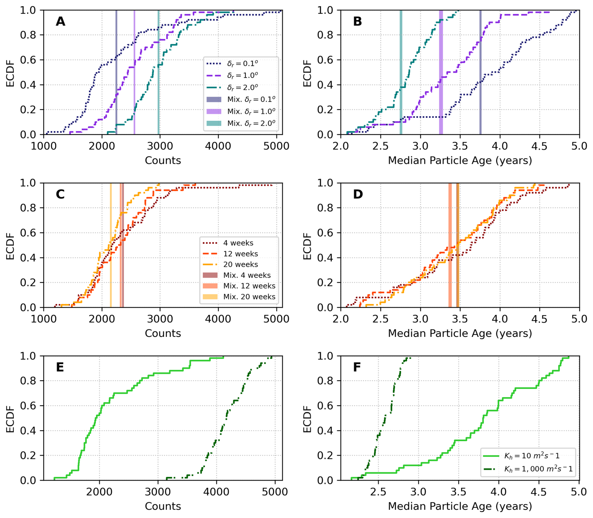
Figure 4 Connectivity analysis between the Gulf Stream at Cape Hatteras and the line at 40° W in the North Atlantic. The plots compare single-member ECDFs (lines) with mixture distribution average plus/minus 99 % confidence values (shaded vertical lines). (A) ECDFs of the number of particles crossing the line for spatially varying simulations (B) ECDFs of the median particle age distributions for spatially varying releases and simulations with diffusion. (C) ECDFs of the number of particles from temporally varying simulations. (D) ECDFs of the median particle age distributions for temporally varying simulations. (E) ECDFs of the number of particles from simulations with diffusion. (F) ECDFs of the median particle age distributions for simulations with diffusion.

3.2 Two-dimensional probability distributions

The first step to calculate the marginal and relative entropy is to bin the particle trajectories into the two-dimensional probability distributions in the hexagonal grid. We computed the two-dimensional probability distributions for all the single-member and mixture simulations, for the different strategies to generate variability in the trajectories. As an illustration, Fig. 5 shows the two-dimensional probability distributions for the reference mixture δ_r=0.1° distribution (subset 43) and the single ensemble member distributions, with different release strategies (ensemble member 22). The three columns of subplots show the distributions at particle ages of 10, 100, and 1000 d, and the different rows show the different strategies to generate variability. We observe that the reference mixture δ_r=0.1° distribution, showcasing the full ensemble variability, spreads evenly from the release location (shown as a blue dot). We also appreciate how 20-week and δ_r=2.0° single-member distributions resemble the mixture distribution in the area covered by the bins, but the shape of the distributions still remains different. However, the distributions from the single-member simulations with δ_r=0.1° and low diffusion (K_h=10 m² s⁻¹) clearly cover fewer bins at the three particle ages shown, despite having the same number of particles as the other distributions. The distribution from the simulations with high diffusion (K_h=1000 m² s⁻¹) covers a similar range of bins to the δ_r=2.0° single-member distribution for 10 d; it covers many more bins for 100 d and then looks fairly similar to the other distributions for 1000 d. Figures B5 and B6, in the Appendix B, show similar figures but with other single members and mixture subsets. In general, two-dimensional distributions can best be described and compared with statistical tools. Thus, we computed the marginal entropy and relative entropy of these distributions, at different particle ages, to characterize and compare the dispersion patterns of the different single-member strategies to that of the reference mixture.

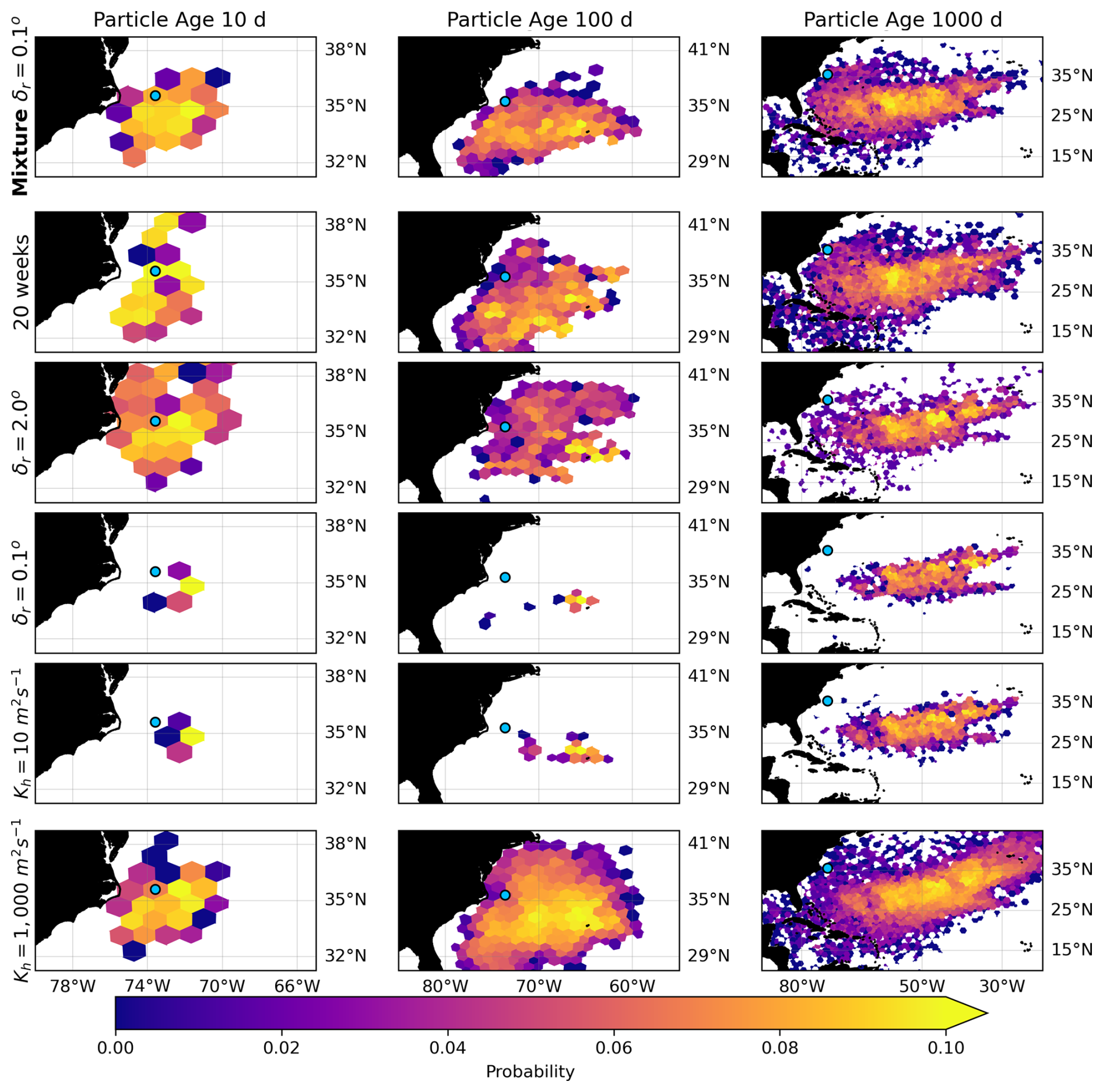
Figure 5 Probability distributions of particle locations at different ages (10, 100, and 1000 d; columns) across varying release strategies (rows). The top row shows the probability of the mixture δ_r=0.1° distribution (mixture subset 43 of the bootstrapping). The second, third, fourth, and fifth rows show the single-member distributions (member 22), with 20-week, δ_r=2.0°, δ_r=0.1°, and with diffusion K_h=10 m² s⁻¹ and K_h=1000 m² s⁻¹. The blue circles mark the particle's release location, omitted for plots of particle age of 10 d. Bins with probability zero were removed to facilitate visualizing the area of dispersal of the particles.

3.3 Marginal and relative entropy

We calculated the marginal entropy (Eq. 6) for every single-member and corresponding mixture distribution to assess the variability and determine which release strategies can represent the variability of the full ensemble. In total, we computed the marginal entropy functions for all eight sets of single-member distributions (three spatial varying, three temporal varying, and two diffusive). We also computed the marginal entropy for six sets of mixture distributions, excluding the mixture distribution from simulations with diffusion. Each release strategy and mixture set had 50 distributions; therefore, we calculated the average and the standard deviation of the marginal entropy functions, resulting in one average entropy curve as a function of particle age per set. Figure 6A illustrates the average entropy curves for spatially varying release distributions, while Fig. 6B shows those for temporally varying release distributions and Fig. 6C shows those for distributions with diffusion. Detailed entropy curves for each single-member and mixture simulation are provided in Figs. B7 and B8 in the Appendix B.

Figure 6A shows the average marginal entropy as a function of particle age for various spatial release strategies, comparing single-member probability distributions (P_m) with mixture distributions (P_mix) using different spatial release intervals (δ_r). Three single-member curves are shown: δ_r=0.1° (blue dotted line), δ_r=1.0° (purple dashed line), and δ_r=2.0° (green dash-dot line). Two mixture distribution curves are presented: δ_r=0.1° (solid black line) and δ_r=2.0° (black dash-dot line). Shaded areas around the single-member curves represent the standard deviation, illustrating the spread of entropy values across the ensemble. There is no shaded area around the mixture entropy curves because their standard deviation was of the order of magnitude 10⁻² bits. The logarithmic scale on the x axis emphasizes the rapid changes in entropy during the early stages of particle dispersion. All curves show a logarithmic increasing trend in entropy with particle age, indicating growing dispersion over time. The single-member distributions with larger δ_r values (1.0 and 2.0°) initially overestimate the entropy compared to the mixture distribution with δ_r=0.1°, particularly in the first 10 d. After this period, only the single-member distribution with δ_r=2.0° adequately represents the variability of the mixture with δ_r=0.1°.

Figure 6B shows the average entropy as a function of time for the temporal varying release strategies and their corresponding mixture distributions, comparing single-member probability distributions P_m for different release periods against mixture distributions (P_mix). The single-member distributions are shown for release periods of 4, 12, and 20 weeks. These curves show a general trend of entropy increasing logarithmically over time, with longer release periods resulting in higher entropy values. Three mixture distributions are plotted: mixture subsampled from 4-week release, mixture subsampled from 20-week release, and the reference mixture from δ_r=0.1°. We compared temporal and spatial mixture distributions to understand how different release strategies contribute to the total ensemble variability. As one would expect, these mixture distributions consistently show higher entropy values than single-member distributions, indicating that P_m captures less variability than the mixture distributions. The 20-week single-member average entropy closely follow the reference mixture δ_r=0.1° average entropy, often overlapping or slightly exceeding it. Among the single-member curves, the 20-week release generally shows the highest average entropy, followed by 12 and 4 weeks in descending order. However, these differences become less pronounced as time increases.

Figure 6C shows the average entropy as a function of time for the simulations with diffusion. The simulations with the low diffusion (K_h=10 m² s⁻¹) show very low entropy for the first 10 d, somewhat similar to the single-member curve of δ_r=0.1° in Fig. 6A. The simulations with the high diffusion (K_h=1000 m² s⁻¹), on the other hand, track the δ_r=0.1° mixture distribution (solid black line), with a slight underestimation in the first 20 d and a slight overestimation between 20 and 1000 d.

Comparing spatial and temporal strategies in Fig. 6A and B supports setting the mixture distribution with δ_r=0.1° as our reference standard, as it shows the minimum average entropy among all mixture strategies but still captures the full ensemble variability. The 20-week single-member average entropy curve most closely approximates the reference mixture δ_r=0.1° entropy, while the single-member spatial releases show more variable performance. Both the δ_r=2.0° and the 20-week mixture distributions exhibit the highest average entropy values, demonstrating how combining either spatial or temporal release strategies with the ensemble variability increases the total dispersion variability. This reinforces our choice of the more point-like δ_r=0.1° mixture as our reference for evaluating single-member approximations. For clarity, we omitted the intermediate mixture curves (δ_r=1.0° and 12-week), as their entropy values consistently fall between those of the δ_r=0.1° and δ_r=2.0° and 4 and 20 weeks, respectively.

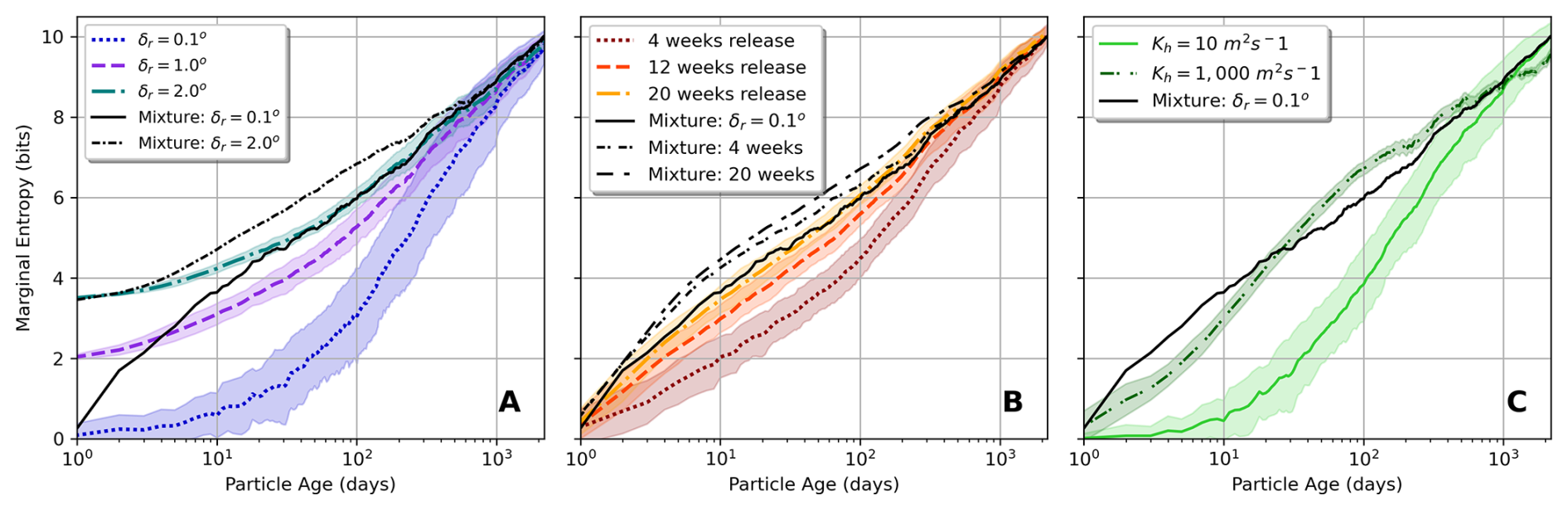
Figure 6 Average marginal entropy as a function of particle age of single-member distributions (colored lines) and mixture distributions (black lines). The average marginal entropy for the single-member simulations with diffusion K_h is shown as black triangle curve. The shaded areas represent the standard deviation. The particle age is on a logarithmic scale. (A) Comparison of the single-member and mixture distributions with spatially varying release. (B) Comparison of the single-member and mixture distributions with temporally varying release. (C) Comparison of the single-member distributions with diffusion. In all panels, we added the entropy curve of the mixture δ_r=0.1° as a reference.

We computed the relative entropy as a function of particle age by comparing single-member distributions with mixture distributions, to understand how similar the single-member distributions are to the mixture distributions, bin by bin. For this, we computed the relative entropy of a single-member distribution P_m(X,t) compared to a mixture distribution P_mix(X,t), using Eq. (10), across all their particle ages. Therefore, we calculated 50²=2500 relative entropy curve as a function of particle age curves when comparing two sets of distributions: that is, one set for single-member simulations and one set of mixture simulations. From the 2500 relative entropy functions, we computed the average and the standard deviation of the relative entropy as a function of particle age. We computed the average relative entropy for the combination of the seven sets of single-member distributions (${\mathit{\delta }}_{\mathrm{r}}\in \mathit{\{}\mathrm{0.1}\mathit{°},\mathrm{1.0}\mathit{°},\mathrm{2.0}\mathit{°}\mathit{\}}$, 4, 12, and 20 weeks, and K_h=10 m² s⁻¹ and K_h=1000 m² s⁻¹), with the six sets of mixture distributions (excluding diffusion), ending up with 48 average relative entropy curve as a function of particle age.

Figure 7 shows the average relative entropy as a function of particle age, divided into four panels (A–D), each using a different mixture distribution as a reference (P_mix). In these plots, low values of the relative entropy indicate good agreement to the reference case, as relative entropy is a measure of the mismatch between each of the distributions shown and the reference distribution (technically: the cost of assuming that each of the distributions shown is the reference distribution). We omitted the plots where the mixture δ_r=1.0° and mixture 12-week strategy was used a reference, since their entropy lies between their corresponding extreme strategies, that is ${\mathit{\delta }}_{\mathrm{r}}\in \mathit{\{}\mathrm{0.1}\mathit{°},\mathrm{2.0}\mathit{°}\mathit{\}}$ and 4- and 20-week releases. In all panels, the solid and dotted lines represent the average relative entropy for each strategy, while the shaded bands around these lines indicate their corresponding standard deviation. The standard deviation measures the variability in relative entropy, revealing the extreme cases where single-member distributions poorly represent the reference mixture distributions.

Figure 7A uses the reference mixture distribution with δ_r=0.1° as the reference (P_mix). On average, the single-member distribution with δ_r=2.0° (green dotted line) most closely approximates the reference mixture, having the lowest mean relative entropy across most of the time range. The 20-week release strategy (yellow dashed line) and K_h=1000 m² s⁻¹ (purple dashed line) perform similarly well. However, δ_r=0.1° (blue dash-dot line), the 4-week release (red dotted line), and K_h=10 m² s⁻¹ (black line) have higher average relative entropy, showing that their two-dimensional distributions under-represent P_mix. Regarding their standard deviation bands, we see that δ_r=2.0° has almost zero standard deviation on the first 10 d after release. This is due to the larger area being covered by particles at the release compared to the area covered by the P_mix. The opposite case is observed with δ_r=0.1° and K_h=10 m² s⁻¹ standard deviations, which indicate a more likely greater lack of information compared to the reference distribution P_mix.

Figure 7B, with the mixture distribution with δ_r=2.0° as reference P_mix, shows that the single-member δ_r=2.0° strategy most closely matches P_mix on average. The 20-week release strategy and K_h=1000 m² s⁻¹ also perform well, especially for higher particle ages. The substantial standard deviations for all strategies, particularly pronounced for δ_r=0.1°, the 4-week strategy, and K_h=10 m² s⁻¹, highlight the potential for large lack of information in representing P_mix at all particle ages. Figure 7C and D use the 4- and 20-week mixture distributions as references, respectively. In both cases, 20-week and δ_r=2.0° single-member temporal release strategies, and the K_h=10 m² s⁻¹ show the lowest mean relative entropy. The wide standard deviation bands, particularly noticeable for δ_r=0.1° and K_h=10 m² s⁻¹, underscore the high variability in how well these strategies capture the reference mixture's characteristics.

Across all panels of Fig. 7, relative entropy peaks between 10 and 100 d of particle age, with the largest standard deviations also occurring in this range. Notably, standard deviations for temporal (20-week) and spatial (δ_r=2.0°) strategies peak at different times: the 20-week release shows maximum variability at earlier particle ages (before 10 d), while the δ_r=2.0° release peaks later (before 100 d). This suggests that these single-member strategies are most likely to significantly diverge from the mixture distributions around these particle ages.

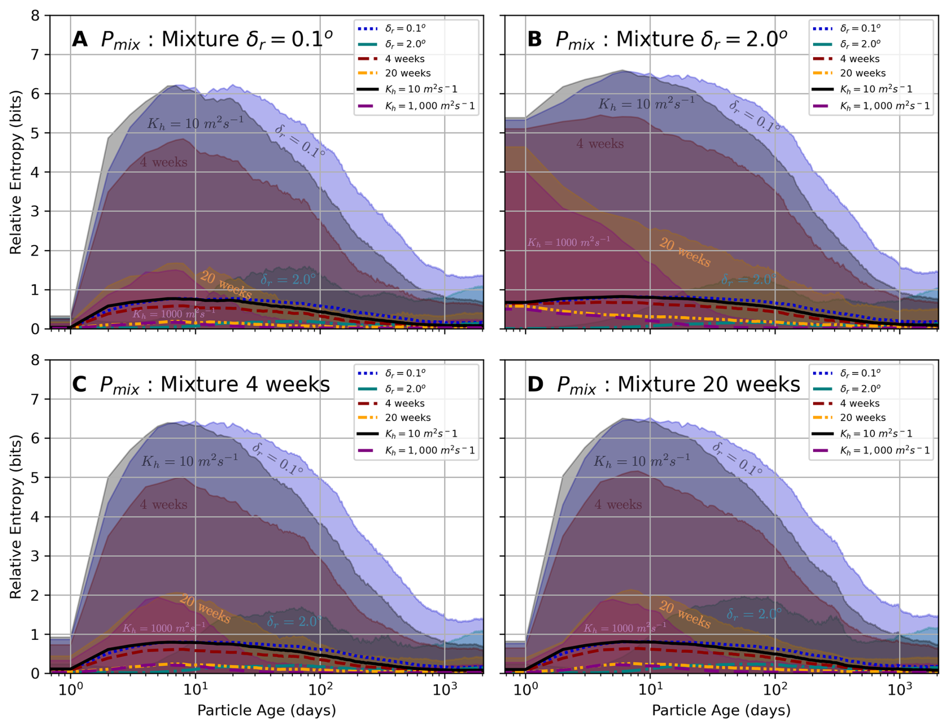
Figure 7 Relative entropy as a function of particle age for different single-member distributions compared to mixture distributions. The subplots (A)–(D) show comparisons using different reference mixture distributions (P_mix): (A) δ_r=0.1°, (B) δ_r=2.0°, (C) 4-week release, and (D) 20-week release. Dotted and solid lines represent the average relative entropy for each release strategy, while shaded areas indicate their corresponding standard deviation. The x axis shows particle age in days (log scale), and the y axis shows relative entropy in bits. Different colors represent various single-member strategies: δ_r=0.1° (blue), δ_r=2.0° (green), 4-week release (red), 20-week release (orange), K_h=10 m² s⁻¹ (black), and K_h=1000 m² s⁻¹ (purple).

From the average entropy curves shown in Fig. 7, we took the average over the 6 years the particles were drifting after release. We compiled these values for the 20 comparisons between mixture and single-member sets, with different release strategies in Fig. 8. This figure presents a heatmap of the time-averaged relative entropy values for various combinations of single-member and mixture distributions. The rows represent single-member distributions, while the columns represent mixture distributions. The color scale ranges from dark green (lowest relative entropy) to light green (highest relative entropy), with numerical values provided in each cell. Notably, the K_h=1000 m² s⁻¹ (last row) and 20-week single-member distribution (fourth row) consistently shows the lowest relative entropy across all mixture distributions, indicating both strategies best represent the ensemble variability. Conversely, the δ_r=0.1° single-member distribution exhibits the highest relative entropy values, followed by K_h=10 m² s⁻¹, suggesting that they are the least effective at capturing the characteristics of the mixture distributions.

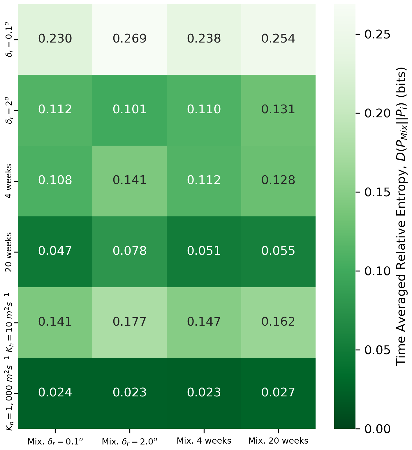
Figure 8 Time-averaged relative entropy (in bits) between single-member and mixture distributions for different release strategies. Rows represent single-member distributions, and the columns represent mixture distributions. Color intensity indicates the magnitude of relative entropy, with dark green representing lower values (better agreement) and light green representing higher values (poorer agreement). Numerical values in each cell show the precise time-averaged relative entropy.

4 Discussion and conclusions

In this study, we investigated how to generate ensemble-like variability within single-member Lagrangian simulations by implementing varying spatial and temporal release strategies, as well as by adding diffusion, in the Gulf Stream region near Cape Hatteras. The surface connectivity between the Gulf Stream and the region past 40° W revealed significant differences in the number of particles crossing between different release strategies in the single-member distributions. The ECDFs in Fig. 4 showed that, for spatially varying releases, the larger the initial particle cloud, the more particles cross the 40° W. Regarding the temporal distributions, we did not see significant variations in the number of particles crossing 40° W; the distributions for the number of particles and the median times were similar between the three temporal release strategies. The low-diffusion K_h distribution was very similar to the spatial δ=0.1° distribution, with fewer particles crossing 40° W than other strategies, while the high-diffusion K_h distribution resulted in complete connectivity on much shorter timescales than any other strategy. Moreover, the normal distribution observed in the mixture distributions can be attributed to the central limit theorem. This fundamental principle in probability theory states that when independent random samples are drawn from a population with a finite variance, the distribution of their means will approximate a normal distribution as the sample size increases. In our case, the bootstrapping method used to construct the mixture distributions effectively simulates this sampling process, resulting in the observed normal distributions.

Regarding representing the full ensemble variability with single-member simulations in the connectivity analysis, we see that particles are more consistent in crossing the 40° W meridian in the mixture distributions. Therefore, when comparing mixture distributions with single-member distributions, we counted the percentage of single-member simulations with fewer particle crossings than the reference mixture distribution with δ_r=0.1°. In this analysis, we see that performing a one-time spatial release with a radius of δ_r=2.0° better represents the particle crossings in the mixture distributions than the other strategies. From all the release strategies, single-member simulations with δ_r=2.0° release cloud had the lowest likelihood of having fewer particles crossing than the reference mixture simulation with δ_r=0.1°. This might be because a large initial cloud of particles releases more particles outside the Gulf Stream, creating a wider variety of trajectories that cross 40° W. In the case of the temporal releases, the single member with 20-week release simulation had fewer particles crossing 40° W than the mixture with δ_r=0.1°, with a 66 % likelihood of having fewer particles. This likelihood is 10 % higher than 4- and 12-week single-member distributions, suggesting that the seasonability may be playing a role in the transport of particles to the eastern side of the domain. The connectivity with the eastern region of the domain might be stronger during winter, corresponding to the release of particles in the 4-week period (from 2 to 30 of January) and 12-week period (from 2 January to 27 March). Meanwhile, the 20-week release, from 2 January to 22 May, had a portion of its particles released during spring.

The marginal entropy analysis, shown in Fig. 6, provided insights into how well different release strategies represent the full ensemble variability. In general, we see how the marginal entropy increased with time for all strategies considered, some at slower rates than others. We attributed this to the percentage of particles released under the local decorrelation length scales and timescales for the different strategies. For instance, spatial releases with radius δ_r=0.1° and temporal releases of 4 weeks, which exhibited the lowest marginal entropy, had all their particles released within their respective decorrelation scales. As the radius or release period was increased, there were more particles with decorrelated initial velocities, resulting in higher entropy in the two-dimensional distributions.

It is important to highlight that the marginal entropy of the mixture distributions consistently exceeds that of corresponding single-member distributions, demonstrating that ensemble simulations under identical release conditions inherently generate greater trajectory variability than single-member simulations. By maintaining equal particle counts between mixture and single-member simulations, we ensured that the higher entropy in mixture distributions reflects genuine ensemble dynamics rather than statistical artifacts. The higher marginal entropy in mixture distributions may also be attributed to the temporal context of our study: we advected particles ∼18 years after the initialization of the NATL025-CJMCYC3 ensemble (which was perturbed during 1993). At the release date of the particles (2010), the perturbations had sufficient time to adapt and decorrelate the velocity fields of the members, which suggests that ensemble Lagrangian dispersion arises not only from mesoscale chaos but also from low-frequency, large-scale intrinsic fluctuations.

Based on the marginal entropy curves from Fig. 6, we selected the mixture simulations with δ_r=0.1° as reference for comparing the different release strategies because they contain the full ensemble variability with least noise added by the initial perturbation to their initial conditions. Comparing the spatial releases against this reference (Fig. 6A) revealed significant limitations. The larger release areas (δ_r=1.0° and δ_r=2.0°) initially overestimate variability during the first 10 d, as particles start from a wider area than the reference's mixture with δ_r=0.1° radius. While δ_r=2.0° simulations eventually match the reference entropy after 30–40 d, δ_r=1.0° simulations underestimate it until about 1000 d after release.

The simulations with low diffusion (K_h=10 m² s⁻¹) show marginal entropy similar to spatial releases with δ_r=0.1° but fail to reproduce the full ensemble variability until approximately 1000 d after release, as seen in Fig. 6. The simulations with high diffusion (K_h=1000 m² s⁻¹), on the other hand, lead to very similar entropy statistics as the mixture models (Fig. 8), although they fail to capture the connectivity and transport time patterns. These added diffusion simulations used a stochastic differential equation approach with Brownian motion terms, following established methods in Lagrangian oceanography (Griffa, 1996). Our results demonstrate that such an approach could reproduce some of the full ensemble entropy but at the expense of overestimating the connectivity. Furthermore, Brownian diffusion can also move particles across permanent fronts or (if not treated carefully), even across landmasses such as the Panama Isthmus (McAdam and Van Sebille, 2018).

The underperformance of the low diffusion strategy likely reflects that it represents primarily small-scale turbulent mixing processes, and the diffusion cannot create noticeable variability in trajectories, specially for particle ages <100 d, missing the larger-scale flow uncertainties and mesoscale variability captured through other strategies. In contrast, temporal release strategies (Fig. 6B) show better performance, particularly the 12- and 20-week releases. The 20-week release strategy consistently matches the reference mixture's marginal entropy (mixture δ_r=0.1°) across all temporal scales, demonstrating that continuous particle releases over time can effectively reproduce the variability captured by ensemble simulations. This suggests that temporally varying the initial conditions is more effective at generating ensemble variability than adding diffusion and also is more consistent throughout particle ages than varying spatially the extent of the release area.

As we explained in Sect. 2.4.4, two distributions that have the same entropy do not necessarily exhibit the same distributions since two different probability distributions can have equivalent marginal entropies. As a complementary analysis, we computed the relative entropy to measure the agreement between two distributions, which measures the lack of information when representing the full ensemble with a single-member simulation. We applied the relative entropy analysis to compare all release strategies against the mixture distribution δ_r=0.1°. The averaged results and their variability, shown in Fig. 7, further support the findings from the marginal entropy assessment. The 20-week and K_h=1000 m² s⁻¹ release generally showed consistently low average relative entropy with respect to the reference mixture distribution, indicating this release strategy most effectively captured the particle distributions over time, by generating two-dimensional distributions that resembled the most to the ones of the mixture distribution containing the full ensemble variability. Contrary to that, the δ_r=0.1°, 4-week, and K_h=10 m² s⁻¹ strategies showed the largest values in average relative entropy, with large standard deviations in particle ages below 100 d. This shows that these strategies have particular difficulty to generate variability in the trajectories similar to a full ensemble.

Comparing the 6-year time-averaged relative entropy, shown in Fig. 8, showed how the 20-week release strategy and the K_h=1000 m² s⁻¹ simulations have least uncertainty and how they represent the best full ensemble variability across different reference mixtures. The δ_r=2.0° and a 4-week release strategy showed higher uncertainties compared to a 20-week release. Lastly, K_h=10 m² s⁻¹ and δ_r=0.1° had the highest time-average relative entropies. This further supports the idea that performing long continuous releases is the best release strategy to generate variability in particle trajectories similar to a full ensemble simulation.

In single-member simulations, we demonstrated that releasing particles at slightly different locations or times can match the variability in the behavior of particles released at a specific time and location from an ensemble of simulations. An interpretation of this may be that an ensemble of Lagrangian simulations has an ergodic flavor in which statistical homogeneity exists between an ensemble of simulations and single-member simulations (Shannon, 1948). However, this does not constitute proof of the system's ergodicity.

While our study provides valuable insights into generating ensemble-like variability in single-member simulations, several limitations should be acknowledged. Our analysis focused solely on the Gulf Stream region near Cape Hatteras, and the effectiveness of these release strategies may vary in other oceanic regions with different dynamics. Additionally, while our particles were advected in three-dimensional flows, we only considered surface particle releases, which may not fully represent the three-dimensional transport processes occurring throughout the water column. Our results are based on the NATL025-CJMCYC3 model configuration, and the effectiveness of these strategies may be resolution-dependent, as higher-resolution models resolve smaller-scale processes that could introduce additional variability in transport pathways. We performed simulations for only one release period, on 2 January 2010, because that allowed us the longest particle advection time. We acknowledge, however, that the results presented here may depend on the chosen release time. Furthermore, our study was limited to forward-in-time simulations, whereas backward-in-time tracking could provide complementary information about generating ensemble variability in single-member simulations in studies concerning source regions and transport pathways. Future work should explore the potential of the framework and methods provided in this study across different oceanic regions, depths, and temporal directions to establish more comprehensive guidelines for single-member Lagrangian simulations, including appropriate values for K_h in random walk diffusion parameterizations.

Ensemble simulations remain the standard for capturing the full range of variability in ocean simulations; our study provides guidance on releasing particles in single-member simulations to increase the variability of the trajectories and, in this case, better represent ensemble statistics. While data assimilative models excel at improving mean state predictions through observation integration, ensemble approaches are better suited for exploring the full range of possible outcomes and quantifying uncertainty in trajectory predictions. Generating ensemble-like variability for Lagrangian simulations advected using assimilative models could be particularly powerful: applying temporal release strategies could help capture both the improved mean state from data assimilation and the trajectory variability typical of ensemble simulations. These findings have important implications for ocean modeling and particle tracking studies, especially when computational resources limit the use of full ensemble simulations. By carefully selecting release strategies, researchers can maximize the variability of single-member simulations, potentially improving predictions of particle transport by capturing extreme events.

Appendix A: Marginal entropy as a function of number of particles and grid resolution

The calculation of the mixture probability distributions (P_mix) requires determining both the optimal number of particles to sample and the appropriate spatial resolution for binning these particles. These parameters directly affect the entropy of the resulting distributions. We investigated this relationship by varying two key parameters: the number of particles sampled per ensemble member and the hexagonal grid resolution (h).

Figure A1 shows how the entropy converges as we increase the number of particles sampled per ensemble member, plotted for three different grid resolutions ($h\in \mathit{\{}\mathrm{2},\mathrm{3},\mathrm{4}\mathit{\}}$). As expected, finer grid resolutions (larger h values) yield higher entropy values as they capture more detailed spatial information. For our chosen grid resolution of h=3, the entropy converges to approximately 8.5 bits when sampling 150 or more particles per ensemble member. Coarser resolutions (h=2) require fewer particles to converge, while finer resolutions (h=4) need more particles but capture more spatial detail. Based on this analysis, we selected h=3 and 150 particles per member as sufficient parameters for our study, balancing computational efficiency with spatial resolution.

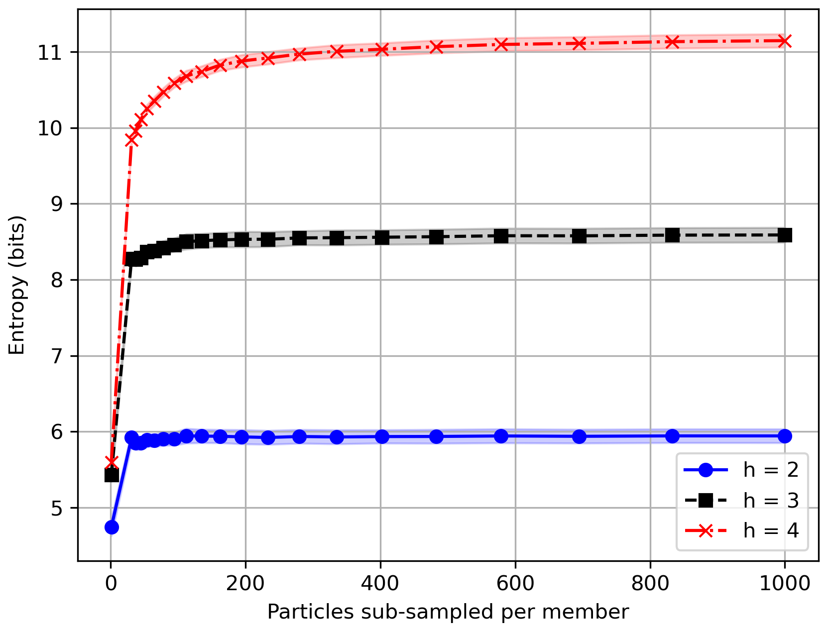
Figure A1 Marginal entropy of mixture distributions as a function of particles sampled per ensemble member, shown for three different hexagonal grid resolutions (h). Higher h values indicate finer spatial resolution, resulting in higher entropy values.

Appendix B: Additional supplementary figures

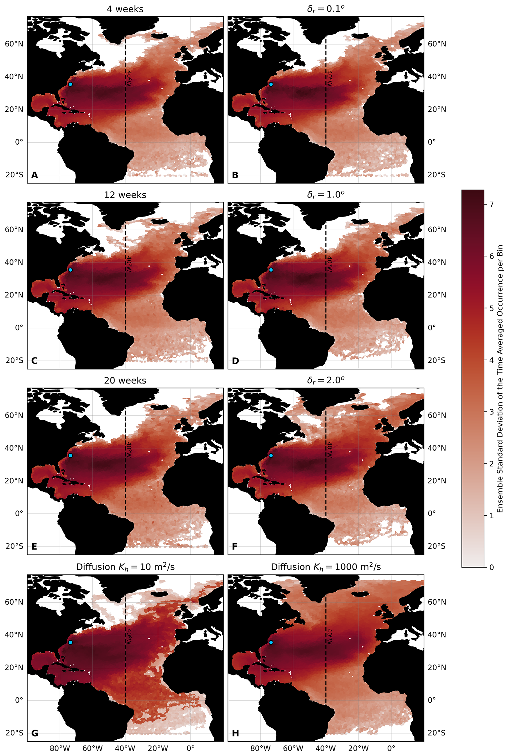
Figure B1 Ensemble standard deviation of time-averaged particle occurrence per (hexagonal) bin in the North Atlantic Ocean for single-member simulations. (A, C, E) Temporal release strategies at 4, 12, and 20 weeks. (B, D, F) Spatial release strategies with ${\mathit{\delta }}_{\mathrm{r}}\in \mathit{\{}\mathrm{0.1}\mathit{°},\mathrm{1.0}\mathit{°},\mathrm{2.0}\mathit{°}\mathit{\}}$. (G, H) Diffusion strategies with K_h=10 m² s⁻¹ and K_h=1000 m² s⁻¹. The color scale represents the ensemble standard deviation of a 6-year time-averaged occurrence per bin. The maps illustrate the variability in particle dispersal for single-member simulations. The dashed line at 40° W indicates the eastern boundary of the study area. The blue dot marks the approximate release location.

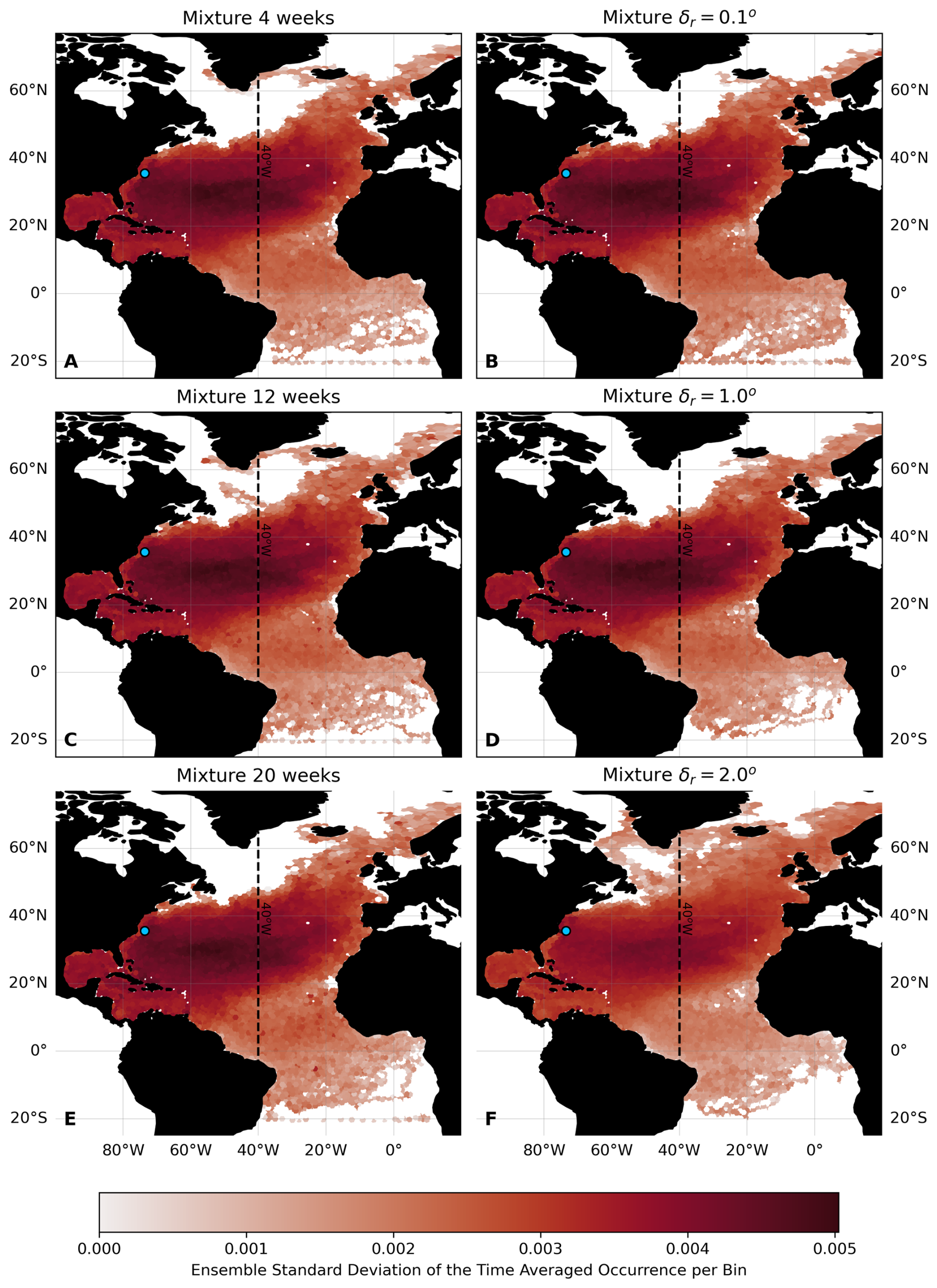
Figure B2 Ensemble standard deviation of time-averaged particle occurrence per (hexagonal) bin in the North Atlantic Ocean for mixture simulation subsets. Left column (A, C, E): mixture subsets at 4 weeks, 12 weeks, and 20 weeks. Right column (B, D, F): mixture subsets with spatial variability ${\mathit{\delta }}_{\mathrm{r}}\in \mathit{\{}\mathrm{0.1}\mathit{°},\mathrm{1.0}\mathit{°},\mathrm{2.0}\mathit{°}\mathit{\}}$. The color scale represents the ensemble standard deviation of a 6-year time-averaged occurrence per bin. The maps show the variability in particle dispersal patterns for all 50 subsets of the mixture simulations. The dashed line at 40° W indicates the eastern boundary of the study area. The blue dot marks the approximate release location.

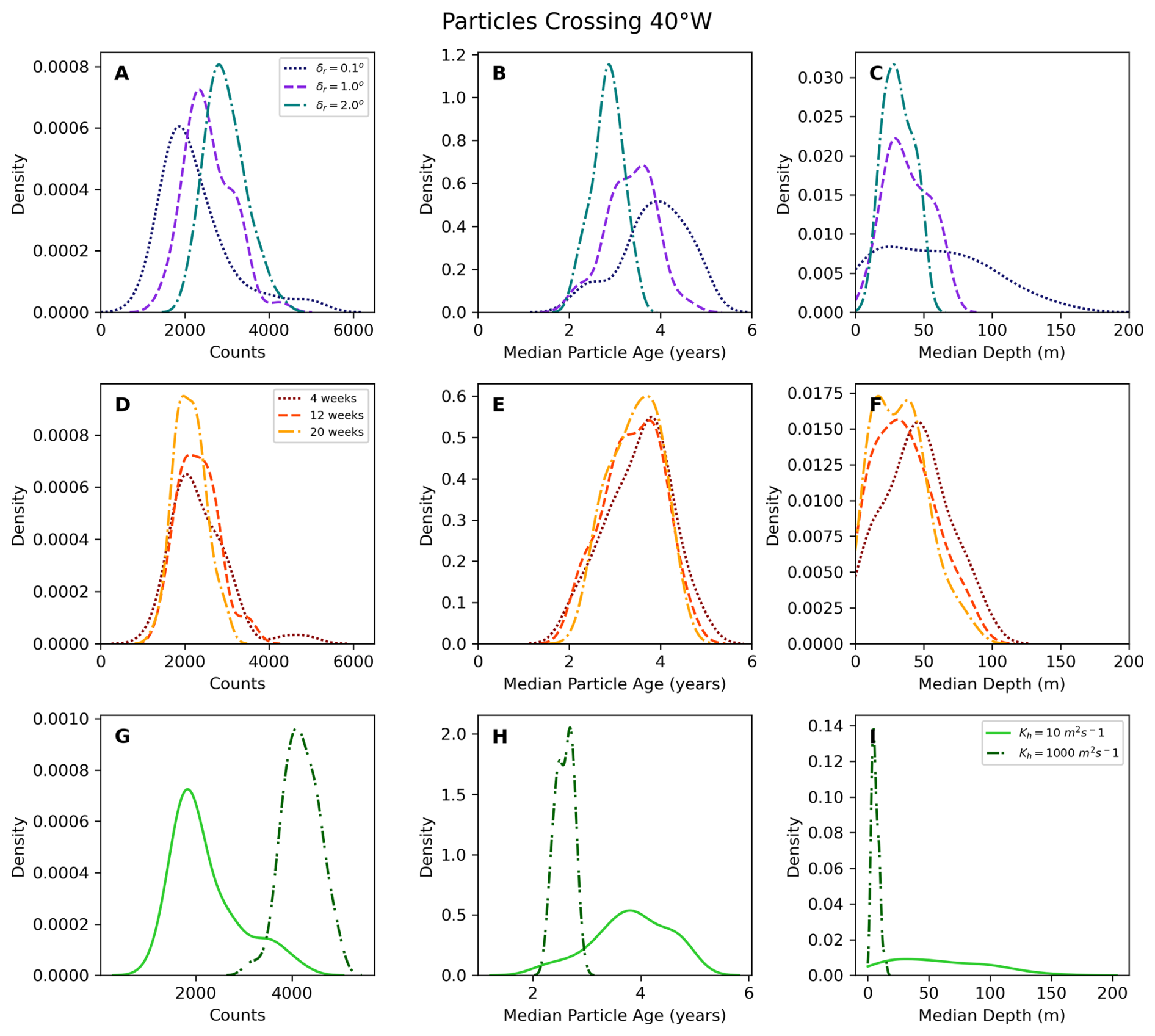
Figure B3 Kernel density estimates (KDEs) of connectivity analysis for the single-member simulations. The top row (A–C) shows distributions for spatial releases ${\mathit{\delta }}_{\mathrm{r}}\in \mathit{\{}\mathrm{0.1}\mathit{°},\mathrm{1.0}\mathit{°},\mathrm{2.0}\mathit{°}\mathit{\}}$: particle counts (A), median drift time in years (B), and median depth in meters (C). The middle row (D–F) shows the same metrics but is compared across different temporal releases of 4, 12, and 20 weeks. The bottom row (G–I) corresponds to K_h=10 m² s⁻¹ and K_h=1000 m² s⁻¹.

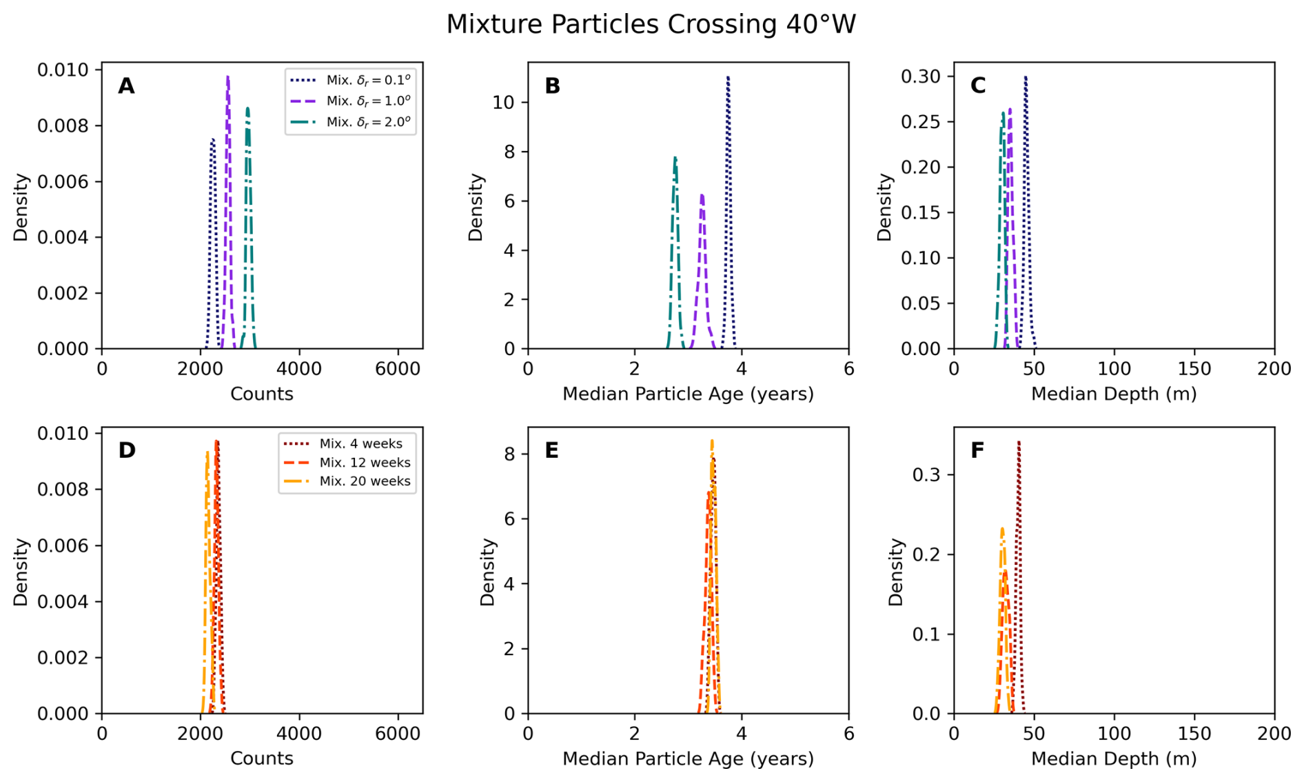
Figure B4 Kernel density estimates (KDEs) of connectivity analysis for the mixture simulations, using Scott's method with a bandwidth of 1. The top row (A–C) shows distributions for mixture spatial releases ${\mathit{\delta }}_{\mathrm{r}}\in \mathit{\{}\mathrm{0.1}\mathit{°},\mathrm{1.0}\mathit{°},\mathrm{2.0}\mathit{°}\mathit{\}}$: particle counts (A), median drift time in years (B), and median depth in meters (C). The bottom row (D–F) shows the same metrics but is compared across different mixture temporal releases of 4, 12, and 20 weeks.

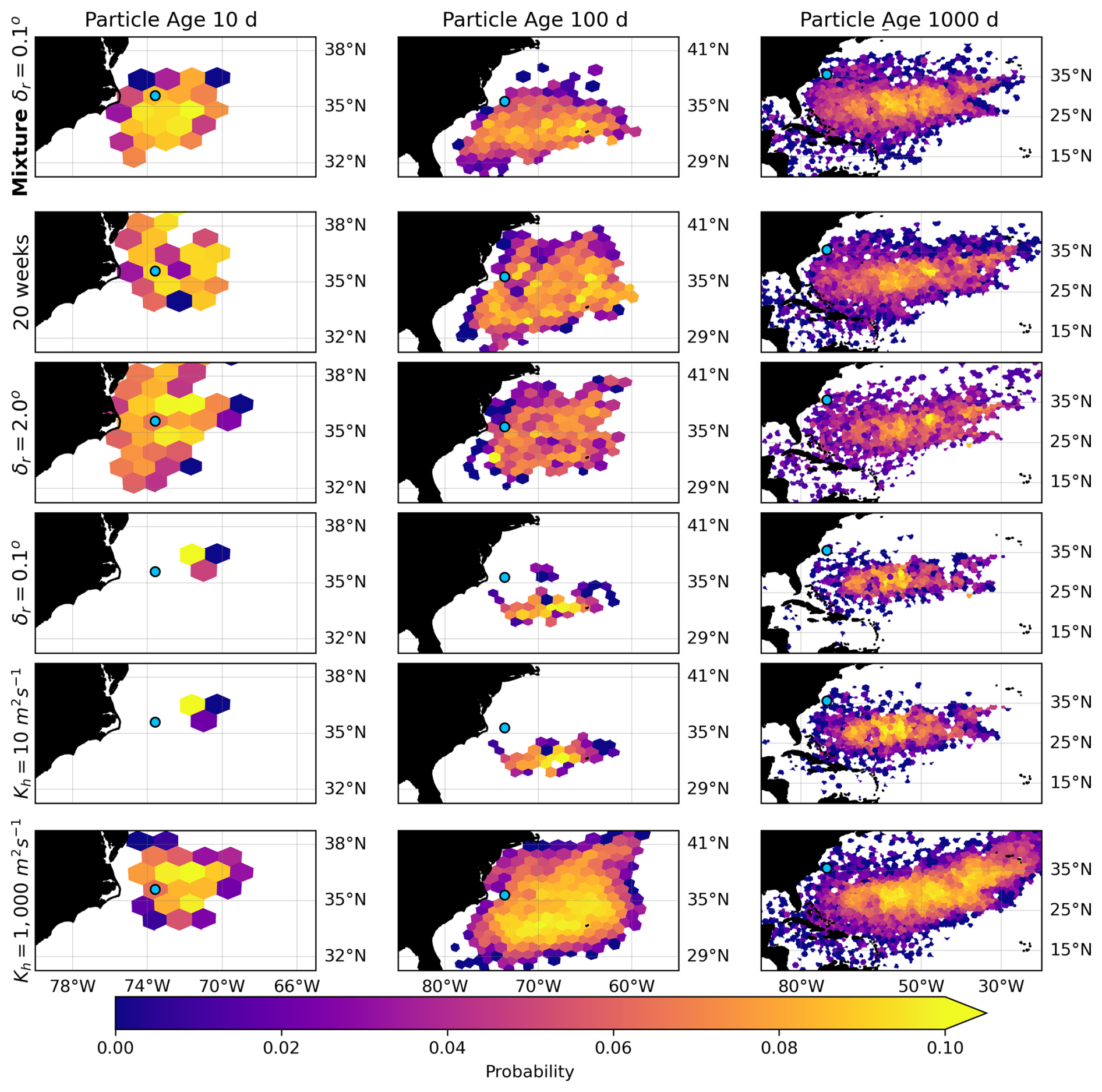
Figure B5 Probability distributions of particle locations at different ages (10, 100, and 1000 d; columns) across varying release strategies (rows). The top row shows the probability of the mixture δ_r=0.1° distribution (mixture subset 4 of the bootstrapping). From the second to the sixth row, the single-member distributions (member 17), with the following strategies: 20 weeks, δ_r=2.0°, δ_r=0.1°, K_h=10 m² s⁻¹, and K_h=1000 m² s⁻¹. The blue circles mark the particle's release location. Bins with probability zero were removed to facilitate visualizing the area of dispersal of the particles.

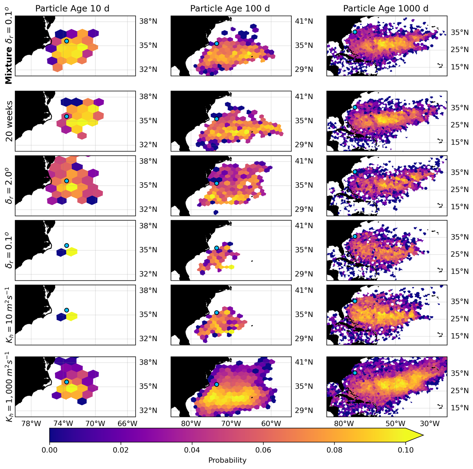
Figure B6 Probability distributions of particle locations at different ages (10, 100, and 1000 d; columns) across varying release strategies (rows). The top row shows the probability of the mixture δ_r=0.1° distribution (mixture subset 10 of the bootstrapping). From the second to the sixth row, the single-member distributions (member 46), with 20-week, δ_r=2.0°, δ_r=0.1°, K_h=10 m² s⁻¹, and K_h=1000 m² s⁻¹. The blue circles mark the particle release location. Bins with probability zero were removed to facilitate visualizing the area of dispersal of the particles.

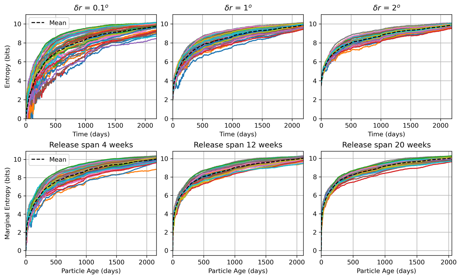
Figure B7 Marginal entropy the 50 single-member simulations performed with the different release strategies (individual panels). The lines are randomly colored, and each line represents one single-member entropy. The black dashed line is the ensemble average as a function of time.

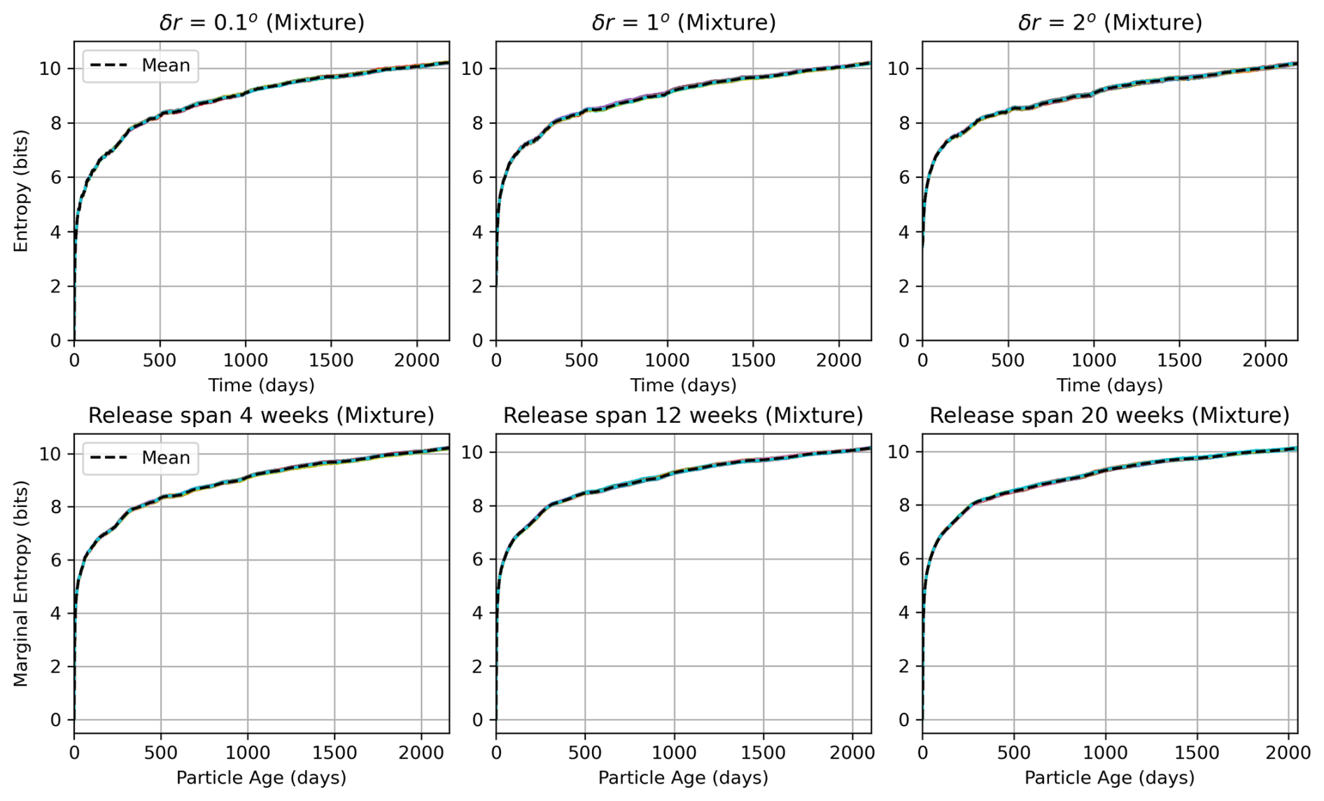
Figure B8 Marginal entropy of the 50 bootstrapping realizations or mixture distributions, subsampled from single-member simulations with different release strategies (individual panels). The color lines show the entropy of each realization, and the black dashed line is the average as a function of time.