Rate-induced transitions and noise-driven resilience in vegetation pattern dynamics

Understanding the resilience and stability of vegetation patterns under changing environmental conditions is crucial for predicting ecosystem responses to climate change. This study investigates the dynamics of vegetation patterns in response to a spatially homogeneous decrease in rainfall across the entire domain. Starting from high rainfall with a stable, homogeneous vegetated state, we applied various rates of rainfall reduction to observe system transitions. We find that rainfall decrease may cause transitions to two or three pulse states or abrupt shifts to bare soil depending on the rate of change, highlighting the significance of rate-induced tipping (R-tipping) in open dynamical systems.

We identified the pulse destruction timescale (τ_destruction) and the rearrangement timescale (τ_rear) as the critical timescales that govern the system response to gradual environmental changes. The rearrangement timescale, which is significantly longer than τ_destruction, is relevant for characterizing the system behaviour under slow perturbations. Dimensional analysis and sensitivity analysis with numerical experiments further validate the fundamental connections between these timescales.

Additionally, we examined the impact of spatially and temporally structured noise on vegetation pattern resilience. Perturbations modelled as Gaussian stochastic processes with specific autocorrelation structures were applied to the system. We find that increased spatial autocorrelation in noise reduces pattern formation, while temporal autocorrelation at critical timescales significantly influences the biomass mean and variance. The co-existence of multiple equilibria and unstable states, combined with the presence of ghost attractors, enhances system resilience by providing alternative stable configurations under fluctuating conditions.

These findings underscore the importance of considering slow timescales and structured noise in analysing vegetation dynamics. Understanding these factors is essential for predicting ecosystem resilience and developing strategies to manage vegetation systems under climate variability.

1 Introduction

Understanding the dynamics of vegetation patterns under varying environmental conditions is crucial for predicting ecosystem responses to climate change. Vegetation patterns, such as the regular arrangement of plant patches, arise from complex interactions between biological processes and environmental factors (Klausmeier, 1999). These patterns are particularly sensitive to changes in environmental conditions (Gilad et al., 2007), which directly affect, for example, water availability, a critical resource for plant growth in semi-arid regions (Deblauwe et al., 2008). Therefore, investigating how vegetation systems respond to different perturbations can provide valuable insights into their resilience and stability.

The seminal work by Holling (1973) established the difference, in ecology, between stability and resilience. Stability refers to the ability of a system to return to its equilibrium after a perturbation and is linked to the eigenvalues associated with a given stable equilibrium. Resilience defines the ability of an ecosystem to maintain its function. For example, in semi-arid areas, an ecosystem constrained by a limited water supply may achieve its highest biomass when vegetation is distributed in the form of patterns. Furthermore, based on vegetation models, we know that different pattern configurations may be compatible with the same boundary condition (von Hardenberg et al., 2001; Dijkstra, 2011; Zelnik et al., 2013). As these different configurations may all achieve high biomass, it is generally conjectured that resilience is effectively enhanced by the multiplicity of possible patterns.

However, understanding resilience also requires attention to the nature of the perturbation (Kéfi et al., 2019): a system may react very differently depending on the type of perturbation being applied to it.

Our objective is to determine the critical scales, in time and space, that determine the response of the system to environmental perturbations. We consider, at first, linear, deterministic perturbations, such as a linear decrease in precipitation, and then stochastic perturbations. We aim to establish general principles. Even though the work is based on a specific numerical model of vegetation (Rietkerk et al., 2002), we aim at identifying which critical timescales emerge from the model construction as well as how they influence the system's response.

To this end, we follow the framework established by previous studies. More specifically, Siteur et al. (2014), Chen et al. (2015), and Sherratt (2013) showed the importance of the rate of change and noise; moreover, using the Klausmeier vegetation pattern model, Bastiaansen et al. (2020) identified a critical timescale for which the patterns do not have the time to adapt to the environmental change. All of those works emphasize the importance of understanding rate-induced transitions.

After those studies, a number of questions remain:

• Is there more than one critical timescale in a vegetation pattern model?

• What is the impact of these internal timescales?

• Can these internal timescales be linked to parameters of the model?

In the following, we will show how these critical timescales manifest themselves in the Rietkerk model (Rietkerk et al., 2002) and how they influence both the response to deterministic and stochastic perturbations, with emphasis on the possible occurrence of a resonance process.

2 Model description

As announced in Sect. 1, we use the vegetation model by Rietkerk et al. (2002). As common for reaction–diffusion models, it combines two mechanisms for creating patterns: local facilitation and long-range inhibition. Local facilitation is caused by the water infiltration feedback. It is based on the idea that the soil crust effectively prevents water infiltration in a semi-arid region. The presence of biomass, more specifically the roots associated with this vegetation, increases water infiltration by drilling the soil crust. Long-range inhibition is caused by rapid diffusion of surface water preventing the accumulation of water in some areas of the spatial domain and, thus, the creation of biomass. The presence of these two processes places the Rietkerk model in the category of scale-dependent feedback models (Lefever and Lejeune, 1997; Rietkerk and van de Koppel, 2008; van de Koppel et al., 2005). Although models of this class are known to produce regular patterns as stable equilibria, Vanderveken et al. (2023) showed that irregular equilibria (mixed state) exist and play a role in the dynamics of the system, despite its instabilities. Another class of pattern-formation models has been proposed recently by Siteur et al. (2023). This class of models is based on the density-dependent aggregation of biotic or abiotic species and can create irregular patterns.

Three variables are modelled in the Rietkerk model: biomass (B) [g m⁻²], soil water (W) [mm], and surface water (O) [mm]. They respond to the following system of partial differential equations:

$$\begin{array}{ll}{\displaystyle \frac{\partial B}{\partial t}}& {\displaystyle }=c{g}_{\text{max}}{\displaystyle \frac{WB}{W+k_{\mathrm{1}}}}-dB+D_B\mathrm{\Delta }B,\\ {\displaystyle \frac{\partial W}{\partial t}}& {\displaystyle }=\mathit{\alpha }O{\displaystyle \frac{B+k_{\mathrm{2}}{w}_{\mathrm{0}}}{B+k_{\mathrm{2}}}}-g_{\text{max}}{\displaystyle \frac{WB}{W+k_{\mathrm{1}}}}-r_{\mathrm{w}}W+D_W\mathrm{\Delta }W,\\ \text{(1)}& {\displaystyle \frac{\partial O}{\partial t}}& {\displaystyle }=R-\mathit{\alpha }O{\displaystyle \frac{B+k_{\mathrm{2}}{w}_{\mathrm{0}}}{B+k_{\mathrm{2}}}}+D_O\mathrm{\Delta }O,\end{array}$$

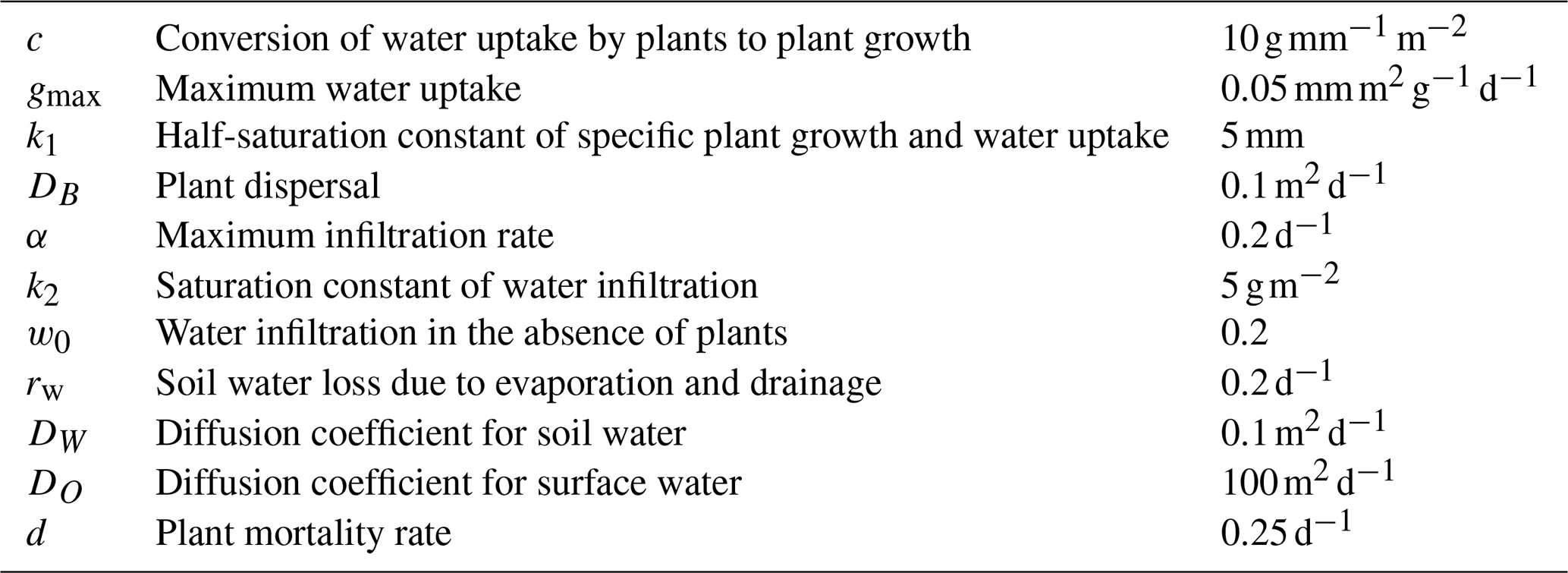
where Δ is the Laplacian operator and R is the rainfall [mm d⁻¹]. Rainfall is the external forcing of the system that we consider to be a spatially independent function. The first term in the biomass equation represents water uptake by the plant. The first term in the soil water equation is linked to the infiltration rate of water in the soil that is enhanced by the presence of biomass. The factors in front of the Laplacians (ΔB, ΔW, and ΔO) represent the diffusion constants of the different quantities. We consider a periodic domain of size l=100 m. The parameters are provided in Appendix A.

3 Effect of rainfall perturbation on vegetation dynamics: identifying critical timescales

We consider a spatially homogeneous perturbation applied to surface water, representing a decrease in rainfall across the entire domain. This type of perturbation is meaningful, as it mimics scenarios of prolonged droughts or gradual shifts in climate patterns. By applying different rates of change to a system that is initially in a high-rainfall state, we aim at identifying which critical factors influence the transient response of vegetation.

Previous research has highlighted the dependence of system solutions on the rate of environmental change, as common in open dynamical systems. In the context of vegetation patterns, different rates of rainfall decrease can lead to diverse outcomes, ranging from transitions to multi-pulse states to abrupt shifts to bare soil.

Starting from a high-rainfall situation ($R=\mathrm{1.4}\mathrm{mm}{\mathrm{d}}^{-\mathrm{1}}$), for which only the homogeneous vegetated state is stable, we decrease rainfall with different rates of change a [mm d⁻²]. Figure 1 shows the evolution of the spatial structure of the biomass (in green) as a function of rainfall, for different values of a. We find a transition from a homogeneous state to a heterogeneous distribution with two or three vegetation “pulses”, before it finally disappears. The sequence and timing of the transitions depend on a. For a rate of change of ${\mathrm{10}}^{-\mathrm{3}}\mathrm{mm}{\mathrm{d}}^{-\mathrm{2}}$, the system jumps directly from a homogeneous vegetated state to a bare-soil solution. The critical rate of change at which all vegetation is eradicated is ${\mathit{\tau }}_{R_{\text{tip}}}\sim \mathrm{1000}\mathrm{d}$.

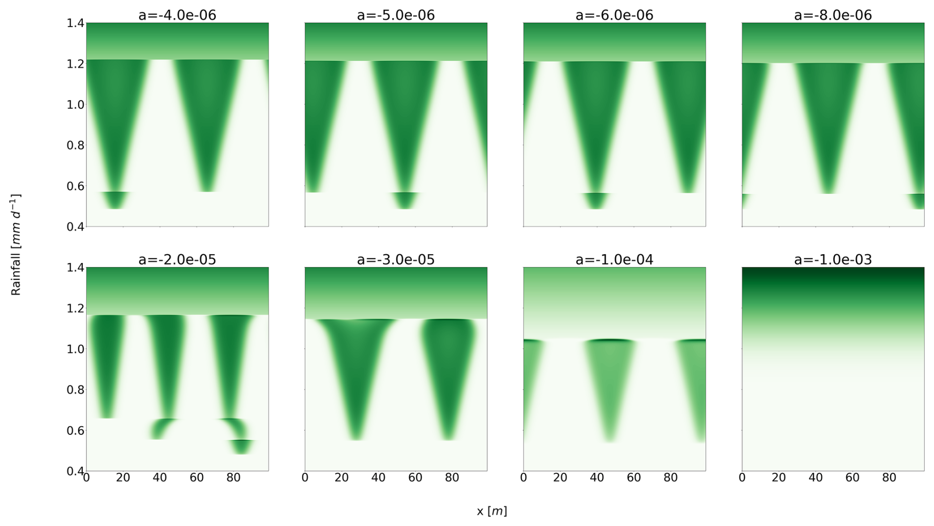
Figure 1 Sensitivity of the Rietkerk model to various rates of change in rainfall. Each panel represents a solution with a given rate of change a. The x axis is the spatial dimension, whereas the y axis is the rainfall. Every run has the same start and end point rainfall values, but they differ by the rate of change. Every simulation starts with a homogeneous vegetated state, which is the only stable equilibrium at this value of rainfall. For the last value of rainfall ($R=\mathrm{0.4}\mathrm{mm}{\mathrm{d}}^{-\mathrm{1}}$), the only stable equilibrium is the homogeneous bare-soil solution.

When reversing the rainfall gradient from low to high, the system follows a different transition path between low and high biomass. This hysteresis can be attributed to the range of precipitation where multiple stable equilibria exist in the Rietkerk model.

It is not surprising that the response depends on the rate of change. Ashwin et al. (2012) established general principles of so-called rate-induced tipping (R-tipping) in models based on ordinary differential equations, and rate-dependent responses were also described specifically in models of vegetation patterns (Siteur et al., 2014; Chen et al., 2015; Bastiaansen et al., 2020). However, the value of ${\mathit{\tau }}_{R_{\text{tip}}}$ is intriguing. Indeed, the timescale associated with the destruction of vegetation pulses is, through dimensional analysis, estimated to be ${\mathit{\tau }}_{\text{destruction}}=\frac{\mathit{\alpha }}{c{g}_{\text{max}}}{\left(\frac{R}{k_{\mathrm{2}}{g}_{\text{max}}}\right)}^{\mathrm{3}}\frac{\mathrm{1}}{d}=\mathrm{52}\mathrm{d}$.

This relationship is linked to the transfer of water to biomass, to vegetation mortality, and to rainfall. To test the dependence of the proposed scaling on rainfall, we conducted the following numerical experiments. Starting from a stable equilibrium consisting of two vegetation pulses at $R=\mathrm{1.2}\mathrm{mm}{\mathrm{d}}^{-\mathrm{1}}$, we abruptly reduced the rainfall to values of between 0.3 and 0.8 mm d⁻¹. This reduction leads to vegetation collapse, driving the system toward the bare-soil equilibrium. We then determined the destruction timescale by fitting an exponential function to the mean biomass evolution for different rainfall values. The resulting timescales are shown in Fig. 2b. Our results reveal a cubic relationship between the destruction timescale and rainfall, supporting the validity of our scaling.

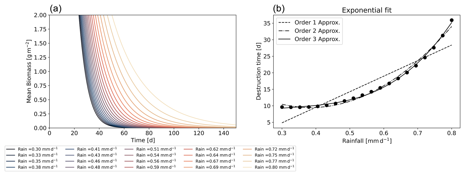
Figure 2 Panel (a) shows the mean biomass over time for rainfall values ranging from 0.3 to 0.8 mm d⁻¹. Panel (b) displays the destruction timescales obtained from an exponential fit as a function of rainfall, along with polynomial fits of the destruction timescale of orders 1, 2, and 3.

Having a ${\mathit{\tau }}_{R_{\text{tip}}}$ value that is about 30 times that of τ_destruction suggests that a slower process dominates the system's behaviour under changing environmental conditions. Bastiaansen et al. (2020) already identified another critical timescale within the Klausmeier model (Klausmeier, 1999). It is linked to the movement of pulses towards a stable, regular state. This concept is crucial for understanding vegetation dynamics in response to gradual environmental changes.

We now proceed to determine a similar timescale in the Rietkerk et al. (2002) model and will call it the rearrangement timescale, τ_rear. First, we perform a numerical experiment in which a pulse is removed for a given rainfall value, and the time taken for the system to stabilize is computed. Figure 3 shows the results for different rainfall values. We find that τ_rear∼1000 d. This rearrangement timescale is of the same order as ${\mathit{\tau }}_{R_{\text{tip}}}$, suggesting a fundamental connection between the two. This correspondence would also support that R-tipping is conditioned by the slowest timescale in the system. The rearrangement timescale effectively represents this slow process, dictating the system's overall response to changing conditions. Second, we attempt to link this rearrangement timescale to quantities in the system. Inspired by the scaling proposed in Bastiaansen and Doelman (2019), we assume that the movement of pulses is determined by diffusion coefficients. Specifically, we take the advantage of the fact that the ratio between the slow and the fast diffusion coefficients in the reaction–diffusion model drives the creation of the patterns (Murray, 2003; Meron, 2015). For the Rietkerk model, the fast component is the surface water (O), whereas the slow components are the biomass (B) and the soil water (W). Hence, we propose the following scaling for the rearrangement time ${\mathit{\tau }}_{\text{rear}}=\frac{\mathit{\alpha }}{c{g}_{\text{max}}}{\left(\frac{R}{k_{\mathrm{2}}{g}_{\text{max}}}\right)}^{\mathrm{3}}\frac{\mathrm{1}}{d}\sqrt{\frac{D_O}{D_B}}\sim \mathrm{1000}\mathrm{d}$. The key factor determining the rearrangement time appears to be the square root of the ratio between the diffusion coefficients of the fast and slow variables. To verify this, we perform a series of experiments in which the diffusion coefficient of the slow variables (biomass and soil water) varied by a factor f. To obtain a stabilization time for the different values of f, we run a series of numerical experiments similar to the one presented earlier. We start from a stable state for a given value of rainfall and f, and we then remove one pulse of vegetation. We compute this stabilization time for different values of rainfall and take the larger stabilization time because it is the one that is of interest regarding R-tipping. The results are presented in Fig. 4. The rearrangement timescale that is diagnosed numerically fits the theoretical curve proposed for τ_rear fairly well.

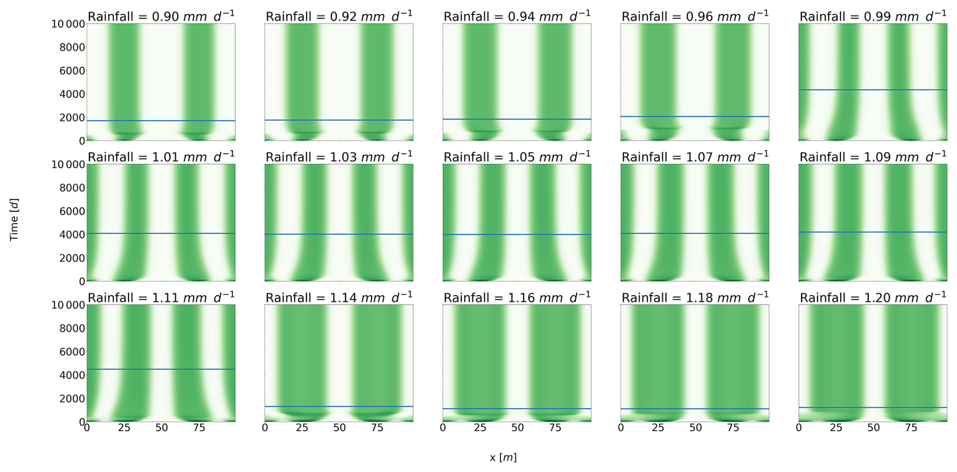
Figure 3 Rearrangement timescale with respect to rainfall. Each panel represents the solution of the following numerical experiments; we start at stable equilibrium with four pulses and then remove one pulse. For each experiment, we then identify the time until the system reaches a new equilibrium by moving around the pulses. This time is shown by the horizontal blue line in each panel.

This finding highlights the critical role of the rearrangement timescale in determining the system's response to environmental changes. Specifically, it emphasizes the need to account for this slower timescale when analysing vegetation dynamics. Understanding and quantifying this timescale provides valuable insights into the resilience and stability of vegetation systems under gradual environmental shifts.

4 Effect of spatially and temporally structured noise on vegetation pattern resilience

The kind of perturbation applied to the system is an important aspect of resilience diagnosis (Kéfi et al., 2019); specifically, the spatial scale of the perturbation must be considered. In the following section, we consider a dynamic perturbation consisting of a spatially distributed noise modelled mathematically as a Gaussian stochastic process with a mean $\mathbb{E}\left[\mathit{\xi }\right(t,x\left)\right]=\mathrm{0}$ and standard deviation σ=0.1. The temporal structure is that of an Ornstein–Uhlenbeck process. The correlation function is $\mathbb{E}\left[\mathit{\xi }\right(t,x\left)\mathit{\xi }\right(s,y\left)\right]={\mathrm{e}}^{-|t-s|/{\mathit{\lambda }}_t}{\mathrm{e}}^{-(x-y{)}^{\mathrm{2}}/{\mathit{\lambda }}_s^{\mathrm{2}}}$.

Stochastic perturbations are applied to the biomass (B) and surface water (W). Formally, the model takes the following form:

$$\begin{array}{ll}{\displaystyle \frac{\partial B}{\partial t}}& {\displaystyle }=c{g}_{\text{max}}{\displaystyle \frac{WB}{W+k_{\mathrm{1}}}}-dB+D_B\mathrm{\Delta }B+{\mathit{\xi }}_B(x,t),\\ {\displaystyle \frac{\partial W}{\partial t}}& {\displaystyle }=\mathit{\alpha }O{\displaystyle \frac{B+k_{\mathrm{2}}{w}_{\mathrm{0}}}{B+k_{\mathrm{2}}}}-g_{\text{max}}{\displaystyle \frac{WB}{W+k_{\mathrm{1}}}}-r_{\mathrm{w}}W+D_W\mathrm{\Delta }W,\\ \text{(2)}& {\displaystyle \frac{\partial O}{\partial t}}& {\displaystyle }=R-\mathit{\alpha }O{\displaystyle \frac{B+k_{\mathrm{2}}{w}_{\mathrm{0}}}{B+k_{\mathrm{2}}}}+D_O\mathrm{\Delta }O+{\mathit{\xi }}_O(x,t),\end{array}$$

where ξ_O(x,t) and ξ_B(x,t) are independent noise processes. For biomass, we consider an autocorrelation timescale of 1 d, and different autocorrelation length scales (λ_biomass,s) are tested. For surface water, the perturbation is homogeneous in space, and different autocorrelation timescales λ_rainfall,t are tested.

Figure 5 summarizes the stationary response of the model to λ_biomass,s and λ_rainfall,t, considering the mean biomass. Outputs reported on those tables are the average of 15 experiments. First, we consider the spatial structure of the noise, applied to the biomass. We focus on the horizontal lines of the tables, one by one, with the structure of the perturbation changing from highly heterogeneous to almost homogeneous as each line is browsed from the left to the right (increasing λ_biomass,s). We find that mean biomass tends to decrease as spatial autocorrelation increases, and this occurs regardless of the choice of time autocorrelation. This suggests that more homogeneous stochastic perturbations tend to destroy more biomass and send the system towards the bare-soil equilibrium. Thus, the resilience of the vegetation is reduced if the perturbation is spatially more homogeneous.

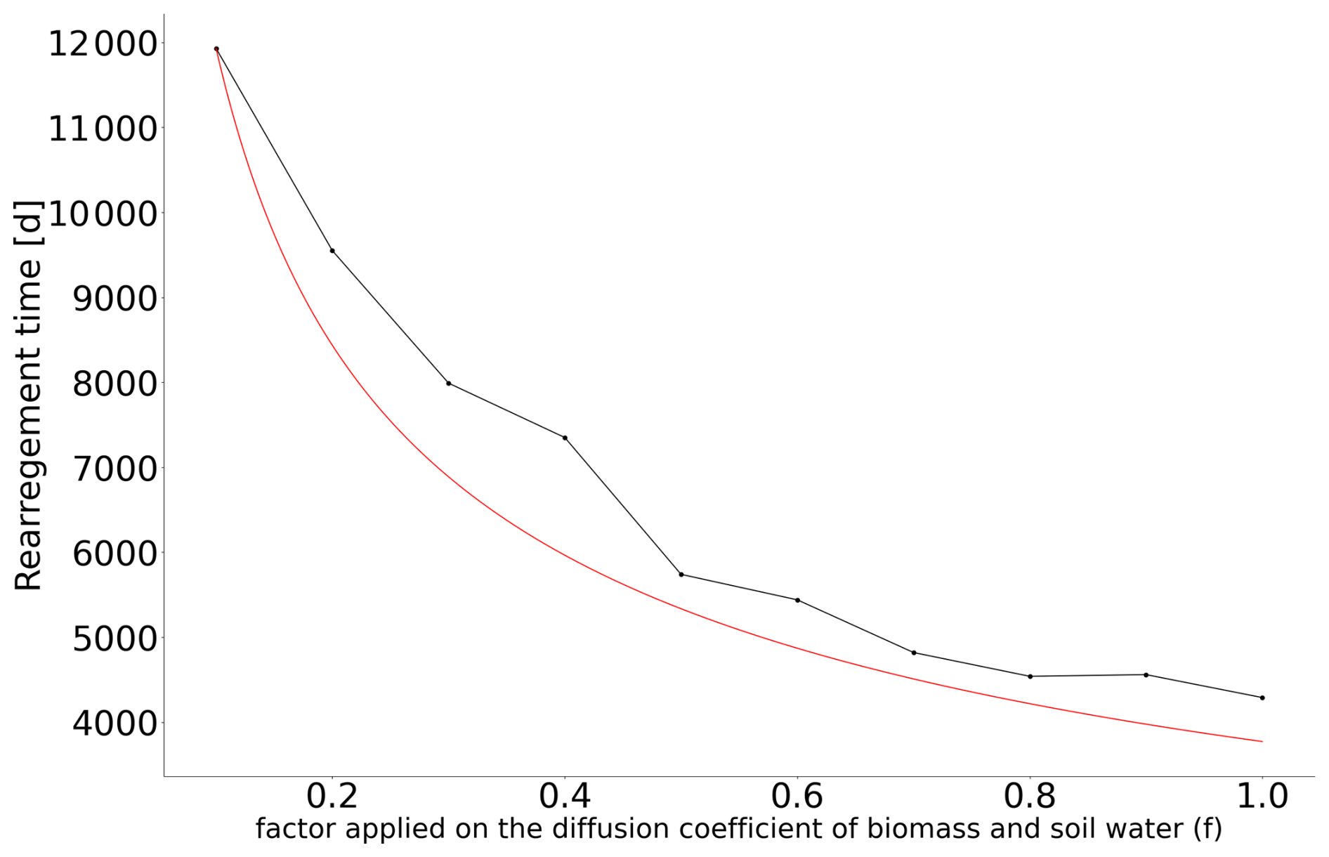
Figure 4 Link between the factor f applied on the diffusion coefficient of the slow components (biomass and soil water) and the rearrangement timescale. This timescale is estimated by finding a stable equilibrium for the new diffusion coefficients, removing one of the pulses, and then estimating the stabilization time. This procedure is applied for different values of rainfall, and we take the largest stabilization time into account. The results are shown using black dots, and the red line scales as $\frac{\mathrm{1}}{\sqrt{x}}$.

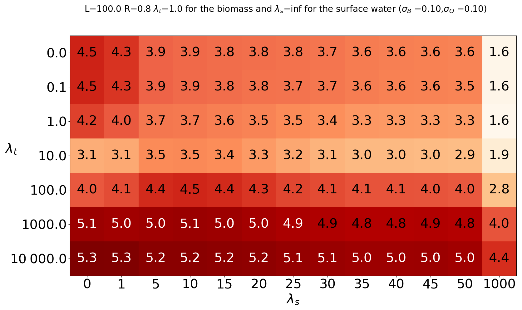
Figure 5 Summary table for the runs with stochastic forcing. For each cell, we ran the model 15 times with the same λ_t and λ_s. The table indicates the ensemble mean of the temporal mean of the spatial mean.

Second, we now focus on the time correlation of the stochastic perturbation of surface water. We find that both the spatial mean and the variance reach a minimum at λ_t=10 d. This timescale is the τ_destruction timescale previously identified in the scaling analysis. This suggests a form of resonance associated with τ_destruction preventing self-organization of vegetation. On the other hand, biomass reaches a maximum for a perturbation timescale of 1000 d, coinciding with the rearrangement timescale τ_rear that we also identified in the scaling analysis.

To visualize the behaviour for those different values of temporal autocorrelation, we show, in Fig. 6, realizations representative of the general behaviour, for four values of λ_t. We see that patterns tend to disappear for λ_t=10 d and reappear for λ_t=1000 d. The ability of the system to maintain (or not maintain) patterns, depending on the timescale of the perturbation, explains the variation in mean biomass observed in Fig. 4. We suggest that the slow stochastic perturbation is more effective at moving the system gently around the states associated with the highest biomass, without destroying patterns. The slow timescale (rearrangement timescale) is intrinsically linked to the spatial extent of the model. It would not exist in a zero-dimensional analysis. In this respect, we have already noted that non-linear, spatially extended systems tend to have multiple equilibria for a given input – here, a given rainfall. The multiplicity of equilibria, whether they are stable or not, increases the resilience of the system in the sense of Holling (1973). Metaphorically, such equilibria may be seen as tree branches in a forest to which an orangutan might cling to avoid falling. This phenomenon is clearly visible in Fig. 7, displaying the time evolution of the biomass with a fixed rainfall of 0.8 mm d⁻¹. In this configuration, we see that the system jumps from one configuration of pulses to another, passing from two to three pulses or vice versa. The transition, associated with the vanishing or the creation of a pulse, happens quickly, with a timescale of a few days. We again find the τ_destruction (fast) timescale identified earlier. Those configurations correspond to stable equilibria for the chosen rainfall as previously identified (Zelnik et al., 2013; Vanderveken et al., 2023). The two- and three-pulse configurations are not the only states being visited by the system. Occasionally, a configuration emerges consisting of a large pulse accompanied by a smaller one. The latter does not correspond to an equilibrium for a rainfall value of 0.8 mm d⁻¹, but it can be interpreted as the “ghost” of a mixed state identified in Vanderveken et al. (2023). Mixed states are always unstable and exhibit pulses with different heights. The mixed state that interests us here is the one with one big pulse and one small pulse. Its existence spans from 0.6 mm d⁻¹ to less than 0.8 mm d⁻¹. In the stochastic realization, the position of the second small pulse is not perfect because of noise. We clearly see that even if this mixed state with two pulses is not an equilibrium for this value of rainfall, it plays a role in the dynamics – hence the qualifier of ghost (Hastings et al., 2018; Morozov et al., 2020). Ghost attractors and unstable equilibria expand the resilience of the system because, in view of the orangutan in the forest, these configurations are new tree branches to cling to.

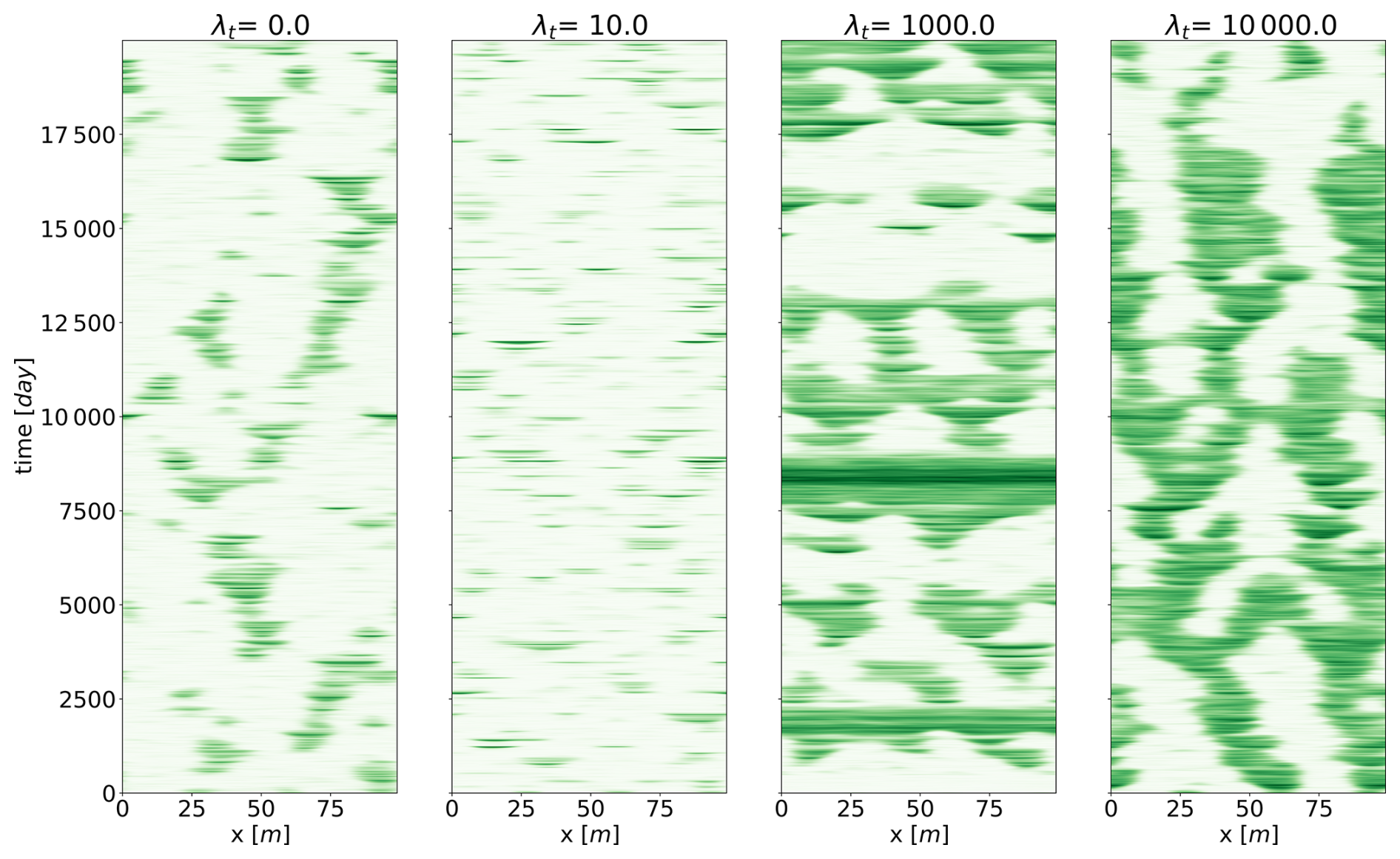
Figure 6 Four realizations of the stochastic Rietkerk model with λ_s=1 m. Biomass is the variable shown. Each panel presents a representative realization with different temporal autocorrelations (λ_t).

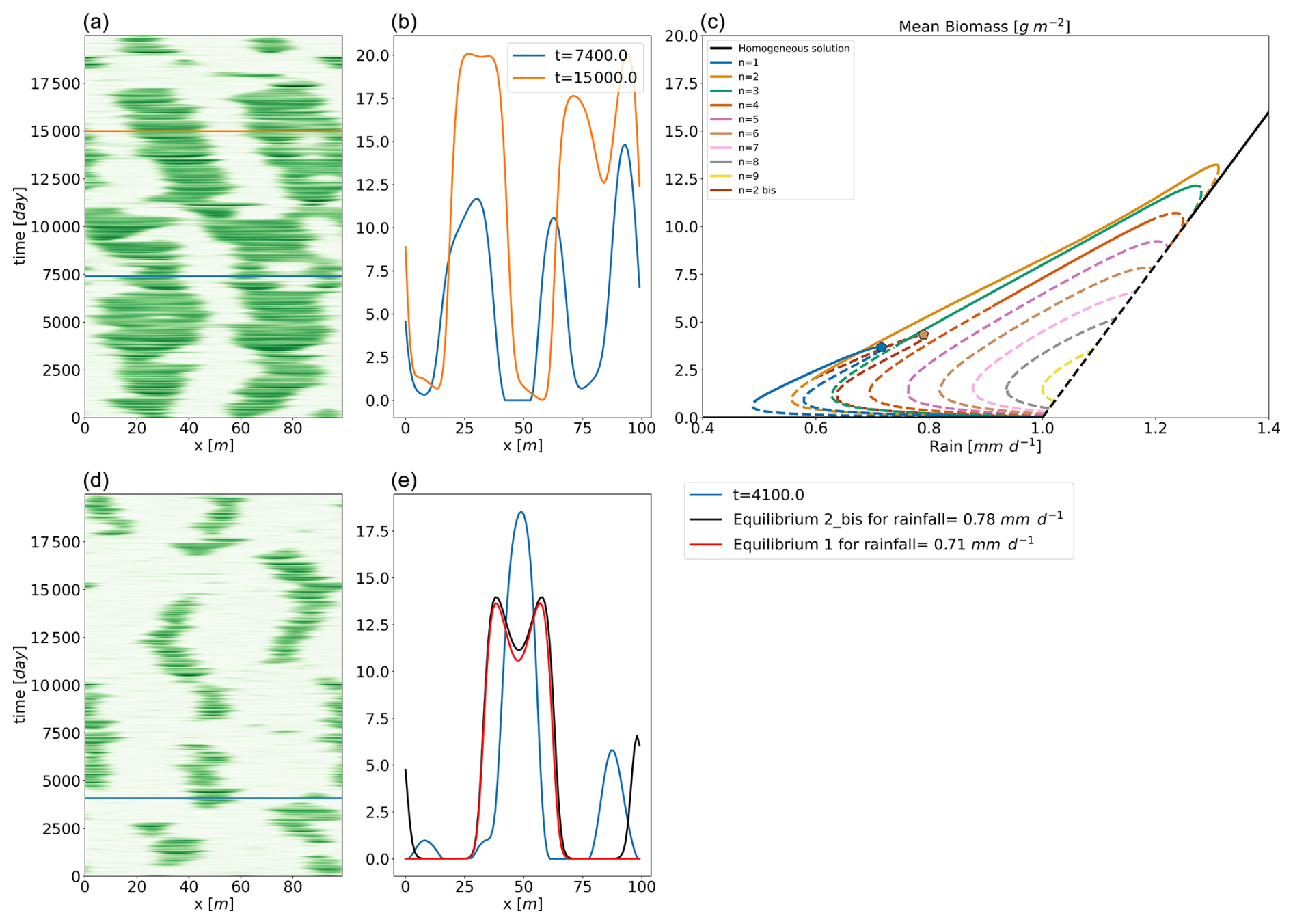
Figure 7 Two realizations of the stochastic Rietkerk model with different types of noise. In panel (a), the parameters are $R=\mathrm{0.8}\mathrm{mm}{\mathrm{d}}^{-\mathrm{1}}$, λ_t=1 d, and λ_s=10 m for the noise applied on the biomass, and λ_t=10 000 d and is spatially homogeneous for the noise applied on the surface water. In panel (d), the parameters are $R=\mathrm{0.8}\mathrm{mm}{\mathrm{d}}^{-\mathrm{1}}$, λ_t=1 d, and λ_s=15 m for the noise applied on the biomass, and λ_t=1 d and is spatially homogeneous for the noise applied on the surface water. The three horizontal lines mark the timing of the snapshots represented in panels (b) and (e) respectively. Panel (c) gives the bifurcation diagram, with two pentagons marking the position of two equilibria shown in panel (e).

In this study, we focused on the effect of spatial and temporal correlations on the system. To assess the impact of noise amplitude, we performed numerical experiments for low-noise-intensity (σ=0.09) and high-noise-intensity (σ=0.3 and σ=0.9) levels. We observed that the results are consistent for a low value of noise amplitude.

For σ=0.3, we observe pattern destruction at λ_t=1 d, followed by pattern reappearance at higher values of temporal autocorrelation. At σ=0.9, all patterns are destroyed, and the system stabilizes into a spatially homogeneous solution oscillating with rainfall.

Regarding mean biomass, we observed a consistent increase with increasing temporal autocorrelation for both σ=0.3 and σ=0.9. This behaviour can be understood by two complementary numerical experiments.

First, we applied noise exclusively to the surface water, using three values of σ=0.1, 0.3, and 0.9. For σ=0.1, biomass is eliminated at λ_t=10 d. For higher noise amplitudes, two phenomena emerge: (1) the range of temporal autocorrelation over which biomass is reduced shifts to lower values of λ_t; (2) the mean biomass increases significantly at higher λ_t. Together, these effects result in an increase in biomass with increasing temporal autocorrelation.

Second, we applied noise exclusively to the biomass components, using the same three values of σ and fixing temporal autocorrelation at λ_t=1 d. In this set-up, we observe that mean biomass increases with σ. This can be attributed to the nature of the Gaussian noise applied. Gaussian noise is symmetric, and as biomass is constrained to be non-negative, the system benefits more from the positive phases of the noise while being less affected by the negative phases. As the amplitude of the noise increases, this asymmetry leads to an overall increase in biomass.

The combined effects of noise applied to both surface water and biomass explain the observed increase in mean biomass for σ>0.1. However, the destruction and reappearance of patterns remain robust even at higher noise amplitudes (e.g. σ=0.3). At sufficiently high noise intensity (σ=0.9), a saturation effect occurs, and the system becomes entirely noise-driven, with patterns fully suppressed.

By demonstrating that resilience is bolstered by spatially heterogeneous noise and identifying critical timescales that influence biomass dynamics, we have provided valuable insights into the mechanisms underpinning ecological stability. Our findings emphasize the necessity of considering both stable and metastable states in resilience assessments, offering a more comprehensive understanding of ecosystem dynamics under varying perturbation regimes.

5 Conclusions

The present study explored the effects of a spatially homogeneous perturbation, specifically a decrease in rainfall, on vegetation dynamics in a model system. By varying the rate of change in rainfall, we observed significant differences in the system's response. At slower rates, the system transitions through multiple stable states, including two- and three-pulse solutions. However, a critical rate of change at ${\mathrm{10}}^{-\mathrm{3}}\mathrm{mm}{\mathrm{d}}^{-\mathrm{2}}$ results in a direct shift from a homogeneous vegetated state to bare soil. This critical rate of change aligns with a critical timescale ${\mathit{\tau }}_{R_{\text{tip}}}\sim \mathrm{1000}\mathrm{d}$, which is much longer than the pulse destruction timescale τ_destruction=52 d, highlighting the dominance of slower processes in the system's behaviour under environmental changes.

5.1 Rearrangement timescale and system resilience

We identified a critical rearrangement timescale τ_rear∼1000 d, which corresponds to the system's response time to structural changes, such as the removal of a vegetation pulse. This timescale is pivotal for understanding the resilience and stability of vegetation patterns. By linking τ_rear to the diffusion coefficients of the system's components, we derived a scaling law that accurately predicts the rearrangement time, emphasizing the importance of spatial interactions in determining system dynamics.

5.2 Impact of spatial and temporal noise

We further investigated the resilience of the system under spatial and temporal noise, modelled as Gaussian stochastic processes. The experiments demonstrated that the spatial autocorrelation of noise significantly impacts pattern formation. Higher spatial correlation leads to reduced spatial variance and biomass, suggesting that more homogeneous noise disrupts vegetation patterns. Temporal noise analysis revealed critical timescales – particularly around 10 and 1000 d – corresponding to the pulse and rearrangement timescales respectively. These findings underscore the intricate balance between spatial and temporal scales with respect to maintaining vegetation resilience.

5.3 Broader implications and multiple equilibria

Our analysis highlights the existence of multiple equilibria and the crucial role of slow timescales in spatially extended systems. The presence of ghost attractors and unstable equilibria broadens the system's resilience, offering additional configurations for the system to cling to, akin to tree branches in a forest. This multiplicity of stable and transient states enhances the system's capacity to adapt to gradual environmental changes, aligning with the concept of resilience as defined by Holling (1973).

In summary, this study contributes to clarifying the complex interplay between rainfall perturbations, spatial and temporal noise, and vegetation dynamics. By identifying critical timescales and exploring the system's response to various perturbations, we provide valuable insights into the resilience and stability of vegetation systems. These findings contribute to a deeper understanding of ecological dynamics and the factors influencing the persistence of vegetation patterns under changing environmental conditions.

Appendix A: Model parameters

The parameters are as in Rietkerk et al. (2002); see Table A1.

Table A1 Parameters for the Rietkerk model.

Appendix B: Structured noise

The noise used in this paper is correlated in both time and space. We prescribe its standard deviation (σ), length of spatial autocorrelation (λ_s), and time correlation (λ_t) with a period of L. To produce this noise, first, we compute the square root of the following covariance matrix, where N=100 is the number of spatial points:

$${\displaystyle }{\mathbf{A}}_{i,j}=max\left({\mathrm{e}}^{\frac{-(x_i-x_j{)}^{\mathrm{2}}}{{\mathit{\lambda }}_s^{\mathrm{2}}}},{\mathrm{e}}^{\frac{-(L-|x_i-x_j|{)}^{\mathrm{2}}}{{\mathit{\lambda }}_s^{\mathrm{2}}}}\right).$$

Then, we use an AR1 process (auto regressive process of order 1) in time to create the time dependence of the noise:

$${\displaystyle }{x}_{i,j}=x_{i,j}+\left(-c*x_{i,j}\mathrm{d}t+\sqrt{\mathrm{d}t}{\mathit{\sigma }}_e\sum _{k=\mathrm{1}}^n{\mathbf{A}}_{j,k}{\mathit{ϵ}}_k\right),$$

where $c=\mathrm{1}/{\mathit{\lambda }}_t$, dt is the time step, ${\mathit{\sigma }}_e=\mathit{\sigma }\sqrt{\mathrm{2}c}$, and ϵ_k is a Gaussian random variable of 0 mean and variance 1.

The resulting noise is exemplified in Fig. B1, and the temporal and spatial structure are shown in Fig. B2.

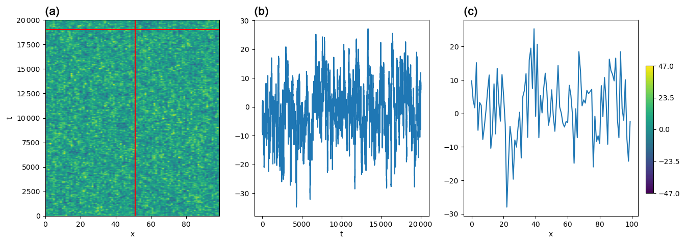
Figure B1 One realization of the structured noise with σ=10, λ_t=100, and λ_s=1. Panel (a) shows the full noise. The vertical red line and the horizontal red line mark the position of the snapshots; those snapshots are represented in panel (b) for the vertical snapshot and in panel (c) for the horizontal snapshot.

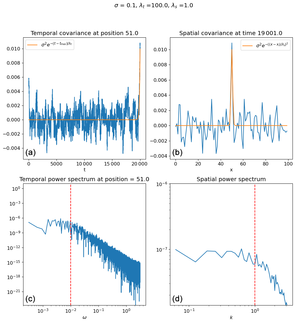
Figure B2 Mean over 50 realizations of the structured noise with σ=10, λ_t=100, and λ_s=1. In panel (a), the blue line is the mean over all the realizations with temporal autocorrelation at t=20 000, and the orange line is the theoretical expectation. In panel (b), the blue line is the mean over all the realizations of the spatial autocorrelation at x=50, and the orange line is the theoretical expectation. In panel (c), the blue line is the mean temporal power spectrum, and the vertical dashed red line is at $\mathrm{1}/{\mathit{\lambda }}_t$. In panel (d), the blue line is the mean spatial power spectrum, and the vertical dashed red line is at $\mathrm{1}/{\mathit{\lambda }}_s$.