the Creative Commons Attribution 4.0 License.
the Creative Commons Attribution 4.0 License.
 | 13 Feb 2024
A two-fold deep-learning strategy to correct and downscale winds over mountains
Louis Le Toumelin
Isabelle Gouttevin
Clovis Galiez
Nora Helbig
Assessing wind fields at a local scale in mountainous terrain has long been a scientific challenge, partly because of the complex interaction between large-scale flows and local topography. Traditionally, the operational applications that require high-resolution wind forcings rely on downscaled outputs of numerical weather prediction systems. Downscaling models either proceed from a function that links large-scale wind fields to local observations (hence including a corrective step) or use operations that account for local-scale processes, through statistics or dynamical simulations and without prior knowledge of large-scale modeling errors. This work presents a strategy to first correct and then downscale the wind fields of the numerical weather prediction model AROME (Application of Research to Operations at Mesoscale) operating at 1300 m grid spacing by using a modular architecture composed of two artificial neural networks and the DEVINE downscaling model. We show that our method is able to first correct the wind direction and speed from the large-scale model (1300 m) and then accurately downscale it to a local scale (30 m) by using the DEVINE downscaling model. The innovative aspect of our method lies in its optimization scheme that accounts for the downscaling step in the computations of the corrections of the coarse-scale wind fields. This modular architecture yields competitive results without suppressing the versatility of the DEVINE downscaling model, which remains unbounded to any wind observations.
- Article
(7641 KB) - Full-text XML
-
Supplement
(570 KB) - BibTeX
- EndNote


Understanding the declination of synoptic winds at a local scale in complex terrain is crucial for a wide range of applications, including assessing the dispersion of pollutants, predicting wildfire spread, and evaluating wind energy potential (Giovannini et al., 2020; Wagenbrenner et al., 2016; Dujardin and Lehning, 2022). Local winds also have a significant impact on the evolution of the snowpack. The high variability of wind fields in complex terrain generates local gradients in the surface energy balance, which in turn influences the interaction between the snowpack and the atmosphere. These interactions can lead to significant spatial variability in the seasonal snowpack at the slope scale (Mott et al., 2018). In addition, wind can cause snow redistribution in snow-covered areas through erosion and deposition processes, which is a major concern for avalanche hazard prediction (Lehning and Fierz, 2008).
Wind field variability at a local scale in mountains is largely driven by two factors: terrain forced flow, which refers to the direct impact of topography on large-scale winds, and thermally driven flows, which result from local temperature gradients caused by terrain inhomogeneity and variable shading (Whiteman, 2000). Terrain forced flow and thermal winds interact with each other, causing local variations in both speed and direction, making it challenging to understand and model mountain winds.
Many applications rely on the ability of numerical weather prediction (NWP) systems to model synoptic-scale wind fields above mountains (Quéno et al., 2016; Vionnet et al., 2016). NWP models are generally characterized by their horizontal grid spacing on the order of 1 km or several kilometers. Despite constant increases in horizontal resolution in recent years, a large number of use cases still require downscaling techniques to reach their resolution of interest (Vionnet et al., 2021; Marsh et al., 2020).
Several methods have emerged to adapt the wind fields provided by NWP systems (in this work referred to as “large scale”) to a local scale. Statistical downscaling is a family of methods that adapt large-scale information, such as NWP outputs, to local-scale specificities using statistical operations. Another approach, dynamical downscaling, relies on models to directly simulate atmospheric and surface processes at a higher resolution. A large variety of statistical downscaling methods can be found in the literature: e.g., Dupuy et al. (2021) and Goutham et al. (2021) develop statistical downscaling methods specifically tailored to operate at specific individual locations (their calibration sites). In a different way, Zamo et al. (2016) and Höhlein et al. (2020) adapt large-scale NWP wind fields to specific target grids at a higher resolution. By contrast, more general methods such as in Winstral et al. (2017) can theoretically be applied to any area with the inclusion of appropriate terrain descriptors as inputs. These methods not only increase the resolution of the simulated variables, but they also include corrective terms that can compensate for systematic errors in NWP modeling: this is a direct consequence of the use of an optimization or training step that links modeled data to wind observations. Such methods can also be referred to as model output statistics (MOS) or bias-correction methods and frequently present favorable statistics when evaluated using observed wind data. Since statistical relationships are derived by linking outputs from a specific NWP system to observed values, two challenges emerge. First, their use is restricted to a unique NWP system or NWP system version. Second, the model capability to extrapolate wind values to areas where no calibration has been performed can be challenging and must be rigorously assessed.
Conversely, other downscaling methods restrict their use to the modeling or parameterization of local-scale processes only, without any optimization based on observations. These methods may improve evaluation metrics through the added value of the representation of missing processes; however, they do not compensate for systematic errors in large-scale modeling and hardly compete in terms of evaluation metrics with methods including a corrective step. However, their use is not restricted to any specific NWP or to any specific geographic area. A large array of the aforementioned models can be found in the literature, ranging from simple statistical relationships (Liston and Elder, 2006; Helbig et al., 2017) to dynamical downscaling methods including atmospheric models of various complexities (Wagenbrenner et al., 2016; Raderschall et al., 2008; Vionnet et al., 2017). DEVINE (Le Toumelin et al., 2023) is a brand-new example of statistical downscaling models that represent wind fields at a local scale without incorporating any fit to observed data. Indeed, DEVINE simulates the adaptation of large-scale wind fields to high-resolution terrain (30 m) by using a fully convolutional neural network. More specifically, this model was trained to replicate the behavior of the atmospheric model ARPS (Advanced Regional Prediction System) over complex Gaussian topographies (Helbig et al., 2017).
Consequently, systematic errors originating from the NWP large-scale inputs can eventually be transferred and amplified through DEVINE. These errors can have a variety of origins, like missing or imperfect parameterizations, overly coarse model topography, and errors due to the assimilation procedure. Furthermore, the use of a downscaling model also makes it difficult to determine the origin of the modeling errors: whether the downscaling model accurately or inaccurately simulates local-scale processes or whether error compensations between the large-scale forcing and the downscaling model scramble the evaluation. However, even though error attribution is complex, identifying typical weather and topographic situations where inputs or downscaled data are incorrect is more accessible, notably thanks to deep learning.
As an illustration, Le Toumelin et al. (2023) observed that AROME (Application of Research to Operations at Mesoscale, an operational numerical weather prediction system used by Météo-France) wind fields are frequently underestimated in elevated and exposed areas. After using DEVINE, they noted smaller errors: thanks to the ability of the downscaling model to simulate terrain forced flow at a local scale and notably strong wind accelerations over summits and crests, the initial NWP underestimation is reduced. Since some wind speed underestimation remains, it is not clear whether the downscaling model does not accelerate the input wind sufficiently or whether the initial NWP wind speeds are too low. Whatever their origin, deep-learning techniques together with in situ measurements and ancillary atmospheric and topographic data may enable an a posteriori compensation of such systematic biases.
In this context, we design and present a strategy, based on deep learning, that corrects NWP input wind fields upstream of the DEVINE downscaling method. Indeed, the correction is made before the downscaling step, but the effect of downscaling is accounted for in the optimization of the neural networks' parameters that are responsible for the correction. In turn, most errors affecting the coarse-scale wind fields are corrected without affecting the spatial extrapolation capabilities of the downscaling model and diminishing the associated performances. By scrutinizing a set of variables including many variables that can influence air motion (e.g., temperature, humidity, boundary layer height) and advanced topographic metrics, the artificial neural networks developed for this correction optimize NWP wind speed and direction before calling the downscaling model. With this modular architecture, we provide an end-to-end chain including downscaling and model output statistics, which permits us to boost the evaluation performances of the DEVINE downscaling model.
In this study, we used forecasts from the AROME NWP system as inputs to our new downscaling strategy. We rely on forecasts from AROME for both large-scale wind fields and other atmospheric variables used in the corrective step. Our models also make use of high-resolution topographical information (30 m). Quality-controlled wind observations acquired over a large network of automatic weather stations (AWSs) are used for model training (training set) and evaluation (test set). We finally compared the performance of our models to the operational analysis of the AROME system.
2.1 AROME
The AROME NWP system embeds a limited-area model, notably run by Météo-France for short-term weather forecasting operations. It simulates the state of the atmosphere and the surface over a European domain including the French Alps, the Pyrenees and Corsica. The model solves the non-hydrostatic fully compressible Euler equations by using a semi-Lagrangian and semi-implicit numerical solver and by including a spectral representation of several prognostic variables (Seity et al., 2011; Bénard et al., 2010). The physics is inherited from the Meso-NH model (Lafore et al., 1998; Lac et al., 2018) and the dynamical core from ALADIN-NH (Bubnová et al., 1995). The model is driven at its borders by the Action de Recherche Petite Echelle Grande Echelle (ARPEGE) model. It simulates energy and mass exchanges between the atmosphere and the surface thanks to the SURFEX platform (Masson et al., 2013). Notably, AROME uses the SURFEX/ISBA model over land (Noilhan and Mahfouf, 1996; Masson et al., 2013) and the simplified snowpack scheme from Douville et al. (1995) over snow-covered areas. Since 2018, AROME has operated with a 1.3 km horizontal grid spacing over France, which is of great interest for applications that require high-resolution information about the state of the boundary layer such as weather forecasting over complex terrain (Quéno et al., 2016; Vionnet et al., 2016). The AROME system also includes a 3DVar assimilation scheme, which takes into account radial winds observed by radars in addition to the assimilation of 10 m wind speeds. We note that wind observations in complex terrain are frequently neglected for assimilation due to their lack of spatial representativity (Gouttevin et al., 2023). Eventually, their distance to the AROME initial guess can also lead to their exclusion of the assimilation cycle.
AROME analyses are produced every UTC hour, whereas the model is also run in forecast mode every 3 h. For this study, we built two different products from the aforementioned cycles. Firstly, we built a continuous time series by extracting +6 to +29 h AROME forecast lead times initialized with the analysis of 00:00 UTC, as in Quéno et al. (2016), Vionnet et al. (2016), and Le Toumelin et al. (2023). This was done as a way to obtain continuous time series typically used to force snow and surface models as in Quéno et al. (2016), Vionnet et al. (2016), and Gouttevin et al. (2023). In this way, we were able to construct a continuous time series of 11 variables from AROME forecasts between 1 September 2017 and 1 October 2020 at an hourly time step (AROMEforecast). The variables are detailed in Table 1, and their respective use is described in Sect. 3.3. For the same period, we extracted the same variables from the analysis cycles (AROMEanalysis), also at an hourly time step. Finally, we obtain two datasets from AROME: AROMEforecast is representative of forecasted atmospheric and surface conditions and AROMEanalysis is representative of an a posteriori product, giving the most plausible state of the atmosphere at the considered date. In the following study, AROMEforecast is used as inputs of the postprocessing and downscaling schemes, as it would be within an operational high-resolution forecast system, whereas AROMEanalysis serves as a reference “best” product to compare with.
Glorot and Bengio (2010)Kingma and Ba (2015)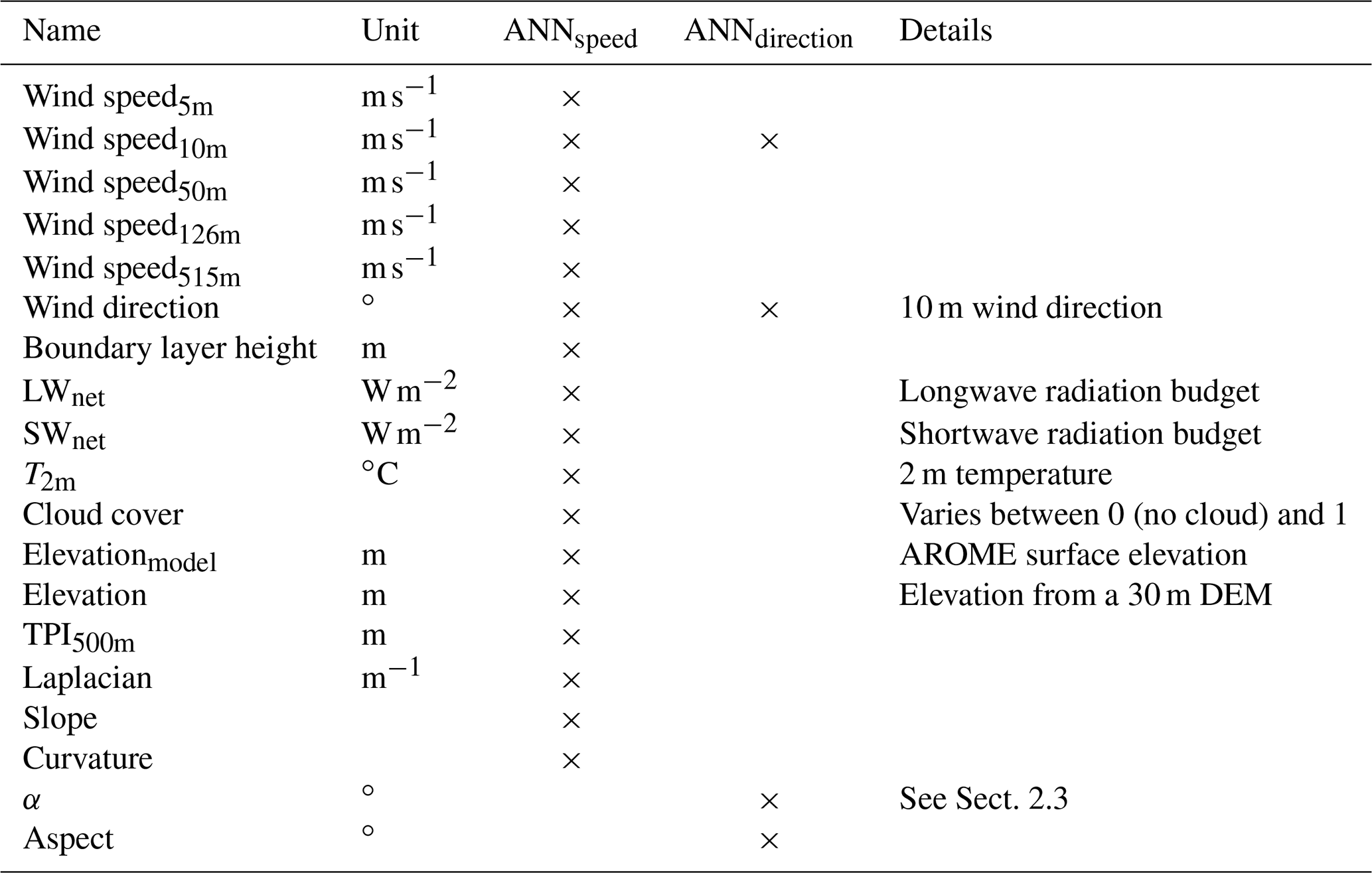
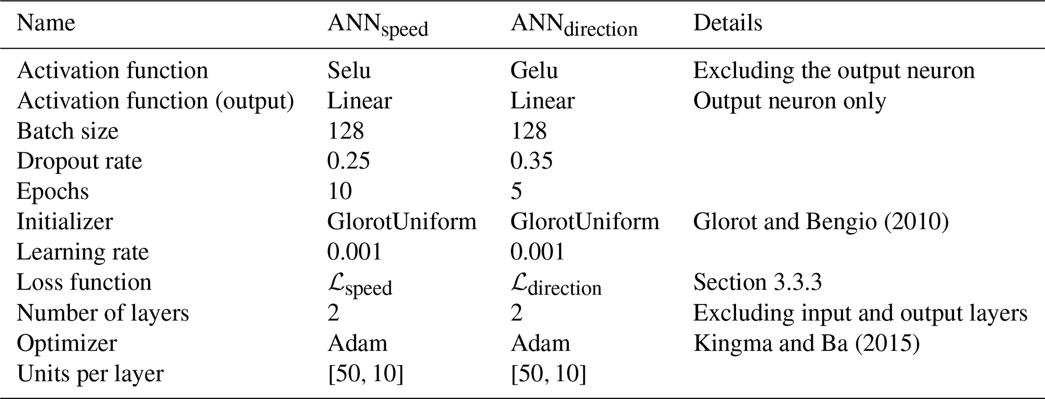
Table 2Architecture, hyperparameters and loss functions used in Neural Network and Neural Network+DEVINE.
2.2 Observations
We gathered hourly wind field observations from AWSs originating from different observation networks in Switzerland and France in order to train and evaluate our models (Fig. 1). In detail, we used a total of 273 observation stations. Of them, 214 are located in Switzerland and correspond to data provided by MeteoSwiss, the Swiss Federal Office of Meteorology and Climatology. Then, 59 stations are located in France, of which 54 are from Météo-France observational networks and 5 are from the GLACIOCLIM network (“Les GLACIers un observatoire du CLIMat” – “Glacier: an observatory of the climate”). We note the use of three AWSs from the Col du Lac Blanc instrumental site, a high-altitude observatory specifically dedicated to the study of mountain meteorology and drifting snow (Vionnet et al., 2017; Guyomarc'h et al., 2019). The observational sites are located in various types of environments, all representative of alpine terrain. This includes snow-covered areas, slopes, exposed terrain as well as lower-elevation valleys and some stations localized around urbanized terrain.
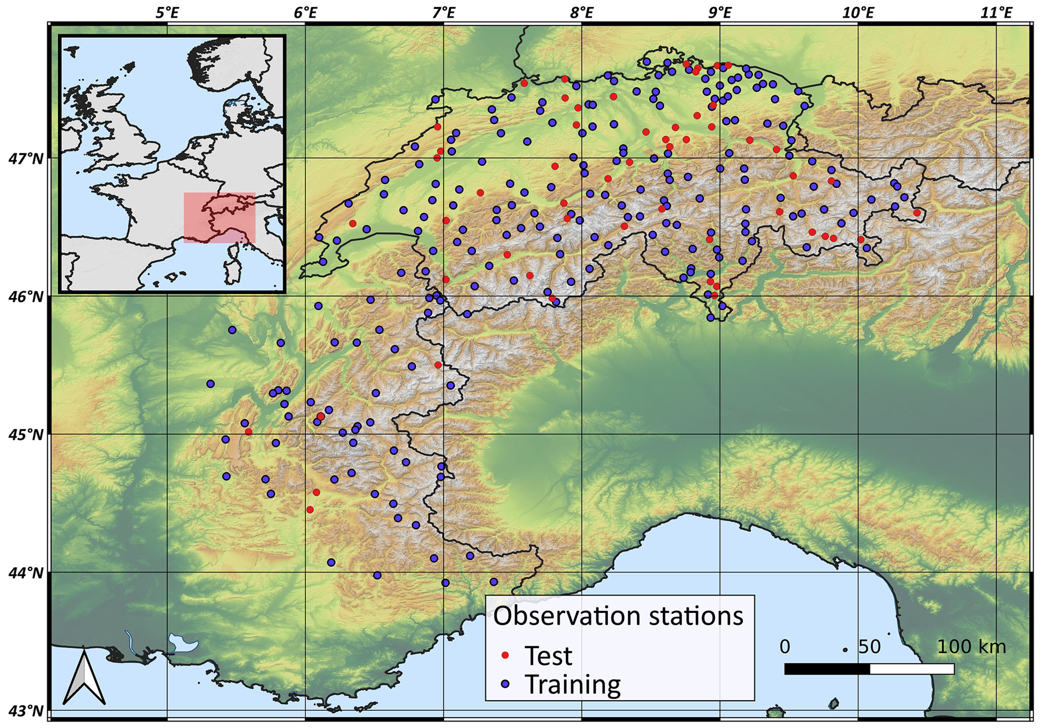
Figure 1In situ observation stations used to train the model (218 blue dots) and evaluate the model (55 red dots). All the stations are located in Switzerland and France. Train–test partitioning was performed using a stratified sampling method described in Sect. 3.4. Note that an additional dataset (not shown) comprising observations collected in Corsica and in the French Pyrenees has been used in Sect. 4.5 in order to evaluate the applicability of our model to other mountain ranges.
Since most of the wind observations used in this study were obtained in complex terrain and frequently under challenging meteorological conditions, we applied a quality-check procedure to our observational dataset, inspired by Lucio-Eceiza et al. (2018a, b). As extensively detailed in Le Toumelin et al. (2023), this procedure first asserts a correct data compilation and storage including chronological sorting, a search for eventual repeated dates, and the distinction between true north (360∘) and an undefined direction when wind speed is null (0∘). Moreover, it ensures the validity of observed speeds and directions by removing unrealistic observations (e.g., speeds >100 m s−1 or negative directions). The quality check also includes the use of log profiles to unify the observational height of wind fields (here set to 10 m) for measuring devices located below 10 m above the surface. This procedure uses snow height information when available to adjust wind profile correction. Moreover, some additional tests are designed to detect suspicious speeds or direction sequences. As an example, icing of wind sensors is a typical case of sensor dysfunction in complex terrain and is reflected by the acquisition of null or constant speeds and directions for several consecutive hours. The quality-check procedure also takes into account other typical suspicious sequences of data such as extremely high-speed variations (extreme spikes or lows in time series) and constant sequences of positive speeds for consecutive hours or days. Finally, longer-term rolling means are scrutinized to detect the suspicious rise or decline of observed mean speeds which can shed light on the occurrence of systematic errors of a diverse nature (e.g., mast tilting, new vegetation, or urbanization in the vicinity of the sensor).
2.3 Terrain parameters
Since the local topography has a large impact on wind fields, several topographic parameters are used as input variables for the corrective strategy so as to capture the dominant local features of the topography. Among the selected parameters, the TPI500m (Weiss, 2001) consists of computing the difference between a digital elevation model (DEM) pixel elevation and the mean elevation of neighboring pixels within a fixed radius (here taken at 500 m). Consequently, TPI500m gives an integrated vision of the relative elevation of the considered pixel: positive TPI500m indicates that the pixel of interest is higher than the neighboring pixels, and negative TPI500m indicates the opposite. The curvature, computed following Liston and Elder (2006), quantifies how much a terrain differs from a plane. The Laplacian, computed as in Le Toumelin et al. (2023), also gives an estimation of the local elevation variation and enables us to detect small-scale peaks or bowls within topographic maps. The slope, obtained as the root mean squared slope using first-order finite differences as in Helbig et al. (2017), quantifies the local slope of the topography. The aspect indicates the orientation of a pixel relative to the northerly direction. Finally, the parameter α, adapted from Dujardin and Lehning (2022), is computed following Eq. (1).
α is a proxy firstly indicating how wind direction should be modified in order to align perpendicularly to the aspect. Furthermore, α also increases with the slope, so that it is higher over steep slopes than over flat terrain. Similarly to the wind direction, α is expressed in degrees. Since α and aspect are computed using values from direct neighboring pixels, they tend to be sensitive to small-scale variations in topographic features. To reduce this variability, we averaged all aspects and α values using a 3×3 moving window, i.e., averaging all α values given the eight α values from the neighboring DEM pixels (30 m spaced). In this study, the DEM used was obtained after merging the RGE Alti DEM resampled to 30 m (IGN, 2013) inside of France's borders and the GLO-30 DEM in Switzerland (Fahrland et al., 2020).
3.1 Artificial neural network
Artificial neural networks (ANNs) are a specific type of machine-learning model. They are composed of interconnected units called neurons, which hold floating-point values, all organized into different layers. In a layer, neurons transmit the information received from the previous layer's neurons to the next layer's neurons. Communication consists first of an affine modification of each neuron value using weights (slope parameters) and biases (intercepts). Then, all neuron-modified values are summed and pass through a nonlinear activation function which produces the next layer's neuron input values. Finally, the first layer holds the raw inputs, while the last layer holds the predicted values. All weights and biases are typically initialized using random values and are then modified using optimization algorithms based on gradient descent methods. Such methods are based on the computation of the gradient of a loss function between the neural network output and the expected output with respect to the network weights and biases. Weights and biases are then optimized in the opposite direction of the gradient in order to minimize the loss. By replicating this strategy a large number of times over a large number of samples, artificial neural networks can learn complex patterns that link the training inputs to the training target outputs. Finally, we note the existence of different hyperparameters, which consist of parameters that are not weights and biases (e.g., the number of neurons and the number of layers). These parameters are not learned during the training process but are rather fixed independently.
3.2 DEVINE
DEVINE is a downscaling model based on a U-Net convolutional neural network (Ronneberger et al., 2015) designed to adapt wind fields to high-resolution topography (30 m) in complex terrain (Le Toumelin et al., 2023). This model takes as inputs high-resolution topography (30 m) and large-scale wind fields above the topography and provides three-dimensional wind fields with a 30 m grid spacing as output. DEVINE uses convolutions to detect advanced spatial features on topographic maps and to assemble them into more complex patterns within a latent space. This latent representation is then used to reconstruct high-resolution wind fields using spatial interpolation and convolutions to finally obtain wind simulations at the same resolution as the input topography. The model was trained using 7279 ARPS simulations performed by Helbig et al. (2017). These simulations were run over a large range of synthetic Gaussian topographies of diverse complexity using similar constant initial atmospheric conditions across all the simulations. The trained model showed good behavior at reproducing an ARPS simulation on an evaluation dataset. As a case study, Le Toumelin et al. (2023) applied DEVINE to downscale AROME-forecasted wind fields in the French Alps and used observations from 61 in situ stations for model evaluation. Qualitatively, the model simulates coherent spatial structures and notably simulates several characteristics of terrain forced flows. Notably, the model is able to detect ridges and summits and to simulate acceleration as observed within ARPS simulations that served as targets. Similarly, DEVINE shows good behavior in detecting windward and leeward areas and is able to modify speed accordingly. Some directional shifts were observed around topographic barriers (channeling) but remain modest. Some other features of mountain winds occurring at the slope scale such as recirculation areas or upslope and downslope thermal flows are not accounted for. Quantitatively, in addition to its spatial extrapolation abilities, DEVINE improves AROME evaluation metrics, notably at the most elevated and exposed stations. A significant improvement in modeling the highest wind speeds has also been observed, which is of great interest for applications requiring good precision above a certain speed threshold such as drifting-snow modeling.
3.3 Neural Network+DEVINE
3.3.1 Architecture
The model presented in this study corresponds to an extension of the DEVINE model. It consists of the addition of two ANNs that process large-scale NWP data and local-scale topographic data prior to the use of the DEVINE downscaling model. More precisely, a first neural network is designed to compute an additive correction for the NWP wind direction (ANNdirection) aiming at compensating for large-scale modeling errors, and a second network performs similar corrections for the NWP wind speed (ANNspeed). The modified large-scale wind speed and direction are then used to feed the DEVINE downscaling model, which also uses a high-resolution topographic map (30 m) of the area considered. In detail, ANNdirection uses 4 input variables (2 topographic parameters and 2 variables from the NWP system), and ANNspeed uses 17 variables (5 topographic variables and 12 NWP variables), all listed in Table 1. The outputs of the overall model (referred to as Neural Network+DEVINE) are the same as DEVINE outputs, i.e., high-resolution maps of the three components of the wind vector.
As ANNdirection and ANNspeed need to output wind speed and direction, they need to take into account the typical range of wind speed (positive values, generally below 100 m s−1) and direction values (0 to 360∘). To facilitate such a task, we used skip connections: considering ANNdirection (ANNspeed), the initial NWP direction (speed) is added to the value of the ANN's output neuron so that the network concentrates on the computation of a directional difference (speed difference) instead of computing the direction (speed) directly. Furthermore, care has to be taken with activation functions used before the skip connection: the direction difference (or speed difference) should not be constrained to positive or negative values only (as in relu functions for instance) since modifications can be either positive or negative depending on weather and topographic situations. Hence, we selected a linear activation function for the last layer of both input networks before calling the skip connection layer. Furthermore, after adding modifications suggested by the network to the initial wind direction (speed), i.e., after the skip connection layer, we had to ensure that no negative values were produced. For that, we used a relu activation function that caps negative values to zero. Hyperparameters and architecture details are summarized in Table 2. Diverse architectures and hyperparameters were tested in order to converge to the final model. We checked that our model does not overfit the test set by computing metrics using a three-fold cross-validation strategy presented in Table S1 in the Supplement.
3.3.2 Training
In order to adapt the weights and biases of the ANNs, we adopted a sequential approach. First, we optimized ANNdirection for wind direction, and then we optimized ANNspeed for wind speed. This order is motivated by the fact that an erroneous direction can translate into erroneous high-resolution wind speeds with DEVINE as a result of wrong topography adjustments, whereas the opposite will have less impact. We selected 218 training observation stations in the French Alps measuring wind speed and direction. Additionally, we used data from the nearest grid cell of AROME at each of these stations to take into account large-scale atmospheric conditions and extracted topographic maps around these observation stations to take into account topography. It is important to note that, in the end, our model outputs wind field maps, whereas observation stations provide information for isolated points in space. In order to optimize the neural networks, we selected a single wind value at the center of each simulated map that is compared to the corresponding target from the observation station. This step required us to accurately match the position of the center of the simulated map with the observation station: this was possible by providing input topographies to our model that were already centered on the location of the observation sites. The optimization process involved back-propagating the gradient of a loss function, which was computed using the wind direction or speed value simulated by DEVINE and the targets. The loss functions used in this study are described in Sect. 3.3.3 and correspond to a cosine distance for optimizations of the direction and a modified mean squared error for optimization of wind speed. During the optimization of ANNdirection, both DEVINE and ANNspeed weights and biases are kept frozen. Similarly, DEVINE and ANNdirection weights and biases are not updated during ANNspeed optimization. We note that DEVINE parameters were directly taken from the original model (Le Toumelin et al., 2023) and have not been modified in this study. This choice was made because our goal was to develop an optimization system to be used with DEVINE rather than fitting DEVINE to AROME wind fields. Modifying DEVINE weights would lead to the creation of a new and less versatile downscaling model (see Sect. 5) that assumes a specific type of input data (here AROME data), with potential limitations in its scope of applicability. Once trained, Neural Network+DEVINE can model wind fields at high resolution, even over areas not included in the training process. Additionally, intermediate values (i.e., ANN outputs, referred to as Neural Network) are saved for model interpretability purposes (red dots in Fig. 2).
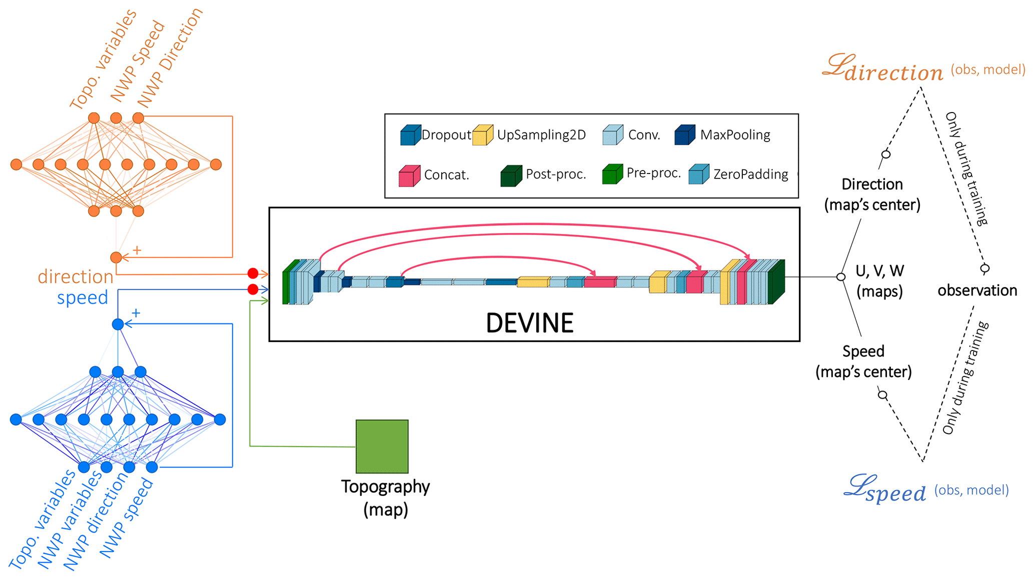
Figure 2Scheme of the new model architecture. The architecture is composed of two artificial neural networks (ANNs) in addition to the DEVINE downscaling model. The first ANN predicts wind direction (orange, ANNdirection), and the second one predicts wind speed (blue, ANNspeed). Skip connections are represented by blue and orange connections associated with the sign “+”. Modified wind speed and direction together with a high-resolution topographic map are then sent to DEVINE (Le Toumelin et al., 2023), which in turn outputs maps of the three components of wind fields (U, V, W) at high resolution (30 m). During the training step, wind direction and speed values are computed at the maps' center (taken to coincide with an observation station) and sequentially compared to in situ observation using appropriate loss functions (see Sect. 3.3.3). ANNdirection and ANNspeed optimizations are guided by the gradient of these losses. We note that ANNdirection and ANNspeed both have an independent model architecture, including the nature of input variables. “Topo. variables” refers to input variables of a topographic nature, “NWP variables” to inputs corresponding to forecasted meteorological and surface variables, “NWP direction” to forecasted wind direction, and “NWP speed” to forecasted wind speed. The mathematical operations performed within DEVINE are listed using colored boxes and are made explicit in Le Toumelin et al. (2023). Finally, red dots following ANNdirection and ANNspeed consist of the intermediate results of the network (i.e., the ANN outputs) and are referred to as Neural Network.
3.3.3 Loss functions
Two loss functions were selected for training ANNdirection and ANNspeed. For ANNdirection we selected the cosine distance (ℒdirection, Eq. 2) to account for angular differences between direction predictions (directionmodel) and observations (directionobs). We also took care to express all the directions in degrees or radians when required.
For ANNspeed we designed a custom loss function that targets the main errors typically found in AROME forecasted wind fields. Previous studies (e.g., Dujardin and Lehning, 2022; Bolibar et al., 2020) demonstrated that the use of a classic loss function (e.g., mean squared error) tends to produce a squeezed distribution around the mean value of the output and poor evaluation metrics. Our loss function, denoted as ℒspeed (Eq. 3), is designed to penalize three specific characteristics of AROME's wind field errors as follows: ℒspeed (i) compares simulated values to actual in situ observations using the mean squared error (mse), (ii) uses the factor τ to foster the correction of speed underestimations over overestimations (τ is arbitrarily fixed to 0.6 for cases of underestimations and 0.4 for overestimations), and (iii) places a higher penalty on errors made at high wind speeds by scaling ℒspeed with observed speeds (speedobs).
3.4 Data partitioning
Deep-learning applications commonly involve the use of a training set for model optimization and a test set for model evaluation. Many studies (Goutham et al., 2021, e.g.,) implement a random train–test split, i.e., randomly extracting test samples from the training set to form a test set. As underlined by Dujardin and Lehning (2022), this method can lead to an overestimation of the model performance. Evaluating a model after random sampling in a temporal context is equivalent to assessing the ability of the model to reconstruct an incomplete time series given the information of all other known time steps. Furthermore, using a random split or a simple temporal split means that the ability of the model to predict in unknown areas is not documented. This can be detrimental for a large number of applications that require downscaled data over areas different from the calibration area. In this study, we decided to evaluate our model both over observational sites not used during training and for a year that was not included during training. This method corresponds to a spatiotemporal extrapolation assessment and provides a strict evaluation procedure closer to real use cases where a model is run over diverse areas largely not present in the training set. Consequently, we divided our dataset into a training set and a test set using a temporal split and a spatial split.
Space partitioning
The spatial split involved a stratified selection process that resulted in the selection of 55 AWS sites from the 273 sites available in the Alps. We first identified six topographic and geographic descriptors for the AWS locations, calculated as described in Sect. 2.3: elevation, the TPI, the slope, the local Laplacian, and the x and y geographical coordinates of the stations (expressed using the Lambert93 projection). For each parameter, we split the 273 AWS sites into three groups according to their position in the parameter's distribution: stations with a parameter below the 0.33 quantile, between the 0.33 and 0.66 quantiles, or above the 0.66 quantile. We then divided each of these three groups into three additional categories according to the root mean square error (RMSE) of AROMEforecast at each site. We applied a random sampling without replacement in the final three groups and ensured that no station was selected twice. Considering the 6 parameters categorized into 3 intermediate groups that are in turn categorized into 3 groups, we identify stations that are representative of diverse topographic parameters, geographic locations, and AROME performances. We also included Col du Lac Blanc station (, ; elevation=2720 m), as it has been studied in Le Toumelin et al. (2023) and we wanted to study our new model at this site. After this spatial split, our training set is composed of the remaining 218 AWS sites and our test set of the 55 selected AWS sites. The stratified selection process favors the selection of a test set that is balanced among the six selected parameters and that has a diverse range of AROME performance, limiting the risk of unbalanced properties of the observational sites among training and test sets.
Time partitioning
The temporal split simply consisted of excluding the last year of data from the training set and excluding the first 2 years from the test set. Finally, we obtain 2 years of data at 218 sites for training and 1 other year at 55 other sites for evaluation.
3.5 Neural network interpretability
3.5.1 Partial dependence plots
In statistical modeling, interpretability methods give insights into the causes that lead a model to make a specific decision. Among these methods, partial dependence plots (PDPs) form an intuitive method giving insights into the isolated effect of a given variable on the model outputs. Their computation consists of iteratively fixing all instances of the studied input variable variablei at a precise value defined in a given range and observing the mean effect on the model outputs. By averaging over all the model outputs, PDPs permit us to focus solely on the influence of variablei on the outputs. PDPs suppose independence between input variables since fixing variablei to a given value comes with no modification of the other input variables. Using PDPs with correlated features can lead to unrealistic situations where model predictions are performed for implausible data instances (e.g., studying the effect of temperatures >20 ∘C over high-altitude stations during winter nights). However, in contrast to accumulated local effects (see Sect. 3.5.2), PDPs do not suppose any ordering in the input variable, in contrast to accumulated local effects (see Sect. 3.5.2). Following this property, we use PDPs in this work to study the impact of ANNdirection input features on wind direction simulations.
3.5.2 Accumulated local effects
Accumulated local effects (ALE) also permit us to study the influence of a given input variable on the model outputs. Unlike more common methods such as PDPs or feature importance ranking (McGovern et al., 2019), ALE are robust to correlated structures in the input variables, which frequently occur in the atmospheric sciences. In contrast to PDPs, ALE compute differences of prediction for a small window around specific values of a given input variable variablei based on its conditional distribution. In detail, this is done by firstly grouping variablei values in n bins of an identical number of instances (quantiles). For each bin, a difference in model predictions is obtained after fixing all instances of variablei to the uppermost value of the bin and subtracting predictions obtained after fixing the same instances to the lowermost values of the bins. This permits us to overcome the correlation issue of PDPs because prediction differences are only computed for data instances in the considered variablei's bin. This step can be interpreted as a computation of a partial derivative around a specific value of variablei. The differences are then averaged to obtain the local effect of variablei for the considered bin. A standard deviation around the mean value is also computed as a way of tracking the dispersion of individual effects. Local effects are then accumulated and centered across each bin to finally obtain ALE. This step corresponds to an integration of the (averaged) local gradients and enables us to represent the dependence of model outputs on variablei across its range. In this study, we also accumulated the standard deviations as a way of keeping track of the dispersion characterizing the individual effects (shaded regions in Fig. 10). Similarly, two-dimensional ALE plots can also be obtained to highlight the effects of the interaction of two features within the model without considering first-order effects. Two-dimensional ALE plots are well suited to observing whether two features interact within the model and help to decompose higher-order causes that lead to model prediction. In this study, ALE are used to understand how input variables of ANNspeed influence Neural Network+DEVINE simulations. More details about ALE can be found in Molnar (2022).
4.1 AROME performance in the Alps
AROMEforecast performances in simulating wind speed in complex terrain depend on the topography. Indeed, we compared AROMEforecast outputs to observed wind speeds in Fig. 3 for a 3-year period at an hourly time step and for all stations available in the Alps (training and test). We then analyzed the influence of topography by grouping observation stations by their quartiles in both TPI500m and elevation distributions. We observe that AROMEforecast is marked by a negative mean bias at both elevated and high TPI500m stations. The joint effect of TPI500m and elevation is all the more marked since speed discrepancies increase with TPI500m for the highest elevation category. In contrast, for lower elevation and TPI500m closer to 0 (i.e., TPI500m in the second and third quartiles), we note a positive speed bias that is less intense than its negative counterpart. Numbers in Fig. 3 indicate the number of observation stations in each group and inform the topographic characteristics of our observational dataset. Notably, we observe that elevated stations are partially correlated with TPI500m (Pearson correlation coefficient = 0.39). High positive values of TPI500m indicate that the observation station dominates its neighborhood and is to some extent “exposed”. TPI500m close to zero characterizes stations on average at the same elevation as their neighborhood in a radius of 500 m, a definition that includes flat terrain.
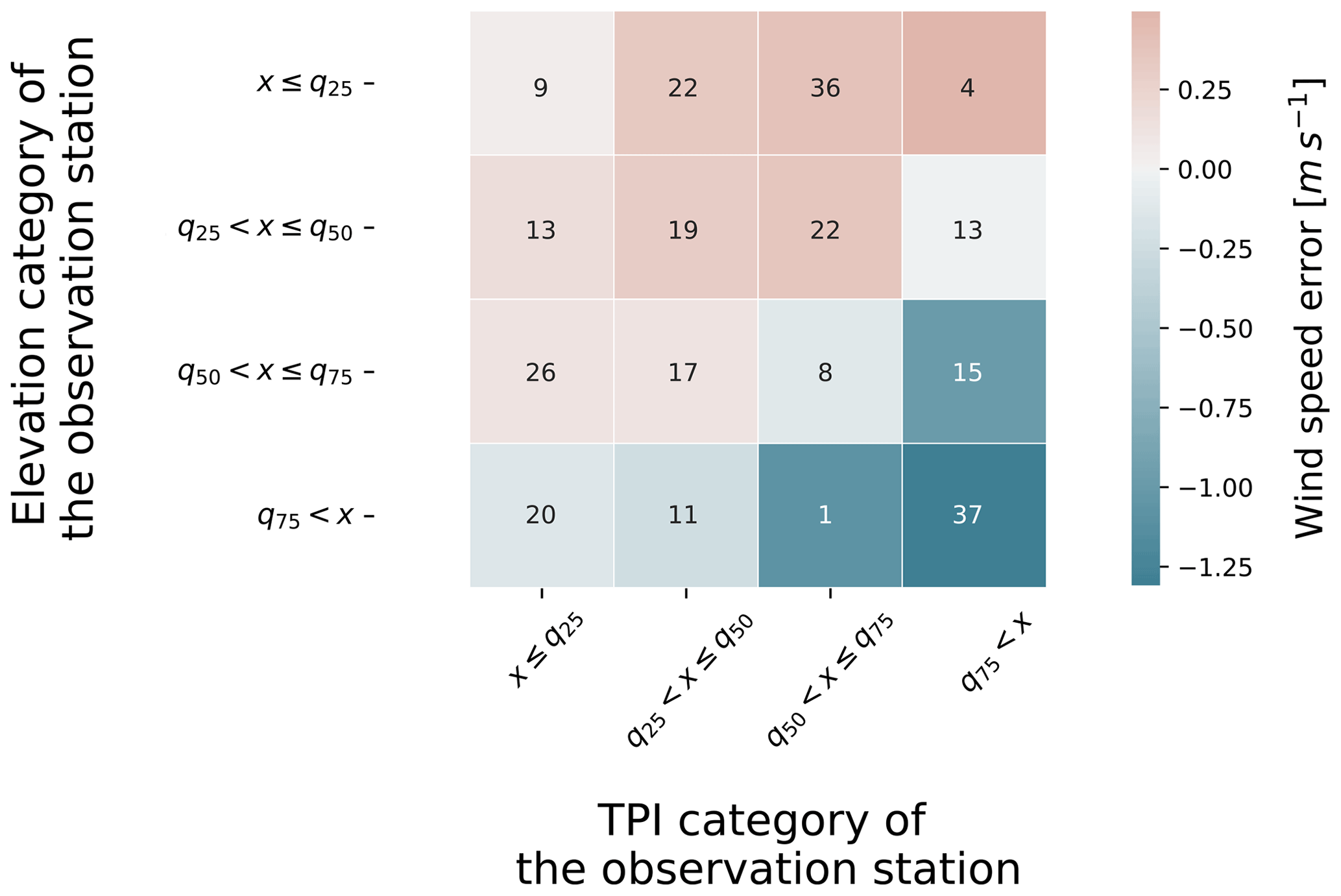
Figure 3Mean wind speed error of AROME forecasts versus observed wind speed (color) at all stations available (training and test) in the Alps. The results are categorized by TPI500m and elevation quartiles (q) at the observation stations. The numbers indicate the number of observation stations within each category. The TPI500m (elevation) values of q25, q50, and q75 are −20, −2, and 11 m (482, 859, and 1605 m).
In addition, we observe that the AROMEforecast negative bias varies with the observed wind speed. Figure 4a compares AROMEforecast hourly simulations to hourly observations and shows the onset of a negative bias with increasing observed speed. This behavior is characterized by a departure from the 1-1 line for the highest observed wind speeds. This observation is consistent with Fig. 3 since, generally, (i) wind speed increases with elevation and (ii) high speeds are generally observed over summits, crests, and ridges (Whiteman, 2000), which designate topographic features often characterized by a high TPI500m. Figure 4 confirms and generalizes the results from Le Toumelin et al. (2023), who already showed this AROMEforecast underestimation pattern in the French Alps: note that the test set used in Fig. 4 shares five observation stations with the Le Toumelin et al. (2023) dataset.
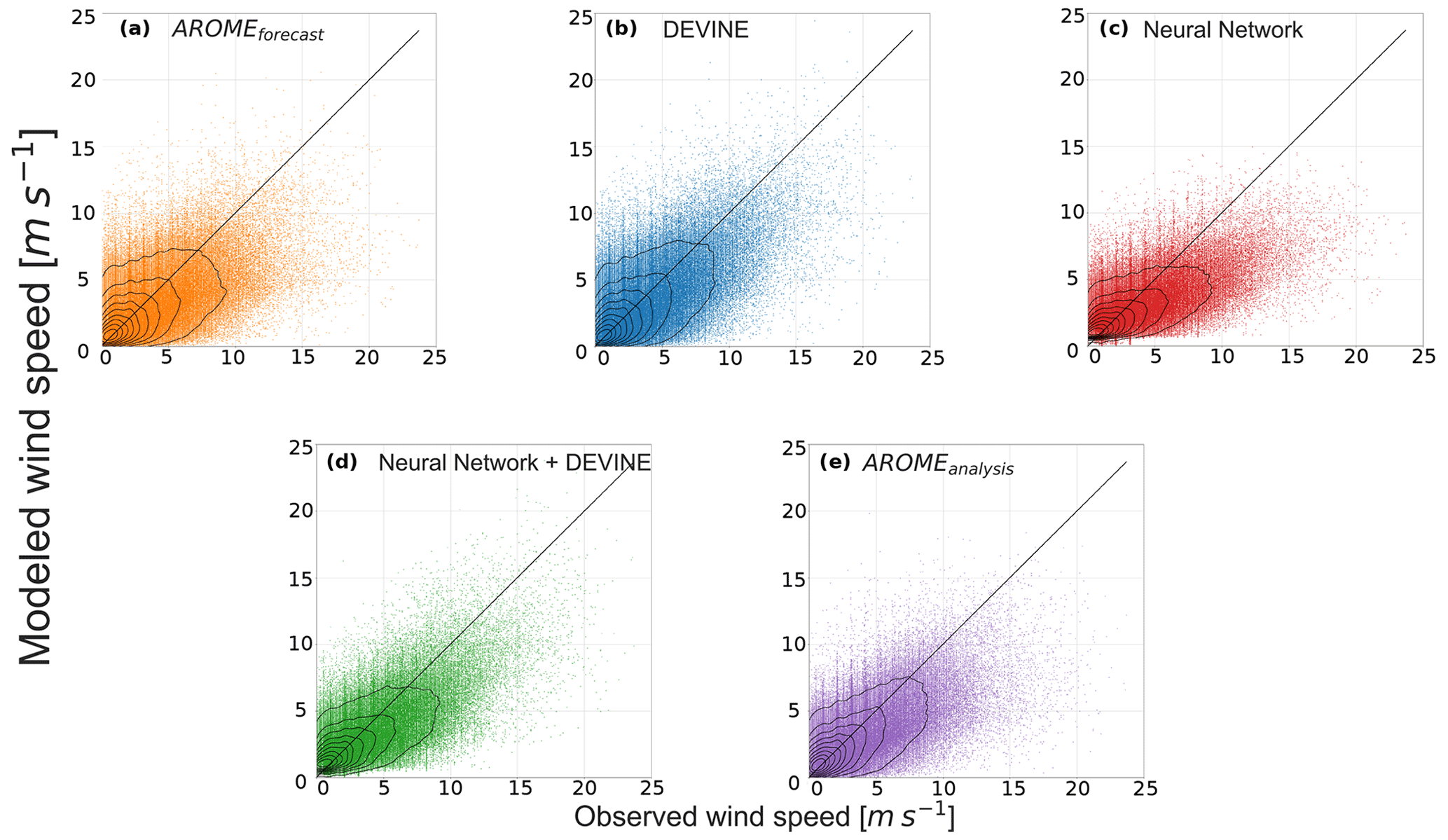
Figure 4The 1-1 plots of simulated versus observed wind speed. The models are (a) AROMEforecast, (b) DEVINE, (c) Neural Network, (d) Neural Network+DEVINE, and (e) AROMEanalysis. Black lines indicate data density. This figure only uses data from the test set.
Finally, AROMEforecast captures realistic wind direction patterns in the Alps. This is qualitatively shown in Fig. 5a and d, where the AROME wind distribution closely resembles the observed wind distribution. We nevertheless observe discrepancies such as a shift in the most frequent wind direction. Indeed, the west-southwesterly wind direction is the most frequent direction among our observations, whereas AROMEforecast predominantly simulates southwesterly wind fields. For all the directions, we note that most wind direction errors are less than 60∘ and less than 30∘ when forecasted among the dominant directions (west-southwest and southwest). The largest direction errors (i.e., errors greater than 90∘) affect all the directions in comparable proportions. We finally observe that AROMEforecast tends to overestimate the west-northwesterly, northwesterly, and north-northwesterly directions while underestimating the northerly direction.
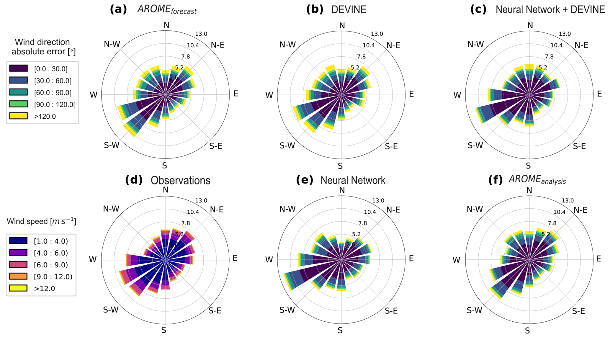
Figure 5Wind roses of modeled wind directions for (a) AROMEforecast, (b) DEVINE, (c) Neural Network+DEVINE, (e) Neural Network, (f) AROMEanalysis, and (d) observed wind directions. Colors in panels (a–c, e, and f) indicate the wind direction modeling error, obtained by comparing modeled and observed wind directions. Colors in panel (d) indicate the speed category of the observed wind. Only wind directions acquired for observed and modeled wind speeds above 1 m s−1 have been considered. The spoke on the radial axis indicates the proportion in the percentage of data that is predicted in the considered direction.
4.2 Model evaluations
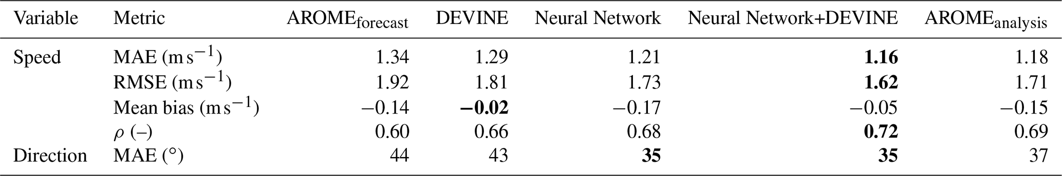
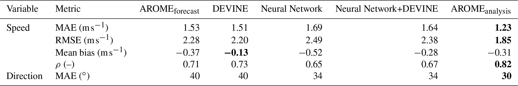
In this section, we evaluate the performances of different wind products, including AROMEforecast and AROMEanalysis, as well as the results of our deep-learning corrections and/or downscaling models (DEVINE, Neural Network, and Neural Network+DEVINE). Consequently, we use the test dataset, which was not used to train the deep-learning models. We remind the reader that AROMEforecast serves as input for DEVINE and Neural Network+DEVINE, while both deep-learning models did not use directly any data from AROMEanalysis as input. Integrated evaluation metrics first highlight an improved RMSE, MAE (mean absolute error), mean bias, and coefficient correlation with DEVINE over AROMEforecast (Table 3). Such improvements are not able to bridge the gap between AROMEforecast and AROMEanalysis, the latest showing largely improved evaluation metrics. However, the use of Neural Network+DEVINE improves statistics (except mean bias), ultimately showing the best results among all the wind products.
We also observe (as expected) improved behavior of AROMEanalysis over AROMEforecast, notably through a partial correction of the departure from the 1-1 line for high observed speeds initially observed in AROMEforecast (Fig. 4). More generally, AROMEanalysis data are centered around the 1–1 line, suggesting better agreement between simulations and observations. Similarly, we observe that DEVINE generates increased wind speed, notably for the highest observed speeds. Such a modification compensates for the AROMEforecast initial underestimation. However, contour lines which indicate data density still reveal some dispersion around the 1-1 line with DEVINE. Neural Network+DEVINE also shows a partial correction for the highest observed speeds and shows generally less dispersion around the 1-1 line. A close inspection of the lowest wind speeds however indicates some overestimation of null speeds and speeds less than 1 m s−1.
Table 3Evaluation metrics obtained on the test dataset (Alps). MAE designates the mean absolute error, RMSE the root mean square error, and ρ the Pearson correlation coefficient. The mean absolute error for wind direction was computed by taking into account the cyclic nature of wind direction. The best metrics are shown in bold font.
We then scrutinized the model performances for wind speed with respect to elevation in Fig. 6a. DEVINE performances are comparable to AROMEforecast performances for low-elevation stations, in addition to the fact that, in contrast to AROMEforecast, DEVINE provides a spatialized signal at a local scale. Improvements are however observed for higher stations and can be attributed to the ability of DEVINE to simulate acceleration at exposed and elevated stations where AROMEforecast denotes a negative bias compared to observations. These results reinforce a study with DEVINE (Le Toumelin et al., 2023) that observed similar behaviors. AROMEanalysis presents better evaluation metrics compared to AROMEforecast and DEVINE in all the elevation categories. However, we still observe some errors at the most elevated stations. Neural Network+DEVINE finally improves DEVINE evaluation metrics in all the elevation categories, matching AROMEanalysis metrics on the second and third quartiles and outperforming them for the most elevated stations. In detail, the boxplot indicates slightly lower median errors for AROMEanalysis compared to Neural Network+DEVINE in all the categories except for the highest stations but also shows that the largest modeling errors are less frequent with Neural Network+DEVINE among the third and fourth quartiles.
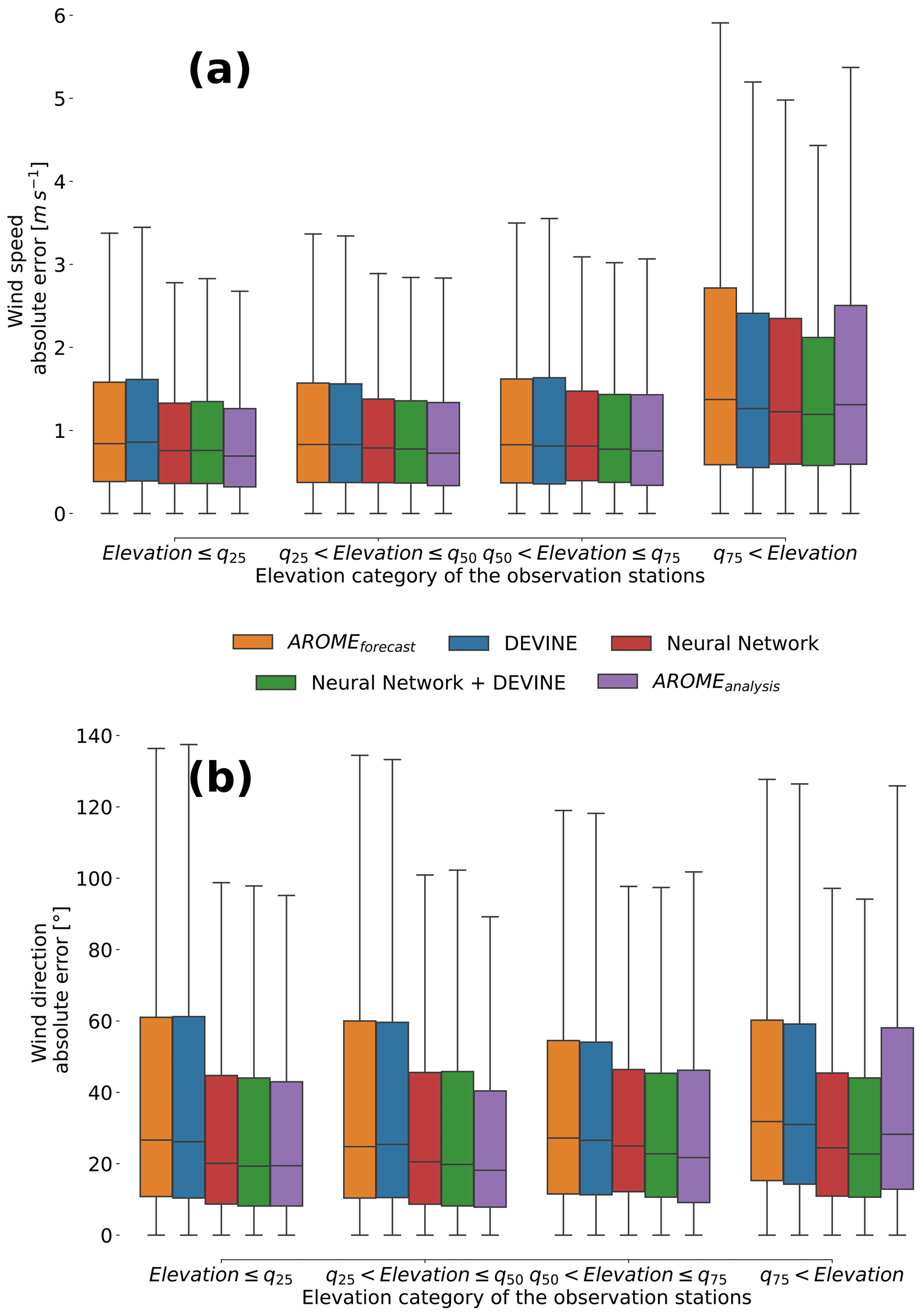
Figure 6Wind direction absolute error (a) and wind speed absolute error (b) categorized by the elevation of the observation station where the measurements were taken. In detail, the four categories correspond to the four quartiles of the elevation distribution among the observation stations: elevation increases from left to right. Each boxplot color indicates a different model. This figure only uses data from the test set.
In terms of wind direction, AROMEanalysis largely decreases the largest modeling errors observed in AROMEforecast. Wind distribution patterns highlight a reinforcement of the occurrence of wind in the southwesterly direction, which is still different from the observed wind patterns (Fig. 5). However, we see improvement in the reduction of north-northwesterly predictions and better characteristics concerning the northerly to easterly winds. On the other hand, as noted in Le Toumelin et al. (2023), DEVINE simulates directions close to AROMEforecast without introducing any major change. Similarly to observations, Neural Network+DEVINE simulates most winds in the west-southwesterly direction and largely reduces the occurrence of the largest wind direction errors (Fig. 5). The improved performance is striking in the dominant westerly directions. Figure 6b sheds light on the distribution of errors according to the elevation category of the observation stations and shows similar characteristics to speed errors. Similarly to AROMEanalysis, Neural Network+DEVINE improves wind direction modeling over AROMEforecast and DEVINE in all the elevation categories, notably at the most elevated stations where Neural Network+DEVINE has the lowermost median value for direction errors among all the products compared.
4.3 Influence of forecast lead time and seasonality
In this section, we analyze model performances with respect to forecast lead times (Fig. 7a and c) and month of the year (Fig. 7b and d). We note that, in our study, a forecast lead time has a one-to-one relationship with the hour of the day. In terms of speed, AROMEforecast errors are characterized by a peak occurring for lead times between 10 and 20 h, i.e., mostly during midday and afternoons, in phase with the daily peak of the average wind speed. This peak vanishes with AROMEanalysis, which shows considerable improvements compared to the forecasts. Moreover, we observe that DEVINE shows small yet notable improvements compared to AROMEforecast. Neural Network shows general improvements compared to AROMEforecast and DEVINE by shifting down the error curve but still preserves a peak around lead time 15 h. Finally, the use of DEVINE after Neural Network (Neural Network+DEVINE) again diminishes the mean error in a manner quite similar to the use of DEVINE after AROMEforecast. Ultimately, we observe that mean errors are lower with Neural Network+DEVINE than with AROMEanalysis for the longest (>18 h) and shortest (<8 h) lead times.
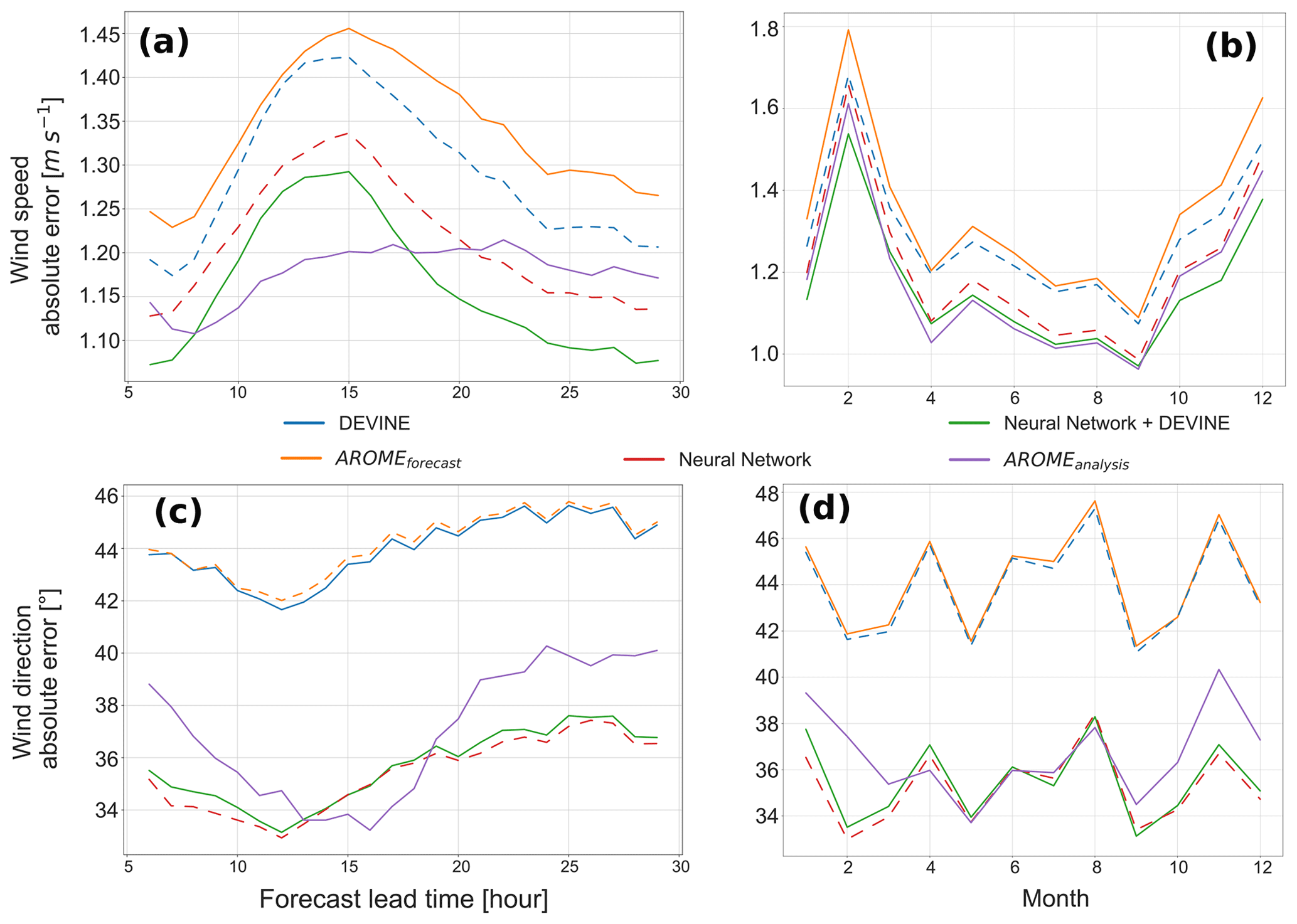
Figure 7Wind speed absolute error as a function of the forecast lead time (a) and month of the year (b). Wind direction absolute error as a function of the forecast lead time (c) and month of the year (d). Colors indicate the different models. This figure only uses data from the test set.
We obtain similar model rankings in terms of wind direction. Nevertheless, we observe that the AROMEforecast direction error is marked by a minimum around 12 h, which is interestingly shifted from the maximum in the speed error observed at 15 h. This minimum is shifted by 1 h, is intensified in AROMEanalysis, and is not modified in Neural Network or Neural Network+DEVINE. The modifications added by DEVINE to the evaluation metrics are low in terms of direction. However, a clear diminution of the error is observed when using Neural Network and Neural Network+DEVINE, which underlines the added value of Neural Network, far more than DEVINE, in terms of directional predictions. Similarly to speed predictions, the best statistics among all the products are obtained with Neural Network+DEVINE over the largest part of the day, especially for the lowermost and uppermost lead times, when it outperforms AROMEanalysis.
When modeling errors are interpreted with regards to the month of the year, we observe a peak in speed error during the winter months (Fig. 7b and d). This observation is consistent with the fact that, in mountainous terrain, the highest wind speeds often occur in winter (Kruyt et al., 2017). Model intercomparison highlights a similar ordering between models to that which happens at the daily scale. The use of Neural Network notably decreases the error curve. Ultimately, Neural Network+DEVINE compares well with AROMEanalysis, notably during the winter months, when it outperforms it. In contrast to wind speeds, wind direction errors do not show any dependence on seasonality. Model ordering is however comparable to the ordering concerning speed metrics, with the difference that the use of DEVINE does not show any improvements in terms of aggregated metrics. Again, Neural Network+DEVINE permits us to reduce wind modeling error, with a reduction leading to lower errors in winter compared to AROMEanalysis.
4.4 Influence of the loss function
The design of an appropriate loss function was important for ultimately obtaining the best-performing model presented in this study. The function used to optimize ANNspeed (ℒspeed) permits us to obtain better integrated metrics (MAE, RMSE, and Pearson correlation coefficient) and to capture a wind speed distribution closer to the observed speed distribution. As demonstrated in Fig. 8, which compares observed speed quantiles to simulated quantiles, the use of ℒspeed shortens the gap between AROMEforecast quantiles and the 1-1 line. When fitting the ANNspeed with a classical MSE loss function, we obtain a speed distribution with Neural Network+DEVINE which overestimates low quantiles and underestimates high quantiles, i.e., has a tendency to squeeze results around a mean value as already observed by Dujardin and Lehning (2022) for similar applications. The improvements observed after using ℒspeed are most notable for high wind speed, which is consistent with the different terms comprising ℒspeed (see Sect. 3.3.3). This however contrasts with a degradation of the simulation of very low wind speeds: emphasizing the correction of high wind speeds comes at the cost of putting less penalty on lower wind speeds and hence results in a model that performs worse concerning the first speed quantiles. The use of MSE in place of ℒspeed to optimize ANNspeed also deteriorates integrated metrics, illustrated by a 12 % increase in MAE on the test set. We did not design a custom loss function for direction but simply selected ℒdirection (Eq. 2), which immediately yielded satisfactory results.
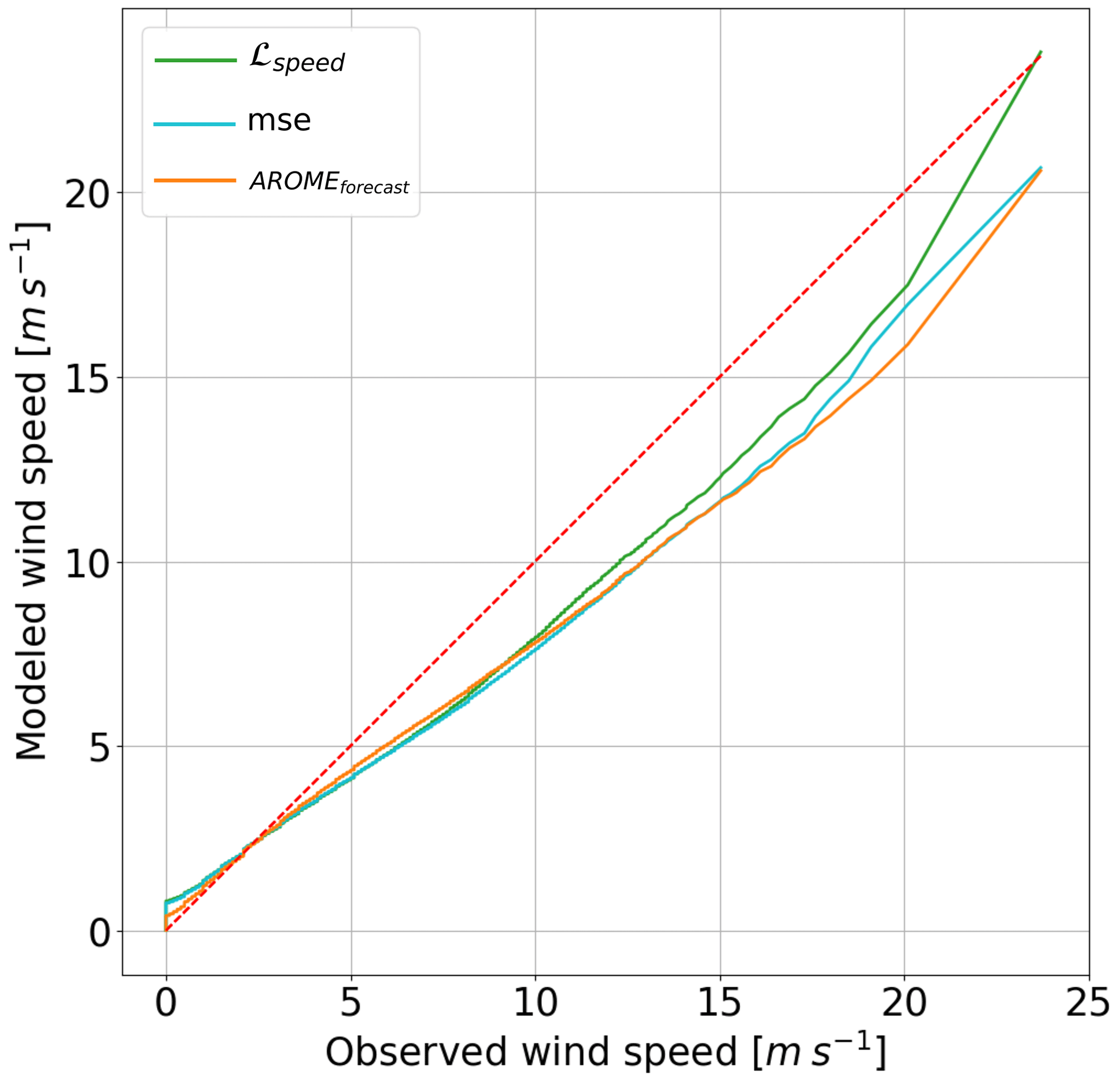
Figure 8Plot of the observed quantiles versus the modeled quantiles for different models. A perfect simulation would present all quantiles along the 1-1 line (red). Each color refers to a single model, mse refers to Neural Network+DEVINE optimized using a mean square error loss function, and ℒspeed refers to the reference simulation, i.e., Neural Network+DEVINE optimized using ℒspeed (Eq. 3). This figure only uses data from the test set.
4.5 Sensitivity to the geographical situation
When fitted using observation from the Alps, Neural Network+DEVINE yields poor evaluation metrics in terms of speed when evaluated against data from other mountain ranges but performs well when downscaling wind direction. We evaluate the ability of our models to correct and downscale AROMEforecast over 18 AWSs in Corsica and 21 AWSs in the Pyrenees, which are both located hundreds of kilometers from the Alps and are exposed to different weather regimes. Data from these ranges were not used during training. In Corsica and the Pyrenees, Neural Network+DEVINE systematically degrades the RMSE, MAE, and Pearson correlation coefficient for wind speed when compared to AROMEforecast and AROMEanalysis (Table 4). As an illustration, the RMSE increases by 7 % with Neural Network+DEVINE compared to AROMEforecast. In contrast, we observe that DEVINE alone improves AROMEforecast metrics in a manner similar to the evaluation performed in the Alps (Table 3). Surprisingly, the evaluation of wind direction highlights the improvement with Neural Network+DEVINE with respect to AROMEforecast (MAE is reduced by 6∘), whereas DEVINE again does not influence the mean wind direction. Wind directions from Neural Network+DEVINE are however on average less precise than with AROMEanalysis, in contrast to the Alpine situation. We can hypothesize that, since ANNdirection input variables include almost only variables of a topographic nature, corrections added by ANNdirection are more linked to local topography than to meteorological situations and hence better generalize to other mountain ranges. This exploration of the extrapolation abilities of our models to other mountain ranges points towards the need for additional training if the models are to target areas outside the western (French and Swiss) Alps. It does however confirm the generic character of DEVINE as already highlighted in Le Toumelin et al. (2023), which does not require any further calibration to be applied to a diversity of Alpine-type mountain ranges.
Table 4Evaluation metrics obtained by comparing simulation and observed data in other mountain ranges (Corsica and the Pyrenees) than the one used during training (Alps). No data from Corsica (18 AWSs) or the Pyrenees (21 AWSs) were used during training. MAE designates the mean absolute error, RMSE the root mean square error, and ρ the Pearson correlation coefficient. The mean absolute error for wind direction was computed by taking into account the cyclic nature of wind direction. The best metrics are shown in bold font.
4.6 Case study
To illustrate the added value of Neural Network+DEVINE compared to DEVINE alone, we selected a case study at a mountain observation station located near Piz Corvatsch in southwestern Switzerland (latitude=46.41, longitude=9.82; elevation=3294 m). On 8 October 2019 at 06:00 UTC, AROMEforecast simulates calm wind conditions (1 m s−1) for a wind coming from the southwest (242∘). DEVINE downscales the large-scale wind field of AROMEforecast to a local scale. As a result, it increases AROMEforecast wind speed to 1.47 m s−1 in the close vicinity of the location of the AWSs, since the site is localized on a ridge prone to wind acceleration (Fig. 9). In contrast to both AROMEforecast and DEVINE, the observation indicates a wind coming from the northwest (329∘) and a much higher speed (6.4 m s−1), which is also partially captured by AROMEanalysis and indicates a direction of 293∘ and a speed of 1.81 m s−1. This example sheds light on high discrepancies than can affect DEVINE input variables (5.4 m s−1 speed error, 87∘ direction error). In contrast, Neural Network modifies the AROMEforecast wind direction by introducing a 80∘ clockwise direction change, which puts the direction closer to the observations. Similarly, Neural Network multiplies the speed by a factor of 2.6, ultimately reaching a value of 2.7 m s−1. After Neural Network, DEVINE downscales these modified large-scale conditions. As typically observed with DEVINE, modifications in wind directions are modest. However, the speed reaches 3.02 m s−1, reducing the initial error by 31 %. Since the optimization of Neural Network has been obtained after back-propagating error gradients through both DEVINE and ANNs, we can expect that the deep-learning model is to some extent aware of the expected effect of DEVINE and prevents it from overcorrecting AROMEforecast. By scrutinizing the day before and after this specific meteorological situation, we observe that AROMEforecast systematically underestimated wind speed at this specific location, which is partially corrected by Neural Network+DEVINE. However, this model chain is also responsible for lowering the speed's temporal variability, which was already too low with AROMEforecast. During this period, the direction shifts from a northeasterly direction to a westerly direction. The largest modeling errors are observed during the transition period, when Neural Network+DEVINE contributes to bridging the gaps to observations. During the final hours, AROMEforecast captures a more correct wind direction at the station, and the added value of Neural Network+DEVINE is lower. Neural Network+DEVINE however still keeps its ability to spatialize the wind signal over the study area, which is necessary for many applications that require high-resolution forcings in complex terrain.
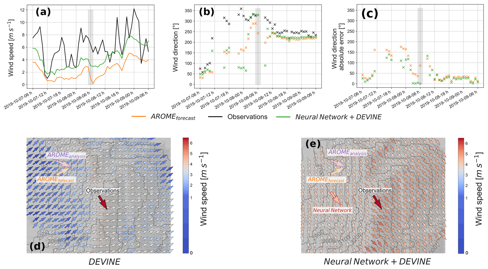
Figure 9Use case of Neural Network+DEVINE at Piz Corvatsch in Switzerland for 7 to 9 October 2019. Panel (a) presents a time series of observed and simulated wind speeds, panel (b) presents observed and simulated wind directions, and panel (c) shows the modeling errors in the wind direction. Panel (d) represents a two-dimensional view of the wind map around the station for 8 October 2019 at 06:00 UTC. This date corresponds to the shaded areas in panels (a–c). Small arrows were obtained using DEVINE, fed by AROMEforecast. Panel (e) was similarly obtained but using Neural Network+DEVINE. AROMEanalysis and Neural Network (the intermediate result) are shown for interpretation. Colors inside arrows indicate wind speed: red colors indicate speeds larger than AROMEforecast and blue arrows the opposite. The geographical position of AROMEforecast corresponds to the location of the nearest grid cell from the observation station in the AROME grid. AROMEanalysis and Neural Network are located at the same position but were moved to the close vicinity of AROMEforecast for visual purposes. The high-resolution arrows in panels (d) and (e) correspond to the downscaled signals by DEVINE and Neural Network+DEVINE characterized by a lower grid spacing than the other wind products; these arrows were initially distant from 30 m and have been downsampled to 90 m for visual purposes. The location (Piz Corvatsch) and times (7 to 9 October 2019) are only found in the test set.
5.1 Performances and modularity of the chosen architecture
Neural Network+DEVINE shows improved metrics when compared to AROMEforecast and DEVINE in terms of both speed and direction. This is highlighted by more accurate 1-1 plots for wind speed (Fig. 4), better wind distributions (Fig. 5), lower speed and direction errors when errors are categorized by elevation (Fig. 6), forecast lead time or month (Fig. 7), and improvements in the integrated metrics (RMSE, MAE, and correlation coefficient, Table 3). Evaluation metrics obtained with Neural Network+DEVINE sometimes overpass metrics obtained with AROMEanalysis, e.g., at elevated stations or during the winter months, suggesting that our method introduces notable added values when compared to other well-known atmospheric products. Even though comparisons between Neural Network+DEVINE and AROMEanalysis are limited by a scale discrepancy, supplementary analysis shows that the comparison still holds when AROMEanalysis is downscaled to a 30 m horizontal grid spacing with DEVINE (Fig. S1 in the Supplement). Improved evaluation metrics are all the more encouraging as metrics have been obtained using a spatiotemporal extrapolation assessment, i.e., testing the model at locations not included in the training set and for a year not included either. This corresponds to a very strict evaluation procedure, which makes it generally harder to obtain good evaluation metrics versus simpler evaluation procedures that only perform tests at the sites included in the training set (Bolibar et al., 2020; Dujardin and Lehning, 2022).
The modular architecture of Neural Network+DEVINE appears to us to be one of its greatest assets. Decoupling the spatial interpolation of wind fields (in DEVINE) from its correction (in Neural Network) makes the model robust to new NWP systems or NWP version evolutions. Indeed, if a new version of AROMEforecast were to be released with important changes, possibly breaking the learned relationships between input variables and observed wind, our architecture permits us to simply bypass Neural Network and rely on DEVINE while a new fit is performed with the new NWP version. The same reflection applies to the use of Neural Network+DEVINE at other mountain ranges. As demonstrated in Sect. 4.5, the full model chain is not directly operable on mountain ranges where no data were used during training. As a consequence, a training step is required to adapt Neural Network weights and biases to learn geographically variable relationships between inputs and targets (mostly for ANNspeed). In the meantime, and in contrast to more classical models that perform model output statistics, the user could rely on the standalone use of DEVINE, which showed good generalization capabilities in other Alpine-type mountain ranges. Conversely, if user applications that require high-resolution wind forcing are not only dependent on the spatial structure of the signal but also require a high degree of plausibility of the downscaled values, the integration of a training phase in the pipeline is possible and would lead to an optimized version of the downscaling scheme. This flexibility does not exist in downscaling methods that do not incorporate any fit to observed data.
Since we did not modify the DEVINE downscaling model in this study but only added upstream modifications related to coarse-scale wind fields, our new architecture inherits the pros and cons of the downscaling model concerning the local structures of simulated wind fields. On the one hand, using DEVINE favors the simulation of spatially consistent three-dimensional outputs at a local scale since DEVINE was built to replicate the structure of outputs provided by an atmospheric model (Helbig et al., 2017). On the other hand, DEVINE limitations persist, which is illustrated for instance by the absence of local-scale turbulent structure in the wind outputs (Le Toumelin et al., 2023).
In addition to potential applications in wildfire spread modeling, wind energy forecast, wind energy potential assessment, pollutant dispersion evaluation, drifting-snow modeling, and avalanche hazard forecasting (Giovannini et al., 2020; Wagenbrenner et al., 2016; Dujardin and Lehning, 2022; Lehning and Fierz, 2008), other applications are sensitive to the accuracy of wind forcing in mountainous terrain. For instance, meteorological forecasters rely on accurate wind predictions in mountains for weather nowcasting and short-term forecasting: they could benefit from the use of a high-resolution product such as Neural Network+DEVINE since the modeling chain yields improved wind values when compared to other products (e.g., AROMEforecast and AROMEanalysis) under specific topographic and weather situations. Other examples are the use of physics-based models for research purposes in past and future trends in water availability, glacier evolution, and more generally environmental changes. These models often require meteorological information such as wind speed at various scales of interest, including the hectometric scale. For instance, Réveillet et al. (2018) showed the importance of correctly simulating wind speed in order to simulate the mass balance of a medium-sized Alpine glacier when using an energy-balance model, an issue that concerns past simulations as much as future projections. Since input variables used in Neural Network are standard NWP output and topographic indicators derivable from DEMs, we hypothesize that Neural Network could be trained by using reanalyses (e.g., SAFRAN, Vernay et al., 2022; ERA5, Hersbach et al., 2020). On top of a capability to downscale reanalysis wind fields in the past, this could also enable us to downscale the wind of climate projections bias-corrected against these reanalyses, e.g., the ADAMONT projections (Verfaillie et al., 2017) widely used in France.
5.2 Neural network explainability
ANNspeed input features have various, unequal, and nonlinear contributions to Neural Network+DEVINE outputs (Fig. 10), as estimated using ALE (see Sect. 3.5.2). In summary, ALE determine the effect of each input variable on the average output, conditional on the values of an input feature. The most prominent effects are observed for the Wind Speed10m input feature (Fig. 10p), which confirms our expectations since it corresponds to the downscaled variable modified in ANNspeed output. The use of a skip connection (Fig. 2) for this variable may also play a role in maintaining it as the most important variable for downscaling even though correlated variables, such as wind speed at other atmospheric levels, are also used as inputs. Wind speed computed by AROMEforecast at other atmospheric levels shows strong effects on the outputs, most notably when it concerns high speed values.
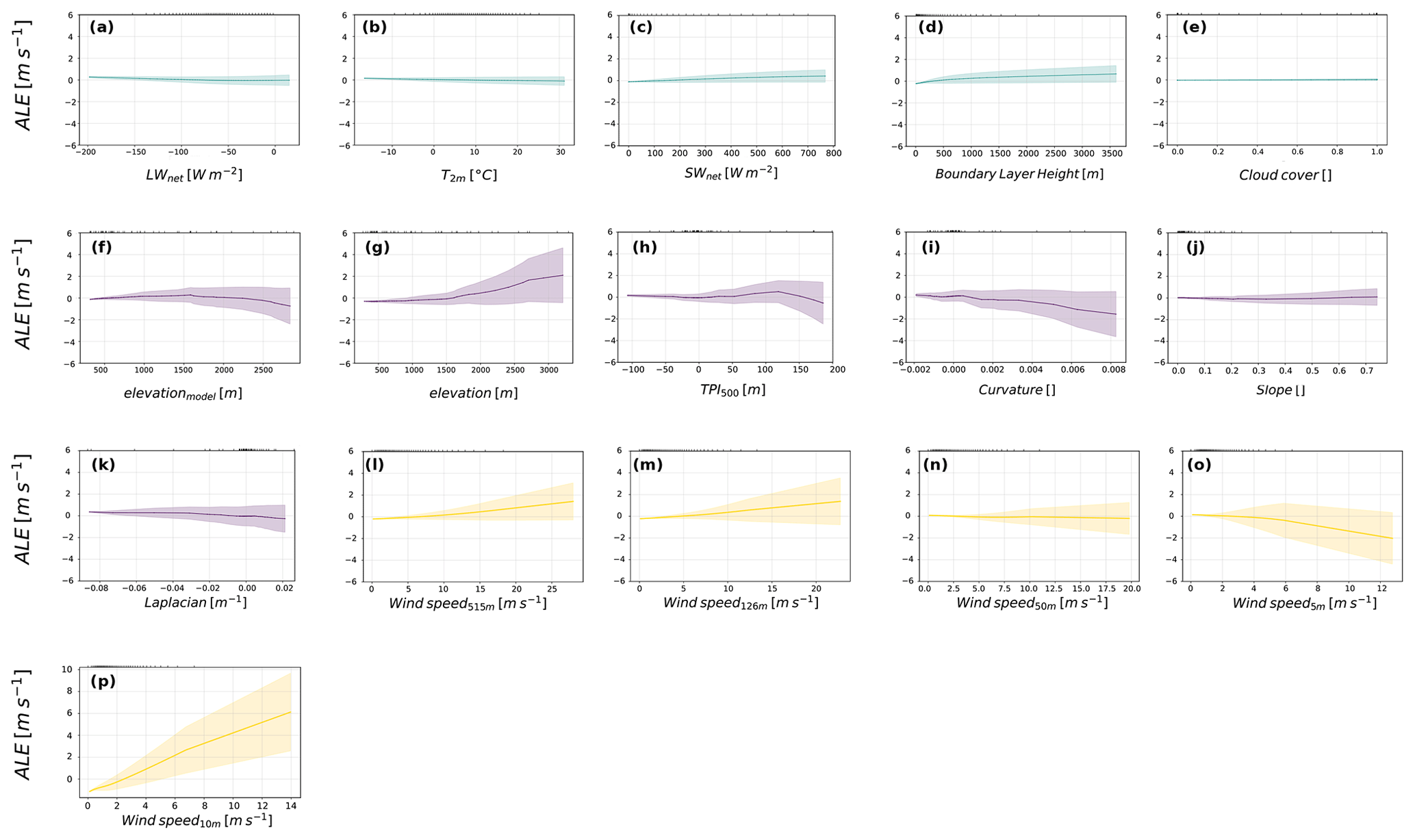
Figure 10Accumulated local effects (ALE) associated with each input variable of ANNspeed (solid lines). ALE are expressed in meters per second and can be interpreted as the effect of a specific variable at a certain value compared to an average prediction. Shaded areas indicate cumulative dispersion around the mean local effects and increase in each panel from left to right by design. Variations in shaded areas indicate additional uncertainty, and comparisons of shaded areas across the panels give insights into uncertainty differences in ALE computation. The small ticks at the top of each panel represent distribution quantiles that were used to compute ALE. Green, violet, and yellow colors indicate, respectively, input meteorological variables, topographic variables, and wind-related variables.
Topographic parameters also have strong impacts on the speed outputs, particularly when this concerns the tails of the parameter distributions. Real elevation (elevation, Fig. 10g) and model elevation (elevationmodel, Fig. 10f) have opposite effects: the first one tends to be positively correlated with speed outputs, and the second one presents a negative correlation. Two-dimensional ALE plots (not shown) suggest almost no second-order interaction between either variable. The joint effect of these variables, approximated by the sum of the first- and second-order effects, suggests increasing speed outputs with increasing elevation. This confirms our initial interpretation of AROMEforecast biases (see Sect. 4.1) that highlighted an average underestimation of speed by AROMEforecast over elevated regions. Interestingly, TPI500m, which was also a variable we identified to possibly account for AROMEforecast biases, presents diverse effects on the outputs. As Neural Network+DEVINE was trained after comparing observed values to downscaled simulations, the effects in Fig. 10 not only compensate for biases in AROMEforecast, but can also relate to local-scale effects in the downscaling module, i.e., counterbalancing missing or incorrectly represented local processes in DEVINE.
Finally, we observe that input variables related to the state of the atmosphere (green-shaded areas in Fig. 10) have a lower influence on the output and tend to be less dispersed. Interestingly, we see that net shortwave radiations at the surface (SWnet, Fig. 10c) increase the speed outputs. This supports Le Toumelin et al. (2023), who observed speed underestimation with AROMEforecast during the afternoons of the summer months, where SWnet is generally high. In contrast, net longwave radiations (LWnet, Fig. 10a), 2 m temperature (T2m, Fig. 10b), cloud cover (Fig. 10e), and local slope (Fig. 10j) show a very modest influence on the outputs. Removing iteratively slope and cloud cover from the input features (which are the less impactful input variables according to ALE) and re-training the model did not impact the evaluation metrics. However, removing all variables with low ALE (LWnet, T2m, cloud cover, and slope) starts to show modifications in evaluation metrics, with for instance the correlation coefficient dropping from 0.72 to 0.70. This could be due to (i) feature interactions not observed in one-dimensional ALE plots, (ii) some unexpected overfitting of the test set, and (iii) the visualization artifact from Fig. 10. Indeed, Fig. 10 highlights the largest effects on the outputs, making ALE close to 1 m s−1 look negligible. However, we remind the reader that 1 m s−1 almost accounts for 50 % of the mean speed value (2.23 m s−1 in AROMEforecast).
Here, ALE appear to be useful for model interpretation and as a tool for input variable selection. Indeed, we can distinguish between three groups of input features of unequal importance within the model (topographic variables, wind-related variables, and other weather-related variables). This is partly supported by additional sensitivity tests that reveal a larger increase in the RMSE when removing the topographic variables (RMSE=1.68 m s−1 versus 1.62 m s−1 with all variables included) or the wind-related variables with the exception of Wind speed10m (RMSE=1.67 m s−1) from ANNspeed input features than when removing other meteorological variables (RMSE=1.65 m s−1).
This is of interest for the application of the Neural Network+DEVINE correction and downscaling strategy to a variety of products like reanalyses, as solely topographic or topographic plus basic atmospheric variables may be easier to access, retrieve, and process than a complex suite of ancillary weather variables not always available in the reanalysis archives.
Input variables of ANNdirection present scattered individual effects probably showing large interactions among input variables within the model when computing the output, as visible in PDPs (Fig. 11). Before using PDPs for ANNdirection, we confirmed that the input variables were not correlated with each other by checking Pearson correlation coefficients. We studied the impact of input features on the directional difference added to the NWP direction on the final ANNdirection output neuron rather than on the value of the downscaled wind direction, as a classic mean value is not defined for cyclic variables such as wind direction. Note that the modifications computed by ANNdirection also take into account DEVINE effects, which are modest concerning wind direction and which can eventually influence model interpretation. Wind Speed10m does not modify the mean direction, which was expected. The mean effect for wind direction fluctuates around 0, which suggests some small adjustment given certain azimuths. The mean effect of aspect is also close to 0, except around 50 and 100∘. The three aforementioned variables were not expected to have a mean effect, which is arguably confirmed by the PDPs. However, interactions among the variables could be anticipated, which is also suggested by the large dispersions around the mean effects. In contrast, α has a strong effect for negative values, which was intuitively expected since this variable already incorporates some interaction between wind direction and aspect. Surprisingly, we do not observe the same behavior for positive α. We remind the reader that the highest absolute values for α are obtained when a flow arrives perpendicularly to a steep vertical slope. The large dispersion around each PDP mean value suggests different scenarios and large variable interactions. Finally, we underline the fact that interpretability methods are important not only for understanding how a model deals with inputs and for feature selection, but also for anticipating model output modifications linked to future evolutions of the model providing input data (here AROMEforecast). As discussed in the previous section, NWP is under constant evolution, frequently incorporating new or modified parameterizations that tend to modify the model's general behavior and affect several atmospheric variables. Interpretability methods such as in Fig. 10 permit us to approximate typical effects that can be obtained through the correction and downscaling model and to anticipate the upcoming possible modeling errors following NWP updates.
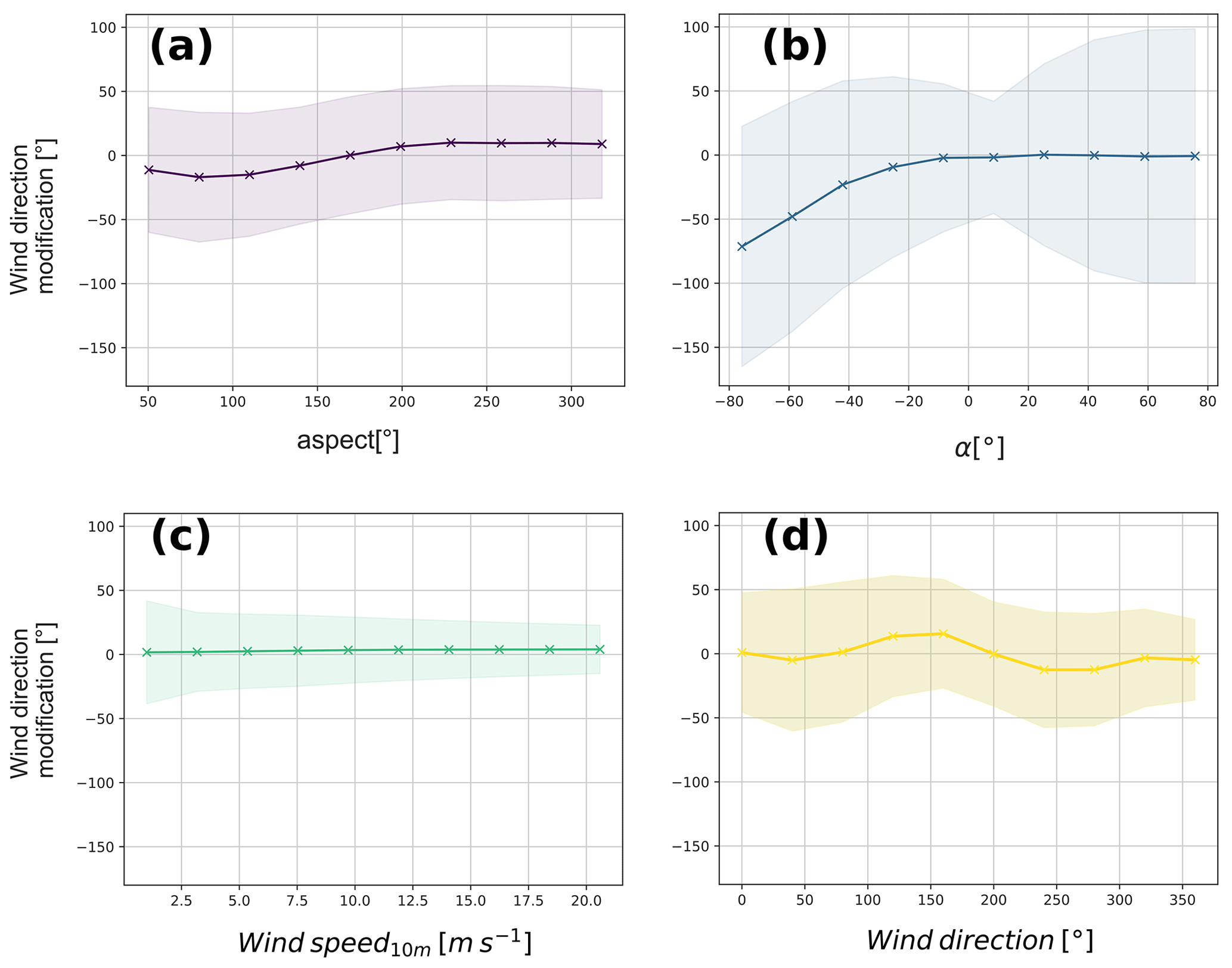
Figure 11Partial dependence plot (PDP) for each input variable of ANNdirection. PDPs represent the mean prediction value obtained after fixing all instances of a specific input variable to a certain value. Shaded areas indicate 1 standard deviation around the mean effect.
Understanding the complex patterns that characterize wind in mountainous terrain is of great importance for several applications, with direct consequences for the environment and human societies. Despite years of continuous improvements, NWP models still rely on downscaling techniques to represent wind features at a local scale in mountains. Not only does the typical kilometer-scale spatial resolution limit their use for several applications, but NWP models are also affected by systematic errors linked to typical meteorological or topographic situations. In this study, we used a large network of observation stations to identify and understand AROMEforecast systematic errors. We observed a strong link between model biases and topographic parameters (a joint effect of elevation and TPI500m) as well as a tendency to underestimate the highest observed speeds.
Aware of the aforementioned limits, here we designed a new postprocessing architecture, called Neural Network+DEVINE, with the purposes of both correcting AROMEforecast errors (i.e., applying model output statistics) and increasing the spatial resolution of the wind signal (i.e., downscaling). This new combined architecture benefits from the use of two artificial neural networks to sequentially correct the coarse-scale wind signal for direction and speed according to specific meteorological and topographic situations before using the statistical downscaling model DEVINE for the spatial interpolation of the wind fields.
This hybrid architecture yields better integrated metrics (MAE, RMSE, mean bias, and correlation coefficient) compared to previous alternatives. The evaluation metrics show performances similar to AROMEanalysis, a system benefiting from assimilation techniques to estimate the most plausible state of the atmosphere in complex terrain. Notably, most improvements are obtained at elevated and exposed stations during winter months and more generally for simulating the largest observed speeds, which suggests that our new method is well tailored for drifting-snow applications.
This new type of downscaling model greatly benefits from its modular architecture on several points. By making a distinction between correction and downscaling, our design adds flexibility to the different use cases of our model: it is now easy to either use the optimized version (Neural Network+DEVINE) or only rely on DEVINE downscaling models when required. Finally, the whole architecture permits us to output consistent three-dimensional wind fields previously corrected with wind observations. This is a direct consequence of relying on DEVINE for modeling winds at a local scale, an advantage that is counterbalanced by the fact that DEVINE limitations are also inherited by our new architecture.
This work also stresses the potential of deep-learning techniques for the correction of other near-surface atmospheric variables. The general architecture designed here, with a model tailored to correct large-scale errors followed by a more general downscaling scheme, could favorably be applied for the bias correction and downscaling of other variables like 2 m air temperature that similarly exhibit high spatial variations in complex terrain in relation to topographic and meteorological gradients.
Future work should include a generalization of our model to other forecast cycles. Indeed, here we only used forecasts initialized from the 00:00 LT analysis, making our model a proof of concept that needs to be generalized to other forecast cycles. Furthermore, our design adds up to a large array of existing solutions to downscale wind fields in complex terrain for which an intercomparison project is highly required. Such a project could include the use of dense observational networks to assess precisely the behavior of wind at a local scale. This exercise could help list the pros and cons of each method, often developed over different areas and targeting distinct end-user application cases, and reveal each method's value for operational applications. The wealth of near-surface observations to be acquired at high spatial resolution in the central European Alps within the TeamX campaign (Serafin et al., 2020), complemented with the observations routinely acquired by the local meteorological services, will provide an adequate database for this venture.
The code used to build, train and evaluate the model is available at https://doi.org/10.5281/zenodo.10594273 (Le Toumelin, 2024).
AROME outputs and weather observations from Météo-France can be requested online (https://donneespubliques.meteofrance.fr/, Météo France, 2024). Wind observations from the GLACIOCLIM network are available at https://glacioclim.osug.fr/ (GLACIOCLIM, 2024). Col du Lac Blanc data are freely available online (https://doi.osug.fr/public/CRYOBSCLIM_CLB/, OSUG DOI, 2024). Wind observations for stations in Switzerland can be requested on the Idaweb website (https://gate.meteoswiss.ch/idaweb, MeteoSchweiz, 2024).
The supplement related to this article is available online at: https://doi.org/10.5194/npg-31-75-2024-supplement.
LLT worked on the conceptualization; led the investigations; built, trained and evaluated the models; wrote the first draft; and designed the figures. IG worked on the conceptualization, supervision and investigation and helped to write the first draft. CG and NH worked on the conceptualization, provided guidance in scientific developments and helped to write the first draft.
The contact author has declared that none of the authors has any competing interests.
Publisher's note: Copernicus Publications remains neutral with regard to jurisdictional claims made in the text, published maps, institutional affiliations, or any other geographical representation in this paper. While Copernicus Publications makes every effort to include appropriate place names, the final responsibility lies with the authors.
The authors thank the national observation service GLACIOCLIM (CNRS-INSU, OSUG, IRD, INRAE, IPEV) for the data provided. The authors thank MeteoSwiss, the Swiss Federal Office of Meteorology and Climatology, for the services provided.
This research is supported by the French Meteorological Institute. Col du Lac Blanc is a part of IR OZCAR, GLACIOCLIM Observatory, and receives financial support from OSUG, LabEx OSUG@2020 (ANR10 LABX56), Météo-France, and INRAE.
This paper was edited by Pierre Tandeo and reviewed by two anonymous referees.
Bénard, P., Vivoda, J., Mašek, J., Smolíková, P., Yessad, K., Smith, C., Brožková, R., and Geleyn, J.-F.: Dynamical kernel of the Aladin–NH spectral limited-area model: Revised formulation and sensitivity experiments, Q. J. Roy. Meteor. Soc., 136, 155–169, 2010. a
Bolibar, J., Rabatel, A., Gouttevin, I., Galiez, C., Condom, T., and Sauquet, E.: Deep learning applied to glacier evolution modelling, The Cryosphere, 14, 565–584, https://doi.org/10.5194/tc-14-565-2020, 2020. a, b
Bubnová, R., Hello, G., Bénard, P., and Geleyn, J.-F.: Integration of the fully elastic equations cast in the hydrostatic pressure terrain-following coordinate in the framework of the ARPEGE/Aladin NWP system, Mon. Weather Rev., 123, 515–535, 1995. a
Douville, H., Royer, J.-F., and Mahfouf, J.-F.: A new snow parameterization for the Meteo-France climate model, Clim. Dynam., 12, 21–35, 1995. a
Dujardin, J. and Lehning, M.: Wind-Topo: Downscaling near-surface wind fields to high-resolution topography in highly complex terrain with deep learning, Q. J. Roy. Meteor. Soc., 148, 1368–1388, https://doi.org/10.1002/qj.4265, 2022. a, b, c, d, e, f, g
Dupuy, F., Duine, G.-J., Durand, P., Hedde, T., Pardyjak, E., and Roubin, P.: Valley winds at the local scale: Correcting routine weather forecast using artificial neural networks, Atmosphere, 12, 128, https://doi.org/10.3390/atmos12020128, 2021. a
Fahrland, E., Jacob, P., Schrader, H., and Kahabka, H.: Copernicus digital elevation model–Product handbook, Airbus Defence and Space–Intelligence, Product Handbook, Potsdam, Germany, https://doi.org/10.5270/ESA-c5d3d65, 2020. a
Giovannini, L., Ferrero, E., Karl, T., Rotach, M. W., Staquet, C., Trini Castelli, S., and Zardi, D.: Atmospheric pollutant dispersion over complex terrain: Challenges and needs for improving air quality measurements and modeling, Atmosphere, 11, 646, https://doi.org/10.3390/atmos11060646, 2020. a, b
GLACIOCLIM: Service d’Observation GLACIOCLIM, GLACIOCLIM [data set], https://glacioclim.osug.fr/, last access: 8 February 2024. a
Glorot, X. and Bengio, Y.: Understanding the difficulty of training deep feedforward neural networks, in: Proceedings of the thirteenth international conference on artificial intelligence and statistics, edited by: Teh, Y. W. and Titterington, M., P. Mach. Learn. Res., 249–256, 2010. a
Goutham, N., Alonzo, B., Dupré, A., Plougonven, R., Doctors, R., Liao, L., Mougeot, M., Fischer, A., and Drobinski, P.: Using machine-learning methods to improve surface wind speed from the outputs of a numerical weather prediction model, Bound.-Lay. Meteorol., 179, 133–161, 2021. a, b
Gouttevin, I., Vionnet, V., Seity, Y., Boone, A., Lafaysse, M., Deliot, Y., and Merzisen, H.: To the Origin of a Wintertime Screen-Level Temperature Bias at High Altitude in a Kilometric NWP Model, J. Hydrometeorol., 24, 53–71, 2023. a, b
Guyomarc'h, G., Bellot, H., Vionnet, V., Naaim-Bouvet, F., Déliot, Y., Fontaine, F., Puglièse, P., Nishimura, K., Durand, Y., and Naaim, M.: A meteorological and blowing snow data set (2000–2016) from a high-elevation alpine site (Col du Lac Blanc, France, 2720 m a.s.l.), Earth Syst. Sci. Data, 11, 57–69, https://doi.org/10.5194/essd-11-57-2019, 2019. a
Helbig, N., Mott, R., Van Herwijnen, A., Winstral, A., and Jonas, T.: Parameterizing surface wind speed over complex topography, J. Geophys. Res.-Atmos., 122, 651–667, 2017. a, b, c, d, e
Hersbach, H., Bell, B., Berrisford, P., Hirahara, S., Horányi, A., Muñoz-Sabater, J., Nicolas, J., Peubey, C., Radu, R., Schepers, D., Simmons, A., Soci, C., Abdalla, S., Abellan, X., Balsamo, G., Bechtold, P., Biavati, G., Bidlot, J., Bonavita, M., De Chiara, G., Dahlgren, P., Dee, D.,Diamantakis, M., Dragani, R., Flemming, J., Forbes, R., Fuentes, M., Geer, A., Haimberger, L., Healy, S., Hogan, R. J., Hólm, E., Janisková, M., Keeley, S., Laloyaux, P., Lopez, P., Lupu, C., Radnoti, G., de Rosnay, P., Rozum, I., Vamborg, F., Villaume, S., and Thépaut, J.-N.: The ERA5 global reanalysis, Q. J. Roy. Meteor. Soc., 146, 1999–2049, https://doi.org/10.1002/qj.3803, 2020. a
Höhlein, K., Kern, M., Hewson, T., and Westermann, R.: A comparative study of convolutional neural network models for wind field downscaling, Meteorol. Appl., 27, 27:e1961, https://doi.org/10.1002/met.1961, 2020. a
IGN: RGE ALTI® Version 2.0, https://geoservices.ign.fr/sites/default/files/2021-07/DC_RGEALTI_2-0.pdf (last access: 17 January 2024), 2013. a
Kingma, D. P. and Ba, J.: Adam: A method for stochastic optimization, 3rd International Conference on Learning Representations, ICLR 2015, San Diego, CA, USA, 7–9 May 2015, Conference Track Proceedings, arXiv [preprint], https://doi.org/10.48550/arXiv.1412.6980, 2015. a
Kruyt, B., Lehning, M., and Kahl, A.: Potential contributions of wind power to a stable and highly renewable Swiss power supply, Appl. Energ., 192, 1–11, 2017. a
Lac, C., Chaboureau, J.-P., Masson, V., Pinty, J.-P., Tulet, P., Escobar, J., Leriche, M., Barthe, C., Aouizerats, B., Augros, C., Aumond, P., Auguste, F., Bechtold, P., Berthet, S., Bielli, S., Bosseur, F., Caumont, O., Cohard, J.-M., Colin, J., Couvreux, F., Cuxart, J., Delautier, G., Dauhut, T., Ducrocq, V., Filippi, J.-B., Gazen, D., Geoffroy, O., Gheusi, F., Honnert, R., Lafore, J.-P., Lebeaupin Brossier, C., Libois, Q., Lunet, T., Mari, C., Maric, T., Mascart, P., Mogé, M., Molinié, G., Nuissier, O., Pantillon, F., Peyrillé, P., Pergaud, J., Perraud, E., Pianezze, J., Redelsperger, J.-L., Ricard, D., Richard, E., Riette, S., Rodier, Q., Schoetter, R., Seyfried, L., Stein, J., Suhre, K., Taufour, M., Thouron, O., Turner, S., Verrelle, A., Vié, B., Visentin, F., Vionnet, V., and Wautelet, P.: Overview of the Meso-NH model version 5.4 and its applications, Geosci. Model Dev., 11, 1929–1969, https://doi.org/10.5194/gmd-11-1929-2018, 2018. a
Lafore, J. P., Stein, J., Asencio, N., Bougeault, P., Ducrocq, V., Duron, J., Fischer, C., Héreil, P., Mascart, P., Masson, V., Pinty, J. P., Redelsperger, J. L., Richard, E., and Vilà-Guerau de Arellano, J.: The Meso-NH Atmospheric Simulation System. Part I: adiabatic formulation and control simulations, Ann. Geophys., 16, 90–109, https://doi.org/10.1007/s00585-997-0090-6, 1998. a
Louis Le Toumelin: louisletoumelin/neural_network_and_devine: le_toumelin_et_al_2024 (le_toumelin_2024), Zenodo [code], https://doi.org/10.5281/zenodo.10594274, 2024. a
Le Toumelin, L., Gouttevin, I., Helbig, N., Galiez, C., Roux, M., and Karbou, F.: Emulating the Adaptation of Wind Fields to Complex Terrain with Deep Learning, Artif. Intell. Earth Syst., 2, e220034, https://doi.org/10.1175/AIES-D-22-0034.1, 2023. a, b, c, d, e, f, g, h, i, j, k, l, m, n, o, p, q, r
Lehning, M. and Fierz, C.: Assessment of snow transport in avalanche terrain, Cold Reg. Sci. Technol., 51, 240–252, 2008. a, b
Liston, G. E. and Elder, K.: A meteorological distribution system for high-resolution terrestrial modeling (MicroMet), J. Hydrometeorol., 7, 217–234, 2006. a, b
Lucio-Eceiza, E. E., González-Rouco, J. F., Navarro, J., and Beltrami, H.: Quality control of surface wind observations in Northeastern North America. Part I: Data management issues, J. Atmos. Ocean. Tech., 35, 163–182, 2018a. a
Lucio-Eceiza, E. E., González-Rouco, J. F., Navarro, J., Beltrami, H., and Conte, J.: Quality control of surface wind observations in northeastern North America. Part II: Measurement errors, J. Atmos. Ocean. Tech., 35, 183–205, 2018b. a
Marsh, C. B., Pomeroy, J. W., Spiteri, R. J., and Wheater, H. S.: A finite volume blowing snow model for use with variable resolution meshes, Water Resour. Res., 56, e2019WR025307, https://doi.org/10.1029/2019WR025307, 2020. a
Masson, V., Le Moigne, P., Martin, E., Faroux, S., Alias, A., Alkama, R., Belamari, S., Barbu, A., Boone, A., Bouyssel, F., Brousseau, P., Brun, E., Calvet, J.-C., Carrer, D., Decharme, B., Delire, C., Donier, S., Essaouini, K., Gibelin, A.-L., Giordani, H., Habets, F., Jidane, M., Kerdraon, G., Kourzeneva, E., Lafaysse, M., Lafont, S., Lebeaupin Brossier, C., Lemonsu, A., Mahfouf, J.-F., Marguinaud, P., Mokhtari, M., Morin, S., Pigeon, G., Salgado, R., Seity, Y., Taillefer, F., Tanguy, G., Tulet, P., Vincendon, B., Vionnet, V., and Voldoire, A.: The SURFEXv7.2 land and ocean surface platform for coupled or offline simulation of earth surface variables and fluxes, Geosci. Model Dev., 6, 929–960, https://doi.org/10.5194/gmd-6-929-2013, 2013. a, b
McGovern, A., Lagerquist, R., Gagne, D. J., Jergensen, G. E., Elmore, K. L., Homeyer, C. R., and Smith, T.: Making the black box more transparent: Understanding the physical implications of machine learning, B. Am. Meteorol. Soc., 100, 2175–2199, 2019. a
Météo France: Données publiques, Météo France [data set], https://donneespubliques.meteofrance.fr/, last access: 8 February 2024. a
MeteoSchweiz: IDAWEB, MeteoSchweiz [data set], https://gate.meteoswiss.ch/idaweb, last access: 8 February 2024. a
Molnar, C.: Interpretable Machine Learning, 2nd edn., https://christophm.github.io/interpretable-ml-book (last access: 30 January 2024), 2022. a
Mott, R., Vionnet, V., and Grünewald, T.: The Seasonal Snow Cover Dynamics: Review on Wind-Driven Coupling Processes, Front. Earth Sci., 6, 197, https://doi.org/10.3389/feart.2018.00197, 2018. a
Noilhan, J. and Mahfouf, J.-F.: The ISBA land surface parameterisation scheme, Global Planet. Change, 13, 145–159, 1996. a
OSUG DOI: CRYOBSCLIM_CLB, OSUG DOI [data set], https://doi.osug.fr/public/CRYOBSCLIM_CLB/, last access: 8 February 2024. a
Quéno, L., Vionnet, V., Dombrowski-Etchevers, I., Lafaysse, M., Dumont, M., and Karbou, F.: Snowpack modelling in the Pyrenees driven by kilometric-resolution meteorological forecasts, The Cryosphere, 10, 1571–1589, https://doi.org/10.5194/tc-10-1571-2016, 2016. a, b, c, d
Raderschall, N., Lehning, M., and Schär, C.: Fine-scale modeling of the boundary layer wind field over steep topography, Water Resour. Res., 44, W09425, https://doi.org/10.1029/2007WR006544, 2008. a
Réveillet, M., Six, D., Vincent, C., Rabatel, A., Dumont, M., Lafaysse, M., Morin, S., Vionnet, V., and Litt, M.: Relative performance of empirical and physical models in assessing the seasonal and annual glacier surface mass balance of Saint-Sorlin Glacier (French Alps), The Cryosphere, 12, 1367–1386, https://doi.org/10.5194/tc-12-1367-2018, 2018. a
Ronneberger, O., Fischer, P., and Brox, T.: U-Net: Convolutional Networks for Biomedical Image Segmentation, in: Medical Image Computing and Computer-Assisted Intervention – MICCAI 2015, edited by: Navab, N., Hornegger, J., Wells, W., and Frangi, A., MICCAI 2015, Lecture Notes in Computer Science, vol. 9351, Springer, Cham, https://doi.org/10.1007/978-3-319-24574-4_28, 2015. a
Seity, Y., Brousseau, P., Malardel, S., Hello, G., Bénard, P., Bouttier, F., Lac, C., and Masson, V.: The AROME-France convective-scale operational model, Mon. Weather Rev., 139, 976–991, 2011. a
Serafin, S., Rotach, M. W., Arpagaus, M., Colfescu, I., Cuxart, J., De Wekker, S. F. J., Evans, M., Grubišic, V., Kalthoff, N., Karl, T., Kirshbaum, D. J., Lehner, M., Mobbs, S., Paci, A., Palazzi, E., Raudzens Bailey, A., Schmidli, J., Wohlfahrt, G., and Zard, D.: Multi-scale transport and exchange processes in the atmosphere over mountains: Programme and experiment, Innsbruck University Press, https://doi.org/10.15203/99106-003-1, 2020. a
Verfaillie, D., Déqué, M., Morin, S., and Lafaysse, M.: The method ADAMONT v1.0 for statistical adjustment of climate projections applicable to energy balance land surface models, Geosci. Model Dev., 10, 4257–4283, https://doi.org/10.5194/gmd-10-4257-2017, 2017. a
Vernay, M., Lafaysse, M., Monteiro, D., Hagenmuller, P., Nheili, R., Samacoïts, R., Verfaillie, D., and Morin, S.: The S2M meteorological and snow cover reanalysis over the French mountainous areas: description and evaluation (1958–2021), Earth Syst. Sci. Data, 14, 1707–1733, https://doi.org/10.5194/essd-14-1707-2022, 2022. a
Vionnet, V., Dombrowski-Etchevers, I., Lafaysse, M., Quéno, L., Seity, Y., and Bazile, E.: Numerical weather forecasts at kilometer scale in the French Alps: Evaluation and application for snowpack modeling, J. Hydrometeorol., 17, 2591–2614, 2016. a, b, c, d
Vionnet, V., Naaim-Bouvet, F., Deliot, Y., Bellot, H., Karbou, F., Naaim, M., Gilbert, G., and Durand, Y.: Col du lac Blanc: un site pour l'observation et la modélisation de la neige en haute montagne, La Météorologie, 99, 35–44, https://doi.org/10.4267/2042/63588, 2017. a, b
Vionnet, V., Marsh, C. B., Menounos, B., Gascoin, S., Wayand, N. E., Shea, J., Mukherjee, K., and Pomeroy, J. W.: Multi-scale snowdrift-permitting modelling of mountain snowpack, The Cryosphere, 15, 743–769, https://doi.org/10.5194/tc-15-743-2021, 2021. a
Wagenbrenner, N. S., Forthofer, J. M., Lamb, B. K., Shannon, K. S., and Butler, B. W.: Downscaling surface wind predictions from numerical weather prediction models in complex terrain with WindNinja, Atmos. Chem. Phys., 16, 5229–5241, https://doi.org/10.5194/acp-16-5229-2016, 2016. a, b, c
Weiss, A.: Topographic position and landforms analysis, in: Poster presentation, ESRI user conference, 9–13 July 2001, San Diego, CA, vol. 200, 2001. a
Whiteman, C. D.: Mountain meteorology: fundamentals and applications, Oxford University Press, https://doi.org/10.1093/oso/9780195132717.001.0001, 2000. a, b
Winstral, A., Jonas, T., and Helbig, N.: Statistical downscaling of gridded wind speed data using local topography, J. Hydrometeorol., 18, 335–348, 2017. a
Zamo, M., Bel, L., Mestre, O., and Stein, J.: Improved gridded wind speed forecasts by statistical postprocessing of numerical models with block regression, Weather Forecast., 31, 1929–1945, 2016. a