the Creative Commons Attribution 4.0 License.
the Creative Commons Attribution 4.0 License.
 | 30 Jan 2024
A new approach to understanding fluid mixing in process-study models of stratified fluids
Samuel George Hartharn-Evans
Marek Stastna
Magda Carr
While well-established energy-based methods of quantifying diapycnal mixing in process-study numerical models are often used to provide information about when mixing occurs, and how much mixing has occurred, describing how and where this mixing has taken place remains a challenge. Moreover, methods based on sorting the density field struggle when the model is under-resolved and when there is uncertainty as to the definition of the reference density when bathymetry is present. Here, an alternative method of understanding mixing is proposed. Paired histograms of user-selected variables (which we abbreviate USPs (user-controlled scatter plots)) are employed to identify mixing fluid and are then used to display regions of fluid in physical space that are undergoing mixing. This paper presents two case studies showcasing this method: shoaling internal solitary waves and a shear instability in cold water influenced by the nonlinearity of the equation of state. For the first case, the USP method identifies differences in the mixing processes associated with different internal solitary wave breaking types, including differences in the horizontal extent and advection of mixed fluid. For the second case, the method is used to identify how density and passive tracers are mixed within the core of the asymmetric cold-water Kelvin–Helmholtz instability.
- Article
(5211 KB) - Full-text XML
-
Supplement
(1071 KB) - BibTeX
- EndNote


At the largest scales, the ocean is stably stratified, typically with warmer, less dense water overlaying cold, more dense water (although in many locations, such as the polar regions, the stratification is salinity dominated instead, and warm water can underlay cold). Similar density stratifications also exist across other geophysical settings, such as lakes, estuaries, and the atmosphere. Thus the process by which the layers mix is of great interest to a range of disciplines, from biological scientists interested in the distribution of nutrients, plankton, and sediment to physical oceanographers interested in the global (and local) distribution of heat and buoyancy. Mixing primarily occurs due to flows that induce small-scale motions that stir the fluid and stretch density interfaces. Across the increased surface area, molecular diffusion is effectively sped up in the process of diapycnal mixing (Salmon, 1998). Since they have small scales, mixing processes occur below the grid scale of many oceanic and atmospheric models. Process-scale numerical modelling is thus a useful tool to better understand the routes to mixing, with a view to improving the way that climate-scale and regional models parameterise such processes through turbulent or eddy diffusivity. Large-scale models may use sophisticated parameterisations of eddy diffusivity, dependent on local velocity shear and buoyancy, and examples include the well-known k−ϵ model for Reynolds-averaged Navier–Stokes (RANS) (Pope, 2000) and the Smagorinsky model for large eddy simulations (LESs) (Wyngaard, 2010).
The mechanical process of stirring is a geometric deformation of fluids and does not in itself imply irreversible mixing. However, the presence of a diffusion term in the equations of motion (Eq. 5) allows mixing (where the concentration of a tracer, or density, of a given fluid parcel is modified) to occur across density gradients that are stretched by stirring. Commonly, mixing in numerical simulations is quantified according to the framework set out by Winters et al. (1995). Under this framework, energy is partitioned into various components: kinetic energy (KE), background potential energy (BPE), available potential energy (APE), and internal energy (IE). APE is the potential energy available to be released to kinetic energy and is computed by first adiabatically redistributing the density field to find the lowest possible energy state (this state in turn defines the BPE). The conversion between APE and BPE is considered the energy used to conduct irreversible diapycnal mixing and is therefore an important concept. Crucially, calculating APE involves sorting the density field in order to identify the lowest energy state achievable by adiabatic redistribution (or under certain formulations, a far-field reference density profile (Lamb, 2008)). Other formulations for measuring mixing have been suggested, such as computing the Thorpe length scales (Thorpe, 1977), which have been applied to both laboratory experiments and numerical simulations (e.g. Carr et al., 2017).
The most widely used APE framework is valuable due to its uses in comparisons to the field and parameterisation in larger-scale models. However, the sorting process by Winters et al. (1995) does little to inform us of interesting questions around where and how this mixing is taking place or what happens to the mixed fluid (Moum et al., 2003; Carr et al., 2017). Exploration of the spatial distribution BPE density, and APE density, or local APE can give us some further information about the flow (e.g. Lamb, 2008; Scotti and White, 2014), but these are rarely considered in comparison with the domain integrated, or bulk, values. This is in part due to the complexity of calculating these local values.
Graphical methods of understanding stratified turbulent systems have long been used, for example in the study of fossil turbulence (Caldwell, 1983; Gibson, 1999). Penney et al. (2020) considered the diapycnal mixing of passive tracers from a graphical point of view using simple two-variable probability density histograms showing the statistical relationship between a tracer and density. Penney et al. (2020) referred to their primary tool as “weighted density-tracer scatter plots”; since we propose a methodology that is more general, we will adopt the acronym USP, for user-controlled scatter plot. The user specifies the two variables chosen and the manner in which their ranges are set in order to focus on dynamical phenomena of interest. The pair of fields studied in detail in Penney et al. (2020) is a subset of our more general methodology.
To demonstrate the efficacy of our methodology, we choose two application areas, one in which the geometry is complex (shoaling internal waves) and one in which the equation of state (EOS) is nonlinear (in water below the 4 ∘C temperature of maximum density). Grace et al. (2021) simulated the evolution of gravity currents in water below the 4 ∘C temperature of maximum density. They demonstrated profound asymmetries between cold gravity currents intruding into warm water and warm gravity currents intruding into cold water. They labelled this temperature regime the “weak cabbeling” regime, because two water parcels mixed together yield a different density than the average density of the individual parcels. Grace et al. (2021) found histograms of a single fluid quantity (e.g. temperature) to be a useful analysis tool in characterising the gravity currents.
Here, we bring the methods of Penney et al. (2020) and Grace et al. (2021) together, investigating the utility of selecting fluid parcels based on the combination of two quantities, for example, asking where the density is within one range, and the kinetic energy (KE) exceeds a threshold value simultaneously. An interactive MATLAB tool is developed and applied to two example flows which have previously been studied extensively. Firstly, shoaling nonlinear internal solitary waves (ISWs), which result from such waves propagating upslope, are studied, a process investigated in numerous process studies for its role in transport and mixing of heat, nutrients, and sediment (e.g. Michallet and Ivey, 1999; Aghsaee et al., 2010; Sutherland et al., 2013; Arthur et al., 2017; Hartharn-Evans et al., 2022a). Secondly, the stratified shear flow and its Kelvin Helmholtz instability, a feature explored in many studies relating to mixing due to its fundamental importance (e.g. Winters et al., 1995; Caulfield and Peltier, 2000; Peltier and Caulfield, 2003; Caulfield, 2021), are applied here in three dimensions to a cold-water setting, where the nonlinear EOS alters the dynamics. Such features have been observed in a range of environmental settings, from enhancing mixing by ISWs on the Oregon Shelf (Moum et al., 2003), deepening the Arctic Ocean surface mixed layer (Lincoln et al., 2016), and affecting the highly stratified Connecticut River estuary (Geyer et al., 2010).
The joint probability histograms, and specifically the change in their form over time, allow identification of fluid quantities that are interesting. Additionally, the method allows us to determine the physical region of fluid where these quantitatively unambiguously identified “interesting things” are happening. Instead of the understanding of how much bulk mixing is taking place (as provided by the sorting algorithm), we can understand where, when, and perhaps how mixing is taking place. Using this method of selecting regions based on user-selected paired histograms (USPs) also has advantages over the sorting algorithm by Winters et al. (1995) in that it is unaffected by small perturbations inherent to numerical methods (e.g. due to uncertainties in bathymetry or features being under-resolved), and as there is no assumption of mass (or energy) conservation inside the region to be analysed, the spatial domain for analysis can be restricted to just the physical area we are interested in.
This paper is organised as follows. In Sect. 2.1, the USP methodology is introduced. In Sect. 2.2 the numerical model SPINS is introduced, with specific model setups for the fissioning ISW and cold shear flows introduced in Sect. 2.2.1 and 2.2.2 respectively. The method is then applied to identify the causes of different mixing regimes according to wave breaking types in Sect. 3.1, followed by application of the method to understand diapycnal mixing in the cold shear instability in Sect. 3.2. The results conclude with the introduction of a passive rather than active tracer to the cold shear instability in Sect. 3.3, identifying the differences between active and passive tracers with differing diffusivity.
2.1 Paired histograms
This study employs pseudocolour plots showing the characteristics of fluid parcels in a two-dimensional (2-D) space where the two dimensions, instead of being spatial dimensions, are chosen to be fluid characteristics, similar to the weighted density-tracer scatter plots in Penney et al. (2020). Each USP shows the characteristics of fluid parcels in terms of this redefined 2-D space, with two fluid properties as their coordinates, and the colour showing the proportion of the fluid within each discretised coordinate bin. The change of a scatter plot, reminiscent of temperature–salinity plots widely used to trace water masses in oceanography (Helland-Hansen, 1916; Imasato et al., 1993), to the paired histogram by discretising into bins and applying weightings is shown in Fig. 1 and described in the following.
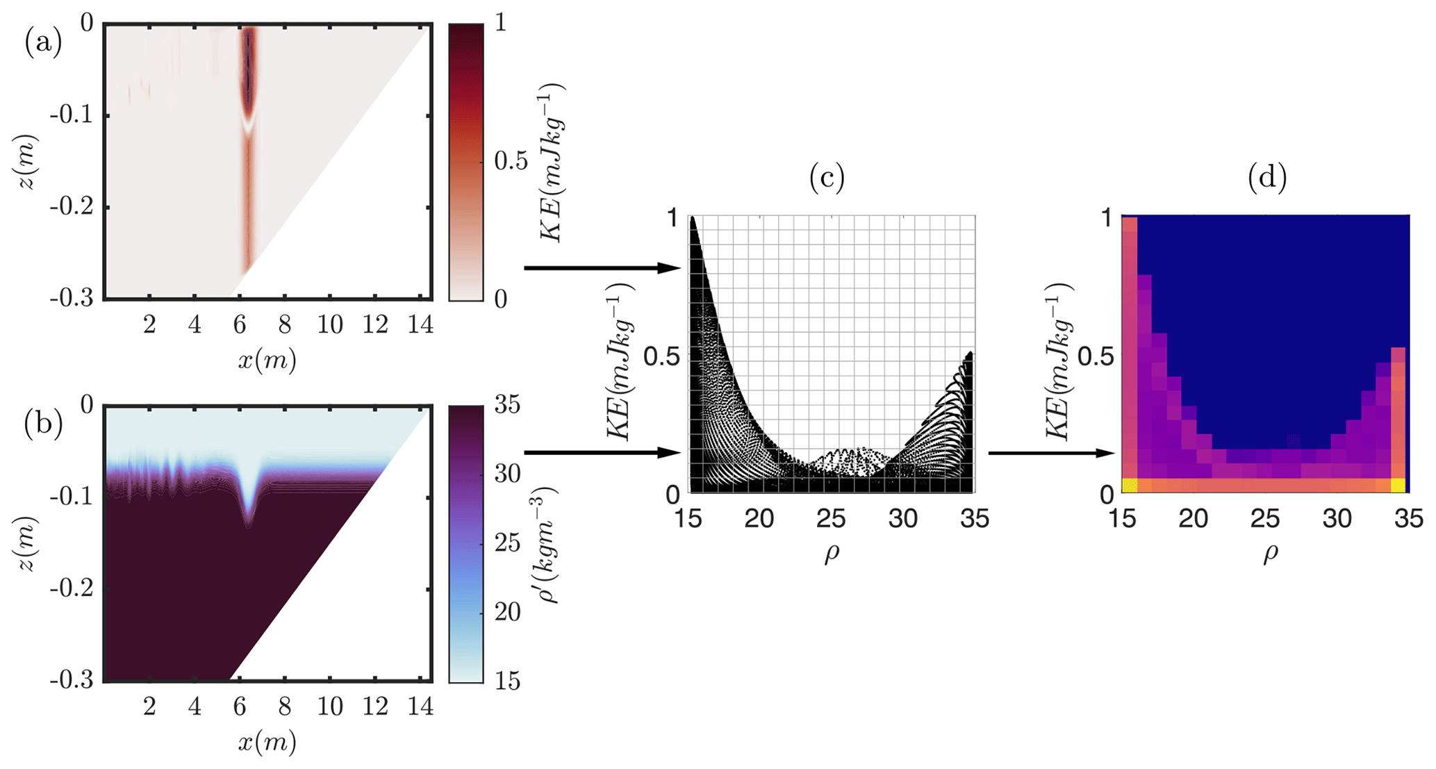
Figure 1Schematic of the creation of USP diagrams. The combination of two fluid properties (left) is represented in variable–variable space (centre) and then summed into discrete bins (right).
Following the method of Penney et al. (2020), the algorithm employed is applied as follows. For two variables ϕ and θ (which could for example represent density and kinetic energy), the domains are subdivided into Nϕ and Nθ bins, with sizes
For each grid cell, the nearest bin centre is identified:
For each grid cell, the Iij(ϕ,θ) is calculated:
and the total weight for each given bin with centre (ϕi,θj) is given by
Thus for a given bin, the weight Wij is the total volume of grid cells that had and . The end result of the process is a bivariate weighted histogram. The weighting ensures that the probability density function (PDF) reflects the probability a volume of fluid has given properties in mapped domain cases. A code for this applied to the numerical model SPINS (introduced in Sect. 2.2) can be found at https://github.com/HartharnSam/SPINS_USP (last access: 4 December 2023). This code generalises the formulation in Penney et al. (2020) to any two fluid variables and to a non-uniform grid (including mapped grids).
The second new tool introduced herein is the technique of region-of-interest (ROI) plots. Here, the variable is plotted in physical space but only where conditions identified on the paired histogram are met, for example, kg m−3 and Jkg−1. In relation to mixing in the shoaling wave simulations, the kinematic quantity investigated is enstrophy density, (where ), which describes the rotational energy linked to dissipation in 2-D flows and so is a quantity associated with (but not a measure of) mixing. The kinetic energy density, KE , is used as a measure of energy of translation in the flow.
In order to unambiguously identify time periods of interest in the various case studies reported on below, we have utilised the methodology of Shaw and Stastna (2019). Briefly, this technique computes the empirical orthogonal functions (EOFs) for a particular physical quantity using the built-in svds function in MATLAB. The EOFs are used to create reconstructions of the original physical field, and the infinity norm of the difference between the reconstruction and original field is plotted as a function of time and the number of modes used in the reconstruction. Time periods for which a jump in the number of EOFs is needed to obtain an approximation below a given error tolerance are taken as “periods of interest” and hence selected for detailed examination. This technique is attractive because it builds on a standard technique (EOFs) while addressing its well-known shortcoming (the fact that individual EOFs are not physical quantities).
2.2 Numerical model
Simulations were carried out with the pseudospectral code SPINS described in Subich et al. (2013). The code has been thoroughly validated using theoretical result and physical laboratory experiments in a number of different configurations, including shear instabilities, boundary layer instabilities (e.g. Harnanan et al., 2017), interaction with topography (e.g. Deepwell et al., 2017), and shoaling ISWs (e.g. Hartharn-Evans et al., 2022a). It is available for download through its online manual at https://wiki.math.uwaterloo.ca/fluidswiki/index.php?title=SPINS_User_Guide (last access: 4 December 2023).
The model solves the stratified Navier–Stokes equations subject to the Boussinesq approximation:
where u is the velocity, t is time, P is the pressure, Ξi is the passive tracer field, ρ is the density, and ρ0 is some reference density of the fluid; throughout this paper density is reported using the density perturbation . The physical parameters are gravity g (set at 9.81 m s−2), the shear viscosity ν (set at , chosen to be consistent with the physical value), and scalar diffusivity κρ (or for tracer). The unit vector in the vertical direction is denoted by . The boundary conditions, domain dimensions, and other varying parameters for each simulation are described for each case in Sect. 2.2.1 and 2.2.2.
2.2.1 Shoaling internal solitary waves
To illustrate the USP method, simulations from previously published papers on ISW shoaling will be utilised, namely simulations 27_111120 (here the surging case), 26_091120 (here the collapsing case), and 24_071020 (here the plunging case) from Hartharn-Evans et al. (2022a) and the Thin-20L case (here the fissioning case) from Hartharn-Evans et al. (2022b). Full details of the simulations can be found in the respective papers. ISWs were simulated in a rectangular tank with waves initiated using the lock gate technique and a slope at one end of the tank as shown in the schematic of the model set-up in Fig. 2a. The length of the tank Lx=7 m (extended to Lx=14.5 m for the fissioning case), and the depth of the tank Lz=0.3 m. A hyperbolic smoothing function produces the gate region by a numerical step in density 0.3 m from the left end of the tank, from which an ISW is produced and propagates from left to right.
No slip boundary conditions were applied at the flat upper and mapped lower boundaries to satisfy model requirements. A mapped Chebyshev grid is employed in the vertical, implying a clustering of points near both the upper and lower boundary that scales with the number of points in the vertical squared, and vertical resolution improves over the slope. Free-slip boundary conditions were applied at the vertically oriented left and right ends of the computational domain, the grid spacing of which was regularly spaced. Grid resolution was 4096 points in the x and 256 grid points in the z coordinate, giving dx=1.7 mm in all cases except the fissioning case, where dx=3.5 mm. Away from the slope, dz varies between 0.124 mm at the upper and lower boundaries and 1.8 mm near mid-depth, simulations were two-dimensional and m2 s−1.
The vertical density profile in the main tank was set according to the smoothed two-layer or hyperbolic tangent profile:
set for a system like that studied previously in the literature consisting of a thin, linearly stratified pycnocline (hpyc=0.015 m) sandwiched between homogeneous layers, here referred to as “thin tanh stratification”. The density change is Δρ=20 kg m−3, the reference density is ρ0=1026 kg m−3, and the depth of the pycnocline is zpyc=0.07 m. Simulations are carried out for a slope of s=0.2 in all cases except the fission case at s=0.033, and in all cases the slope height is 0.3 m, the full depth of the water column. The bottom boundary follows the form of Lamb and Nguyen (2009):
where
and d (=0.03) represents a characteristic distance for the transition from 0 to a constant slope of 1 and Ls the length of the slope (1.5 or 9 m for the fission case). The function smooths the transition from the flat bed to the slope, which is necessary for the spectral code. The surging (a=0.009 m), collapsing (a=0.048 m), and plunging (a=0.076 m) cases represent increasing wave amplitudes (a), and the fissioning (a=0.063 m) case has an intermediate wave amplitude.
2.2.2 Cold shear instability
A Kelvin–Helmholtz instability was produced for a three-dimensional (3-D) simulation in a domain 0.512 m in the x direction and 0.128 m in the y and z directions by initialising a temperature stratified shear flow perturbed with white noise. Free slip boundary conditions were applied at the upper and lower boundaries, with regular grid spacing in all dimensions and periodic boundary conditions in the x and y domains. To produce a stratified shear flow, the temperature field, T(z), and horizontal velocity field, u(z), were initialised as follows:
A nonlinear EOS suitable for cold, fresh water was chosen. The EOS to calculate densities from temperature and salinity is the polynomial fit from Brydon et al. (1999), assuming salinity and excess pressure are 0 everywhere. The background temperature and velocity gradient regions are thus in a similar location, but the density stratification is asymmetric (Fig. 2b). Salinity was set to 0 everywhere, and v and w were set at rest, with small white noise perturbations to initialise the instability. The interface depth, zmix, and thickness, hmix, were 0.064 and 0.01 m respectively. The minimum initial Richardson number, Ri0, is defined as
The configuration was set such that Ri0≪0.25 (=0.087). The low value was chosen because Ri=0.25 is the necessary, but not sufficient, criterion for shear instability. For this temperature range, the density range is very small, so for the cold shear instability cases, the density perturbation, ρ′, is a useful measure.
Figure 2(a) Shoaling ISW schematic diagram showing the numerical domain used for the shoaling internal solitary wave simulations in this study. (b) Cold shear instability schematic indicating the initial vertical profiles of the density, temperature, and velocity fields for the cold shear instability simulations (horizontal scales adjusted); the dashed horizontal line indicates the mid-tank and the centre of the interface for T and u.
Such flows characterise situations where the temperature and momentum are linked, rather than density and momentum, for example, a warm river flow entering a cold lake.
To establish the interplay between passive and active tracers, a passive tracer (i.e. dye in a laboratory setting) was additionally initialised in two further simulations with the same initial conditions as temperature (Eq. 12) but with each case performed at different tracer diffusivity to the temperature tracer, as described in Sect. 3.3.
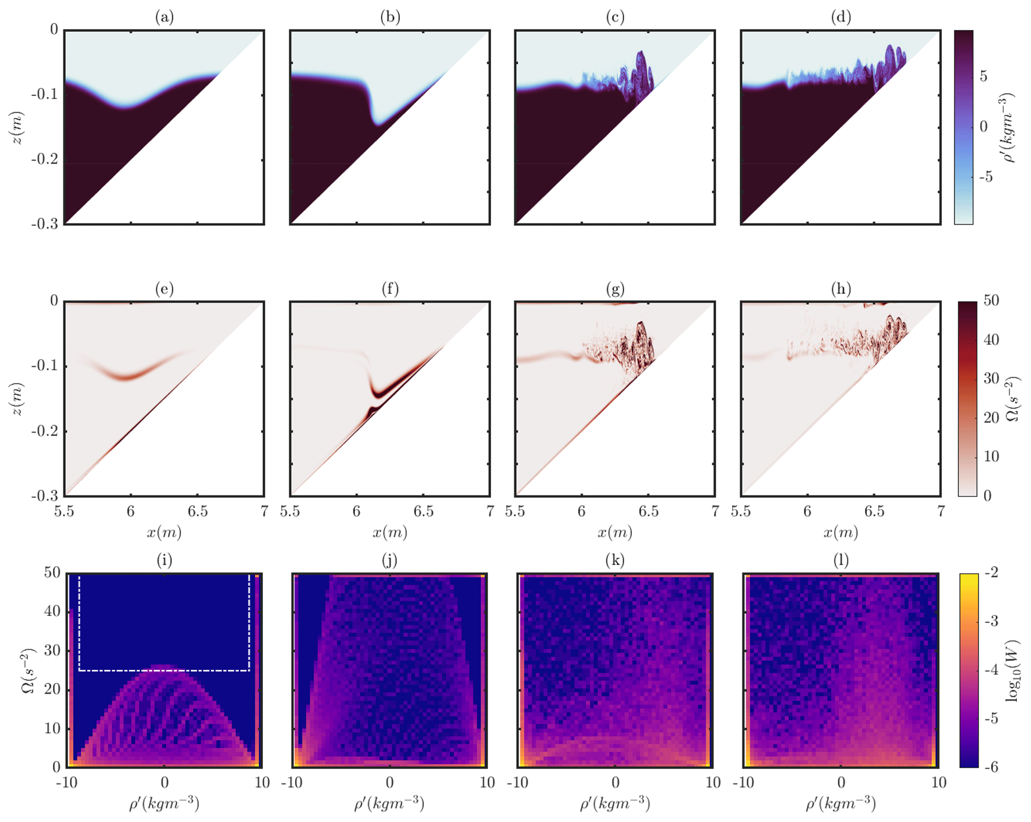
Figure 3Time sequence of collapsing wave shoaling process shown as ρ′ (top), Ω (middle), and the USP for the same variables (bottom). t= [55, 60, 70, 75] s.
3.1 Fissioning internal solitary waves and the newly mixed layer
The evolution of shoaling ISWs in this stratification takes one of four forms: surging, collapsing, plunging, or fissioning (for more details, see, for example, Sutherland et al., 2013; Hartharn-Evans et al., 2022a). Each of these manifests different mixing and dissipation characteristics, as identified via bulk mixing measures (Arthur and Fringer, 2014). Figure 3 shows the evolution of one of these examples collapsing, which occurs with moderate steepness waves over moderate slopes; this will be explored here in more detail (each of the other examples is presented in Figs. S1–S3 in the Supplement). A more complete description of these processes can be found in Hartharn-Evans et al. (2022a) Sect. 4.3, but here the focus is on the evolution of USPs during this process.
First, the reference USP case for an ISW prior to interacting with the slope, as shown in Fig. 1, is explored. At this point, most of the fluid in a three-layer stratification is at either extreme of density (ρ=1015 or 1035 kg m−3) (Fig. 1b, d), with only a small amount of fluid in intermediate densities across a thin pycnocline. Meanwhile, the KE is strong in both the upper and lower layers around the wave itself (Fig. 1a) and is small at the centre of the pycnocline due to shear here. The overall result is an arcing pattern in USP space. This pattern is asymmetric, due to the asymmetric stratification (in the vertical), which concentrates the KE in the upper layer. In order to investigate mixing due to the shoaling of this wave, we will now explore how this pattern changes during the shoaling process and identify the fluid regions which these new fluid properties apply to, instead using enstrophy, where Ω is a measure of energy in the flow available for mixing. Almost inverse to the KE USP in Fig. 1, Ω is highest at the highest shear region across the pycnocline in the wave and at the upper and lower boundaries around the wave (Fig. 3i).
As the wave begins to interact with the slope and steepen (Fig. 3a, b, e, f), a separation bubble forms on the slope due to boundary layer separation (Carr et al., 2008; Boegman and Ivey, 2009); meanwhile enstrophy remains constrained to the pycnocline (now extended), and the separation bubble is reflected in much higher enstrophy across mid-densities (Fig. 3f, j). As the wave continues to propagate upslope and concentrate into a shallower region, the separation bubble strengthens and produces what is sometimes termed a “global” instability (Fig. 3c, g). The USP reveals higher enstrophy primarily associated with higher densities, with remnants of the high enstrophy at the upper and lower boundaries still visible in the USP as the high enstrophy at high and low density limits (Fig. 3g, k). This evolves into a bolus of fluid moving upslope (Fig. 3d, h). Although plots of enstrophy and density indicate mixing is occurring around the pycnocline at the head of the bolus (Fig. 3d, h), the USP is informative of where mixing is occurring. As the bolus propagates upslope, the skew of high enstrophy fluid towards higher densities (lower-layer fluid) becomes clearer in the USP diagram (Fig. 3l).
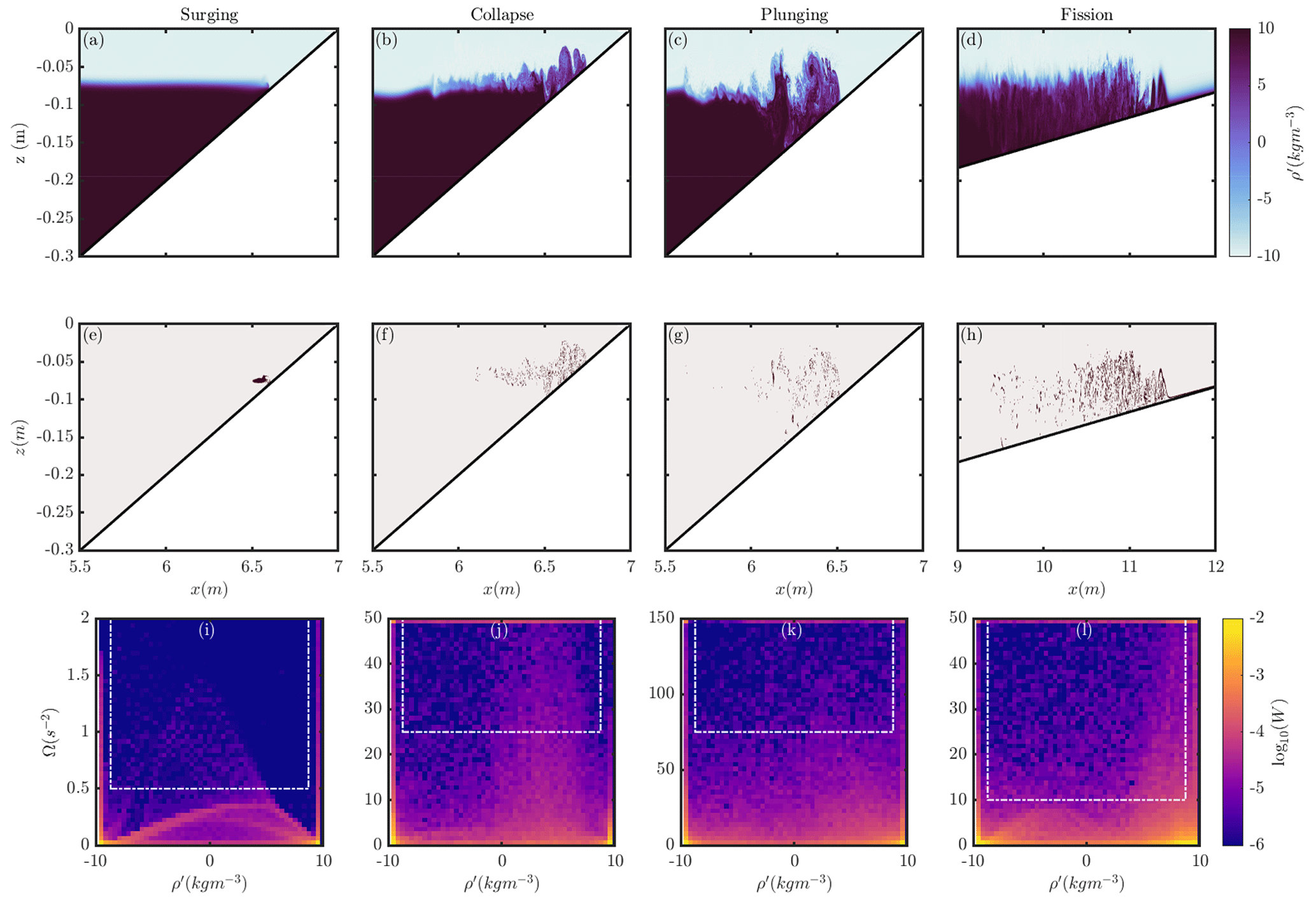
Figure 4Four example waves representing different breaking regimes at a late time step, showing density (top); region of interest (ROI; middle), where the fluid meeting the criteria is marked in dark red; and the USP (bottom). The white box in the lower panels indicates the ROI selected, based on the USP at earlier time steps.
A region of USP space can be identified at early output times, which includes only Ω higher than that associated with a stable ISW, and intermediate densities, and therefore is taken here to represent active mixing regions (white box Fig. 3i). The fluid that has the properties contained within such a region can be identified and is plotted in Fig. 4e–h, for each type of wave shoaling. For a collapsing wave at a late time step, this shows a large continuous patch of actively mixing fluid, extending over around 0.7 m (Fig. 4f), concentrated at intermediate densities (the pycnocline), although slightly skewed towards higher densities (Fig. 4j).
Following this same process for four example waves across the four breaking regimes reveals their mixing properties. Surging is observed for small amplitude waves, and the resulting process is a non-turbulent surge of dense fluid propagating upslope (Fig. 4a). A single region of high enstrophy forms as the combination of that at the pycnocline and the lower boundary (Fig. 4e), and this is advected upslope. Little mixing occurs during this process (Fig. 4i), and the small active mixing region is advected upslope in the pulse of dense fluid. Plunging, which takes place at high slope and wave steepness values, results in an anvil-shaped instability plunging forward from the rear steepening face of the wave. As a result, overturning occurs, and this process has been associated with high levels of mixing. Although this process produces high enstrophy across the density range, indicating a lot of mixing (Fig. 4k), the actively mixing fluid is less continuous and stretches over a smaller horizontal extent than a collapsing wave (Fig. 4c, g). The active mixing region is vertically extensive, reflected in the USP with high enstrophy across all densities, but a slight skew in the USP diagram indicates mixing is associated with lower densities mixing with intermediate densities rather than higher densities with intermediate densities. The final wave shoaling behaviour, fissioning, is shown in the right column of Fig. 4 and occurs over gentle slopes. The formation of multiple dense pulses of fluid (Fig. 4d), which in this example are quasi-turbulent, produces actively mixing fluid over a long horizontal extent (Fig. 4h), with active mixing occurring as the pulses propagate upslope. A strong skew in the USP indicates mixing is primarily associated with high densities and therefore the lower layer (Fig. 4l). This follows with the concept of dense pulses propagating upslope and mixing as they do so.
As an overview of this pattern, as the wave steepness increases, and therefore the wave breaking regime moves from surging through collapsing to plunging, the region of actively mixing fluid increases. Fissioning takes this a step further; with a similar input wave to the collapsing case, the gentle slope allows the wave to mix over a longer distance.
3.2 Cold shear instability
The unstable shear flow undergoes the typical evolution through the formation of Kelvin–Helmholtz (K-H) instability, as follows. Initially, the flow is a shear flow in stably stratified fluid (Fig. 5a, e), where the kinetic energy (KE) is high in both the upper and lower layers but at the interface of the layers is zero, at the inflection point of the horizontal velocity (Fig. 2b). As the fluid is a two-layered shear flow, one would expect the KE USP to be a symmetrical curve, where the highest kinetic energy is associated with the highest- and lowest-density anomalies away from the interface (which is also where most of the fluid resides), whilst intermediate densities represent the shear layer where KE is lower. Here, the KE USP shows a “crooked smiley face”, with most of the fluid concentrated at the extremes of density, but due to the temperature stratification and nonlinear EOS, the curve is shifted towards higher densities (Fig. 5i). Despite kinetic energy being high at this stage in the other directions, there is very little kinetic energy in the y direction (KE), indicating the flow features at this stage are not dependent upon 3-D elements of the flow (Fig. 5i, m).
It is worth noting that while the evolution of the shear instability is generic, the nonlinearity of the EOS means that the symmetry across the centre of the co-located shear and density layers is broken. The visual manifestation of the billows is effectively slightly biased toward one side.
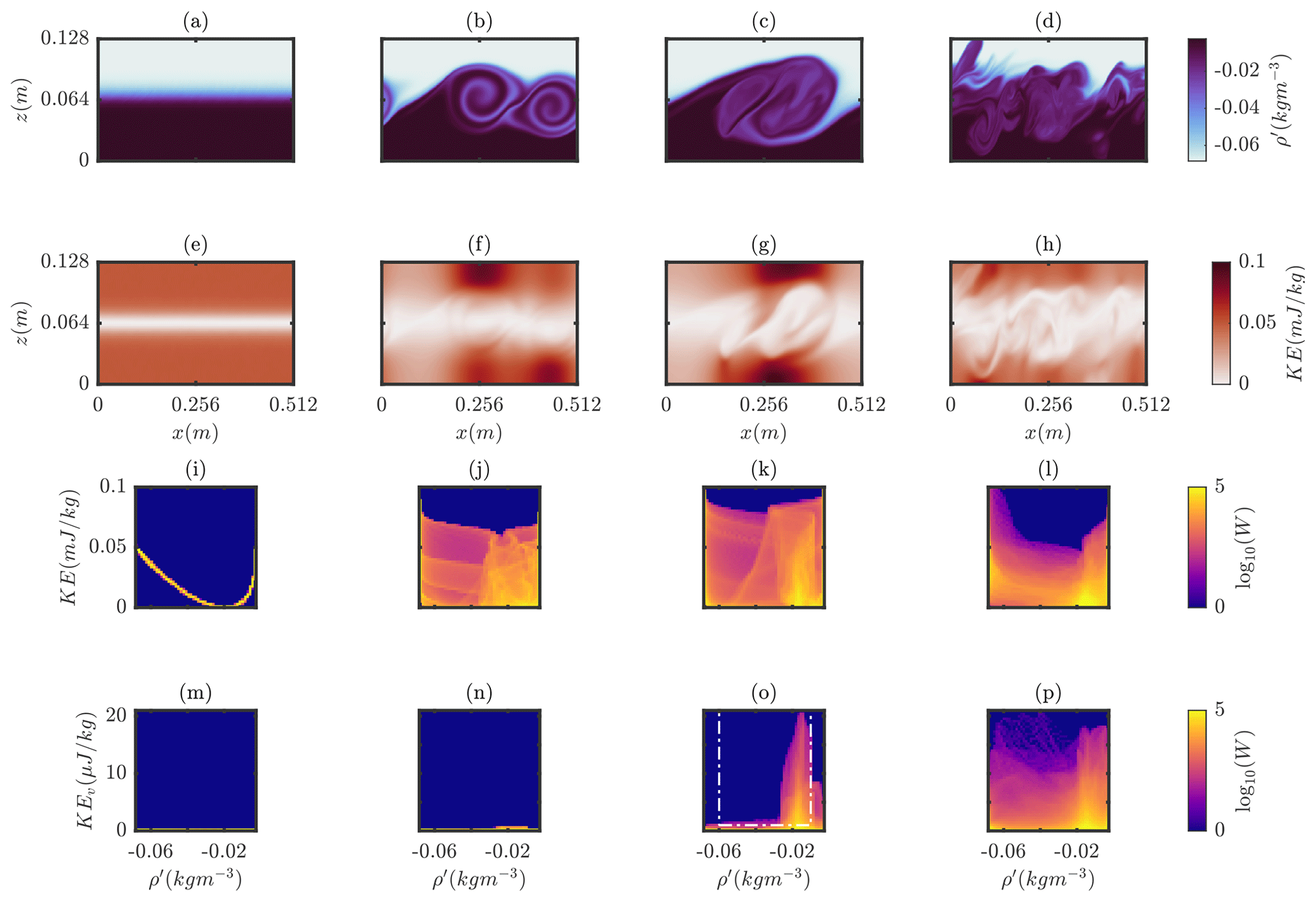
Figure 5Time sequence of the cold shear instability, shown as density (a–d) and kinetic energy density (e–h) fields, and the USP for density vs KE density (i–l) and for density vs KEv (the KE density for just the v component) (m–p). t=[5, 170, 225, 275] s.
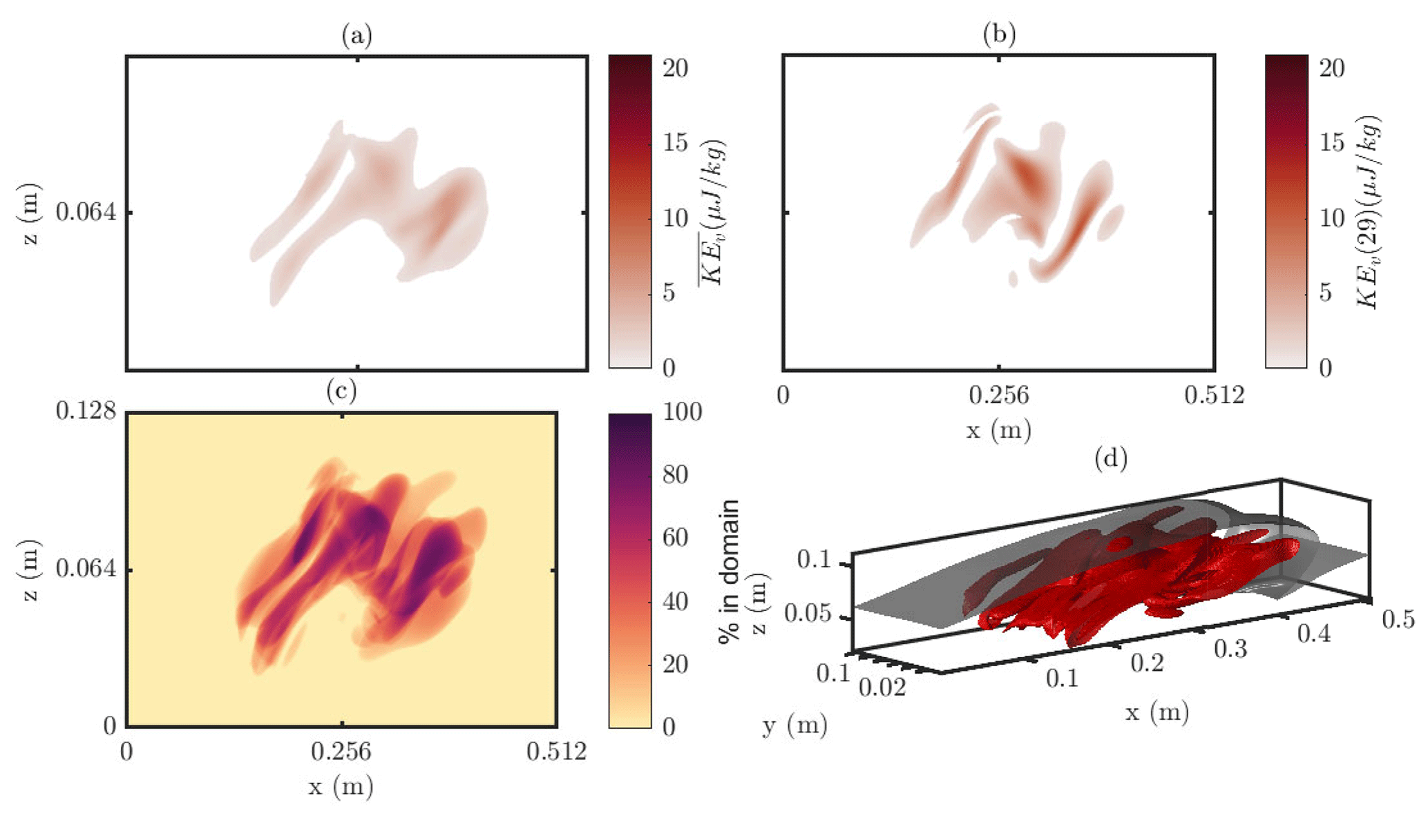
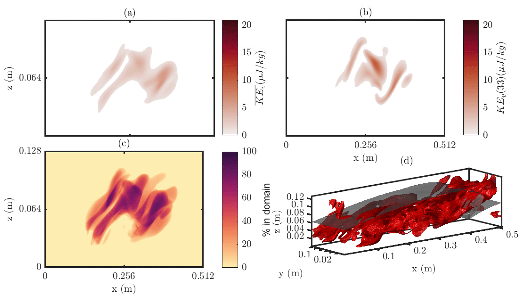
Figure 6Regions of interest of the cold shear instability case at t=225s, based on the region indicated in the white box of Fig. 5o. Shown as the ROI in the transverse mean KEv field (a), the KEv x,z slice most representative of the mean (b), the proportion of the y domain within the ROI for the (x,z) plane (c), and the boundaries of the ROI (red) with the kg m−3 isopycnal for reference (black) (d).
Small fluctuations in the flow result in stationary waves growing on the interface, which, due to the shear, grow and roll up, forming braids and billows (Fig. 5b, f). As the billows form and stretch, an increasing amount of the flow's KE builds around the billows and is therefore associated with the intermediate densities (Fig. 5f, j). Until now, the flow is two-dimensional, with negligible kinetic energy in the transverse direction (Fig. 5m, n) and little transverse variability. During the braiding and billow growth, the pycnocline is stretched thin (Fig. 5b), enhancing the potential for mixing by stretching density gradients. The roll up of these billows is such that alternating layers of high and low density form, with the density now statically unstable, leading to turbulence (and in turn spanwise instability) and mixing. These billows pair and coalesce by t=225 s (Fig. 5c). The kinetic energy associated with intermediate densities continues to build as the billows coalesce, but by this stage, an increased volume of fluid that represents fluid in the to −0.01 kg m−3 range is evident (Fig. 5k), indicating that mixing has occurred in the fluid. When the billows coalesce, KEv is high, and almost all of this is associated with the same density range as that of the newly mixed fluid layer at late stages (Fig. 5o). This indicates the importance of these transverse flow features in the mixing produced by billows formed from a K-H instability. The skew in the density of newly mixed fluid, as a result of the cold temperature nonlinearity in density, is to some extent visible (but easily missed) in the ρ′ plots (Fig. 5c) but is only truly apparent in USP space (Fig. 5k, l, o, p).
Beyond this time, mixing across the braids continues and leads to a new state (Fig. 5d) where a quasi-turbulent intermediate density layer forms, which represents a new steady state, where the Ri is reduced by a smoothed density gradient. As the flow begins to settle back towards the new steady state, kinetic energy at the intermediate densities falls, with the presence of the layer of intermediate density evident at kg m−3.
The USP region in which active mixing is related to 3-D processes is identified in Fig. 5o. This is where KEv is higher than any of the flow in early time steps and with intermediate density. This region of the flow for t=225 s is isolated in Fig. 6. The transverse average KEv (Fig. 6a) shows that this active 3-D mixing is occurring right at the core of the K-H billow, whilst there is considerable variability throughout the y direction (Fig. 6c, d). Peaks in KEv are particularly localised (Fig. 6b), indicating the small-scale processes at play responsible for the mixing. Such results are indicative of the importance of 3-D simulations for understanding these mixing processes. By isolating the fluid undergoing these processes, we can identify regions of the flow worthy of future study.
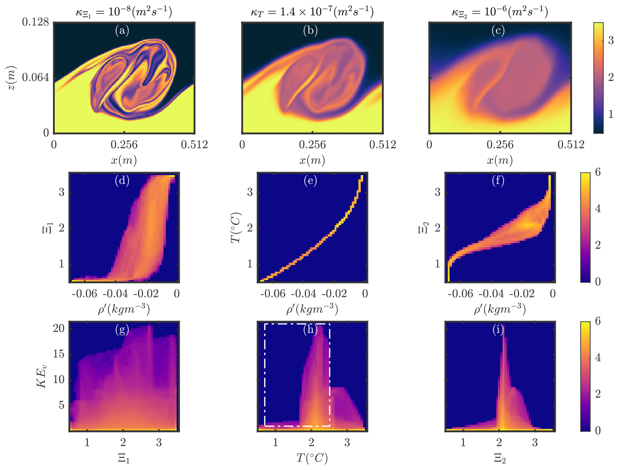
Figure 7Late time step (t=225 s) plots for the K-H Dye 1 case (a, d, g), the base case (b, e, h), and the K-H Dye 2 case (c, f, i). Panels (a), (b), and (c) show the tracer field (tracer for the K-H Dye case 1 and 2, temperature for base case); panels (d), (e), and (f) show the density vs tracer USP; and panels (g), (h), and (i) show tracer vs KEv.
3.3 Cold shear instability with passive tracers
Two additional simulations were carried out with a passive tracer, Ξi, with different prescribed diffusivities. A less diffusive case (case K-H Dye 1) had m2 s−1 (case K-H Dye 1), and a more diffusive case (case K-H Dye 2) had m2 s−1. These represent diffusivity approximately 1 order of magnitude lower and greater than the active temperature field, m2 s−1. A snapshot taken of the time step at which billows coalesce (t=225 s) reveals the emergence of fine structures in the K-H Dye 1 case within the billow core, with sharp interfaces (Fig. 7a), and a much more diffuse core, with blurred interfaces in the K-H Dye 2 case (Fig. 7c). Such features manifest in the USP of the tracer against density (Fig. 7 middle row). A control with the active temperature tracer is presented (Fig. 7e), indicating the nonlinear relationship between density and temperature. The skew of this Fig. to the K-H Dye 1 case (Fig. 8d) shows which gradient is diffused faster, here indicating that the density gradient is diffusing faster than the tracer, that is that the extremes of salinity, associated with the upper- and lower-layer fluids initially, now map onto a range of densities. Meanwhile, the skew of this Fig. to the K-H Dye 2 case (Fig. 7f) shows that the tracer gradient is diffusing faster than the density, that is that the extremes of density, associated with the upper- and lower-layer fluids, now map onto a range of densities and indicate that if the fluids were sorted again by density, each layer would contain varying levels of the tracer (that is to say, the tracer has been mixed).
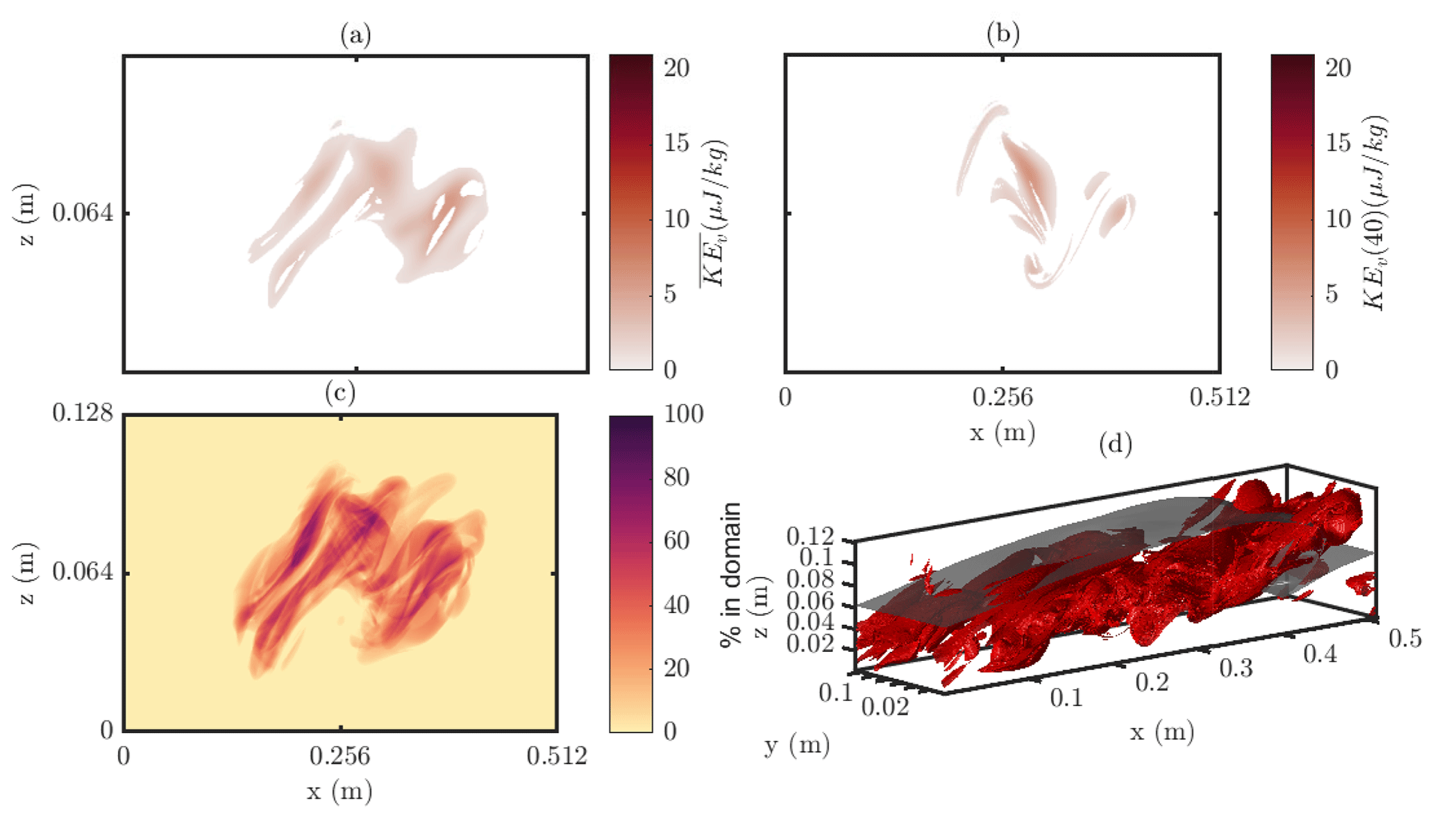
Applying the same region of active 3-D mixing (based on the density of that fluid at the initiation of the simulation), as in Fig. 6 (see region in Fig. 7h), produces Figs. 8 and 9. The mixing of the less diffusive passive dye indicates a pattern of highly localised, filamentous structures that are regions of active dye mixing (Fig. 8b–d). In contrast, the diffusive passive dye is mixing in broader-scale structures (Fig. 9c). However, the large-scale regions in which this passive dye is mixing is similar across both simulations (Figs. 8a, c 9a, c), indicating that there is an important interplay between the large-scale flow structures (the K-H billow and overturn of the isopycnals shown as the black isosurface) and filamentous fine-scale structures, across which the diffusive dye is able to diffuse. This result highlights the small scales at which diffusion plays an important role; only once the fluid and associated gradients are stretched to fine scales does the difference in diffusivity between dyes (and indeed the active tracer in Fig. 6) play any role.
By pairing a kinematic measure (KE, KEv, or Ω) with a conserved tracer (density, temperature, or passive dye), the role of both turbulence in stirring the fluid and diffusive processes in irreversibly blurring density gradients is shown for several example stratified flows. This process has also been used to identify which fluid constituents are being mixed more effectively by a given process, whether the low-density, upper-layer fluid is being mixed into the pycnocline, or higher-density, lower-layer fluid is being mixed upwards, and the eventual fate of these fluids. In the case of the shoaling ISWs, it is used to evidence whether mixed fluids are retained locally to the site of mixing, advected upslope, or advected away from the slope as an intermediate (or nepheloid) layer. Each of these questions is difficult to answer using existing bulk energetics models. The USP method has an additional advantage over existing methods for understanding in its ease of implementation and its reliability, in cases where the model is under-resolved or has non-trivial bathymetry.
The results from shoaling ISWs reveal considerably different mixing regimes between breaking types, for example, the horizontal extents of mixing between collapsing and plunging, where past studies have identified similar results between breaking types based on the energetics-based mixing measures alone. However, whilst it may be the bulk measure that is most useful in parameterising global-scale models, the locality of mixing, and transport of this fluid, which may carry with it nutrients, heat (i.e. thermal refuge for biota), and sediment (depending on the local geomorphological setting), is crucial to understand the effects of such processes on ecosystems. The features outlined by ROI in some shoaling ISW examples (e.g. Fig. 3h) have a striking similarity to the intermediate nepheloid layers identified by Bourgault et al. (2014), formed due to the shoaling of ISWs and the interaction of sediment resuspension and mixing. Similar features have been observed in various locations, but due to their episodic nature, their formation mechanisms can be unclear (Schulz et al., 2021). Understanding how these features form and evolve may help understand how such features may contribute to larger-scale sediment fluxes and, as a result, carbon exports (Schulz et al., 2021). To investigate these processes, the USP method could be applied with an active sediment tracer.
For the cold shear instability, these results also reveal new insights into the dynamics of shear flows at low temperatures (below the density maximum). The shear flow presented could represent a cold river flow into a lake, and as such the position of the velocity gradient and temperature gradient are linked, whilst the density gradient position is offset. The result of this in the shear flow is to produce asymmetric K-H features (e.g. Fig. 5b) and mixing bias towards one density (Fig. 5o). These asymmetric stratified shear flows have attracted recent attention following field observations (e.g Tu et al., 2020; Olsthoorn et al., 2023). Previous work on K-H billows has highlighted the role of 3-D instabilities beyond the point at which billows coalesce. Here, isolating the fluid where these 3-D (v) flows are playing an active part in mixing shows not only that are 3-D processes important at this stage but also that they remain within the coalesced billow region and at a small scale (Fig. 6). Beyond that stage, this v component of the KE remains high around the active mixing region but also increasingly across the entire flow. Furthermore, investigating the mixing of passive tracers is also not possible using energetics models and has been presented here, identifying which densities the mixing of passive tracers is associated with and the role of 3-D instabilities in the passive tracer mixing processes.
The USP method identifies how the different regimes of mixing associated with different breaking types (and therefore with differing wave and slope characteristics) manifest themselves. ISWs breaking with surging behaviour produce a small mixing region, which is advected upslope, indicating transport of the mixed fluids, potentially to regions of high biological activity. In contrast, collapsing ISWs produce a large patch of actively mixing fluid over a long horizontal area, particularly with lower-layer fluid mixed up into the pycnocline. Plunging ISWs, which initially appear to have similarities to collapsing ISWs, are instead dominated by upper layers mixed down into the pycnocline and are more horizontally constrained. Finally, ISWs undergoing fissioning produce active mixing over a long horizontal region, advected upslope in the form of quasi-turbulent dense pulses (i.e. boluses). Temperature-stratified shear flow simulations in the cold, nonlinear EOS regime reveal important differences with a density-stratified shear flow. The USP at early time steps immediately reveals the asymmetry of the distribution of density and kinetic energy, an asymmetry which goes on to play an important role in the mixing induced by the shear instability. Once density gradients have been stretched, and transverse flow at medium–high densities forms, mixing occurs in an asymmetric manner, producing a late-stage state with the layer of newly mixed fluid skewed towards medium–high densities. Simulations of the shear flow with passive tracers of varying diffusivity highlight the nature of flow structures associated with mixing fluid. At low diffusivities, filamentous structures in the tracer are observed, heavily associated with 3-D elements of the flow, whilst at high diffusivity, tracer gradients are blurred. Both scenarios show interplay between the dynamic drivers in large-scale flow features and diffusive effects at filamentous fine scales once large gradients are produced by stretching. Such fine-scale structures are revealed by the new ROI plots based on the USP double histograms. Overall, the new USP method provides valuable insights into the evolution and dynamics of sheared flows and the role of temperature-based stratification within the nonlinear EOS regime and diffusivity in mixing processes in particular.
The USP method provides a method of interpreting and investigating mixing that is not blind; i.e. it invites the researcher to understand the ongoing processes in a way that is ignored by the relative black box of typical (bulk) mixing methods. The tagging of particles based on variables provides a methodology that lies somewhere between a strictly Eulerian and strictly Lagrangian approach to understanding mixing. In the case of the passive tracer, the method has been used to trace the motion of specific parcels of fluid. This could be further refined by introducing the tracer at different times in the simulation into localised regions of interest. Future work could also set up higher dimensional histograms (although these become increasingly difficult to visualise) and/or more complex selection criteria based on multiple quantities, effectively a language to classify aspects of the fluid motion.
The interactive MATLAB tool presented in this study can be found at https://github.com/HartharnSam/SPINS_USP (last access: 4 December 2023). This code and data are available from https://doi.org/10.25405/data.ncl.c.6704289 (Hartharn-Evans et al., 2023).
The supplement related to this article is available online at: https://doi.org/10.5194/npg-31-61-2024-supplement.
SGHE and MS performed, analysed, and curated data from the numerical simulations; produced the analysis code; and were responsible for study conceptualisation and design and writing of the original draft. SGHE was responsible for visualisation, MC and MS were responsible for resource acquisition and supervision, and all authors reviewed and edited the manuscript and contributed to funding acquisition.
The authors have declared that none of the authors have any competing interests.
Publisher's note: Copernicus Publications remains neutral with regard to jurisdictional claims made in the text, published maps, institutional affiliations, or any other geographical representation in this paper. While Copernicus Publications makes every effort to include appropriate place names, the final responsibility lies with the authors.
This article is part of the special issue “Turbulence, wave–current interactions, and other nonlinear physical processes in lakes and oceans”. It is a result of the EGU General Assembly 2023 session NP6.1 Turbulence, wave-currents interactions and other nonlinear physical processes in lakes and oceans, Vienna, Austria, 25 April 2023.
This work was supported by the Natural Environment Research Council (NERC)-funded ONE Planet Doctoral Training Partnership (Samuel George Hartharn-Evans, grant no. NE/S007512/1) and a Turing Global Fellowship (Samuel George Hartharn-Evans). This work made use of the Rocket High Performance Computing service at Newcastle University and the Math Faculty Computing Facility at the University of Waterloo. Partial funding for travel was provided by the Natural Science and Engineering Research Council of Canada RGPIN-311844-37157. Exploratory computations and discussions of these with Karem Abdul-Samad and Chris Subich are gratefully acknowledged. Two anonymous reviewers are thanked for contributions to this paper.
This research has been supported by the Natural Environment Research Council (grant no. NE/S007512/1) and the Natural Sciences and Engineering Research Council of Canada (grant no. RGPIN-311844-37157).
This paper was edited by Kateryna Terletska and reviewed by two anonymous referees.
Aghsaee, P., Boegman, L., and Lamb, K. G.: Breaking of Shoaling Internal Solitary Waves, J. Fluid Mech., 659, 289–317, https://doi.org/10.1017/S002211201000248X, 2010. a
Arthur, R. S. and Fringer, O. B.: The Dynamics of Breaking Internal Solitary Waves on Slopes, J. Fluid Mech., 761, 360–398, https://doi.org/10.1017/jfm.2014.641, 2014. a
Arthur, R. S., Koseff, J. R., and Fringer, O. B.: Local versus Volume-Integrated Turbulence and Mixing in Breaking Internal Waves on Slopes, J. Fluid Mech., 815, 169–198, https://doi.org/10.1017/jfm.2017.36, 2017. a
Boegman, L. and Ivey, G. N.: Flow Separation and Resuspension beneath Shoaling Nonlinear Internal Waves, J. Geophys. Res.-Oceans, 114, 2018, https://doi.org/10.1029/2007JC004411, 2009. a
Bourgault, D., Morsilli, M., Richards, C., Neumeier, U., and Kelley, D. E.: Sediment Resuspension and Nepheloid Layers Induced by Long Internal Solitary Waves Shoaling Orthogonally on Uniform Slopes, Cont. Shelf Res., 72, 21–33, https://doi.org/10.1016/j.csr.2013.10.019, 2014. a
Brydon, D., Sun, S., and Bleck, R.: A New Approximation of the Equation of State for Seawater, Suitable for Numerical Ocean Models, J. Geophys. Res.-Oceans, 104, 1537–1540, https://doi.org/10.1029/1998JC900059, 1999. a
Caldwell, D. R.: Oceanic Turbulence: Big Bangs or Continuous Creation?, J. Geophys. Res.-Oceans, 88, 7543–7550, https://doi.org/10.1029/JC088iC12p07543, 1983. a
Carr, M., Davies, P. A., and Shivaram, P.: Experimental Evidence of Internal Solitary Wave-Induced Global Instability in Shallow Water Benthic Boundary Layers, Phys. Fluid., 20, 066603, https://doi.org/10.1063/1.2931693, 2008. a
Carr, M., Franklin, J., King, S. E., Davies, P. A., Grue, J., and Dritschel, D. G.: The Characteristics of Billows Generated by Internal Solitary Waves, J. Fluid Mech., 812, 541–577, https://doi.org/10.1017/jfm.2016.823, 2017. a, b
Caulfield, C.: Layering, Instabilities, and Mixing in Turbulent Stratified Flows, Annu. Rev. Fluid Mech., 53, 113–145, https://doi.org/10.1146/annurev-fluid-042320-100458, 2021. a
Caulfield, C. P. and Peltier, W. R.: The Anatomy of the Mixing Transition in Homogeneous and Stratified Free Shear Layers, J. Fluid Mech., 413, 1–47, https://doi.org/10.1017/S0022112000008284, 2000. a
Deepwell, D., Stastna, M., Carr, M., and Davies, P. A.: Interaction of a Mode-2 Internal Solitary Wave with Narrow Isolated Topography, Phys. Fluid., 29, 076601, https://doi.org/10.1063/1.4994590, 2017. a
Geyer, W. R., Lavery, A. C., Scully, M. E., and Trowbridge, J. H.: Mixing by Shear Instability at High Reynolds Number, Geophys. Res. Lett., 37, L22607, https://doi.org/10.1029/2010GL045272, 2010. a
Gibson, C. H.: Fossil Turbulence Revisited, J. Mar. Syst., 21, 147–167, https://doi.org/10.1016/S0924-7963(99)00024-X, 1999. a
Grace, A. P., Stastna, M., Lamb, K. G., and Andrea Scott, K.: Asymmetries in Gravity Currents Attributed to the Nonlinear Equation of State, J. Fluid Mech., 915, A18, https://doi.org/10.1017/jfm.2021.87, 2021. a, b, c
Harnanan, S., Stastna, M., and Soontiens, N.: The Effects of Near-Bottom Stratification on Internal Wave Induced Instabilities in the Boundary Layer, Phys. Fluid., 29, 016602, https://doi.org/10.1063/1.4973502, 2017. a
Hartharn-Evans, S. G., Carr, M., Stastna, M., and Davies, P. A.: Stratification Effects on Shoaling Internal Solitary Waves, J. Fluid Mech., 933, https://doi.org/10.1017/jfm.2021.1049, 2022a. a, b, c, d, e
Hartharn-Evans, S. G., Stastna, M., and Carr, M.: Dense Pulses Formed from Fissioning Internal Waves, Environ. Fluid Mech., 23, 389–405, https://doi.org/10.1007/s10652-022-09894-x, 2022b. a
Hartharn-Evans, S., Carr, M., and Stastna, M.: A new approach to understanding fluid mixing in process-study models, Newcastle University Collection [data set], https://doi.org/10.25405/data.ncl.c.6704289.v1, 2023. a
Helland-Hansen, B.: Nogen Hydrografiske Metoder, Forh Skand Naturf Mote, 16, 357–359, 1916. a
Imasato, N., Nagashima, H., Takeoka, H., and Fujio, S.: Diagnostic Approaches on Deep Ocean Circulation, in: Deep Ocean Circulation, edited by: Teramoto, T., vol. 59, Elsevier Oceanography Series, 307–331, Elsevier, https://doi.org/10.1016/S0422-9894(08)71334-5, 1993. a
Lamb, K. G.: On the Calculation of the Available Potential Energy of an Isolated Perturbation in a Density-Stratified Fluid, J. Fluid Mech., 597, 415–427, https://doi.org/10.1017/S0022112007009743, 2008. a, b
Lamb, K. G. and Nguyen, V. T.: Calculating Energy Flux in Internal Solitary Waves with an Application to Reflectance, J. Phys. Oceanogr., 39, 559–580, https://doi.org/10.1175/2008JPO3882.1, 2009. a
Lincoln, B. J., Rippeth, T. P., and Simpson, J. H.: Surface Mixed Layer Deepening through Wind Shear Alignment in a Seasonally Stratified Shallow Sea, J. Geophys. Res.-Oceans, 121, 6021–6034, https://doi.org/10.1002/2015JC011382, 2016. a
Michallet, H. and Ivey, G. N.: Experiments on Mixing Due to Internal Solitary Waves Breaking on Uniform Slopes, J. Geophys. Res.-Oceans, 104, 13467–13477, https://doi.org/10.1029/1999jc900037, 1999. a
Moum, J. N., Farmer, D. M., Smyth, W. D., Armi, L., and Vagle, S.: Structure and Generation of Turbulence at Interfaces Strained by Internal Solitary Waves Propagating Shoreward over the Continental Shelf, J. Phys. Oceanogr., 33, 2093–2112, https://doi.org/10.1175/1520-0485(2003)033<2093:SAGOTA>2.0.CO;2, 2003. a, b
Olsthoorn, J., Kaminski, A. K., and Robb, D. M.: Dynamics of Asymmetric Stratified Shear Instabilities, Phys. Rev. Fluids, 8, 024501, https://doi.org/10.1103/PhysRevFluids.8.024501, 2023. a
Peltier, W. R. and Caulfield, C. P.: Mixing Efficiency in Stratified Shear Flows, Annu. Rev. Fluid Mech., 35, 135–167, https://doi.org/10.1146/annurev.fluid.35.101101.161144, 2003. a
Penney, J., Morel, Y., Haynes, P., Auclair, F., and Nguyen, C.: Diapycnal Mixing of Passive Tracers by Kelvin-Helmholtz Instabilities, J. Fluid Mech., 900, 26–26, https://doi.org/10.1017/jfm.2020.483, 2020. a, b, c, d, e, f, g
Pope, S. B.: Turbulent-Viscosity Models, in: Turbulent Flows, Cambridge University Press, Cambridge, ISBN 9780511840531, https://doi.org/10.1017/CBO9780511840531, 2000. a
Salmon, R.: Lectures on Geophysical Fluid Dynamics, Oxford University Press, Oxford, New York, ISBN 978-0-19-510808-8, 1998. a
Schulz, K., Büttner, S., Rogge, A., Janout, M., Hölemann, J., and Rippeth, T. P.: Turbulent Mixing and the Formation of an Intermediate Nepheloid Layer Above the Siberian Continental Shelf Break, Geophys. Res. Lett., 48, e2021GL092988, https://doi.org/10.1029/2021GL092988, 2021. a, b
Scotti, A. and White, B.: Diagnosing Mixing in Stratified Turbulent Flows with a Locally Defined Available Potential Energy, J. Fluid Mech., 740, 114–135, https://doi.org/10.1017/jfm.2013.643, 2014. a
Shaw, J. and Stastna, M.: Feature Identification in Time-Indexed Model Output, PLOS ONE, 14, e0225439, https://doi.org/10.1371/journal.pone.0225439, 2019. a
Subich, C. J., Lamb, K. G., and Stastna, M.: Simulation of the Navier-Stokes Equations in Three Dimensions with a Spectral Collocation Method, Int. J. Numer. Meth. Fl., 73, 103–129, https://doi.org/10.1002/fld.3788, 2013. a
Sutherland, B. R., Barrett, K. J., and Ivey, G. N.: Shoaling Internal Solitary Waves, J. Geophys. Res.-Oceans, 118, 4111–4124, https://doi.org/10.1002/jgrc.20291, 2013. a, b
Thorpe, S. A.: Turbulence and Mixing in a Scottish Loch, Philos. T. Roy. Soc. Lond. A, 286, 125–181, https://doi.org/10.1098/rsta.1977.0112, 1977. a
Tu, J., Fan, D., Lian, Q., Liu, Z., Liu, W., Kaminski, A., and Smyth, W.: Acoustic Observations of Kelvin-Helmholtz Billows on an Estuarine Lutocline, J. Geophys. Res.-Oceans, 125, e2019JC015383, https://doi.org/10.1029/2019JC015383, 2020. a
Winters, K. B., Lombard, P. N., Riley, J. J., and D'Asaro, E. A.: Available Potential Energy and Mixing in Density-Stratified Fluids, J. Fluid Mech., 289, 115–128, https://doi.org/10.1017/S002211209500125X, 1995. a, b, c, d
Wyngaard, J.: Turbulence in the Atmosphere, Cambridge : Cambridge University Press, https://doi.org/10.1017/CBO9780511840524, 2010. a