A comparison of two nonlinear data assimilation methods

Advanced numerical data assimilation (DA) methods, such as the four-dimensional variational (4DVAR) method, are elaborate and computationally expensive. Simpler methods exist that take time variability into account, providing the potential of accurate results with a reduced computational cost. Recently, two of these DA methods were proposed for a nonlinear ocean model, an implementation which is costly in time and expertise, developing the need to first evaluate a simpler comparison between these two nonlinear methods. The first method is diffusive back-and-forth nudging (D-BFN), which has previously been implemented in several complex models, most specifically an ocean model. The second is the concave–convex nonlinearity (CCN) method that has a straightforward implementation and promising results with a toy model. D-BFN is less costly than a traditional variational DA system but requires an iterative implementation of equations that integrate the nonlinear model forward and backward in time, whereas CCN only requires integration of the nonlinear model forward in time. This paper investigates if the CCN algorithm can provide competitive results with the already tested D-BFN within simple chaotic models. Results show that observation density and/or frequency, as well as the length of the experiment window, significantly impacts the results for CCN, whereas D-BFN is fairly robust to sparser observations, predominately in time.

1 Introduction

Data assimilation (DA) methods are often categorized into a class or type of method, primarily for purposes such as comparison or evaluation of methods with similar characteristics. Multiple possibilities exist for defining or separating DA methods into a specific class, and several methods belong to more than one class. For the intentions of this paper and the following discussion, we have chosen to classify them as two types: sequential and non-sequential.

Sequential methods compute a DA analysis at a selected time (called the analysis time), given a model background (or forecast) and data collected during a period of time (observation window) up to the analysis time. Commonly used sequential methods include the three-dimensional variational (3DVAR) (Barker et al., 2004; Daley and Barker, 2001; Lorenc, 1981; Lorenc et al., 2000), the Kalman filter (Kalman, 1960), and the ensemble Kalman filter (EnKF) (Evensen, 1994), along with its many variants. Intermittent sequential methods assume that all the data within the observation window are collected and valid at the analysis time. Although this assumption may be warranted for slowly evolving processes and short observation windows, it has the undesirable effect of assimilating observations at the wrong time and suppressing the time variability in the observations (if multiple observations are collected at the same location within the observation window, only one of them will be assimilated). Some sequential methods are implemented continuously, allowing observations to be assimilated as they are available. This approach reduces the suppression of time variability by more accurately assimilating the observations at the appropriate time.

Non-sequential methods on the other hand assimilate all observations collected within the observation window at their respective time and provide a correction to the entire model trajectory over the assimilation window. Note that it is possible for the window length to differ between the assimilation window and the observation window (Cummings, 2005; Carton et al., 2000). The former refers to the time window over which a correction to the model is computed, while the latter refers to the time window over which observations are collected/considered for assimilation. Non-sequential methods do not have the problem of neglecting observations collected at the same location and different times, which means they do account for the time variability in the observations. However, they are computationally much more expensive than the sequential approach. There are a few known non-sequential methods such as the four-dimensional variational (4DVAR) (Fairbairn et al., 2013; Le Dimet and Talagrand, 1986), the Kalman smoother (Bennett and Budgell, 1989), and the ensemble Kalman smoother (EnKS) (Evensen and Van Leeuwen, 2000). Of these three, 4DVAR is considered one of the leading state-of-the-art approaches for problems in geosciences. It does, however, require the development of a tangent linear and adjoint model of the dynamical model being used, which is both cumbersome and tedious and requires regular maintenance as the base model undergoes continued development.

Auroux and Blum proposed a non-sequential method called back-and-forth nudging (BFN) (Auroux and Blum, 2005, 2008; Auroux and Nodet, 2011). It consists of nudging the model to the observations in both the forward and backward (in time) integrations. In the BFN method the backward integration of the model resembles the adjoint in the 4DVAR method, but it is less cumbersome to develop. A few studies have shown that BFN compares well with 4DVAR: (i) it tends to provide similar accuracy (Auroux and Blum, 2008), and (ii) it is less expensive in two ways: the backward integration of the nonlinear model costs less than the adjoint integration, and the method converges in fewer iterations than the 4DVAR. There is a legitimate quest for computationally inexpensive DA methods that account for the time variability in the observations.

Continuous sequential DA methods are computationally inexpensive (because no backward model integration is needed as in the 4DVAR or the BFN methods), and they do account for the time variability in the observations which are continuously assimilated into the forward model as they become available. One example comes from Azouani et al. (2013) (AOT), who proposed a DA method designed to assimilate observations continuously over time, and instead of assimilating measurements directly into the model, the AOT method introduces a feedback term, like a nudging term, into the model equations to penalize deviations of the model from the observed data. Larios and Pei (2018) introduced three variations of a continuous sequential DA method derived from linear AOT that, when applied to the Kuramoto–Sivashinsky equation, showed increasing potential for convergence depending on the form of the model–data relaxation term. The ease of implementation and the potential for convergence of this method make it attractive for other applications. The most promising of these was their concave–convex nonlinearity (CCN) method, which is evaluated within in this paper. The concept for a comparison between this sequential method and the previous non-sequential method evolved from the ability to implement BFN as a continuous assimilation.

This study compares the BFN and CCN methods using the Lorenz models (Lorenz, 1963, 1996, 2005, 2006; Lorenz and Emanuel, 1998; Baines, 2008). The former has been applied to various models including a complex ocean model (Ruggiero et al., 2015), but it is costly compared to continuous sequential DA methods. The latter is less expensive but has not yet been implemented with more complex or chaotic systems to our knowledge. Before attempting an implementation of the CCN method with a complex ocean model, we first compare its accuracy against the BFN method using three chaotic Lorenz systems. These models provide similar chaos that one would see within an ocean or atmospheric model and have been shown to be an excellent source for evaluating and testing new DA methods (Ngodock et al., 2007). We do note that the Kuramoto–Sivashinsky equation is also a chaotic model, but it is not as widely used as a test bed for DA methods as the Lorenz models. The results in this paper assess if (i) CCN will converge for a shorter time window with these increasingly complex and chaotic models, (ii) if the results can still be achieved with sparse observations, and (iii) if the functional nudging term in CCN sufficiently corrects the model without the iterations of a backward correction as in BFN.

The outline of the paper is as follows. In Sect. 2, the BFN and CCN methods are introduced. Section 3 presents the three Lorenz models of increasing complexity used for testing the two methods. Section 4 contains the model initialization and setup for the true model, which is used for observation sampling and evaluation of experiments, as well as results from preliminary testing for the choice of the nudging coefficient. In Sect. 5, the details of the DA experiments for each model are discussed, and results are presented. Lastly, Sect. 6 contains the conclusion of the experiments.

2 Methods

In this section, we discuss the two simpler methods that are compared in this paper. These methods are only briefly presented here, and we refer the reader to the cited references for more details. We note that both the BFN and AOT methods are based on the well-known nudging algorithm (Hoke and Anthes, 1976).

2.1 Diffusive back-and-forth nudging (D-BFN) method

We start with a simple description of the back-and-forth nudging (BFN) method proposed by Auroux and Blum (2005, 2008), Auroux and Nodet (2011). The BFN method, like nudging, corrects the trajectory as the model is integrated forward in time. The addition in BFN, compared to nudging, is using the state at the end of the assimilation window to initialize the backward model, which has its own nudging term. It forces the model closer to the observations as it integrates back in time, allowing corrections up to the initial conditions. The adjusted initial condition is then used to initialize the integration of the forward model again, and this process is repeated for either a chosen number of iterations or until a set convergence criterion is reached. Auroux and Blum then introduced the diffusive back-and-forth nudging (D-BFN) (Auroux et al., 2011) method, which has the same underlying methods of BFN but with added control of the diffusive term, allowing a stable backwards integration. The D-BFN algorithm is described below, using a dynamical model in continuous form:

$$\begin{array}{}\text{(1)}& {\partial }_{t}X=\mathbf{M}\left(X\right)+v\mathrm{\Delta }X,\mathrm{0}<t<T,\end{array}$$

with the initial condition X(0)=x₀, where M is the model operator and v is the diffusion coefficient. In the dynamical system above, the diffusive term has been separated from the model operator. We leave the reader with the remark that if there is no diffusion, D-BFN reduces to the original BFN method. The D-BFN method is as follows. For k≥1,

$$\begin{array}{}\text{(2)}& {\displaystyle }\left\{\begin{array}{rl}{\displaystyle }{\partial }_t{X}_k& {\displaystyle }=\mathbf{M}\left(X_k\right)+v\mathrm{\Delta }{X}_k+\mathbf{K}(X_{\mathrm{obs}}-\mathbf{H}(X_k\left)\right),\\ {\displaystyle }{X}_k\left(\mathrm{0}\right)& {\displaystyle }={\stackrel{\mathrm{̃}}{X}}_{k-\mathrm{1}}\left(\mathrm{0}\right),\mathrm{0}<t<T,\end{array}\right.\text{(3)}& {\displaystyle }\left\{\begin{array}{rl}{\displaystyle }{\partial }_t{\stackrel{\mathrm{̃}}{X}}_k& {\displaystyle }=\mathbf{M}\left({\stackrel{\mathrm{̃}}{X}}_k\right)-v\mathrm{\Delta }{\stackrel{\mathrm{̃}}{X}}_k-{\mathbf{K}}^{\prime }(X_{\mathrm{obs}}-\mathbf{H}({\stackrel{\mathrm{̃}}{X}}_k\left)\right),\\ {\displaystyle }{\stackrel{\mathrm{̃}}{X}}_k\left(T\right)& {\displaystyle }=X_k\left(T\right),T<t<\mathrm{0},\end{array}\right.\end{array}$$

where X(t) is the state vector with the initial condition X(0)=x₀; $\mathbf{K}/{\mathbf{K}}^{\prime }$ is the feedback or nudging coefficient; and H is the observation operator, which allows for comparison of the observations, X_obs, with the corresponding model state at the observation locations, H(X(t)). For D-BFN, as opposed to BFN, the opposite sign of the diffusive coefficient is used to stabilize the backwards model. The nudging coefficients K and K^′ can have the same or different magnitudes where the equations determine the opposite signs for the nudging terms. For the cases that the non-diffusive portion of the model can be reversed, the backward nudging equation can be rewritten for $t^{\prime }=T-t$:

$$\begin{array}{}\text{(4)}& \left\{\begin{array}{l}{\partial }_{t^{\prime }}{\stackrel{\mathrm{̃}}{X}}_k=-\mathbf{M}\left({\stackrel{\mathrm{̃}}{X}}_k\right)+v\mathrm{\Delta }{\stackrel{\mathrm{̃}}{X}}_k+{\mathbf{K}}^{\prime }(X_{\mathrm{obs}}-\mathbf{H}({\stackrel{\mathrm{̃}}{X}}_k\left)\right),\\ {\stackrel{\mathrm{̃}}{X}}_k(t^{\prime }=\mathrm{0})=X_k\left(T\right),\end{array}\right.\end{array}$$

where the backward model state, $\stackrel{\mathrm{̃}}{X}$, is evaluated at time t^′. There is a case in which it is reasonable for $\mathbf{K}={\mathbf{K}}^{\prime }$ and is of interest for geophysical processes. While this slightly different algorithm was implemented and tested, the original D-BFN algorithms were used for the purposes of this paper.

2.2 Concave–convex nonlinearity (CCN) method

The method being compared is one of three methods proposed by Larios and Pei (2018). All three methods are based on modifications of the linear AOT method (Azouani et al., 2013), which uses a linear feedback term within the model equations to correct the deviations from the observations. These three new continuous DA methods proposed by Larios and Pei (2018) provide different nonlinear modifications of this linear feedback term. The first approach uses an overall nonlinear adaption that modifies the feedback term to be a nonlinear function of the error. While this method had faster convergence, it retained higher errors for short periods of time. This led them to introduce a hybrid of the two, the hybrid linear–nonlinear method that strongly corrects deviations for small errors using the nonlinear feedback term and keeps the linear feedback term as in the linear AOT algorithm for large errors. The success of this method inspired Larios and Pei to take it a step further and exploit the feedback term, proposing the third method, the concave–convex nonlinearity (CCN) method, which implements nonlinearity for both small and large errors using the previous nonlinear feedback term for the small errors and introducing another nonlinear feedback term for the large errors. This method converged faster and had smaller errors when compared to the previous two methods and AOT. This last method is the one shown below and used for comparison in this paper.

We start with the same representation of a time continuous model as in Eq. (1), except the diffusive term is no longer required to be separated:

$${\partial }_{t}X=\mathbf{M}\left(X\right),\mathrm{0}<t<T.$$

We then add the feedback or correction term, where linear AOT would use a real scalar constant η:

$$\begin{array}{}\text{(5)}& {\partial }_{t}X=\mathbf{M}\left(X\right)+\mathit{\eta }(X_{\mathrm{obs}}-\mathbf{H}(X\left)\right),\end{array}$$

and CCN modifies η to be nonlinear functions dependent on the magnitude of the error (x), for $\mathrm{0}<\mathit{\gamma }<\mathrm{1}$,

$$\begin{array}{}\text{(6)}& \mathit{\eta }\left(x\right)=\left\{\begin{array}{ll}x|x{|}^{\mathit{\gamma }},& \left|x\right|\ge \mathrm{1},\\ x|x{|}^{-\mathit{\gamma }},& \mathrm{0}<\left|x\right|<\mathrm{1},\\ \mathrm{0},& x=\mathrm{0}.\end{array}\right.\textcolor{red}{}\end{array}$$

This nonlinear DA method seems straightforward to implement with a high convergence rate and only a forward integration of the model. It is similar to BFN in that it uses a nudging term to correct the model towards the observations during the integration of the forward model. The results from their paper with the Kuramoto–Sivashinsky equation model look promising, but it is important to note that the reference of fast convergence was in comparison to AOT. The CCN algorithm took roughly 17 time units for convergence, compared to the 50 time units for AOT. These results also used a very dense set of observations.

3 Models

This section presents the three models for which the experiments with the proposed methods will be tested. Each of the well-known Lorenz models (Lorenz 63, Lorenz 96, and Lorenz 05) has been consistently used to test new DA methods.

The first model is the three-component Lorenz (1963) model:

$$\begin{array}{}\text{(7)}& \begin{array}{rl}{\displaystyle \frac{\mathrm{d}x}{\mathrm{d}t}}& {\displaystyle }=\mathit{\sigma }(y-x)\\ {\displaystyle \frac{\mathrm{d}y}{\mathrm{d}t}}& {\displaystyle }=x(\mathit{\rho }-z)-y\\ {\displaystyle \frac{\mathrm{d}z}{\mathrm{d}t}}& {\displaystyle }=xy-\mathit{\beta }z.\end{array}\end{array}$$

The three components (x, y, and z) represent the amplitudes of velocity, the temperature, and the horizontally averaged temperature, respectively (Baines, 2008). The equations also contain three constant parameters that are set to commonly used values known to cause chaos: σ=10, $\mathit{\beta }=\mathrm{8}/\mathrm{3}$, and ρ=28.

The second model is the Lorenz (1996) model, published in Lorenz (2006) and Lorenz and Emanuel (1998). The Lorenz 96 is a more complex one-dimensional model for the variables or grid points $X_{\mathrm{1}},\mathrm{\dots },X_N$. These can be viewed as values of an unspecified oceanographic quantity such as temperature or salinity. The model equations are

$$\begin{array}{}\text{(8)}& {\displaystyle \frac{\mathrm{d}{X}_i}{\mathrm{d}t}}=(X_{i+\mathrm{1}}-X_{i-\mathrm{2}})X_{i-\mathrm{1}}-X_i+F,\end{array}$$

for $i=\mathrm{1},\mathrm{\dots },N$, with the constraint of N≥4 and the assumption of cyclic boundary conditions. In Eq. (8), −X_i is the diffusive term, F is the forcing constant set to the value of 8 to ensure chaotic behavior, and N=40 is a frequently used quantity for the number of variables.

The third model is the Lorenz (2005) model, a one-dimensional model containing grid points, $X_{\mathrm{1}},\mathrm{\dots },X_N$, which can also be considered geographical site locations of some general oceanographic measurement. For N≥4 and a value L(L≪N), the model equations are

$$\begin{array}{}\text{(9)}& {\displaystyle \frac{\mathrm{d}{X}_n}{\mathrm{d}t}}=[X,X{]}_{L,n}-X_n+F,\end{array}$$

for $n=\mathrm{1},\mathrm{\dots },N$, where $[X,X{]}_{L,n}$ is the advection term defined by

$$\begin{array}{}\text{(10)}& \begin{array}{rl}& [X,Y{]}_{L,n}={\displaystyle \frac{\mathrm{1}}{L^{\mathrm{2}}}}\sum _{j=-J}^J\sum _{i=-J}^J\\ & (-X_{n-\mathrm{2}L-i}{Y}_{n-L-j}+X_{n-L+j-i}{Y}_{n+L+j}).\end{array}\end{array}$$

In this model, −X_n is the diffusive term; F is the chosen forcing term; and L is a selected smoothing parameter, where $J=L/\mathrm{2}$ if L is even or $J=(L-\mathrm{1})/\mathrm{2}$ if L is odd. It has the same cyclic boundary conditions as the Lorenz 96 model. The parameters used in this paper are F=10 to cause chaos; N=240 for the number of grid points; and L=8, which is a commonly used value for smoothing. This model can also be rewritten as a summation of weights. For the purposes of this paper, the original equations were implemented.

4 Model initialization and preliminary testing

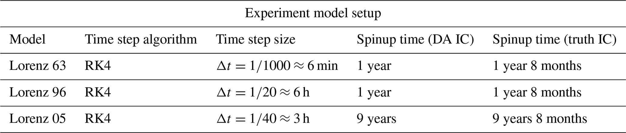
In this section, we will first discuss how the experiments are set up for each of the three models. We will then present results from preliminary testing to establish how the values of the nudging coefficients were chosen for the experiments following. Before performing any experiments, each model requires initialization and a period of forward integration to remove any transient behavior (Lorenz, 2005; Lorenz and Emanuel, 1998), also referred to as the model spinup. Each model follows the experiment setup scheme shown in Fig. 1, and the lengths of time for each model spinup are shown in Table 1.

The models are first initialized with a uniform random distribution between 0 and 1 and integrated forward using a fourth-order Runge–Kutta (RK4) time-stepping algorithm (Lambers et al., 2021), where the size of the time step is model dependent and shown for each model in Table 1. Following the outline in Fig. 1, the model state of the spinup after 1 year (9 years for Lorenz 05) is used as the initial condition for the DA model experiments. The model spinup continues for an additional 8 months to provide an initial condition for the true model. This continued time of spinup is to ensure that the two initial conditions are not equal, which is verified within the following sections. The true model, also referred to as the truth, is integrated forward without any assimilation for a period of 4 months and is used for sampling observations and evaluating the accuracy of the experiments for each DA method.

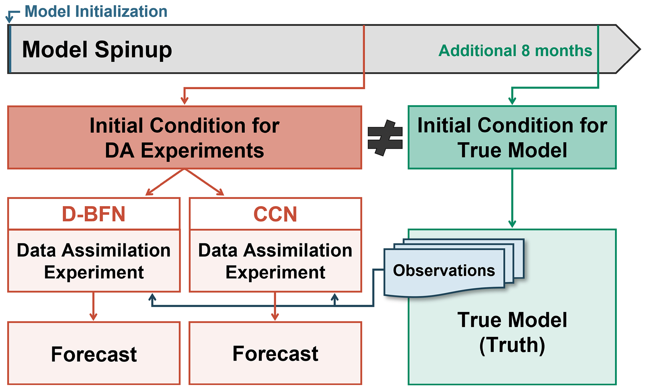
Figure 1 Model initialization and setup for experiments. Note that the initial conditions for the DA experiments and the true model state are not equal. The true model state is also referred to as the truth.

The unit of time used within this paper follows from Lorenz (1996, 2005) and Lorenz and Emanuel (1998), which state that one unit of time is approximately 5 d for the Lorenz 96 and Lorenz 05 models. Lorenz (1963) states that the Lorenz 63 model uses a dimensionless time increment. We note that there are underlying variables within the Lorenz 63 model that can be used to calculate a specific unit of time but are based on values of the materials used within an experiment; an example of this calculation is shown in Ngodock et al. (2009). For the purposes of this paper and to reduce confusion between units of time within the following results, we have made the assumption that a time unit for all three models corresponds to 5 d.

Table 1 Initialization and experiment parameters for each model.

4.1 Lorenz 63 model initialization

The Lorenz 63 model (Eq. 7) is integrated forward, with a time step of approximately 6 min (or $\mathrm{\Delta }t=\mathrm{1}/\mathrm{1000}$ time unit). As shown in Fig. 1 and Table 1, the model state after a 1-year spinup is used as the initial condition for the DA model experiments, and the model state after 1 year and 8 months of the spinup is used as the initial condition for the true model.

First, we verify that the true model, shown in Fig. 2(a), uses an appropriate length of time and produces the rotation between the two wings of the Lorenz attractors. This forecast is referred to as the truth and is used for observation sampling and evaluating the experiments. Next, we note that the two initial conditions $(x,y,z)$ are in fact, not equivalent. The initial condition for the DA experiments was $(\mathrm{2.2731},\mathrm{2.9968},\mathrm{17.2231})$, and the initial condition for the truth was $(\mathrm{-}\mathrm{12.0355},\mathrm{-}\mathrm{15.7630},\mathrm{26.9678})$. Lastly, we validate that the forecasts produced by these two initial conditions do not converge. The 2-month forecasts with no assimilation are shown in Fig. 2b for each variable, x (top), y (middle), and z (bottom).

Figure 2 Lorenz 63 model. (a) The 4-month forecast of the true model, referred to as the truth. (b) The 2-month forecasts with no assimilation for each variable x (top), y (middle), and z (bottom). The teal line shows the truth, “true FC”, or the forecast using the initial condition for the true model, whereas the orange line shows the no-assimilation forecast using the initial condition for the DA experiments, “no DA FC”.

4.2 Lorenz 96 model initialization

The Lorenz 96 model (Eq. 8) uses a constant forcing of F=8 and is integrated forward using a 6 h time step (or $\mathrm{\Delta }t=\mathrm{1}/\mathrm{20}$ time unit). The model setup is parallel to the previous model, as shown in Fig. 1, where the model state after a 1-year spinup is used as the initial condition for the DA experiments, and the model state after 1 year and 8 months of the spinup is used as the initial condition for the true model.

These initial conditions are presented in Fig. 3a to confirm that they are different. Figure 3b shows the 4-month forecast for the true model, referred to as the truth, and verifies the length of spinup and choice of forcing produced a chaotic system. The truth is used for sampling observations and validating results from the experiments. Lastly, we validate that the initial conditions produce separate forecasts. Figure 3c represents the error between the truth and the no-assimilation forecast using the initial condition for the DA experiments. The magnitude of the errors verifies that the two forecasts do not converge.

Figure 3 Lorenz 96 model. (a) The teal line shows the initial condition for the true model state, “truth IC”, whereas the orange line shows the initial condition for the DA experiments, “DA IC”. (b) The 4-month forecast of the true model, referred to as the truth. (c) Difference between a 4-month no-assimilation forecast of the DA IC and the truth.

4.3 Lorenz 2005 model initialization

The Lorenz 05 model (Eqs. 9 and 10) uses a constant forcing of F=10 to ensure chaos and an even number L=8 and is integrated forward with a time step of approximately 3 h (or $\mathrm{\Delta }t=\mathrm{1}/\mathrm{40}$ time unit). This model setup is similar to the previous two models with the exception of the length of time for the model spinup. Table 1 and Fig. 1 show this model has a 9-year spinup, where the final model state is used as the initial condition for the DA experiments. The spinup continues for an additional 8 months to provide the initial condition for the true model which is the final model state of the spinup after 9 years and 8 months.

These initial conditions are not equal and are shown in Fig. 4a. A 4-month forecast of the true model is shown in Fig. 4b, which validates the choice of forcing term and confirms that the length of spinup removed any transient effects. This forecast is referred to as the truth and is used for sampling observations and evaluating the results between the two methods. Finally, we present the error between the true model forecast and a no-assimilation forecast of the initial condition for the DA experiments in Fig. 4c, which verifies that the two initial conditions do not converge.

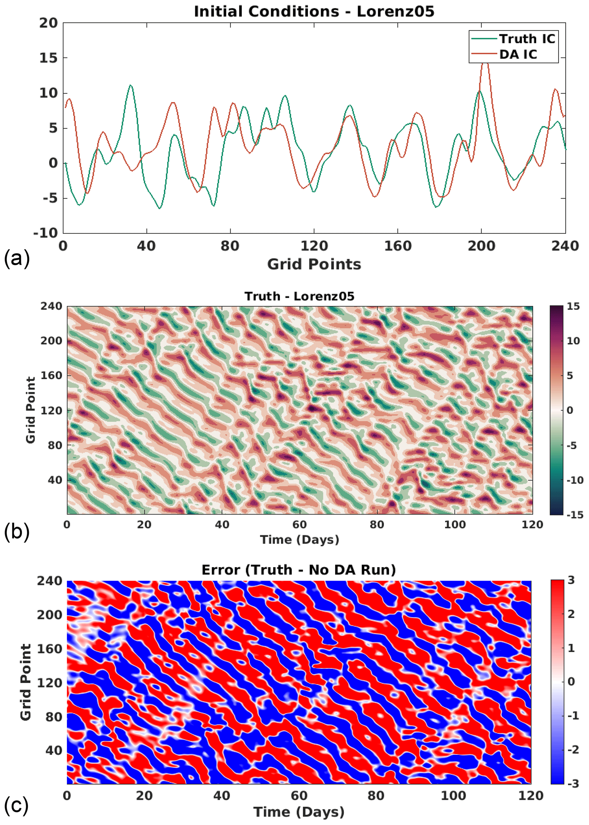
Figure 4 Lorenz 05 model. (a) The teal line shows the initial condition for the true model state, truth IC, whereas the orange line shows the initial condition for the DA experiments, DA IC. (b) The 4-month forecast of the true model, referred to as the truth. (c) Difference between a 4-month no-assimilation forecast of the DA IC and the truth.

4.4 Preliminary testing

In order to best compare the two methods, we first completed preliminary testing to choose a value for the nudging coefficients for each model. The two DA methods, D-BFN and CCN, were implemented for several lengths of time, ranging from 5 d to 2 months. Each experiment was given a set of full observations at all grid points and every time step. The mean absolute error (MAE; $\frac{\mathrm{1}}{N}{\sum }_{i=\mathrm{1}}^N|y_i-x_i|$) was computed over time to reflect how well the nudging terms were correcting the models. Several values were tested for each nudging term: $\mathrm{1}\le \left|K\right|\le \mathrm{75}$ and $\mathrm{0}<\mathit{\gamma }<\mathrm{1}$.

While we evaluated this preliminary testing for each model and a range of parameters, we only present the two examples shown in Fig. 5 so as to not cloud the paper with repetitive figures. The results shown are the errors as the Lorenz 05 model assimilates all observations over a 1-month period. Figure 5a represents the error for D-BFN over three iterations of back-and-forth nudging, where the value K=25 maintained the lowest overall error. Figure 5b shows the error for CCN where the value γ=0.9 reduces and maintains this lower error around day 10.

We remind the readers that CCN is a continuous method that corrects through forward integration only, which explains why this method will have higher errors at the beginning of the window and might need a longer time to reduce the error. Similar results were obtained for each model in our preliminary testing, and so we proceed with using the values K=25 for D-BFN and γ=0.9 for CCN for the following experiments and their results shown in this paper.

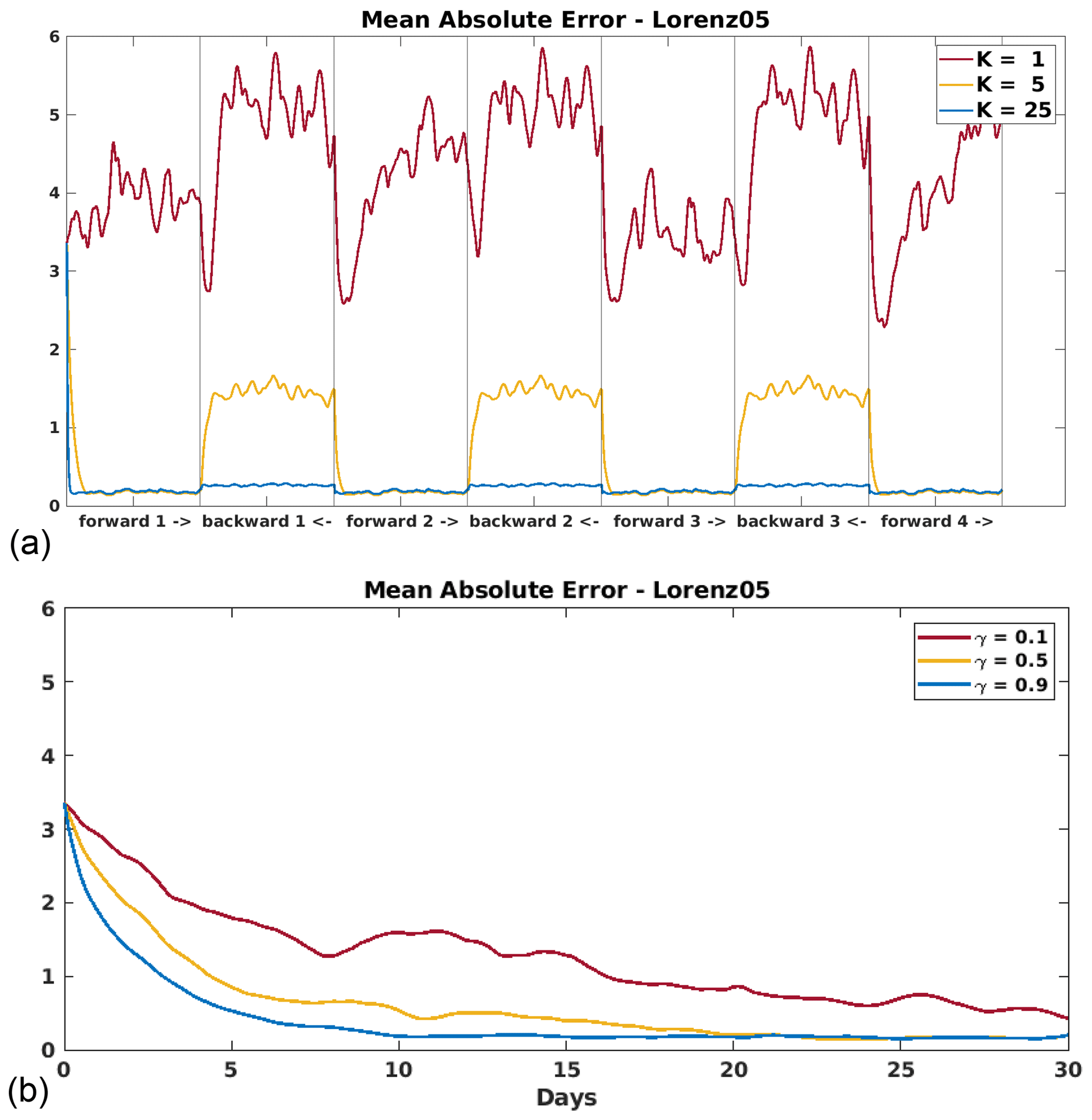
Figure 5 Preliminary testing results of the Lorenz 05 model that assimilated 1 month of full observations for (a) D-BFN with the values K=1, 5, and 25 and (b) CCN with the values γ=0.1, 0.5, and 0.9.

5 Data assimilation experiments: setup and results

For each model subsection, we start with briefly discussing the individual model parameters used for the following experiments. We then proceed with details of the DA experiments, such as the length of the DA period and the frequency in which observations are assimilated, and discuss the results shown in the tables and figures presented for each model.

Within this section, several experiments are carried out with different lengths of DA experiment periods. Each forecast is presented for the same length of time as the corresponding DA experiment window. The observations assimilated in these experiments are sampled from the truth for each model. We remind the reader of the results from the preliminary testing in the previous section, where the values K=25 for D-BFN and γ=0.9 for CCN are used for all results shown in this study.

The first set of experiments for each model assimilates observations at all grid points for every time step and is referred to as the “ALL OBS” experiments. The tables presented within this section include shorthand names for other experiments, where the first number represents the spacing between grid points and the second number represents the time between time steps. For example, the experiment “3GP-2TS” assimilated observations at every three grid points for every two time steps. The results shown in the tables are the mean absolute error (MAE) averaged over time. The columns separate the errors between the DA experiment periods and the forecast periods.

The results shown in the figures within this section contain the errors for each DA experiment evaluated against the truth and are presented in the following manner:

• i.

  Experiment results for D-BFN are presented in the top row of each figure (panels a and c), while experiment results for CCN are presented in the bottom row of each figure (panels b and d).

• ii.

  The error for the DA experiment period is shown in the left half of the panel, while the error of the forecast (FC) is shown in the right half of the panel. This distinction is shown by color in the results for Lorenz 63 and is separated by a vertical line for all remaining figures.

5.1 Lorenz 63 model

The first set of experiments is carried out with the three-component Lorenz 63 model (Eq. 7). All experiments have the same parameters of $\mathit{\sigma }=\mathrm{10},\mathit{\beta }=\frac{\mathrm{8}}{\mathrm{3}}$, and ρ=28 with a time step of approximately 6 min $(\mathrm{\Delta }t=\mathrm{1}/\mathrm{1000})$.

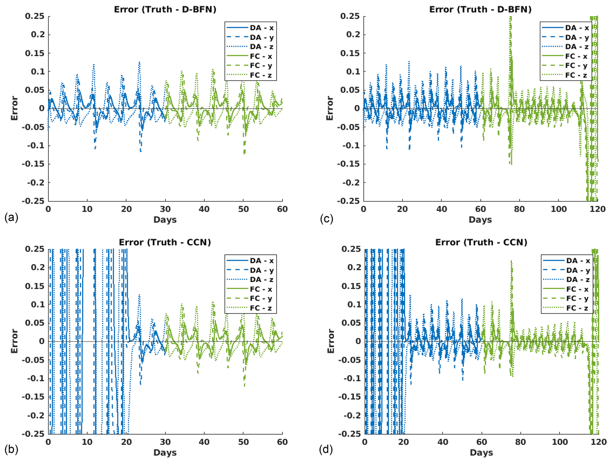
Figure 6 Error plots for Lorenz 63 ALL OBS experiments evaluated against the truth for each variable, x (solid line), y (dashed line), and z (dotted line). Blue denotes the DA error, while green denotes the FC error. The left column (a, b) shows results for 1-month DA and 1-month FC for (a) D-BFN and (b) CCN. The right column (c, d) shows results for 2-month DA and 2-month FC for (c) D-BFN and (d) CCN.

The first setup starts with shorter DA experiment periods of 5 and 10 d, paired with their 5 and 10 d forecasts, respectively. For the best results possible, observations were brought in at all grid points for every time step (ALL OBS). Table 2 shows the MAE of the DA period and the forecast period (FC) for both methods, D-BFN and CCN. While D-BFN does well with a short experiment window, CCN does not have an adequate amount of time for corrections to make an impact on the DA error.

The experiment window was then extended to 1 and 2 months for the DA period and FC period. The results are shown in Table 2, as well as Fig. 6. While CCN shows higher MAE for not having a long enough time window to reduce errors, the forecast MAE is on par with D-BFN for the 1-month forecast and slightly better than D-BFN for the 2-month forecast. Figure 6c and d show that CCN has better accuracy in the forecast for several days longer than D-BFN when given sufficient time to make corrections.

Further experiments were done in the case when all observations are not available. The “1GP-2TS” experiment shown in Table 2 brings in observations at all grid points but now every other time step. These were only performed for the longer experiment windows of 1 and 2 months. D-BFN still provided high accuracy with fewer observations in time, but CCN was not able to make a suitable correction within this time window. Several factors play a role in this outcome starting with internal factors of D-BFN, namely the backwards integration of the model and the iterations. The backwards integration helps propagate the correction from the nudging term further into the model domain, an ability that is not present in CCN. It can also be seen in Fig. 5 that the rate in which corrections are made imply that D-BFN has a stronger nudging term compared to CCN. It is possible that if a longer time window were considered, CCN would produce lower errors for the DA run and the forecast. It was shown in the original paper that it took approximately 17 time units to converge with the Kuramoto–Sivashinsky equation, and these experiments are 6 time units (1 month) and 12 time units (2 months).

Table 2 Table of DA experiments. Observations used are as follows: ALL OBS is all observations (every 6 min), and 1GP-2TS is all grid points, every other time step (every 12 min). 1m and 2m represent 1 month and 2 months, respectively. DA is the experiment window for data assimilation, and FC is the forecast window. Values shown are the MAE.

Table 3 Table of DA experiments. Observations used are as follows: ALL OBS is all observations (every 6 h), and 1GP-2TS is all grid points, every other time step (every 12 h). 1m and 2m represent 1 month and 2 months, respectively. DA is the window for data assimilation, and FC is the forecast window. Values shown are the time-averaged MAE.

Figure 7 Error plots for Lorenz 96 ALL OBS experiments evaluated against the truth. The left column (a, b) shows results for 1-month DA and 1-month FC for (a) D-BFN and (b) CCN. The right column (c, d) shows results for 2-month DA and 2-month FC for (c) D-BFN and (d) CCN.

The results above confirmed that a longer time window is still needed with these models in order for CCN to converge. Therefore, the next two models will only use the longer experiment window. For the following experiments, the two lengths of assimilation considered are 1 and 2 months followed by their respective forecast.

5.2 Lorenz 96 model

All numerical experiments for Lorenz 96 (Eq. 8) use the following parameters: N=40 grid points, F=8, and a time step of approximately 6 h $(\mathrm{\Delta }t=\mathrm{1}/\mathrm{20})$.

The first set of experiments with this model uses observations at all grid points and all time steps (ALL OBS). The time-averaged MAE is shown in Table 3; CCN produces a slightly better forecast than D-BFN. Of course, CCN has a higher error for DA since it only corrects in the forward model. Figure 7a and c show how long the forecast is accurate for the 1-month experiment, which is around 12–15 d for both methods. Figure 7c and d contain the results for the 2-month experiment, showing that the accuracy in the forecast for D-BFN has decreased to around 5 d, whereas CCN is consistent in accuracy for about 12–15 d.

The next set of experiments brought in observations at all grid points and every other time step (1GP-2TS). Figure 8 shows the error between the truth and each method along with their forecast. D-BFN produces similar results as compared to assimilating all observations. CCN, however, does not make much of a correction during assimilation, which in return does not produce a usable forecast. We would hypothesize that CCN needs a much longer assimilation window to account for not having a full observation set. We carried out experiments with smaller and slightly higher values for γ, but the resulting assimilation and forecast errors did not improve (results not shown).

Figure 8 Error plots for Lorenz 96 1GP-2TS experiments evaluated against the truth. The left column (a, b) shows results for 1-month DA and 1-month FC for (a) D-BFN and (b) CCN. The right column (c, d) shows results for 2-month DA and 2-month FC for (c) D-BFN and (d) CCN.

Table 4 A variety of other experiments testing the sparsity of observations. The first number represents the spacing between grid points, whereas the second represents the time between time steps. For example, 3GP-2TS denotes observations brought in at every three grid points and every two time steps. Recall that one time step is equal to 6 h for this model, so every two time steps would be every 12 h. Values shown are the time-averaged MAE.

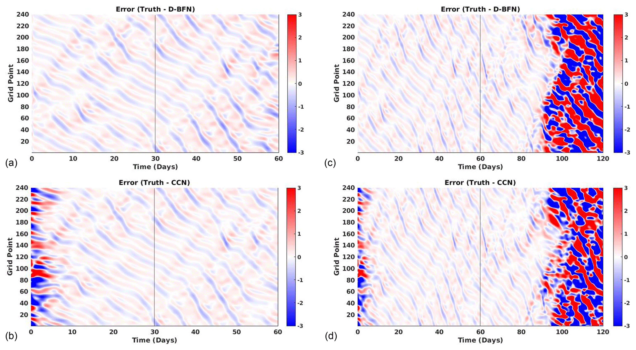
Figure 9 Error plots for Lorenz 05 ALL OBS experiments evaluated against the truth. The left column (a, b) shows results for 1-month DA and 1-month FC for (a) D-BFN and (b) CCN. The right column (c, d) shows results for 2-month DA and 2-month FC for (c) D-BFN and (d) CCN.

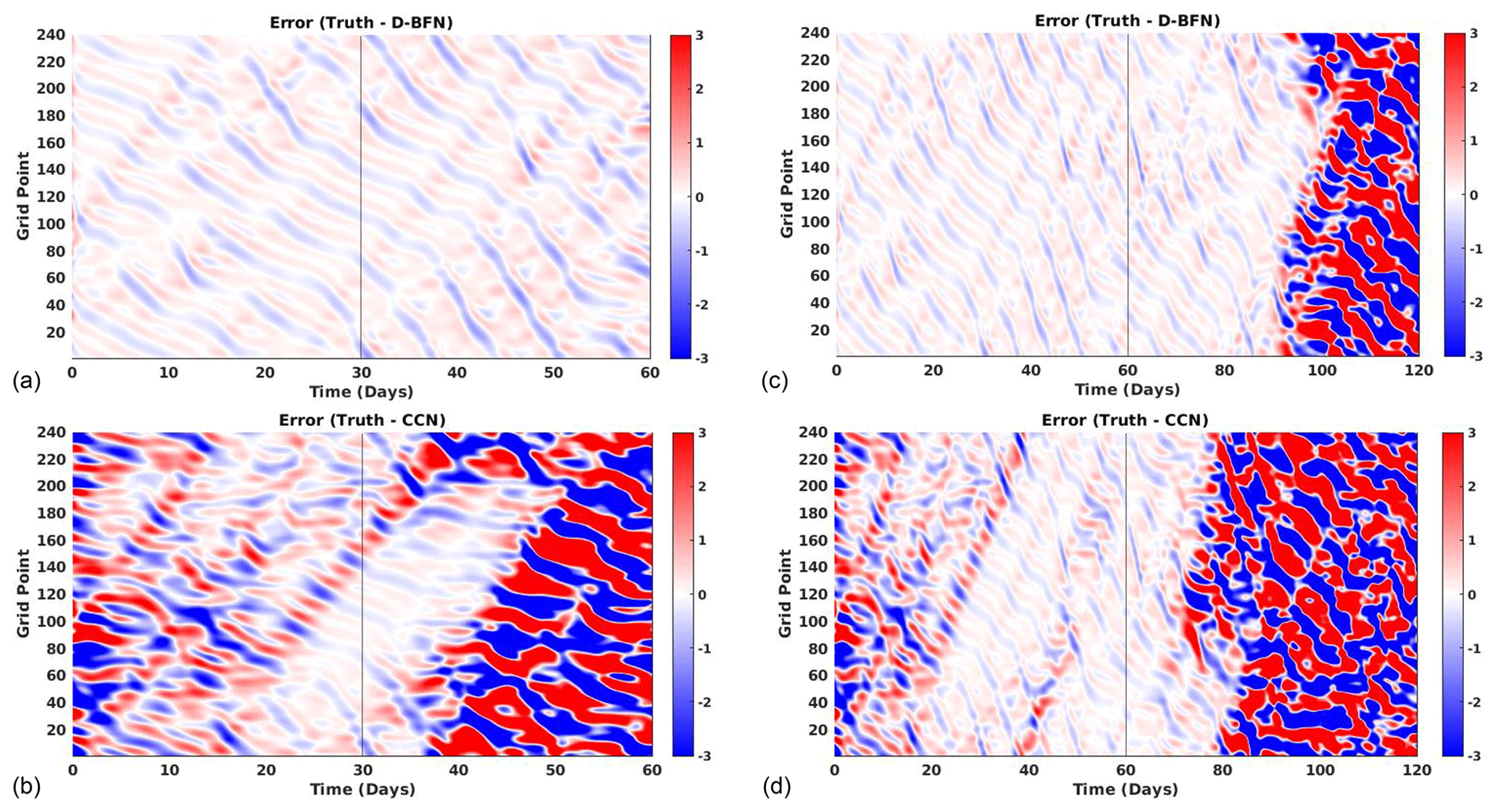
Figure 10 Error plots for Lorenz 05 1GP-2TS experiments evaluated against the truth. The left column (a, b) shows results for 1-month DA and 1-month FC for (a) D-BFN and (b) CCN. The right column (c, d) shows results for 2-month DA and 2-month FC for (c) D-BFN and (d) CCN.

Table 5 Table of DA experiments. Observations used are as follows: ALL OBS is all observations (every 3 h), and 1GP-2TS is all grid points, every other time step (every 6 h). 1m and 2m represent 1 month and 2 months, respectively. DA is the window for data assimilation, and FC is the forecast window. Values shown are the time-averaged MAE.

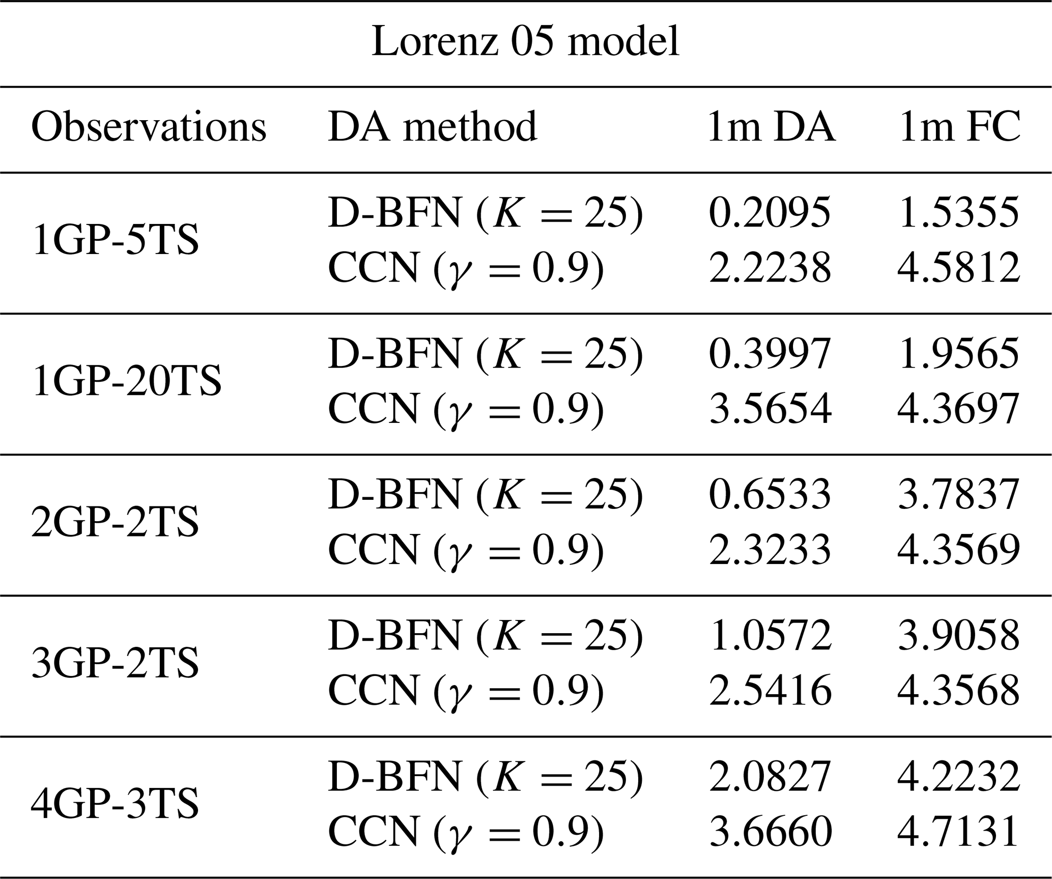
Table 6 A variety of other experiments testing the sparsity of observations. The first number represents the spacing between grid points, whereas the second represents the time between time steps. For example, 3GP-2TS denotes observations brought in at every three grid points and every two time steps. Recall that one time step is equal to 6 h for this model, so every two time steps would be every 12 h. Values shown are the time-averaged MAE.

A few other experiments were performed to test the capabilities of these methods with sparse observations. All of these were completed with the 2-month experiment window. Observations were assimilated less frequently in time, from every 5 (“1GP-5TS”) to every 10 (“1GP-10TS”) to every 20 (“1GP-20TS”) time steps. The results are displayed in Table 4. The results for CCN are poor as it did not have enough observations to make a correction in the forward model. D-BFN has the benefit of propagating the observations back in time, correcting the initial conditions, and running the forward model again. This process allows D-BFN to give a much better correction during the assimilation window. However, the forecast accuracy decreases with the frequency of observations. The results for every five time steps (every 30 h) are comparable to the results from all observations. The number of days of accuracy for the less frequent observations drastically decreases as the number of observations decreases.

5.3 Lorenz 2005 model

The Lorenz 05 model (Eqs. 9 and 10) use the same parameters for all numerical experiments: 240 grid points (N), an even number L=8, a forcing constant of 15 to ensure chaos (F), and a time step of approximately 3 h ($\mathrm{\Delta }t=\mathrm{1}/\mathrm{40}$ time unit). Recall that in Eqs. (9) and (10), one unit of time is equivalent to 5 d.

The first set of experiments with this model uses observations at all times and space (ALL OBS) for 1- and 2-month experiment windows. For this model, CCN has the lowest forecast accuracy of all results for both the 1-month and 2-month experiments. The forecast has high accuracy for around 30 d, as seen in Fig. 9.

The second set of experiments uses all points in space and assimilates them at every other time step (1GP-2TS). D-BFN produces very similar results to those from the ALL OBS experiment. Looking at the difference in results between the 1-month and 2-month experiments, the CCN method needs a longer window to converge with the sparser set of observations, as seen in Fig. 10. Table 5 contains further details of the time-averaged MAE for the first two sets of experiments. The values in Table 5 are separated to show error contained during the DA period and error maintained during the forecast period.

D-BFN does well compared to CCN for observations that are sparse in time. Table 6 shows the results for the 2-month DA and FC experiments for observations brought in every 5 (1GP-5TS) and every 20 (1GP-20TS) time steps. The correction in the DA brings the error down to provide a decent forecast. The error in the forecast is relatively low compared to the errors in CCN, and the larger errors are towards the end of the forecast period. The figure is not shown in this paper, but both results have high accuracy for approximately the first 30 d of the forecast.

6 Conclusions

Overall, each method has their own advantages and disadvantages. While D-BFN performs better with short windows and sparse observations, it does require iterations of forward and backward integrations of the model. This is not suitable for all cases, most importantly when a model cannot be integrated backwards. For some cases where the assimilation window was long enough, the DA error at the end of the window was lower from the CCN method than D-BFN, resulting in a forecast that maintained accuracy longer in time. Furthermore, CCN only requires the forward model, which is useful for models that do not allow for a backwards integration and also makes this method more computationally efficient.

We want to remember that a goal of this paper was to determine the best method to apply to an ocean model. For this reason, we do not want to implement a longer time window as it is not practical for ocean DA. In terms of implementing either method for an ocean model, based on the findings in this paper, Auroux and Blum's D-BFN method seems more applicable to the assimilation window constraints and sparse ocean observations available. However, the implementation of CCN may be suitable for other scenarios with a long assimilation in the ocean such as that done in reanalysis or assimilations that start much further in the past.

The results from this paper led us to the conclusions above, but we leave the reader with this final remark. While D-BFN is able to retain accuracy for observations that are sparse in time, due to the advantage of spreading these corrections through the back-and-forth iterations, we observed that the results from CCN decayed as the density and/or frequency of observations was reduced. These results may partially be due to the models not having strong dynamics capable of propagating the corrections to other unobserved points in space or time. However, for models with strong advection, the corrected term may be able to disperse these corrections to places where observations are not observed, which would allow CCN to have a higher impact when adjusting the trajectory from sparse observations.