The role of time-varying external factors in the intensification of tropical cyclones

The role of time-varying external parameters in tropical cyclone (TC) dynamics is explored through a low-order conceptual box model. Specifically, we look at stable-to-stable state transitions which may be linked to tropical cyclone intensification, dissipation, or eyewall replacement cycles (ERCs). To this end, we identify two parameters of interest: the exponent of radial decline and sea-surface temperature. We examine how variations in these parameters affect the stable states of the model and consider the behaviour of the system under different time-dependent forcing profiles for the parameters. By externally forcing the exponent of radial decline and sea-surface temperature, we show the existence of rate-dependent behaviour in the model. These findings are brought together in a case study of Hurricane Irma (2017). The results highlight the role of the radial vorticity gradient in behaviour such as rate-induced tipping and overshoot recovery. They also show that a simple model can be used to explore relatively complex tropical cyclone dynamics.

1 Introduction

Rapidly rotating storm systems, commonly called tropical cyclones (TCs), are one of the most iconic yet destructive atmospheric phenomena. It is estimated that the damage from TCs has resulted in an average cost of USD 51.5 billion over the last decade (Krichene et al., 2023). Improvements in our ability to accurately model and predict their behaviour will result in the saving of lives and infrastructure. In the last 50 years, much work has been done to develop systems of equations which describe the fluid mechanical and thermodynamic evolution of TC systems, e.g. Anthes (1982) and Emanuel (1988). More recently, such systems have been adapted for analysis within a dynamical system framework, which has helped to extend our understanding of the qualitative nature of TCs, e.g. Schönemann and Frisius (2012) and Slyman et al. (2024). Here, we use a dynamical system directly derived from the first principles of physics to explore the role of the radial vorticity gradient and sea-surface temperature in TC intensification and dissipation. We connect our findings to the dynamics of eyewall replacement cycles through the identification of relevant parameters and transient changes to the radial extent of the eyewall.

1.1 Vorticity, intensification, and eyewall replacement cycles

The circulation of a TC is initiated by combined vorticity effects in the atmosphere. This vorticity is composed of both the ambient vorticity due to the Earth's rotation, given by the Coriolis parameter, and the relative vorticity of the atmospheric flow. Weak vertical wind shear is also necessary so that a developing TC does not break apart as its convection grows through the layers of the atmosphere (Gray, 1998). Once initiated, TCs are maintained by convection within the eyewall; thus, they require a constant heat source. This heat is mainly provided through heat exchange between the ocean surface and the boundary-layer flow. The observationally derived critical SST temperature for TC formation is 26.5 °C; below this threshold, TCs are not observed to form (Anthes, 1982).

An important phenomenon which can occur within TCs is the eyewall replacement cycle (ERC), where a secondary tangential wind maximum forms outside the primary eyewall. As this secondary eyewall forms, it is theorised that its convection consumes an increasing proportion of the radial inflow, effectively “choking” the inner eyewall (Kepert, 2013). As the inner eyewall dissipates, the secondary eyewall contracts and intensifies. The sequence generally occurs over a 12 to 36 h period and can repeat multiple times throughout the lifespan of the TC (Sitkowski et al., 2011). An ERC can impact TC forecasting as it causes the intensity of the TC to fluctuate dramatically. If the wind speed of the inner eyewall is used to measure the strength of a TC, an ERC may be mistaken for the dissipation of the TC.

ERCs were first observed to occur within Typhoon Sarah, which moved through the northern Pacific in 1956 (Fortner, 1958). As observation techniques progressed, ERCs were found to be a common feature of TCs (Sitkowski et al., 2011). A recent example is the ERCs observed within Hurricane Irma, which formed in the North Atlantic in 2017 (Fischer et al., 2020). Two ERCs were observed, with each taking place over less than 12 h. Interestingly, the first ERC consisted of inner eyewall weakening and dissipation, as expected, but the second ERC resulted in a continual rapid intensification (RI) of the TC (Fischer et al., 2020). This behaviour contradicts the common model of ERCs and shows that there is still much work to be done in understanding this phenomenon.

By converging air and thus energy to the TC centre, the boundary layer plays an important role in intensity changes such as intensification or secondary eyewall formation. Frictional updraft plays a major role in driving convection within the eyewall and begins within the boundary layer (Kepert, 2013). Thus, changes to boundary-layer parameters linked to frictional updraft may lead to the strengthening or initiation of deep convection. Boundary-layer parameters which have been proposed to directly affect convection within the eyewall are the inflow rate, the tangential and gradient wind maxima, and the radial vorticity gradient (Kepert, 2013). Further, it has been theorised that the frictionally forced vertical velocity at an eyewall is approximately proportional to the radial vorticity gradient (Kepert, 2013). In light of the model used in this study, we focus here on the closely related roles of the radial vorticity gradient and the inflow rate. If we consider an increase in the radial vorticity gradient, this implies an increase in the radial wind shear, i.e. a greater tangential wind gradient. An increase in the tangential wind gradient can be explained by increased tangential wind speed within the eyewall, which implies that the total energy of the TC has increased. An energy increase necessitates that energy transportation via the boundary-layer flow increases, which can be realised by an increase in the radial inflow (Anthes, 1982). The relation can be framed in the opposite direction as it is not known that one change necessarily precedes the other.

Multiple studies have supported this theory regarding the connection between the radial vorticity gradient and TC intensification. In a study of TC development, Ge et al. (2015) found that the radial profile of the inner-core relative vorticity was important in determining the strength and success of initial TC intensification. They compared two vortex models with different inner-core structures and found that the vortex with a “higher inner-core vorticity and larger negative radial vorticity gradient” promoted the formation of small-scale convective cells which act to intensify the TC. Additionally, in an analysis of three TC boundary-layer models, Kepert (2013) found that a “relatively weak local enhancement” of the radial vorticity gradient outside of the eyewall can produce a frictional updraft of the strength necessary for initiation of a secondary eyewall. He also found that once a secondary eyewall formed, it possessed significantly stronger frictional updraft than the inner eyewall due to its position within a lower-vorticity environment.

1.2 Rate-induced dynamics

There are multiple mechanisms which can cause a system to transition between stable states. The most widely known and studied are bifurcation-induced transitions (or B-tipping). These occur when external forcing causes a system to cross a bifurcation (a point of change in local stability). Once the bifurcation point has been crossed, the stable state which the system had previously been tracking disappears; thus, it must transition to a new stable state (assuming one exists).

Another, more recently discovered, mechanism for transitions is rate-induced transitions (or R-tipping) (Ashwin et al., 2012). These transitions occur without the crossing of a bifurcation point and are instead a result of the rate at which a parameter is externally forced. When the rate of change in the external forcing profile is greater than some critical value, the system becomes unable to track its original stable state. Tipping occurs when the system moves too far from the stable state and crosses some threshold. These rate-dependent behaviours have been shown to exist in conceptual models of geophysical systems such as the Indian summer monsoon (Ritchie et al., 2019) and, more recently, TC formation (Slyman et al., 2024). As TCs experience changing environmental conditions throughout their lifetime, rate-dependent behaviours can be expected to play a role in TC intensification as well.

To define the rate of external forcing, we follow Ritchie et al. (2023) and define an external forcing parameter, σ≡σ(λt), where u=λt is dimensionless. The rate parameter, λ, is in units of per second, day, year, etc. depending on the application. It is useful to note that the rate of change in the external forcing parameter and the rate parameter are related by

$$\begin{array}{}\text{(1)}& {\displaystyle \frac{\mathrm{d}\mathit{\sigma }}{\mathrm{d}t}}={\displaystyle \frac{\mathrm{d}\mathit{\sigma }}{\mathrm{d}u}}{\displaystyle \frac{\mathrm{d}u}{\mathrm{d}t}}=\mathit{\lambda }{\displaystyle \frac{\mathrm{d}\mathit{\sigma }\left(u\right)}{\mathrm{d}u}},\end{array}$$

which has units of σ per second, day, year, etc. and depends on λ and σ(u) itself (Ritchie et al., 2023). So, for a fixed forcing profile, σ(u), λ quantifies the rate of change in this profile. The critical rate is then the value of λ at which rate-induced tipping occurs, assuming the magnitude of the parameter shift remains the same.

A phenomenon closely related to rate-induced tipping is the overshooting of a bifurcation point without tipping, sometimes referred to as “return tipping” (Ritchie et al., 2023). In this case, the system is externally forced across a bifurcation but may avoid tipping and recover its original state if the reversal in the forcing is faster than some critical rate.

2 A low-order model

This analysis uses a low-order box model derived from geophysical principles as presented by Schönemann and Frisius (2012) (S&F). The model uses cylindrical coordinates and assumes an axisymmetric TC; thus, it only considers variation in the radial (r) and vertical (z) directions. It assumes a length scale over which variation in the Coriolis parameter is negligible and thus takes it to be constant (f-plane approximation). It also applies both Boussinesq and hydrostatic approximations to the governing fluid equations. The model considers three regions situated on top of a boundary layer: the eye, eyewall, and ambient region. A sketch of this division is shown in Fig. 1. The boundaries between these regions are defined by lines of constant potential radius. The potential radius is the physical radius to which a particle must be moved whilst conserving absolute angular momentum in order to bring its relative angular momentum to zero. The S&F model takes the potential radius to be defined as

$$\begin{array}{}\text{(2)}& R=\sqrt{r^{\mathrm{2}}+{\displaystyle \frac{\mathrm{2}vr}{f}}}=\sqrt{{\displaystyle \frac{\mathrm{2}m}{f}}}.\end{array}$$

Here, v is the tangential wind velocity, f the Coriolis parameter, and m the angular momentum per unit mass. Hence, lines of constant potential radius correspond to lines of constant angular momentum or “angular momentum surfaces” in three dimensions.

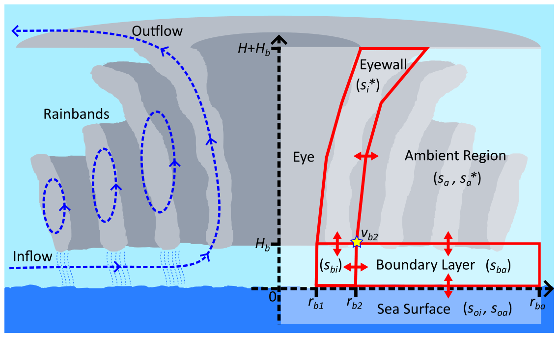
Figure 1 An idealised cross section of a TC with the box model overlaid (red). Here, H_b is the boundary-layer height, H the tropopause height, s the specific entropy, and r the physical radius in the boundary layer. The subscripts i, b, and a denote the inner eyewall, boundary layer, and ambient region, respectively. The symbol * denotes a variable at saturation.

The S&F model consists of a system of three first-order non-linear differential equations which model the change in entropy within the important TC regions. In attempting to simulate the model, we found inconsistencies in the timescales as written in the original paper. After conducting a thorough scale analysis we amended the model as follows:

$$\begin{array}{}\text{(3a)}& {\displaystyle \frac{\mathrm{d}{s}_{\mathrm{i}}^{*}}{\mathrm{d}t}}=A\left({\mathrm{\Psi }}_{\mathrm{b}\mathrm{2}}\left(s_{\mathrm{i}}^{*}\right){\displaystyle \frac{s_{\mathrm{bi}}-s_{\mathrm{i}}^{*}}{M_{\mathrm{i}}}}\right)+{\displaystyle \frac{s_{\mathrm{a}}^{*}-s_{\mathrm{i}}^{*}}{{\mathit{\tau }}_E}},\text{(3b)}& {\displaystyle }\begin{array}{rl}{\displaystyle \frac{\mathrm{d}{s}_{\mathrm{bi}}}{\mathrm{d}t}}& =A\left({\mathrm{\Psi }}_{\mathrm{b}\mathrm{2}}\left(s_{\mathrm{i}}^{*}\right){\displaystyle \frac{s_{\mathrm{ba}}-s_{\mathrm{bi}}}{M_{\mathrm{bi}}\left(s_{\mathrm{i}}^{*}\right)}}+{\displaystyle \frac{C_H}{\mathrm{2}{H}_{\mathrm{b}}}}\left(\left|v_{\mathrm{b}\mathrm{1}}\right(s_{\mathrm{i}}^{*})\right.\right.\\ & \left.\left.|+|v_{\mathrm{b}\mathrm{2}}\left(s_{\mathrm{i}}^{*}\right)|\right)\left(s_{\mathrm{oi}}\left(s_{\mathrm{i}}^{*}\right)-s_{\mathrm{bi}}\right)\right),\end{array}\text{(3c)}& {\displaystyle }\begin{array}{rl}{\displaystyle \frac{\mathrm{d}{s}_{\mathrm{ba}}}{\mathrm{d}t}}& =A\left({\mathrm{\Psi }}_{\mathrm{b}\mathrm{2}}\left(s_{\mathrm{i}}^{*}\right){\displaystyle \frac{\mathit{\delta }{s}_{\mathrm{a}}-s_{\mathrm{ba}}}{M_{\mathrm{ba}}\left(s_{\mathrm{i}}^{*}\right)}}+{\displaystyle \frac{C_H}{\mathrm{2}{H}_{\mathrm{b}}}}\left|v_{\mathrm{b}\mathrm{2}}\right(s_{\mathrm{i}}^{*}\left)\right|\left(s_{\mathrm{oa}}\left(s_{\mathrm{i}}^{*}\right)\right.\right.\\ & \left.\left.-s_{\mathrm{ba}}\right)\right)+{\displaystyle \frac{s_{\mathrm{a}}-s_{\mathrm{ba}}}{{\mathit{\tau }}_C}},\end{array}\end{array}$$

where A is the added rescale factor and set to A=3600. Here, * denotes a variable at saturation. We have the dependent entropy variables that correspond to different regions of the model: $s_{\mathrm{i}}^{*}$ is the eyewall saturated specific entropy, s_bi is the eyewall boundary-layer specific entropy, and s_ba is the boundary-layer specific entropy in the ambient region. The remaining entropy variables are as follows: $s_{\mathrm{a}}^{*}$ is the saturated specific entropy in the ambient region, s_oi is the sea-surface specific entropy under the eyewall, and s_oa is the sea-surface specific entropy in the ambient region. These are either constants or functions of the dependent variables. It is important to note that these entropy variables measure the perturbation from the mean atmospheric entropy and are not a total entropy measure. From here on, “entropy” refers to specific entropy. The mass-stream function, Ψ₂, is responsible for mass exchange between regions. The region masses, M, with corresponding subscripts denote the mass enclosed by each region. We then have the constants H_b – the height of the boundary layer, τ_E – the timescale of diabatic cooling, τ_C – the timescale of convective exchange, δ – the entrainment parameter (a proxy for the effects of wind shear), and C_H – the transfer coefficient for enthalpy. The tangential velocities v are taken at the inner (b1) and outer (b2) edges of the eyewall boundary layer. An outline of the auxiliary equations is provided in Appendix A1.

As a brief overview, for the change in eyewall entropy (Eq. 3a), the first term on the RHS gives the vertical transport of entropy from the eyewall boundary layer into the eyewall. The second term gives the change due to diabatic cooling (heat exchange) between the eyewall and ambient region. For the change in eyewall boundary-layer entropy (Eq. 3b), the first term gives the advective transport of entropy within the boundary layer, i.e. the horizontal transport from the boundary layer in the ambient region into the eyewall boundary layer. The second term gives the surface transfer of latent heat from the sea surface into the eyewall boundary layer. For the change in boundary-layer entropy in the ambient region (Eq. 3c), the first term gives the vertical transport of entropy from the ambient region into the boundary layer in the ambient region. The second term gives the surface transfer of latent heat from the sea surface into the boundary layer in the ambient region. The third term gives the entropy exchange due to shallow convection between the ambient and ambient boundary-layer regions.

In this study, we scale Eq. (3) to evolve on a timescale similar to that observed for the phenomena we are interested in. In the case of intensification due to ERCs, we are interested in timescales of 10–20 h. Via experimentation, we scale Eq. (3) by a factor of 40. The constant parameter values used in this study are those given by S&F (Schönemann and Frisius, 2012) and are provided in Appendix A2.

In a physical context, we are interested in the maximum wind speed a TC produces; thus, here we present only the resulting tangential wind speed taken at the outer eyewall boundary, denoted by v_b2. This wind speed is given as

$$\begin{array}{}\text{(4)}& v_{\mathrm{b}\mathrm{2}}={\displaystyle \frac{f}{\mathrm{2}}}\left({\displaystyle \frac{R_{\mathrm{2}}^{\mathrm{2}}-r_{\mathrm{b}\mathrm{2}}^{\mathrm{2}}}{r_{\mathrm{b}\mathrm{2}}}}\right),\end{array}$$

where R₂ and r_b2 are taken at the outer eyewall boundary. As only this maximum speed at the outer eyewall boundary is being considered, an ERC for this model can be deduced from an increase in r_b2 (as well as v_b2) rather than the existence of multiple tangential wind maxima.

To quantify changes to the radial vorticity gradient, we first consider the absolute vorticity in the boundary layer, ζ_b, which is composed of the ambient vorticity due to the rotation of the Earth (f) and the relative vorticity of the fluid flow itself, given as

$$\begin{array}{}\text{(5)}& {\mathit{\zeta }}_{\mathrm{b}}=f+{\displaystyle \frac{v_{\mathrm{b}}}{r_{\mathrm{b}}}}+{\displaystyle \frac{\partial v_{\mathrm{b}}}{\partial r_{\mathrm{b}}}}.\end{array}$$

To determine the absolute vorticity at the outer eyewall boundary (ζ_b2), a tangential wind profile (in the radial direction) for that region is needed. The model assumes a profile of

$$\begin{array}{}\text{(6)}& v_{\mathrm{b}}={\displaystyle \frac{v_{\mathrm{b}\mathrm{2}}{r}_{\mathrm{b}\mathrm{2}}^{\mathit{\beta }}}{r_{\mathrm{b}}^{\mathit{\beta }}}}\text{for}{r}_{\mathrm{b}}>r_{\mathrm{b}\mathrm{2}},\end{array}$$

where β is called the “exponent of radial decline” and is given a physically relevant value between 0.5 and 1. Combining Eqs. (5) and (6) and evaluating for r_b=r_b2 gives

$$\begin{array}{}\text{(7)}& {\mathit{\zeta }}_{\mathrm{b}\mathrm{2}}\left(r_{\mathrm{b}\mathrm{2}}\right)=f+\left(\mathrm{1}-\mathit{\beta }\right){\displaystyle \frac{v_{\mathrm{b}\mathrm{2}}}{r_{\mathrm{b}\mathrm{2}}}}.\end{array}$$

Thus, the radial vorticity gradient at the outer eyewall boundary is defined as

$$\begin{array}{}\text{(8)}& {\displaystyle \frac{\partial {\mathit{\zeta }}_{\mathrm{b}\mathrm{2}}}{\partial r_{\mathrm{b}\mathrm{2}}}}=(\mathit{\beta }-\mathrm{1}){\displaystyle \frac{v_{\mathrm{b}\mathrm{2}}}{r_{\mathrm{b}\mathrm{2}}^{\mathrm{2}}}}.\end{array}$$

Note that r_b2 is a variable rather than a single value as it depends on entropy (see Appendix A1).

While the physically plausible range for β is $\mathrm{0.5}<\mathit{\beta }<\mathrm{1}$, it was found that for β≈0.5 the radial inflow was too weak to produce realistic maximum tangential winds and for β=1 the radial inflow was unrealistically high (Schönemann and Frisius, 2012). The parameter β illustrates the connection between the radial inflow and radial vorticity gradient as discussed in Sect. 1.1. The focus of this study is to show the effect of variation in β on TC dynamics. The variation in SST will also be considered due to the natural assumption that the underlying heat source will change as the TC propagates across the ocean.

3 Results

3.1 Stable states of the model

Here, we examine the physically plausible equilibria (stationary states) of the model. An equilibrium of the model represents a state where the rate of change in the entropy of each box is zero. Thus, equilibria can be identified as states of constant tangential wind. For our chosen parameter values, the model is characterised by four physically plausible equilibria: rest state and low-wind, mid-wind, and high-wind equilibria. The rest state is unstable (due to underlying assumptions in S&F; Schönemann and Frisius, 2012) and corresponds to the system with no circulation. The low-wind state is stable and corresponds to a low-intensity circulating system. Such a system would be considered too weak to constitute a TC and is instead best interpreted as a tropical depression. The mid-wind state is unstable and corresponds to a system moving from the tropical depression to TC state. The high-wind state is stable and corresponds to a strong TC system.

These stable states change as the model parameters vary. We consider variation in β and SST, and the changing equilibria can be tracked to produce a bifurcation diagram as shown in Fig. 2. The equilibria mostly lose local stability through saddle-node bifurcation points. It should be noted that there is also a small region for low SST where the low-wind state becomes unstable via a Hopf bifurcation; this corresponds to a region where no stable circulatory system is possible.

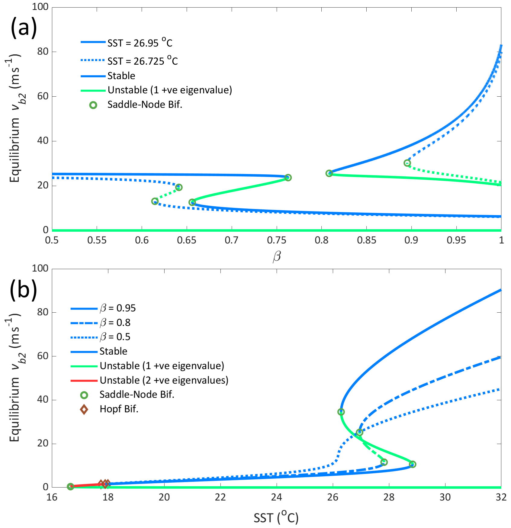
Figure 2 Bifurcation diagrams of model equilibria in (a) β and (b) SST. Blue denotes stable equilibria, green unstable (one positive eigenvalue), and red unstable (two positive eigenvalues). Saddle-node bifurcations are marked as circles, and Hopf bifurcations are marked as diamonds. In panel (a), for the dotted line, SST = 26.725 °C, and for the solid line, SST = 26.95 °C. In panel (b), for the dotted line, β=0.5; for the dashed line, β=0.8; and for the solid line, β=0.95.

The region of β–SST parameter space of interest for intensification or ERCs is the bistable region where both the low- and high-wind states exist. In this region and at its boundary, there is the possibility of transitioning between these states. These transitions could represent a few different phenomena. A transition from the low- to high-wind state can be interpreted as the intensification of a tropical depression into a TC and likewise, a transition from the high- to low-wind state as the dissipation of a TC into a tropical depression. A more nuanced phenomenon like an ERC consists of a cycle of multiple, and possibly incomplete, transitions between these stable states.

3.2 Rate-induced behaviour in the model

The effect of external forcing can be thought of as shifting the stability landscape while maintaining its qualitative features. If a tipping threshold, such as an unstable equilibrium, moves past the original position of a stable equilibrium of the unforced system, this stable equilibrium is said to be threshold-unstable to varying forcing rates (Wieczorek et al., 2023). When this threshold separates two stable equilibria, the system is said to be “basin-unstable”. Figure 3 shows a qualitative depiction of basin instability for the high-wind state in our model. In general, it has been shown that basin instability is a sufficient condition for rate-induced tipping to occur; that is, there exists some external forcing that will produce rate-induced tipping if the system is basin-unstable (Wieczorek et al., 2023). In many examples, it has been found that basin instability is both necessary and sufficient for rate-induced tipping to occur (Ritchie et al., 2023).

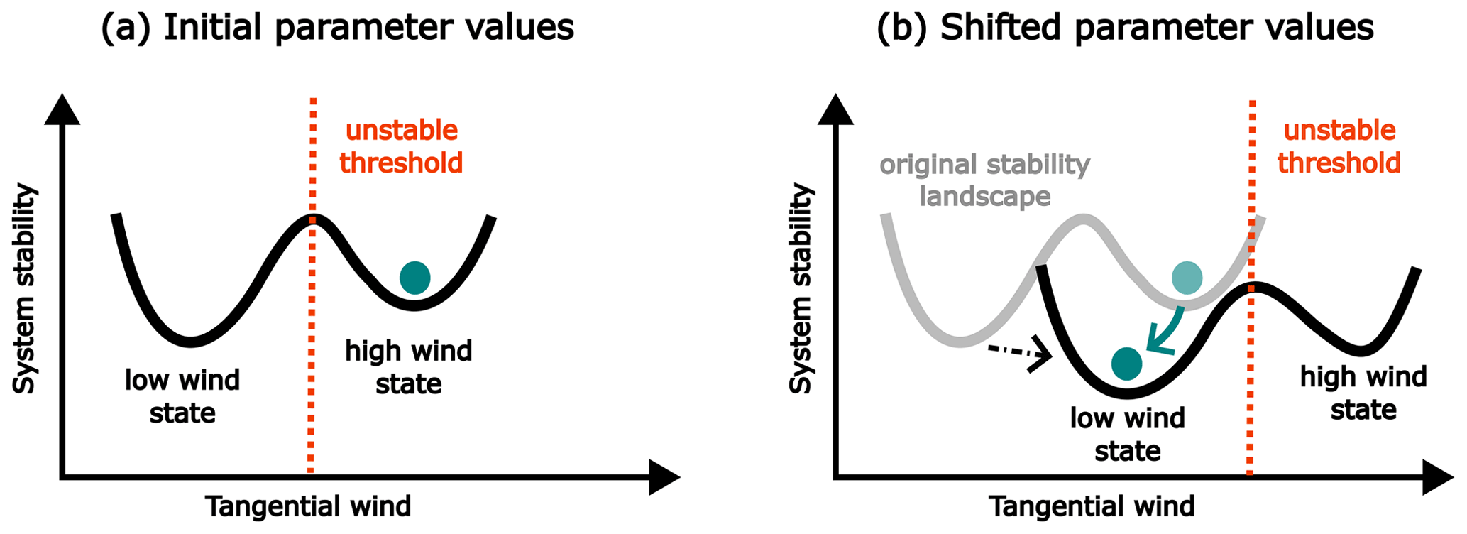
Figure 3 Schematic diagram for threshold instability or, in this case, basin instability. In panel (a), the stability landscape is shown for chosen initial values of the parameters. The two wells represent the two stable states of the model: low-wind and high-wind. The teal ball represents the system initialising from the high-wind state. The orange line represents the value of tangential wind at which there exists an unstable threshold. In panel (b), the stability landscape has shifted to a new location and shape due to a change in the parameter values. Note how the unstable threshold moves past the original location of the ball, thus causing it to roll into the well associated with the low-wind state. This schematic is adapted with permission from Ritchie et al. (2023, Fig. 1).

Here, we test for basin instability of the high-wind state in the β–SST phase space. We first choose a β–SST point and find the high-wind equilibrium that corresponds to this parameter choice. The system is then integrated forward in time over a range of fixed β and SST values while using the original equilibrium value as the initial condition. If for a given β–SST combination the system remains in the a high-wind state, this parameter pair is within the basin of attraction for that initial condition. Alternatively, if the system converges to a different equilibrium, which is the low-wind state here, then the parameter pair is not within the basin of attraction for that initial condition. Two examples of basin instability for the model are shown in Fig. 4. Here, we choose an initial condition for the high-wind state (the blue and red crosses) and test for tipping to the low-wind state. The red and blue curves are the basin instability boundaries that correspond to the respective initial condition. We see that the basin boundaries follow the saddle-node boundary for low and intermediate values of β, but for larger β the two diverge. This area of divergence is of interest as is shows where rate-induced tipping may occur (as opposed to traditional bifurcation-induced tipping across the saddle node).

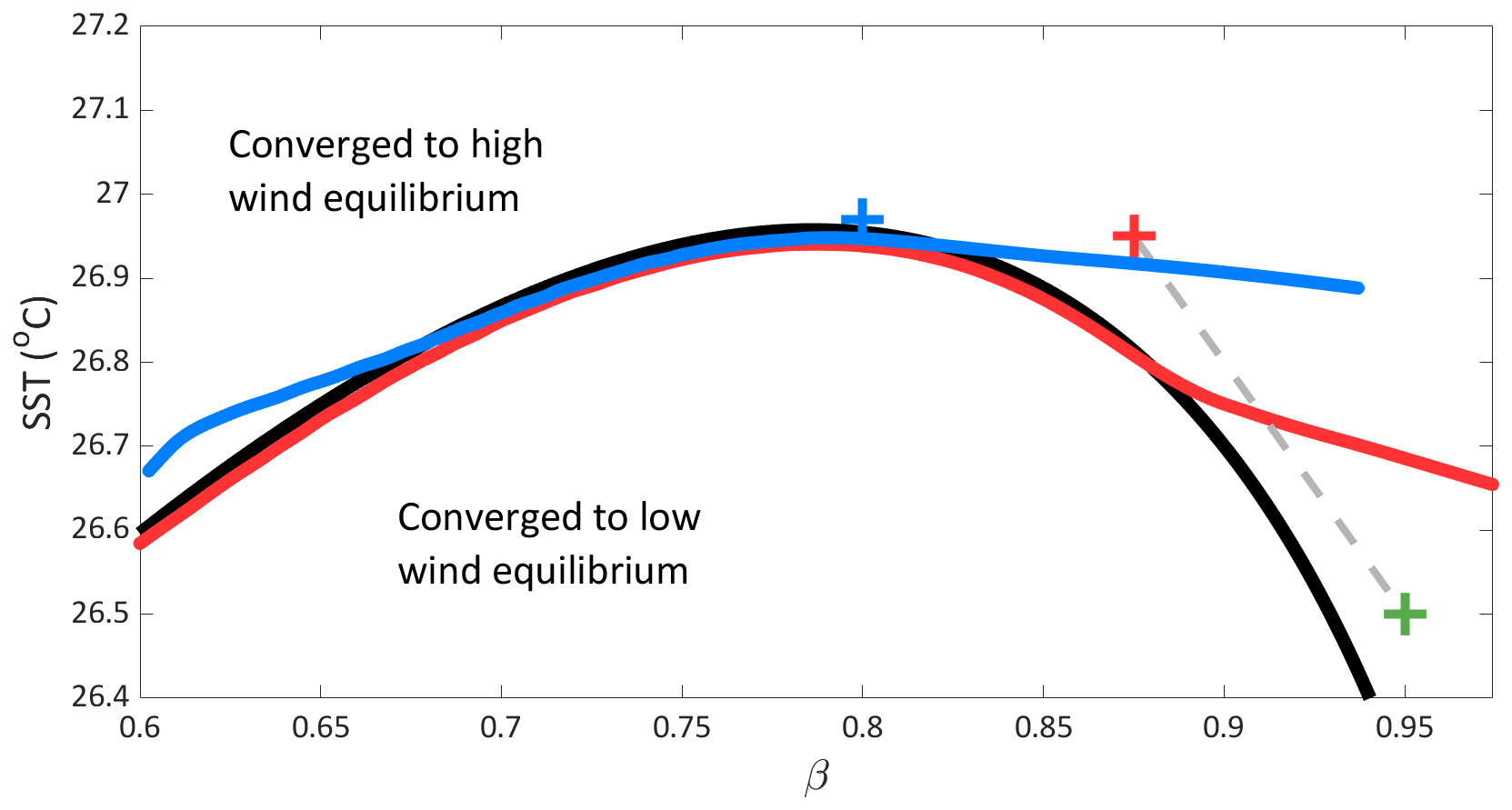
Figure 4 Examples of basin instability when considering instantaneous changes in β and SST. The initial conditions are denoted by the blue (β=0.8; SST = 26.97 °C) and red (β=0.875; SST = 26.95 °C) crosses, with their corresponding basin instability boundary in the same colour. The saddle-node continuation in β–SST, where the high-wind equilibrium begins, is given by the black line. The initial conditions converge to the high-wind equilibrium. Parameter conditions above the basin instability boundary lines re-converged to a high-wind equilibrium after the instantaneous change, and conditions below the line converged to a lower-wind equilibrium. The green cross (β=0.95; SST = 26.5) shows the conditions reached via forcing (profile trajectory shown in grey) in Fig. 5.

Using the information provided by the basin instability diagram shown in Fig. 4, we can produce examples of rate-induced tipping in the model. To define the evolution of a given parameter σ with time, we use a hyperbolic secant profile defined as

$$\begin{array}{}\text{(9)}& f(t;\mathit{\lambda },P)=\pm \text{sech}\left(\mathit{\lambda }\right(t-P\left)\right)+\mathrm{1},\end{array}$$

where the plus gives an increasing and the minus a decreasing profile, λ determines the rate of change, and P the time of peak forcing. This function was selected for its smooth transition between a defined maximum and minimum. Thus, for a given forcing parameter and maximum and minimum values (σ_minandσ_max) between which the forcing will occur, we define the time evolution of σ as

$$\begin{array}{}\text{(10)}& \mathit{\sigma }(t;\mathit{\lambda },P)={\mathit{\sigma }}_{\min }+({\mathit{\sigma }}_{\max }-{\mathit{\sigma }}_{\min })f(t;\mathit{\lambda },P).\end{array}$$

In cases where we require a strictly increasing or decreasing profile with no return to the original value, we define the evolution as

$$\begin{array}{}\text{(11)}& \mathit{\sigma }(t;\mathit{\lambda },P)=\left\{\begin{array}{ll}{\mathit{\sigma }}_{\min }+({\mathit{\sigma }}_{\max }-{\mathit{\sigma }}_{\min })f(t;\mathit{\lambda },P),& \text{if }t<P;\\ {\mathit{\sigma }}_{\min }\text{ or }{\mathit{\sigma }}_{\max },& \text{if }t>P.\end{array}\right.\end{array}$$

We consider a parameter path outlined by the dashed line in Fig. 4, with initial and final values given by the red and green crosses, respectively. Figure 5 shows a time integration of the system and the forcing profiles applied. The forcing profiles in the two examples differ only in their rates, which were chosen to be on either side of the critical rate. It is also important to note that the forcing profiles never reach the critical values which would push the system across a bifurcation point (as shown in Fig. 4). For the solid-line profile, with a rate λ of 0.1, we see the forcing is slow enough for the system to follow the high-wind state, leading to an intensification of the TC. For the dashed-line profile, with a rate λ of 0.3, the forcing exceeds the critical rate and the system crosses the unstable mid-wind-state threshold, causing it to tip to the low-wind state, leading to a dissipation of the TC.

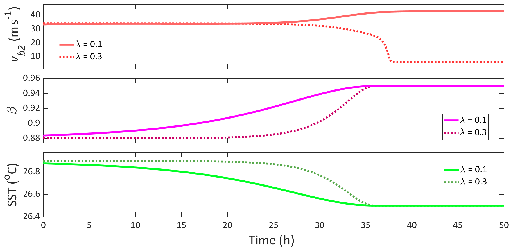
Figure 5 Example of the rate threshold between tracking and tipping when no bifurcation is crossed, with tangential wind speed and corresponding β and SST forcing profiles. For both the solid-line and dotted-line profiles, the maximum and minimum values of β and SST are the same (decreasing ramp profiles with $\mathrm{0.875}\le \mathit{\beta }\le \mathrm{0.95}$ and $\mathrm{26.5}\le \text{SST}\le \mathrm{26.95}$ °C). The solid forcing profiles have a rate of λ=0.1, and we see a tracking of the high-wind equilibrium, whereas the dotted forcing profiles have a rate of λ=0.3, and we see tipping to the low-wind equilibrium.

In Fig. 6, we provide some examples of overshoot recovery in the model. In Fig. 6a, β is forced with a return profile which crosses the saddle-node bifurcation. We see that a very small change in the forcing rate can determine whether the model recovers to the high-wind state or tips to the low-wind state. Interestingly, the system appears to move to the unstable mid-wind state for a considerable period of time before either recovering or tipping. The similarity between this behaviour and that observed in ERCs is discussed in Sect. 5. In Fig. 6b, similar behaviour can be seen for forcing of SST, where a small change to the rate at which a temporary reduction in SST occurs can determine whether the system recovers or tips. Here, however, instead of spending an intermediate period in the unstable mid-wind state, as with the β forcing, the system moves completely to the low-wind state before beginning to recover, the success of which is dependent on the forcing rate.

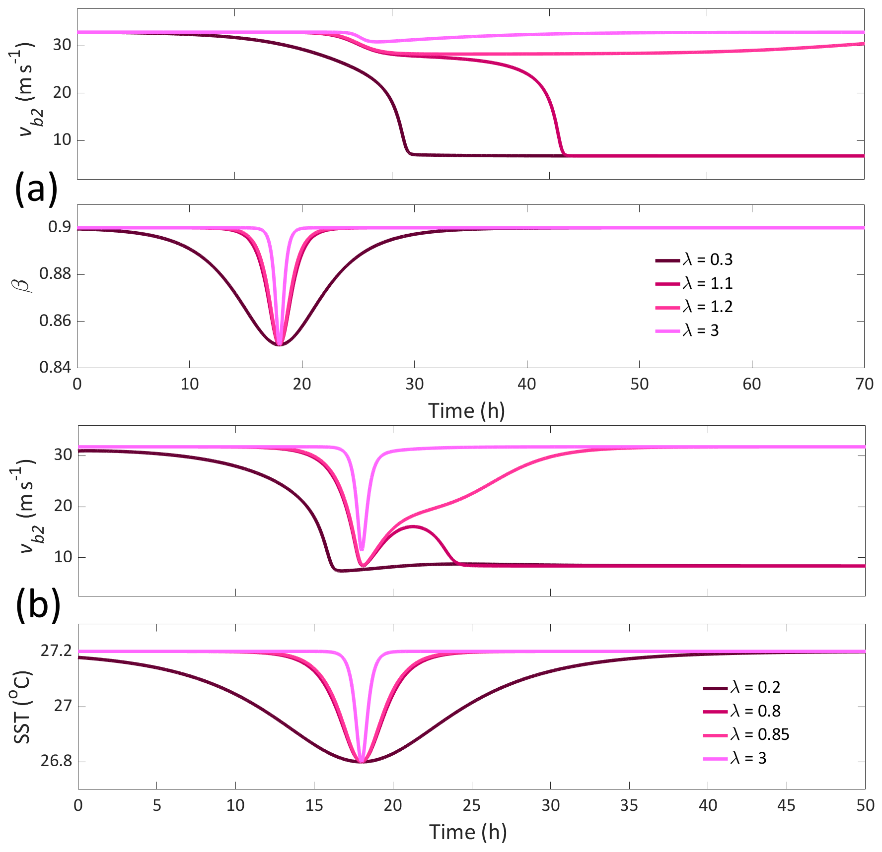
Figure 6 Example of the rate threshold between tipping and recovery when a bifurcation is crossed, with tangential wind speed and corresponding β or SST forcing profiles. In panel (a), β is forced between the same maximum and minimum (decreasing return profile with $\mathrm{0.85}\le \mathit{\beta }\le \mathrm{0.9}$), with fixed SST =26.725 °C for a range of forcing rates. In panel (b), SST is forced between the same maximum and minimum (decreasing return profile with $\mathrm{26.8}\le \text{SST}\le \mathrm{27.2}$ °C), with fixed β=0.8 for a range of forcing rates.

4 Case study: Hurricane Irma

Here, we test the ability of the low-order model to produce realistic tangential wind profiles, such as the one observed for Hurricane Irma (2017). Irma underwent two separate periods of rapid intensification (RI), the first shortly after its formation and a second as it moved into warmer waters around the edge of the Caribbean Sea (Fischer et al., 2020). In the context of this model, recreating the first RI period is of interest in relation to factors of TC intensification. The second is of interest in relation to the dynamics of ERCs.

The first period of RI lasted for approximately 2 d from its time of formation. This RI period saw the maximum tangential wind increase by 33 m s⁻¹ from approximately 18 to 51 m s⁻¹ (Fischer et al., 2020). During this time, Irma moved into an area of lower SST, meaning that a decreasing SST profile accompanies this RI period. In Fig. 7a are the results of the recreation of this intensification period. The SST profile was estimated using the best-track estimated latitude and longitude coordinates for Irma (Cangialosi et al., 2021) along with daily gridded SST data (NOAA, 2023). To initiate an intensification over this decreasing SST profile, we noted that the range over which SST is varying (27–28.5 °C) coincides with the range within which a saddle-node bifurcation occurs in the low-wind equilibrium (see Fig. 2b). We thus applied a decreasing return (hyperbolic secant) β forcing profile to tip the system over the low-wind-state bifurcation. Once the system crosses the bifurcation, it transitions to the high-wind equilibrium, producing an intensification of the TC. The β profile used in Fig. 7a has a λ of 0.15. We found that an increase in λ (e.g. λ=0.2) enabled the system to regain the low-wind equilibrium without tipping; that is, no intensification occurred. As the system still crosses the bifurcation point, this is an example of the overshoot recovery discussed in Sect. 3.2. Thus, in this context, we can describe the first RI as a “missed” return tipping.

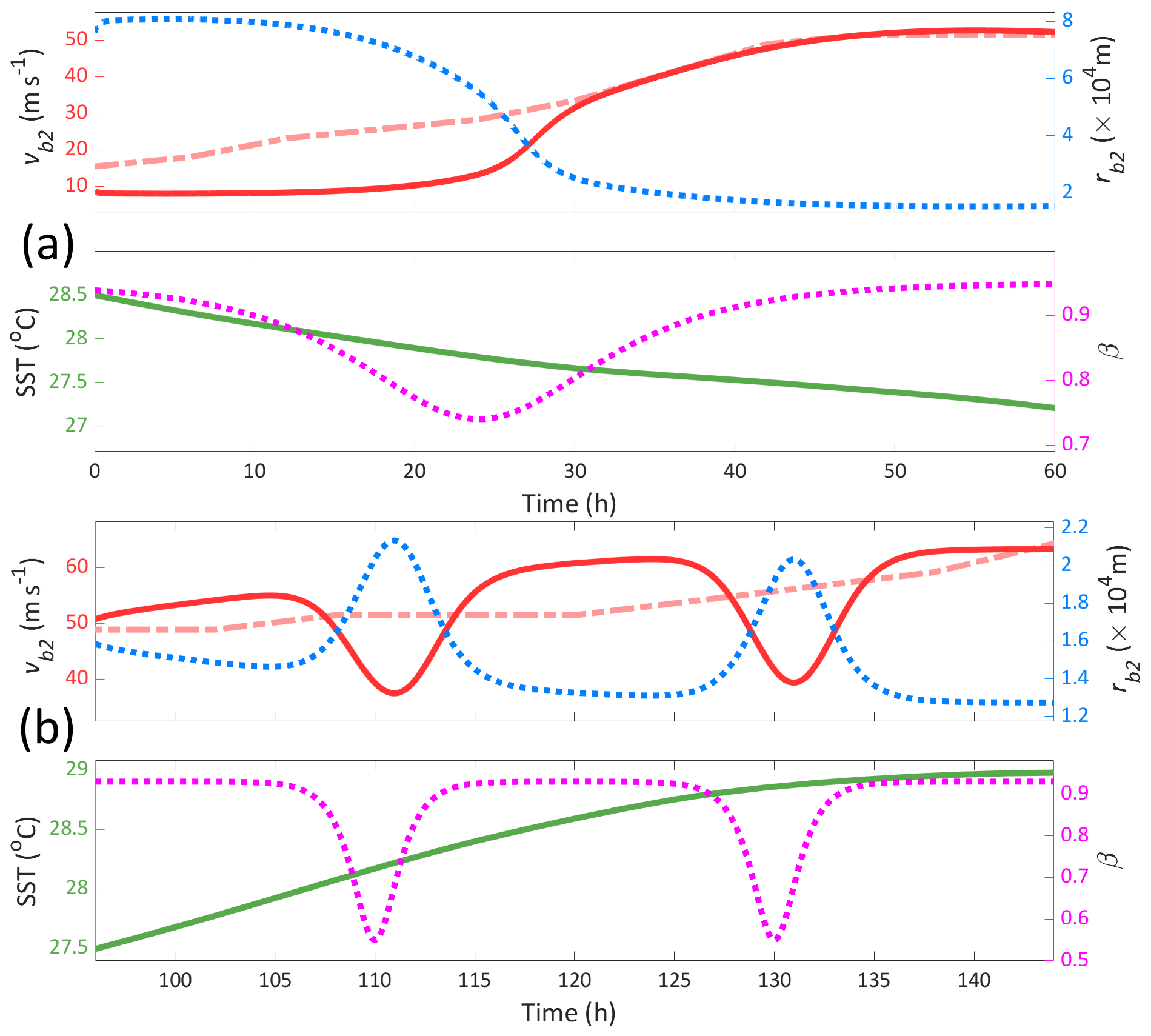
Figure 7 Comparison of tangential wind evolution between the model (solid red) and that observed for Hurricane Irma (dashed light-red). The model is forced with an SST profile estimated using Irma best-track data and daily gridded SST from NOAA (solid green) and a conceptual β profile (dotted pink). The outer eyewall boundary-layer radius (r_b2) is also shown (dotted blue). In panel (a), the first RI period is modelled with a decreasing return β profile ($\mathrm{0.74}\le \mathit{\beta }\le \mathrm{0.95}$, λ=0.15) so as to initiate tipping to the high-wind state. In panel (b), the second RI period is modelled with a double-decreasing β profile ($\mathrm{0.55}\le \mathit{\beta }\le \mathrm{0.93}$, λ=1) to recreate the two consecutive ERCs.

The second RI period began 5 d after its formation as it began to move over a region of increased SST. The RI period lasted 2 d and increased the maximum tangential wind speed to up to 80 m s⁻¹. The second RI period was characterised by two consecutive ERCs. The ERCs observed in Irma occurred over a much shorter time span than is typical of ERCs, each taking around 10 h versus the average of 36 h (Sitkowski et al., 2011; Fischer et al., 2020). Although the wind profiles of the secondary eyewalls and the ERC event were not directly measured, Fischer et al. (2020) estimated a radial wind profile of the event using NOAA fly-through data. To recreate a similar scenario, we forced the model with the estimated SST profile for the second RI period and a double-decreasing return β profile. This resulted in an overall increase in tangential wind, with two isolated reductions corresponding to the change in β. When interpreting changes in the eyewall radius (r_b2) to track the radius of maximum wind (RMW), the model produces a change in the RMW during the ERC events on a similar scale to that estimated by Fischer et al. (2020) (magnitude of ×10⁴ m).

5 Discussion

The observed tipping in this low-order model is between two stable states, both of which represent a storm with primary circulation. This is a distinctive feature of the model, noting that other low-order dynamical models for TCs have tipping between an “on” and an “off” state (see e.g. Slyman et al., 2024). A natural question is then whether or not multiple stable states of varying cyclone intensity exist in models of higher complexity. The nonhydrostatic Cloud Model 1 (CM1; Bryan and Fritsch, 2002) has been widely used to model the internal dynamics throughout the lifespan of a tropical cyclone. In a study on formation timescales under increasing SST, Ramsay et al. (2020) used CM1 to simulate an ensemble of TCs for each SST where initial conditions are randomised through small-amplitude potential temperature perturbations. The temporal behaviour of maximum azimuthal-mean tangential wind at 25 m is shown (Fig. 2 in Ramsay et al., 2020). It can be seen that individual storms after maturation experience periods of a reduction in the maximum wind before regaining previous strength. This is indicative of the existence of multiple stable states, i.e. a low- and high-wind state. Such transitioning behaviour is more pronounced as SST increases. These results suggest the existence of the stable low-wind state in a more complex TC model, and thus our findings could inform further studies of tipping behaviour for more realistic simulations.

It is informative to highlight the justification for the β forcing profiles used in Sect. 3. We discussed the theories of Kepert (2013) and Ge et al. (2015) regarding the role of the vorticity gradient in ERCs and intensification, outlined the inclusion of vorticity in the model, and described the connection between β and the vorticity gradient via the tangential wind profile and radial inflow. Thus, interpreting a dip in β as representing a change in the radial vorticity gradient follows directly from Eq. (8). We see that a decrease in β increases the radial vorticity gradient on the outer eyewall boundary. This change is in line with both Kepert (2013) and Ge et al. (2015), where an increase in the radial vorticity gradient is responsible for an ERC or intensification. As box models, such as this one, are not defined over a spatial domain, it is necessary to interpret changes in the radial vorticity gradient throughout the boundary layer as changes at the outer eyewall boundary. We acknowledge that this does not allow for the definition of multiple radial vorticity gradient maxima as used by Kepert (2013) or the definition of differing inner-core vorticity profiles as used by Ge et al. (2015). Instead, this study has shown that at the level of a low-order conceptual model, a temporary increase in the radial vorticity gradient can initiate intensification (Fig. 7a) and dissipation (Figs. 5 and 6), with some examples suggesting ERC-like behaviour (Fig. 7b).

The β and SST forcing profiles used in this study can be likened to various physical situations. Return profiles, such as in Fig. 6, model a temporary reduction and return of the parameter value. In the case of β, such a profile would be caused by a temporary restriction to the radial inflow of the TC. One interesting scenario where such variation in the radial inflow has been observed is in the diurnal variation in TC boundary-layer flow (Zhang et al., 2020). These daily changes in the boundary layer produce return profiles in the radial inflow of similar shape and over similar time spans to those used in Fig. 6. In the case of SST, return profiles represent the movement of the TC over an isolated area of cooler or warmer (for an increasing return profile) SST. For example, the forcing profiles like the one used in Fig. 6 could model a physical situation such as the movement of a TC over a region of upwelling of cooler water from the deep ocean as has been observed within TC regions (Park and Kim, 2010). The interaction of TCs with SST temperature profiles such as these has been observed to produce interesting behaviour, such as in the case of Tropical Cyclone Nari (2001), which moved back and forth across the Kuroshio Current multiple times, causing its intensity to fluctuate. The rapid change in SST experienced by Nari as it oscillated across the warmer water of the Kuroshio and the cooler surrounding sea could have produced SST profiles similar to those used here. In comparison to return profiles, ramp profiles, such as in Fig. 5, model gradual and continuing increases or decreases in the parameter values. These ramp profiles are useful for recreating the conditions often present during TC intensification as seen in Fig. 7, where the estimated SST for Hurricane Irma produced a similarly shaped profile.

The discovery of rate-induced tipping in the low-order TC model suggests that external forcing rates play a role in TC dynamics. Very little research has been conducted into rate-induced phenomena in TCs. In a recent analysis of a low-order model representing TC formation, Slyman et al. (2024) identified rate-induced tipping by forcing two different parameters: potential velocity and wind shear. These findings point to the possibility of rate-induced tipping pervading multiple aspects of TC dynamics.

We also found that the rate of forcing determines the system's ability to overshoot a bifurcation point but recover its original equilibrium. No previous research has been done on the temporary exceeding of critical parameter levels in TC models. In the case of this TC model, these brief parameter anomalies can have nice interpretations in terms of the movement of a TC through changing environmental conditions.

Observations of rate-dependent phenomena as described here have direct implications for TC prediction. Quantities such as a TC's tracking speed and the SST distribution in its path can be measured, thus allowing for approximations of rates of external forcing. Due to the conceptual nature of the model, we have focused on the qualitative behaviour that can result from different forcing rates. In order to make quantitative predictions about critical rates of forcing, further research of rate-induced tipping in higher complexity spatially extended TC models coupled with more realistic forcing profiles will be needed.

The results of this study broaden our understanding of the role of the vorticity gradient as a driver of TC behaviour. They also expand upon the general dynamical properties of TCs. From these results, it is clear there are potential advances to be made in TC modelling and prediction by further research in this area.

Appendix A: Supplementary model outline

A1 Auxiliary equations

A detailed derivation of these governing equations is provided by S&F (Schönemann and Frisius, 2012). Only an overview of the important components is presented here.

A1.1 Mass-stream function

The Boussinesq approximation ensures non-divergence of the radial and vertical flow within the boundary layer, and hence a mass-stream function for the boundary layer may be introduced as

$$\begin{array}{}\text{(A1)}& {\mathrm{\Psi }}_{\mathrm{b}}=\mathrm{2}\mathit{\pi }{r}_{\mathrm{b}}{\mathit{\rho }}_{\mathrm{b}}{C}_D{\displaystyle \frac{\left|v_{\mathrm{b}}\right|v_{\mathrm{b}}}{{\mathit{\zeta }}_{\mathrm{b}}}},\end{array}$$

where the subscript b denotes evaluation at z=H_b, C_D is the transfer coefficient for momentum, and ζ is the absolute vorticity. For the purposes of this model, the mass-stream function is only considered at the outer edge of the eyewall boundary layer, i.e. Ψ_b2.

A1.2 Physical radius and tangential velocity

The model applies a version of the thermal wind balance equation derived by Emanuel (1986). Assuming gradient wind balance, saturated pseudoadiabatic ascent, and conservation of angular momentum, Emanuel takes the radial thermal wind balance and assumes the specific volume ($\mathrm{1}/\mathit{\rho }$) to be expressible as a function of pressure and saturated entropy. Coupled with the assumption that the saturated entropy does not vary along surfaces of equal angular momentum, this allows the thermal wind balance to be expressed as a relationship between (specific) saturated entropy, s^*, and the angular momentum per unit mass, m:

$$\begin{array}{}\text{(A2)}& {\displaystyle \frac{T_{\mathrm{b}}-T}{m}}{\displaystyle \frac{\mathrm{d}{s}^{*}}{\mathrm{d}m}}=\mathrm{2}{\displaystyle \frac{T_{\mathrm{b}}-T}{f^{\mathrm{2}}{R}^{\mathrm{3}}}}{\displaystyle \frac{\mathrm{d}{s}^{*}}{\mathrm{d}R}}={\displaystyle \frac{\mathrm{1}}{r^{\mathrm{2}}}}-{\displaystyle \frac{\mathrm{1}}{r_{\mathrm{b}}^{\mathrm{2}}}},\end{array}$$

where T denotes temperature, $r\equiv r(z;R)$ is the physical radius of a given potential radius, and r_b≡r_b(R) is the physical radius in the boundary layer corresponding to the potential radius. This balance relates the angular momentum surfaces to the potential radius and the change in saturated entropy with potential radius. Thus, equations for the evolution of the physical radii of the inner and outer edges of the eyewall boundary layer are found by taking R=R₁ and R=R₂ and approximating the change in saturated entropy (via finite difference). For closure the mass, M, enclosed by the angular momentum surface at R=R₂ is assumed to be conserved, and as the eye is modelled by solid body rotation, its mass, M_e, enclosed by the angular momentum surface at R=R₁, will also be conserved. Using the Boussinesq approximation of near-constant density, these masses can be found (derived by Frisius, 2005) by

$$\begin{array}{}\text{(A3a)}& M=\mathit{\pi }\mathit{\rho }\underset{H_{\mathrm{b}}}{\overset{H+H_{\mathrm{b}}}{\int }}{r}_{\mathrm{2}}^{\mathrm{2}}\mathrm{d}z={\displaystyle \frac{\mathit{\pi }\mathit{\rho }}{G_{\mathrm{2}}}}\ln \left(\mathrm{1}+G_{\mathrm{2}}{r}_{\mathrm{b}\mathrm{2}}^{\mathrm{2}}H\right)\end{array}$$

and

$$\begin{array}{}\text{(A3b)}& M_{\mathrm{e}}=\mathit{\pi }\mathit{\rho }\underset{H_{\mathrm{b}}}{\overset{H+H_{\mathrm{b}}}{\int }}{r}_{\mathrm{1}}^{\mathrm{2}}\mathrm{d}z={\displaystyle \frac{\mathit{\pi }\mathit{\rho }}{G_{\mathrm{1}}}}\ln \left(\mathrm{1}+G_{\mathrm{1}}{r}_{\mathrm{b}\mathrm{1}}^{\mathrm{2}}H\right),\end{array}$$

where r₁ and r₂ are the physical radii of the angular momentum surfaces at R=R₁ and R=R₂, respectively, and r_b1 and r_b2 are the physical radii of the inner (R=R₁) and outer (R=R₂) edges of the eyewall boundary layer. The functions G₁ and G₂ are given as

$$\begin{array}{}\text{(A4)}& \begin{array}{rl}{G}_{\mathrm{2}}\left(s_{\mathrm{i}}^{*}\right)& ={\displaystyle \frac{\mathrm{2}\mathrm{\Gamma }}{f^{\mathrm{2}}{R}_{\mathrm{2}}^{\mathrm{3}}}}{\displaystyle \frac{s_{\mathrm{a}}^{*}-s_{\mathrm{i}}^{*}}{\mathrm{\Delta }R}},\\ G_{\mathrm{1}}\left(s_{\mathrm{i}}^{*}\right)& ={\displaystyle \frac{\mathrm{2}\mathrm{\Gamma }}{f^{\mathrm{2}}{R}_{\mathrm{1}}^{\mathrm{3}}}}{\displaystyle \frac{s_{\mathrm{a}}^{*}-s_{\mathrm{i}}^{*}}{\mathrm{\Delta }R}}{\left({\displaystyle \frac{R_{\mathrm{1}}}{R_{\mathrm{2}}}}\right)}^{\mathit{\kappa }-\mathrm{1}},\end{array}\end{array}$$

where Γ is the temperature lapse rate, f is the Coriolis parameter, and κ is called the eyewall entropy profile parameter and controls the radial decrease in saturated entropy away from the radius of maximum wind at R₂. The temperature lapse rate controls the vertical temperature profile, which, in this model, is taken to be linear and defined as

$$\begin{array}{}\text{(A5)}& \mathrm{\Gamma }={\displaystyle \frac{T_{\mathrm{s}}-T_t}{H}},\end{array}$$

where T_t is the tropopause temperature, T_s is the sea-surface temperature, and H is the tropopause height. The mass equations (A3a) can then be rearranged to find r_b1 and r_b2 as

$$\begin{array}{}\text{(A6)}& \begin{array}{rl}{r}_{\mathrm{b}\mathrm{2}}\left(s_{\mathrm{i}}^{*}\right)& =\sqrt{{\displaystyle \frac{\mathrm{1}}{G_{\mathrm{2}}H}}\left[\exp \left({\displaystyle \frac{G_{\mathrm{2}}M}{\mathit{\pi }\mathit{\rho }}}\right)-\mathrm{1}\right]},\\ r_{\mathrm{b}\mathrm{1}}\left(s_{\mathrm{i}}^{*}\right)& =\sqrt{{\displaystyle \frac{\mathrm{1}}{G_{\mathrm{1}}H}}\left[\exp \left({\displaystyle \frac{G_{\mathrm{1}}{M}_{\mathrm{e}}}{\mathit{\pi }\mathit{\rho }}}\right)-\mathrm{1}\right]},\end{array}\end{array}$$

and using Eq. (2), the corresponding tangential wind speeds at these points can be found by

$$\begin{array}{}\text{(A7)}& \begin{array}{rl}{v}_{\mathrm{b}\mathrm{2}}\left(s_{\mathrm{i}}^{*}\right)& ={\displaystyle \frac{f}{\mathrm{2}}}\left({\displaystyle \frac{R_{\mathrm{2}}^{\mathrm{2}}-r_{\mathrm{b}\mathrm{2}}^{\mathrm{2}}}{r_{\mathrm{b}\mathrm{2}}}}\right),\\ v_{\mathrm{b}\mathrm{1}}\left(s_{\mathrm{i}}^{*}\right)& ={\displaystyle \frac{f}{\mathrm{2}}}\left({\displaystyle \frac{R_{\mathrm{1}}^{\mathrm{2}}-r_{\mathrm{b}\mathrm{1}}^{\mathrm{2}}}{r_{\mathrm{b}\mathrm{1}}}}\right).\end{array}\end{array}$$

A1.3 Mass

As the eye and eyewall mass (M_e, M_i, $M=M_{\mathrm{e}}+M_{\mathrm{i}}$) are assumed to be conserved, they can be calculated for the resting state when the eyewall boundaries are assumed to be vertically oriented, i.e. r₁=R₁ and r₂=R₂. They are then

$$\begin{array}{}\text{(A8)}& \begin{array}{rl}{M}_{\mathrm{e}}& =\mathit{\pi }\mathit{\rho }H{R}_{\mathrm{1}}^{\mathrm{2}},M=\mathit{\pi }\mathit{\rho }H{R}_{\mathrm{2}}^{\mathrm{2}},\\ M_{\mathrm{i}}& =M-M_{\mathrm{e}}=\mathit{\pi }\mathit{\rho }H\left(R_{\mathrm{2}}^{\mathrm{2}}-R_{\mathrm{1}}^{\mathrm{2}}\right).\end{array}\end{array}$$

The masses of the boundary layer beneath the eyewall (M_bi) and the ambient region (M_ba) are not assumed to be conserved and are given by

$$\begin{array}{}\text{(A9)}& \begin{array}{rl}{M}_{\mathrm{bi}}\left(s_{\mathrm{i}}^{*}\right)& =\mathit{\pi }{\mathit{\rho }}_{\mathrm{b}}{H}_{\mathrm{b}}\left(r_{\mathrm{b}\mathrm{2}}^{\mathrm{2}}-r_{\mathrm{b}\mathrm{1}}^{\mathrm{2}}\right),\\ M_{\mathrm{ba}}\left(s_{\mathrm{i}}^{*}\right)& =\mathit{\pi }{\mathit{\rho }}_{\mathrm{b}}{H}_{\mathrm{b}}\left(r_{\mathrm{ba}}^{\mathrm{2}}-r_{\mathrm{b}\mathrm{2}}^{\mathrm{2}}\right),\end{array}\end{array}$$

where r_ba is the outer radius of the ambient region.

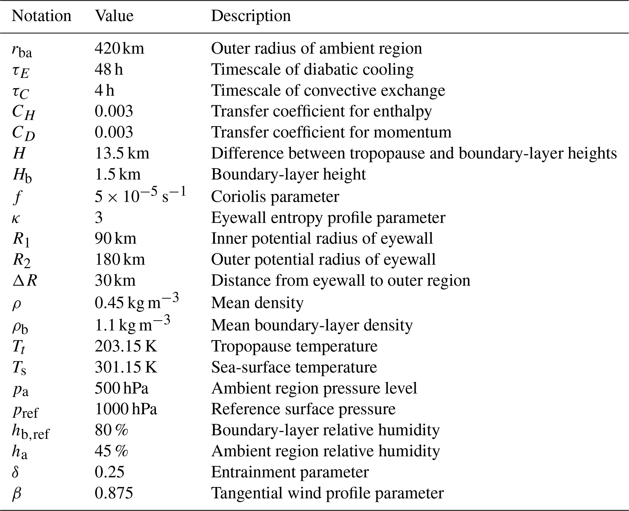
Table A1 Model parameters given by S&F (Schönemann and Frisius, 2012).

A1.4 Entropy

The entropy of the sea surface underneath the eyewall region is taken to be

$$\begin{array}{}\text{(A10)}& \begin{array}{rl}{s}_{\mathrm{oi}}\left(s_{\mathrm{i}}^{*}\right)& =L_v\left({\displaystyle \frac{q_v^{*}-q_{\mathrm{v},\mathrm{ref}}}{T_{\mathrm{s}}}}\right)+{\displaystyle \frac{v_{\mathrm{b}\mathrm{2}}^{\mathrm{2}}}{\mathrm{2}{T}_{\mathrm{s}}\mathit{\beta }}}\left[\mathrm{1}-{\left({\displaystyle \frac{r_{\mathrm{b}\mathrm{2}}}{r_{\mathrm{a}}}}\right)}^{\mathrm{2}\mathit{\beta }}\right]\\ & -{\displaystyle \frac{f{v}_{\mathrm{b}\mathrm{2}}{r}_{\mathrm{b}\mathrm{2}}}{T_{\mathrm{s}}\left(\mathrm{1}-\mathit{\beta }\right)}}\left[\mathrm{1}-{\left({\displaystyle \frac{r_{\mathrm{a}}}{r_{\mathrm{b}\mathrm{2}}}}\right)}^{\mathrm{1}-\mathit{\beta }}\right],\end{array}\end{array}$$

where L_v is the latent heat of vaporisation, $q_v^{*}$ is the specific humidity at saturation, and q_v,ref is the reference specific humidity. The entropy of the sea surface far from the TC (R→∞) is taken to be

$$\begin{array}{}\text{(A11)}& s_{\mathrm{oa}\mathrm{0}}=L_v\left({\displaystyle \frac{q_v^{*}-q_{\mathrm{v},\mathrm{ref}}}{T_{\mathrm{s}}}}\right),\end{array}$$

and the sea-surface entropy under the ambient region is taken to be the average of these two:

$$\begin{array}{}\text{(A12)}& s_{\mathrm{oa}}\left(s_{\mathrm{i}}^{*}\right)={\displaystyle \frac{s_{\mathrm{oi}}+s_{\mathrm{oa}\mathrm{0}}}{\mathrm{2}}}.\end{array}$$

The entropy of the ambient region itself is taken to be

$$\begin{array}{}\text{(A13)}& s_{\mathrm{a}}=L_v\left({\displaystyle \frac{q_{v,\mathrm{a}}}{T_{\mathrm{a}}}}-{\displaystyle \frac{q_{\mathrm{v},\mathrm{ref}}}{T_{\mathrm{ref}}}}\right)-R_{\mathrm{d}}\ln \left({\displaystyle \frac{p_{\mathrm{a}}}{p_{\mathrm{ref}}}}\right)+c_p\ln \left({\displaystyle \frac{T_{\mathrm{a}}}{T_{\mathrm{ref}}}}\right),\end{array}$$

where q_v,a is the specific humidity of the ambient region, T_ref is a reference temperature, R_d is the specific gas constant of dry air, p_a is the pressure of the ambient region, p_ref is a reference pressure, c_p is the specific heat of dry air at constant pressure, and T_a is the temperature of the ambient region defined as

$$\begin{array}{}\text{(A14)}& T_{\mathrm{a}}=T_{\mathrm{s}}{\left({\displaystyle \frac{p_{\mathrm{a}}}{p_{\mathrm{ref}}}}\right)}^{\frac{R_{\mathrm{d}}\mathrm{\Gamma }}{g}}.\end{array}$$

For the saturated entropy of the ambient region, $s_{\mathrm{a}}^{*}$, the specific humidity is taken at saturation ($q_{v,\mathrm{a}}^{*}$ instead of q_v,a).

A2 Constant parameter values

The model parameters used by S&F are given in Table A1.

A3 Specific humidity

S&F do not provide values for the specific humidities $q_v^{*},q_{v,\mathrm{a}},q_{v,\mathrm{a}}^{*}$, and q_v,ref. To calculate the specific humidity at saturation from the air temperature, we fit a two-term exponential model to experimental data (ToolBox, 2009) (exp2 function in MATLAB), which resulted in

$$\begin{array}{}\text{(A15)}& q^{*}\left(T\right)=\mathrm{1.445}\times {\mathrm{10}}^{-\mathrm{6}}{e}^{\mathrm{0.221}T}+\mathrm{4.967}{e}^{\mathrm{5.718}\times {\mathrm{10}}^{-\mathrm{2}}T},\end{array}$$

where T is the temperature in degrees Celsius. Then, $q_v^{*}$ is calculated at T_s and $q_{v,\mathrm{a}}^{*}$ at T_a. The non-saturated humidities are then calculated as $q_{\mathrm{v},\mathrm{ref}}=h_{\mathrm{b},\mathrm{ref}}{q}_v^{*}$ and $q_{v,\mathrm{a}}=h_{\mathrm{a}}{q}_{v,\mathrm{a}}^{*}$. When comparing the function output with observational data of specific humidity gathered during TC season (Jordan, 1958), values for q_v,ref were close to those observed, but the values of q_v,a were smaller than observed; thus, we scaled $q_{v,\mathrm{a}}^{*}$ by a factor of 1.7 to match with observations. We assume this discrepancy is a result of Eq. (A15), which only considers the temperature difference and not the pressure difference between the two regions. We also take the reference temperature, T_ref, to be equal to the sea-surface temperature, T_s.