the Creative Commons Attribution 4.0 License.
the Creative Commons Attribution 4.0 License.
 | 13 Aug 2024
Prognostic assumed-probability-density-function (distribution density function) approach: further generalization and demonstrations
Jun-Ichi Yano
A methodology for directly predicting the time evolution of the assumed parameters for distribution densities based on the Liouville equation, as proposed earlier, is extended to multidimensional cases and to cases in which the systems are constrained by integrals over a part of the variable range. The general formulation developed here is applicable to a wide range of problems, including the frequency distributions of subgrid-scale variables, hydrometeor size distributions, and probability distributions characterizing data uncertainties. The extended methodology is tested against a convective energy-cycle system and the Lorenz strange attractor. As a general tendency, the variance tends to collapse to a vanishing value over a finite time, regardless of the chosen assumed distribution form. This general tendency is likely due to a common cause, as the collapse of the variance is commonly found in ensemble-based data assimilation due to low dimensionality.
- Article
(7131 KB) - Full-text XML
- BibTeX
- EndNote


A noble manner to characterize nonlinear systems is by predicting the evolution of the distributions of variables in space as well as the frequency distributions of variables at a single macroscopic point and as probabilities. Important applications in geophysics include subgrid-scale parameterizations based on the distribution density functions (DDFs: Sommeria and Deadorff, 1977; Mellor, 1977; Bougeault, 1981; LeTreut and Li, 1991; Bechtold et al., 1992, 1995; Richard and Royer, 1993; Bony and Emanuel, 2001; Golaz et al., 2002; Tompkins, 2002), the particle-size distributions in cloud microphysics (cf. Khain et al., 2015; Khain and Pinsky, 2018), and the characterizations of data and model uncertainties by the probability density functions (PDFs) in data assimilations (Carrassi et al., 2018; Evensen et al., 2022). Readers are referred to Yano et al. (2018) for backgrounds of the present study in the numerical weather forecast. Yano et al. (2024), hereafter referred to as YLP, proposed a general methodology for evaluating the evolution of these distributions in an efficient manner. The essence of their approach may be called “prognostic assumed-PDF (DDF)”, as an extension of the classical assumed-PDF approaches (cf. Golaz et al., 2002).
The present study constitutes a sequel to the YLP study. Here, the uniqueness of this work lies in carrying out a very solid analysis of the performance by directly comparing the assumed-PDF results with direct numerical results from the Liouville equation using some simple dynamical systems. A basic, but general, robust formulation provided by YLP enables this kind of comparison: this is not possible with the current existing assumed-PDF schemes, as reviewed in the introduction of YLP, because these are formulated only in a case-by-case manner with specific applications in mind. Thus, the performance of those schemes cannot be tested by simple dynamical systems. The robustness of the proposed formulation is discussed extensively in YLP.
The goal of the present paper is to test this formulation using more advanced cases. In YLP, only one-variable cases under relatively simple constraints (i.e., output conditions) were considered. The purpose of the present work is to (1) further generalize this methodology to multidimensional systems with more general constraints and (2) present further demonstrative cases. The present study is considered one of the first steps in making this new novel approach for computing distributions prognostically into operations. Some difficulties encountered are also discussed with respect to this ultimate goal.
The presentation of this work will be developed in the following manner: Sect. 2 briefly summarizes the formulation presented in YLP, whose details and extensive references are to be consulted in the original paper, and generalizes it to cases in which (1) constraints are defined over limited integral ranges and (2) different assumed distribution forms are assumed over the different domains; Sect. 2 generalizes one-variable results for the assumed-PDF formulation into the multivariable systems in a general manner, without specifying a PDF form; and Sect. 3 shows (in a more concrete manner) how these general formulations can be used when a Gaussian distribution with two variables is assumed. This example also suggests how reductions with different assumed-PDF forms can be proceeded. The general formulations presented in Sects. 2 and 3 are applied to the two dynamical systems in Sects. 4 and 5: (i) the two-variable convective energy-cycle system introduced by Yano and Plant (2012) (Sect. 4) and (ii) the three-variable system of the Lorenz strange attractor (Sect. 5). Three different assumed-PDF forms are considered for each system, and the results are discussed. Section 6 summarizes the results and presents further discussions.
2.1 Basic formulation
The basic formulation presented in YLP is summarized first; however, the reader is referred to the original paper for details. Let us assume a dynamical system with a single variable, ϕ, and that a distribution of ϕ can be approximately represented by an assumed form
which is characterized by N parameters, λj (). We also separately introduce a normalization factor, λ0, that satisfies a relation of p∝λ0. It follows that
The distribution Eq. (1) is normalized by
Here and in the following, an unspecified integral range may be taken from −∞ to +∞ for many of the physical variables, but some physical variables are semi-positive definite (e.g., temperature and mixing ratios). In the latter case, the integral range above must be from 0 to +∞.
The evolution of this distribution, p, is governed by the Liouville equation,
when the dynamical system is defined by . From the time derivative of Eq. (3),
By inserting Eq. (1) into Eq. (4), weighting it by σl (), and integrating it over the full variable range, we obtain a final expression for the prognostic equation for the distribution parameters, {λj}:
for . We can see from Eq. (6) that the weights, σl, are most conveniently chosen in such a manner that
constitute the constraints for this distribution: YLP suggest choosing these constraints (Eq. 7) to be the outputs that are required in a host model, and they call it the “output-controlled distribution principle”. As the left-hand side is equal to , Eq. (6) can predict these constraints in a self-consistent manner under an assumed form of Eq. (1). The core part of the derivation of this formulation and further discussion on the meaning of the weight σl are presented fully in Sect. 5.1 of YLP.
In the following two subsections, this basic formulation is generalized into two cases: first, constraints are defined over limited integral ranges of the distribution variable, ϕ; second, as a consequence, distributions take different forms over those limited ranges. This generalization is important in many operational applications; for example, in cloud schemes, various conditional statistics, including the cloud fraction, must be evaluated by restricting the integrals above saturation in the total-water distribution.
2.2 When the constraints are defined over limited integral ranges
Here, we generalize the above basic formulation to cases in which the different constraints are introduced over two different ranges of the distribution variables. More specifically, we assume that the distribution variable, ϕ, is defined over , and the constraints are introduced in analogy with Eq. (6), although differently over the two ranges, and :
as a generalization of Eq. (7). In the above expressions, by following the output-constrained distribution principle proposed in YLP. Here, in the following abstract examples, there is no host model looking for outputs from a system defining a distribution. Thus, we will simply set those constraints to be the means and variances, as well as covariances, of the system, with priority given to defining the former under a given number of PDF parameters.
In this case, the variational principle to maximize the information entropy with the given constraints (cf. Sect. 3.1.1 of YLP) is given by the following:
It then reduces to the following:
Thus, the most likely distribution under the constraints (Eq. 8a, b) is
Note that , due to the continuity of p, when at ϕ=0.
2.3 When the distribution takes different forms in two different domains
In the last subsection, the constraints have been generalized to a case in which they are defined over two limited ranges of the distribution variable, ϕ; see Eq. (8a) and (8b). As it turns out, the most likely distribution (Eq. 10) under these constraints also takes different forms over these two ranges. Consequently, the formulation for predicting the given PDF parameters must also be generalized to such cases: this subsection addresses this issue.
By following the last subsection, we divide the variable range into the two subdomains and and assume that the distribution takes different forms over those two subdomains. Thus,
assuming for now. By continuity, at ϕ=0, . Again, we assume that the first parameters, , are the normalization factors; thus,
Especially when , as is the case with the result from Eq. (10), it follows that . Here, the assumed form of Eq. (11) follows from the constraints of the form in Eq. (8a) and (8b).
By applying the time derivative to the normalization condition,
we find
which reduces to
Here, and , where
After substituting the assumed-PDF form in Eq. (11) and applying the chain rules on the time derivative in the Liouville equation (i.e., Eq. 4), it reduces to the following:
By applying weighted integrals on both and then further substituting Eq. (14) into the above, we obtain a pair of equations for predicting the PDF parameters:
for .
2.4 Multidimensional case (I)
The formulations introduced in the last subsections are now further generalized into a multidimensional case, in which the distribution depends on more than one variable. This variable set is treated as a vector, x, with the first component corresponding to x. Here, note a change in the notation for the distribution variable from ϕ to x in the following.
As in the last two subsections, we assume that a given system is constrained differently depending on the sign of x. More precisely, we assume that there are N constraints that are defined differently for the different sign of x as well as M additional constraints that are defined to be independent of the sign of x. Consequently, the weights to be introduced are as follows: , for , and , for , following the notation in Eq. (8a) and (8b). It also follows that the corresponding distribution is defined differently depending on the sign of x in the following manner:
Here, the first N parameters, (), take different definitions for the positive and negative sides of x, whereas the last M parameters, {λN+l} (), are assumed to be common.
However, for simplicity, we drop the superscript “±” on p for now. Thus, repeating the same procedure as in the last subsection, we obtain a pair of prognostic equations for the PDF parameters:
where the terms suggest integrals over x>0 and x<0, respectively, depending on the sign.
Taking the sum of the two, we obtain the following:
Especially when σl does not depend on the sign of x (i.e., for ) and the distribution is separable with these two distributions variables, the first N-sum disappears in Eq. (18a) and
Thus, the last M parameters, λN+l (), can be predicted by a single set of equations (i.e., Eq. 18b). Note also that the prognostic equations for the PDF parameters reduce to Eq. (18b) when all of the constraints are defined over the full range so that N=0.
2.5 Multidimensional case (II)
In this subsection, we further divide the y direction into two subdomains depending on the sign of y. In this case, the weights to be introduced are as follows: , for , and , for , following similar notation to that in Eq. (8a) and (8b). Here, the double superscripts “” are introduced to indicate the sides in both the x and y directions. Otherwise, the conventions for the definitions of the N+M PDF parameters remain the same. Thus, the first N weights take four different definitions depending on the signs of x and y. It also follows that we further subdivide the domain in the y direction; thus,
These PDF parameters can be predicted by the following equations:
By further taking the sum of the four, we again obtain extra constraints:
Especially when σ does not depend on the direction distinguishing the subscripts ± in the integrals above, the first N-sum disappears in Eq. (20a) for the separable distributions; therefore, we obtain the following:
The formulations in these two last subsections will be applied in more specific cases considered in Sects. 4 and 5.
As a specific example of a multidimensional case, we consider a two-dimensional Gaussian distribution in this section, setting and :
(cf. Golaz et al., 2002; Larson and Golaz, 2005). From the normalization condition,
as derived in Appendix A1.
For the distribution (Eq. 21), Eq. (18b) reduces to the following:
Here, the integral range is kept implicit, and the weight σ is given without a subscript for simplicity. By noting the relations
Eq. (23) further reduces to the following:
where 〈 〉 suggests the phase-space average.
To proceed further, we note that the moments are given by
as derived in Appendix A2. Here,
and the condition 4>κ is required to ensure positive variances. To obtain the results for the third moments, we also need to assume . The reader is referred to the Appendix for the derivations.
By using Eq. (25a)–(25j) for the moments, we apply varying weights, σ, on Eq. (24), focusing on the means, as already remarked. By setting and , respectively, we obtain
The physical meaning of the results are clear: we recover the mean equations for the evolution.
Next, we set , , and in Eq. (24). This leads to the following:
where κ has been defined by Eq. (25k). Equation (27a), (27b), and (27c) can be rewritten into three separate prognostic equations for λj () by a matrix inversion of the left-hand side.
To see this last procedure, we may rewrite Eq. (27a), (27b), and (27c) as follows:
The matrix inversion of the above leads to the following:
where
In the following two sections, we apply the general formulations developed over the last two sections to two specific systems: (i) the convective energy-cycle system, introduced by Yano and Plant (2012) in Sect. 4, and (ii) the Lorenz (1963) strange-attractor system in Sect. 5. The derived prognostic equations for the PDF parameters are integrated by the fourth-order Runge–Kutta method with a time step depending the assumed-PDF model.
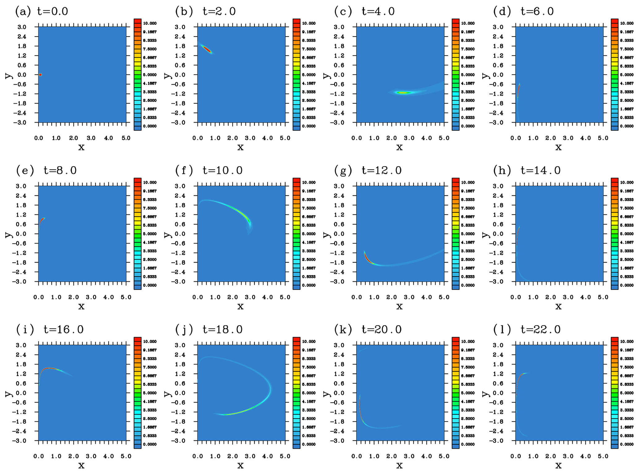
Figure 1Snapshots of the evolution of the PDF with the convective energy cycle using a direct numerical integration of the Liouville equation.
The convective energy-cycle system introduced by Yano and Plant (2012) is presented in a nondimensional form as follows:
where x is the convective kinetic energy (mass flux) and y is the cloud work function (a measure of potential energy). The equilibrium is always at and x>0.
An explicit calculation of the evolution of the initial uncertainty distribution with this system has already been performed by Yano and Ouchter (2017) using the Liouville equation. In Fig. 1 of this work, their result is reproduced in a different format compared with the original paper. Here, the initial condition is a very localized Gaussian distribution, as shown in Fig. 1a. Note that the characteristics of the subsequent evolution are qualitatively different from those of the assumed-PDF forms introduced in the following. The main challenge of the assumed-PDF approach is, nevertheless, to predict the bulk statistics of the system fairly accurately.
4.1 Combination of the gamma and the Gaussian distributions (Model I)
As the system is semi-infinite in the x direction, whereas y extends to infinity to both sides (cf. Yano and Plant, 2012), the most natural choice for the assumed-PDF form for this system, following the argument in YLP, is to adopt a gamma distribution in the x direction and a Gaussian distribution in the y direction. This is referred as Model I in the following. Thus,
where
(cf. Appendix A1). In general, the Liouville equation leads to Eq. (6); in this case, this reduces to the following:
where
By substituting Eq. (33a), (33b), (33c), and (33d) into Eq. (32), we obtain the following:
Recall that 〈 〉 suggests the phase-space average.
We are going to derive prognostic equations for the four parameters, μ, , and λi () from Eq. (34) by choosing four different weights, σ. Here, the first two only depend on x, whereas the last two only depend on y. The first two choices are σ=x and σ=x2. Substitutions of these weights into Eq. (34) lead to the following:
noting and for both σ=x and σ=x2. We have also noted the following relations:
By combining Eq. (35a) and (35b), we further obtain stand-alone prognostic equations for these two individual parameters:
Here,
To derive these three results (Eq. 36a, b, c), we have used the following relations:
Using these three relations (Eq. 36a, b, c), the right-hand side of Eq. (35c) vanishes and
whereas Eq. (35d) reduces to
As for the other two weights depending only on y, we choose and . In reductions, we invoke the following relations:
The final results are as follows:
Thus, Eq. (37a), (37b), (37c), and (37d) dictate the evolution of the distribution (Eq. 30), in which the two parameters, μ and λ2, turn out to be constants of time. On the other hand, by combining Eq. (37b) and (37c), we find
The first two terms can be rearranged to the following:
which can readily be integrated, and the trajectory of the system (noting that ) is found as follows:
where R is a constant, noting that μ is constant in time based on Eq. (37a). By comparing this final expression with Eq. (25) of Yano and Plant (2012), we find that the mean trajectory is identical to that of the solution of the system (Eq. 29a, b). Note that this is not necessarily the case. In fact, the numerical result in Fig. 2 shows that a full solution presents a damping circular trajectory in the phase space of towards the equilibrium (1,0). This aspect is simply not captured by the given assumed PDF. Thus, a remedy to it is to be sought.
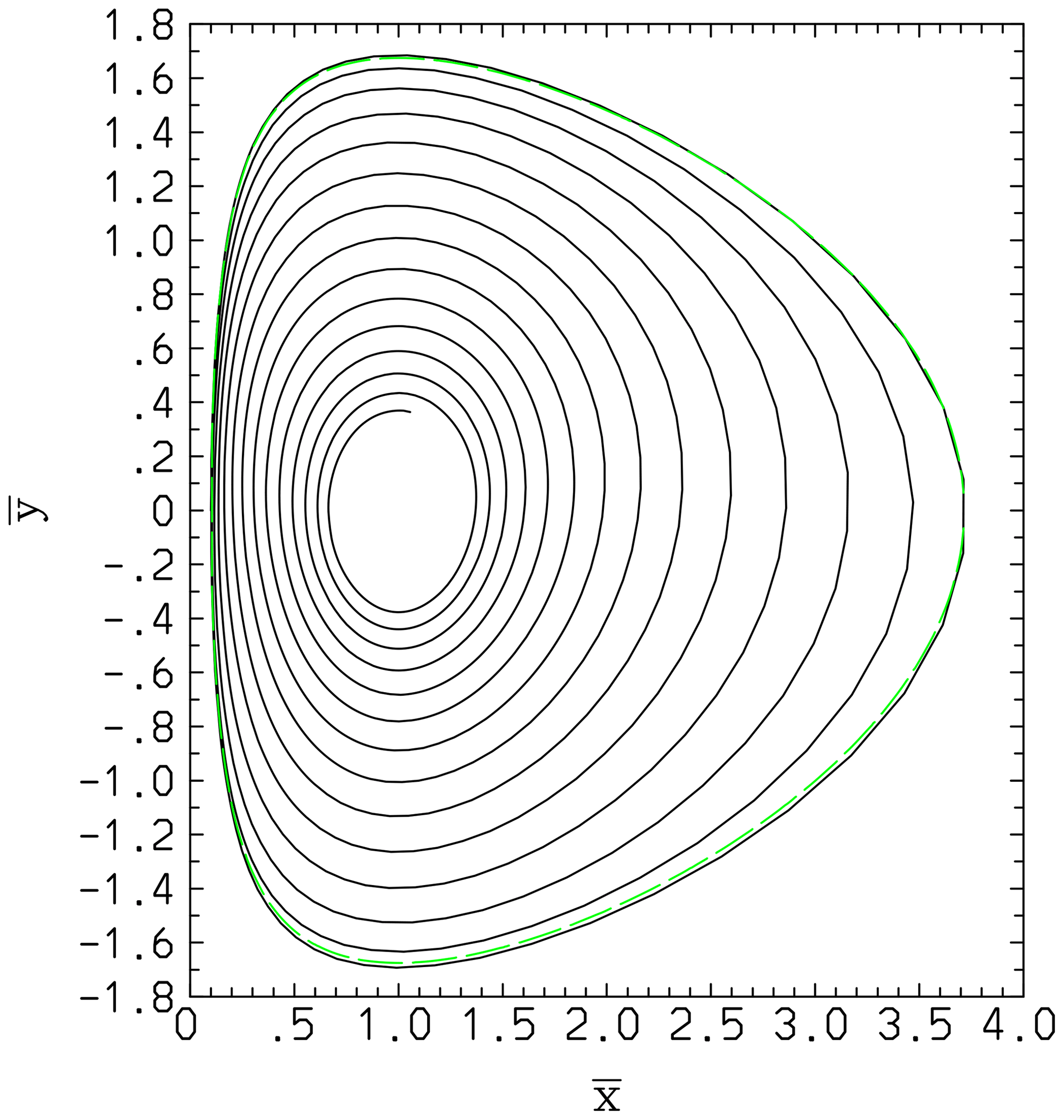
Figure 2Trajectory of as directly obtained from the Liouville equation (solid black lines) and by the assumed-PDF (Eqs. 30, 31a, b) and Model I (dashed green line) results. Here, μ=10.2271805 and R=2.19206810 in Eq. (38). This assumed-PDF solution simply takes a closed orbit, failing to reproduce the damping tendency of the actual PDF evolution.
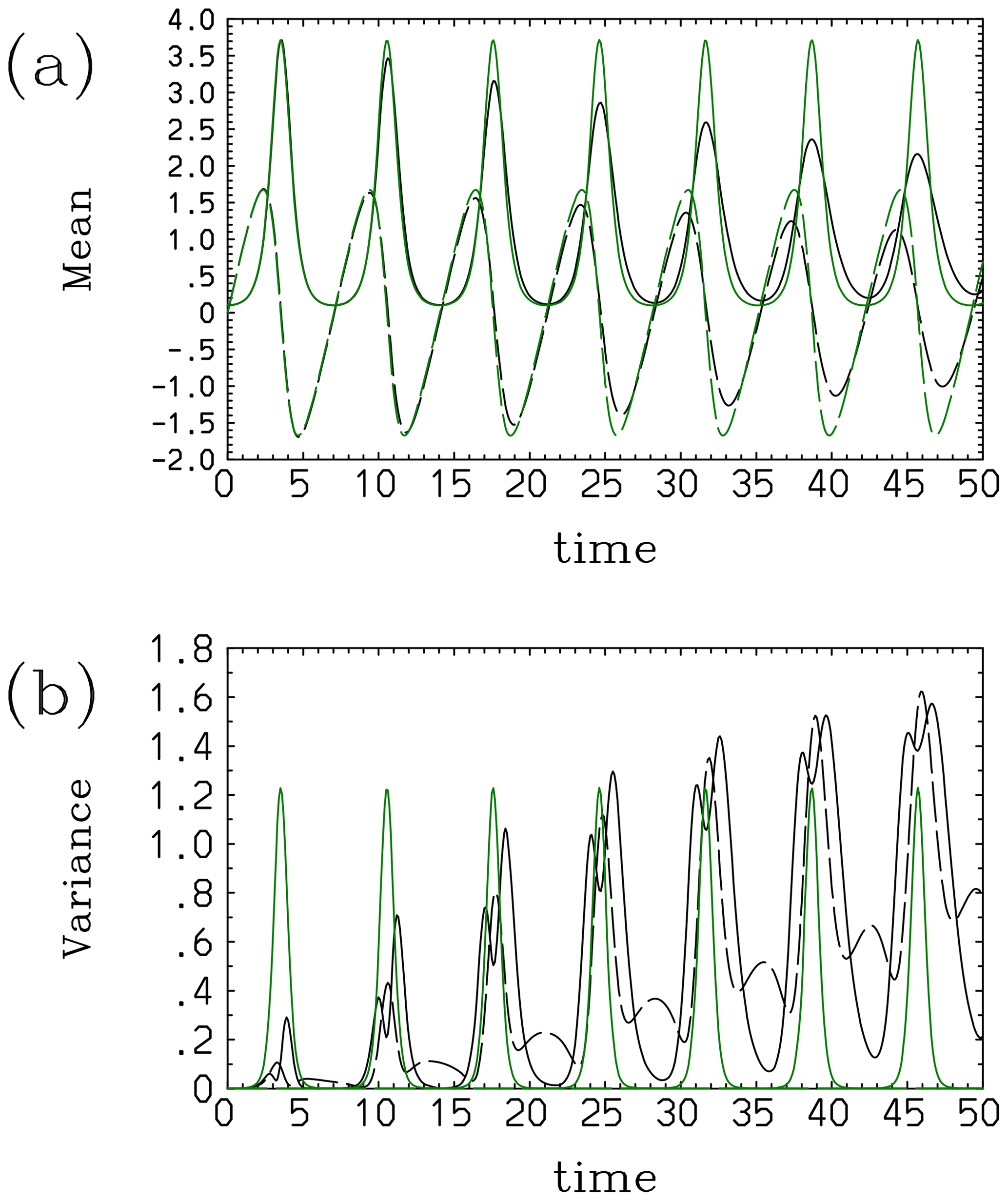
Figure 3Comparisons of the statistics of the convective energy cycle between results with a direct computation of the Liouville equation (black) and that based on the assumed-PDF method (Model I, green): (a) means, (solid line) and (long-dashed line), and (b) variances, (solid line) and (long-dashed line).
Figure 3 shows further statistical quantifications of the performance of Model I. Here, the adopted time step is . As already remarked, this model predicts a simple periodic cycle for the mean values and fails to reproduce the damping tendency of the actual PDF evolution (Fig. 3a). The same follows for the x variance (Fig. 3b), whereas Model I does not predict the evolution of the y variance – the latter is constant in time according to Eq. (37d).
An obvious defect of this assumed form is traced to the lack of correlation between the two variables, and the key nonlinear contribution, , drops out from the set of evolution equations, where and .
4.2 Two-dimensional Gaussian distribution (Model II)
Model I (Eq. 30) in the last subsection fails to predict the dissipating tendency with respect to the mean and the amplifying tendency with respect to the variance, as seen in Figs. 2 and 3. This reason for this is traced to the lack of a correlation between the two dependent variables, x and y, in the distribution; thus, the problem of the prediction of the mean becomes identical to that of the original dynamical system.
The most straightforward modification to overcome this issue is to modify the distribution as follows:
However, this assumed PDF has an unfavorable feature in that the resulting integrals become impossible to perform analytically. The requirement for numerical integrals increases the computational cost and, therefore, effectively negates the advantage of the assumed-PDF approach: an integral over an infinite domain at each time step, as required, is substantially more numerically expensive than just predicting a few PDF parameters.
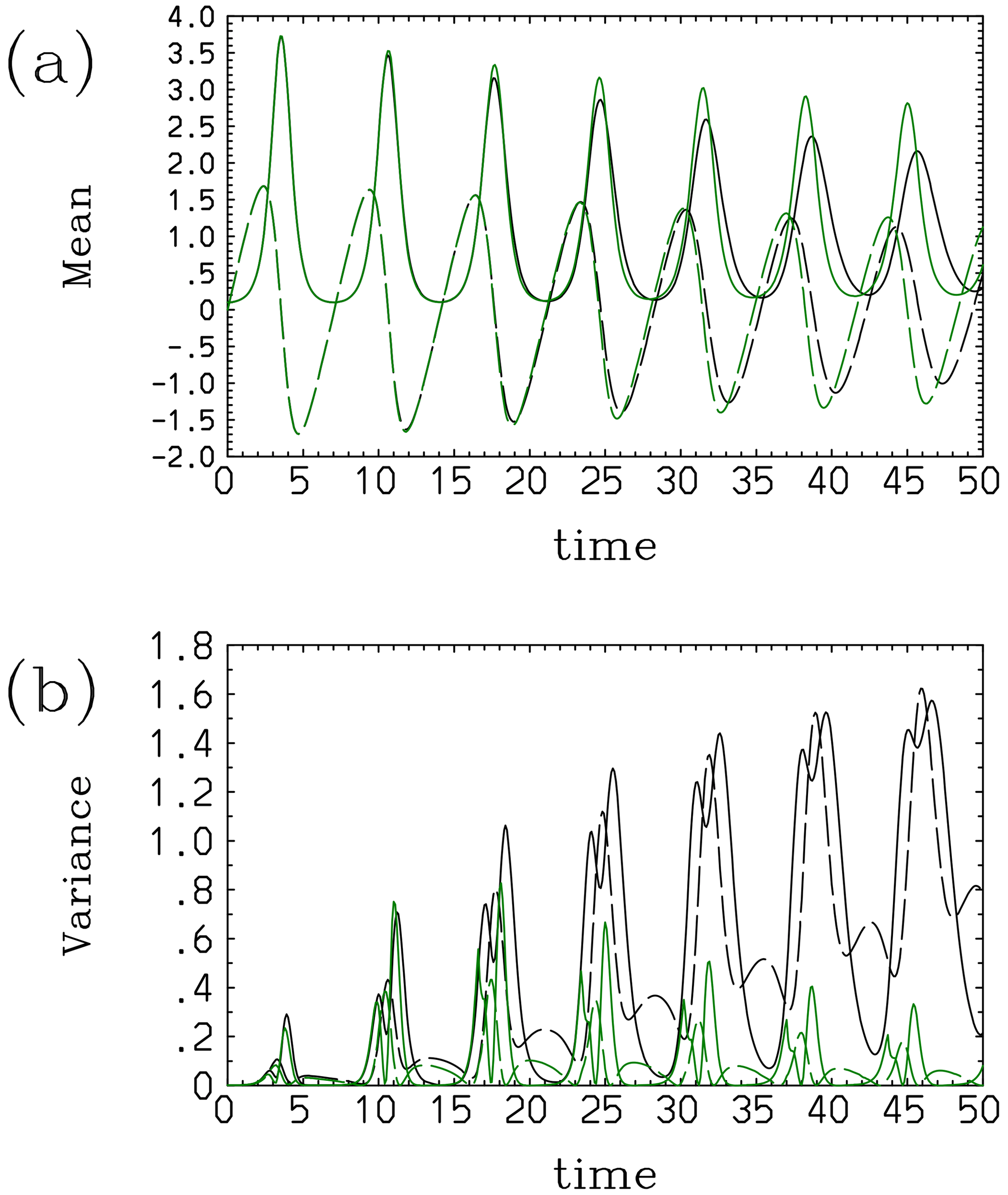
Figure 4Comparisons of the statistics of the convective energy cycle between results with a direct computation of the Liouville equation (black) and that based on the assumed-PDF method (Model II, green): (a) mean, (solid line) and (long-dashed line), and (b) variance, (solid line) and (long-dashed line).
To avoid this difficulty, we instead adopt a Gaussian distribution with the two variables considered in Sect. 3 (Eq. 21): this model is referred as Model II. A minor disadvantage with this assumed PDF is that a distribution can spread to x<0. However, this disadvantage has no serious consequence as long as we focus our attention on the basic statistics (the mean and variance, as well as correlation) and the mean of x remains positive (i.e., ).
By applying the expression of the source term for this system (Eq. 29a, b) to general formulas in Sec. 3, we obtain the following prognostic equation set for the assumed-PDF parameters:
Recall that κ is defined by Eq. (25k):
The initial condition in this case is set equal to that of the full Liouville run, which is also initialized with a Gaussian distribution.
Characteristics of the evolution of the system with Model II obtained with the time step of are shown in Fig. 4: the mean values (panel a) decay as in the case with the explicit Liouville run. The agreement is almost perfect up to the end of the third cycle, but a difference gradually becomes noticeable. A periodic increase in the variance (panel b) is also predicted up to the second cycle. However, after the end of the third cycle, the variances predicted by Model II rapidly decrease with time. The model is numerically unstable and blows up after t=60 with . Euler time-stepping is also attempted: it crashes at t=23.5. These behaviors can be understood, to a good extent, simply by inspecting the obtained prediction equations. Even using Model II, the evolution of (Eq. 39b) still follows that of y, replacing the terms by the averages, as is also the case with Model I. However, an extra term is found for the evolution equation for (Eq. 39a), which can work as a damping term whenever is satisfied, as expected from the full Liouville simulation. Due to this dissipating tendency of , also dissipates with time to the extent that the former dissipates, as seen from the long-dashed curves in Fig. 4a.
The condition is indeed satisfied initially with a Gaussian distribution leading to κ=0, with λ3=0. However, the distribution evolves with increasing κ with time, approaching κ=4. Thus, this dissipative term also becomes smaller with time, and (at a certain point) no longer dissipates as effectively as it does in the full Liouville solution, as seen from the solid curves in Fig. 4a. The variances also grow with time as long as , following Eq. (39c), (39d), and (39e). However, as remarked, due to the tendency of κ→4, this growing tendency only continues over the first three convective cycles; the variances then begin to diminish with time, as seen in Fig. 4b. These results suggest that adding a cross term (i.e., λ3≠0) in the distribution is not sufficient to reproduce statistical tendencies for an extensive duration of the simulation, especially because the variances tend to collapse after initial realistic tendencies with growing variances.
4.3 Alternative possibility
As an alternative possibility for the distributions in Sect. 4.2, the form
is also considered. As it turns out, the evolution of the mean values, and , remains identical to that of Model I without any damping tendency. A slight improvement is that the standard deviation in y, in this case, evolves with
Due to the fact that only limited improvements are expected, this case is not actually attempted. It transpires that it is crucial to include a dependence on xy in the distribution in order to successfully predict the damping tendency of mean values, as is the case with Model II.
The system proposed by Lorenz (1963) is given by the following:
Here, we assume the following standard parameters: , the Rayleigh number, r=28, and the Prandtl number, P=10. The system consists of three unstable steady solutions (i.e., fixed points): two of them corresponding to steady convection are found at , while another is found at .
First, as a reference, the evolution of the PDF is computed by directly integrating the Liouville equation. Here, the adopted numerics are identical to those used in Yano and Phillips (2016) for the Fokker–Planck equation, except that a treatment for the diffusion term arising from stochasticity is missing in the present case. The initial condition is a Gaussian distribution centered at with variances of 12.5 in all three directions. The initial center point is identical to the initial condition adopted by Lorenz (1963). An identical run has also been repeated by replacing the initial center of the Gaussian distribution to the origin, , of the system. Some remarks on this latter case will also be added in the following.
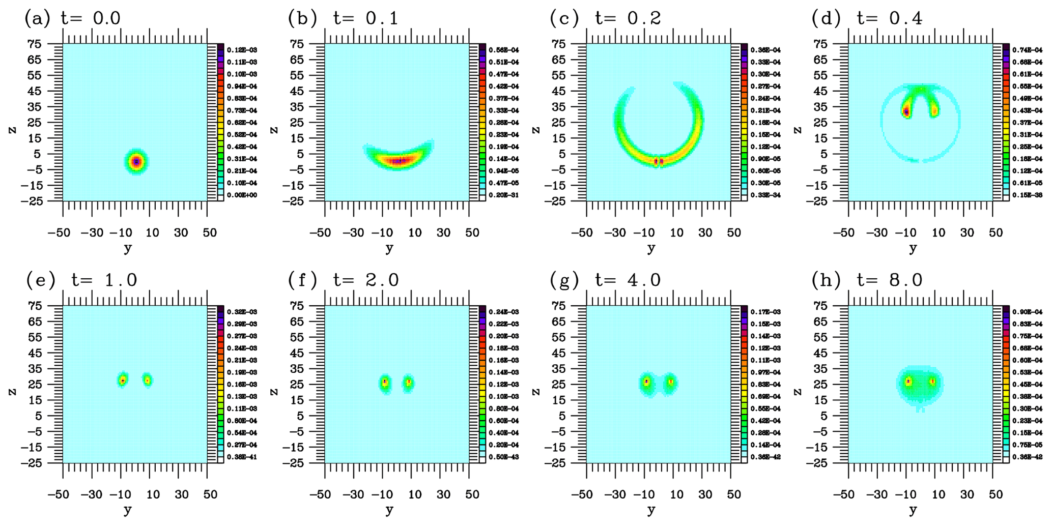
Figure 5Time evolution of the PDF for the Lorenz system on the y–z plane as directly predicted by the Liouville equation.
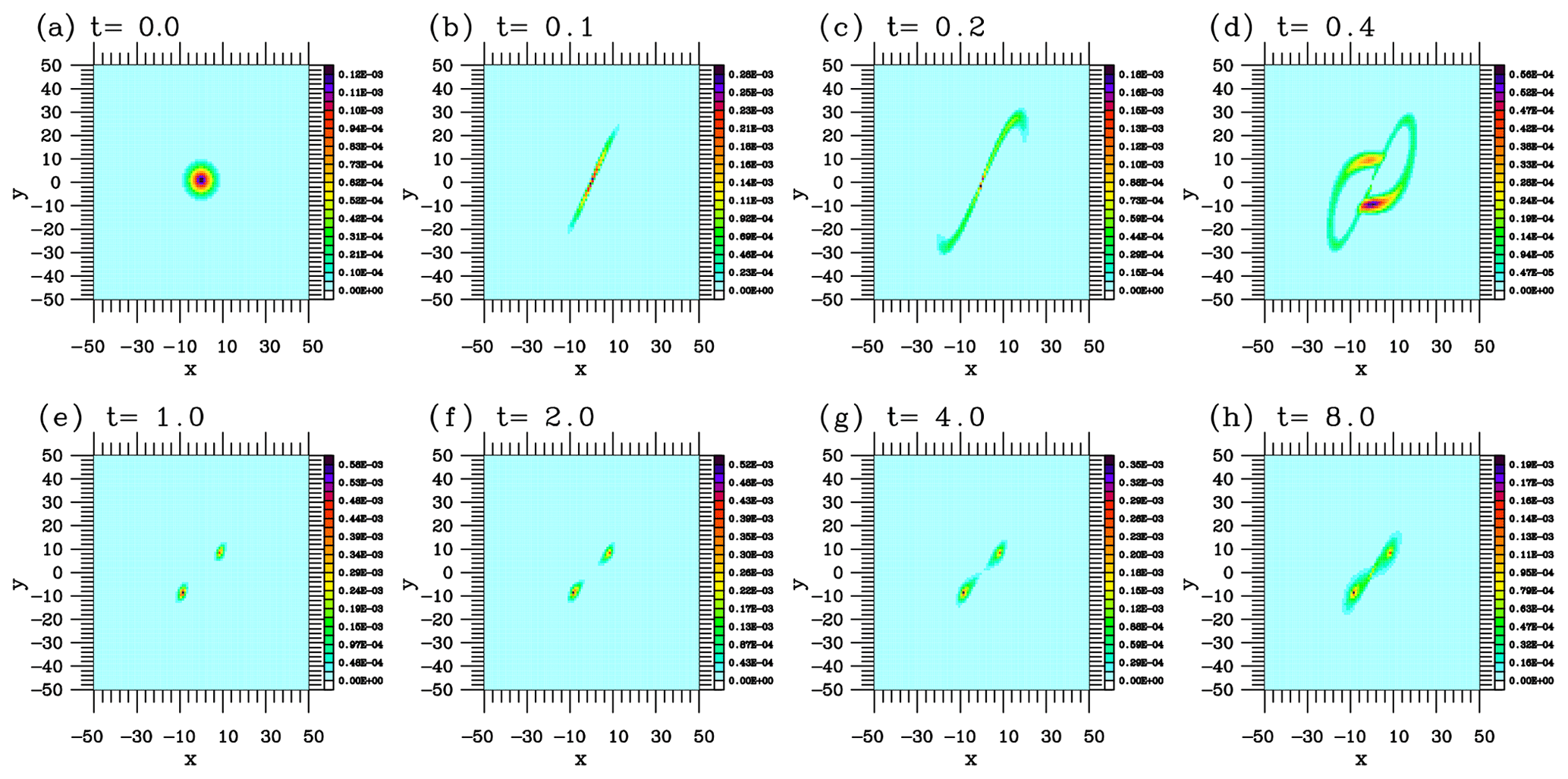
Figures 5 and 6 show that evolution of the PDF is highly non-Gaussian on both the y–z and x–y planes. On both planes, the distribution splits into two peaks over time up to t=1, corresponding to two unstable fixed points of the system. Distributions around these two peaks gradually diffuse with time as the strange attractor fully develops. Recall that the Lorenz system is chaotic; thus, the individual trajectories of solutions remain nonstationary throughout their evolution. However, as expected from the evolution of the distribution, the statistics of the system gradually converge to a stationary state after an initial transient period. Note that this is a major difference from a fully turbulent system to a low-dimensional chaotic system: in the former case, the statistics can also remain nonstationary throughout the evolution of the system. As will be demonstrated in the following, this aspect turns out to be the hardest to reproduce using an assumed-PDF form with only a few parameters, as a governing equation system predicting these PDF parameters can itself become a nonlinear chaotic system. This tendency most clearly emerges with Model I in the following.
In the following assumed-PDF demonstrations, a time step of has been adopted by default. Runs have also been repeated with , but no modification of the results has been found.
5.1 The Lorenz (1963) system: Gaussian distribution (Model I)
As the first model (Model I), we consider a three-dimensional Gaussian distribution without correlations between the dependent variables, x, y, and z:
where
Here, the normalization conditions are as follows:
where j=1, 2, 3.
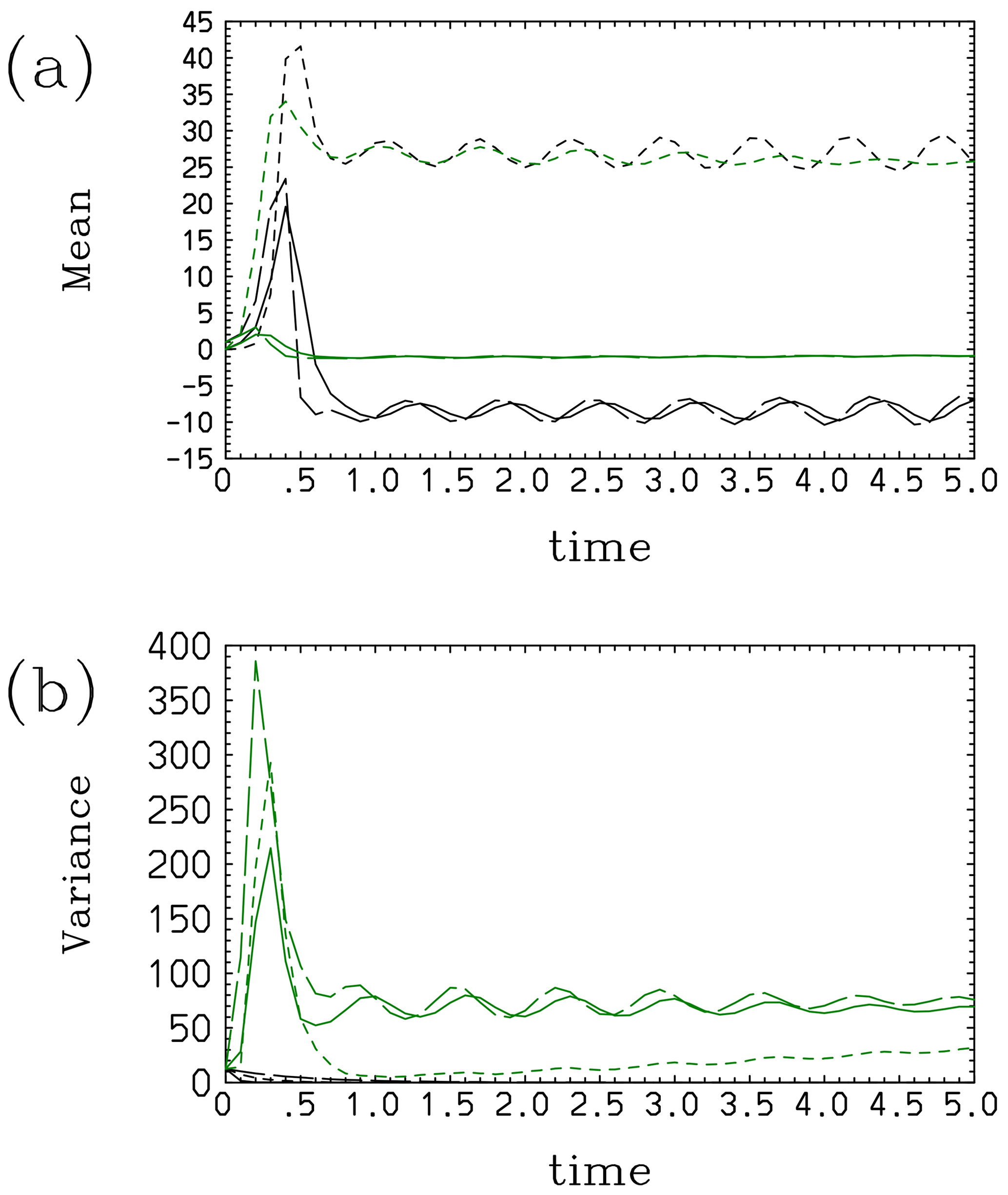
Figure 7The (a) mean and (b) variance of the Lorenz system with Model I: the model results (black) and results obtained by direct prediction with the Liouville equation (green). Here (and in the following plots), the curves are defined for the x, y, and z components using solid lines, long-dashed lines, and short-dashed lines, respectively.
From the general formulation (Eq. 6), we obtain the following:
where and σ is a weight. Moreover, we find the relations
By substituting them into Eq. (45), we find the following:
We choose the weights and (), and Eq. (47) then reduces to the following:
for j=1, 2, 3. From Eq. (41a), (41b), and (41c), the source terms are defined by
Here,
and we also find the following by direct manipulations:
Model I predicts the evolution of (short-dashed line) reasonably, but (solid line) and (long-dashed line) somehow settle to one of two unstable fixed points (to the negative side, shown in black), without suggesting an alternative possibility: equal probability among these two fixed points makes the mean values, and , close to zero in the explicit simulation (green line in Fig. 7a). Model I also fails to predict an increase in the variances at an initial phase, as seen in the explicit simulation (green line); rather, the variances simply decay rapidly (black line in Fig. 7b). The latter behavior with respect to the variances has already been seen in Eq. (48b) and the definitions (Eq. 50a, b, c) of the right-hand-side forcing term: as the parameters, λj (), are defined to be positive definite, the variance can only decay with time.
Over a longer time, the aforementioned chaotic nature of the system emerges, as shown in Fig. 8. Note especially that the equation set for the means is identical to the original Lorenz attractor system; thus, the means never converge to a statistical equilibrium, as realized in a direct computation of the Liouville equation. Instead, after t=5, the means gradually begin to oscillate around the tentatively settled unstable fixed points. A first transition happens a little after t=16, over which and transit to a nonperiodic oscillation around the origin.
5.2 The Lorenz (1963) system: semi-exponential in the y direction (Model II)
The attempt in the last subsection to constrain the system in terms of the domain-averaged statistics failed to capture the tendency of the system to settle around two unstable fixed points; rather, the assumed PDF tends to settle to only one of the two fixed points. As a measure to alleviate this tendency, we constrain the PDF in terms of the averages over subdomains of the system in this subsection. Using Model II, we now more specifically constrain the system as follows:
These constraints suggest a semi-exponential distribution in y direction:
at y=0,
Here, p1 and p3 in Eq. (42) remain the same as in Model I in Sect. 5.1.
From the normalization condition
we find
Furthermore, let
Note further,
and
The prognostic equations for λ1, , λ3, and () are as follows:
Also recall that
for j=1, 3, and further refer to Eq. (55a) and (55b). By substituting these expressions into Eq. (57a) and (57b),
When σ depends on only x or z,
The following four types of constraints (i–iv) are considered:
-
(i) ().
Here, we note as well as
for i=1 and 3. Then, we obtain
By taking a weighted sum of these expressions,
Equation (59c) predicts the evolution of with i=1, 3.
-
(ii) (). It is noted that
and we obtain
for i=1, 3. By taking the weighted sum of the two expressions,
Equation (60c) predicts the evolution of λi with i=1, 3.
Next, note that the sum over j=1, 3 drops out when σ depends only on y:
-
(iii) σ=1. Both Eq. (58a) and (58b) reduce to
where
Note that the system is overconstrained, when the σ=1 (i.e., Eq. 61) condition is used along with the results with σ=y (i.e., Eq. 62c, d). Thus, it is better not to consider the constraint (Eq. 61).
-
(iv) σ=y. Thus,
From Eq. (62a, b), we further obtain the following:
For better numerical stability, the time integration is performed in terms of , rather than . Note that both terms present a damping tendency due to the first terms on the right-hand side. Moreover, note that asymmetry arises from the second terms; thus, when tends to grow, tends to decay, and vice versa: the general tendency with this pair is qualitatively consistent with a case in which the probability of being on the positive and negative sides of y, p±, follow the evolution tendency of the individual phase-space particle. The governing equations for the parameters for the distribution in the x and z directions remain unchanged, being constrained by conditions (i) and (ii) above.
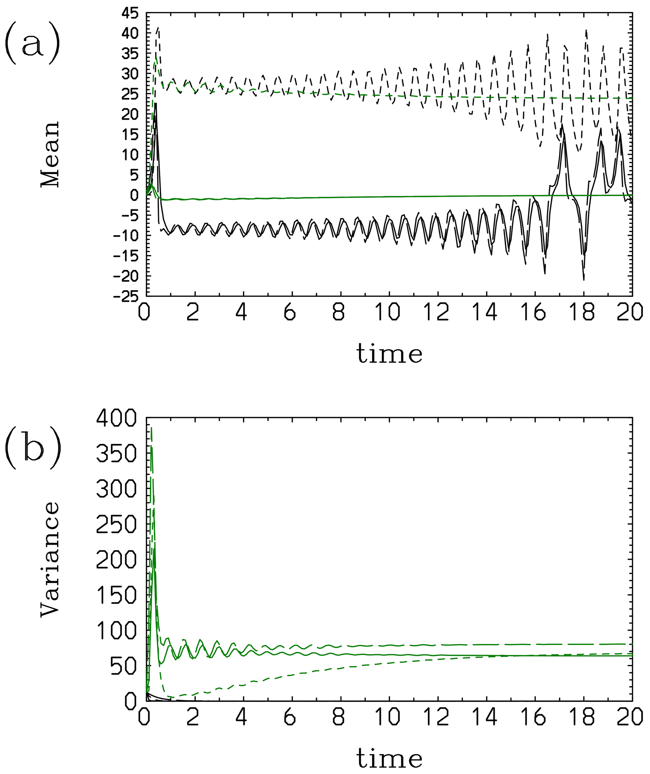
Model II shows improvement over Model I with respect to reasonably predicting the y variance (long-dashed line in Fig. 9b): it grows but with a delay of about 0.5 compared with the actual evolution directly predicted using the Liouville equation. However, as expected, prediction of the behavior of the variances of the x and z components is as unsuccessful as for Model I. The performance of x (solid line) and y (long-dashed line) for the mean (Fig. 9a) remains the same as for Model I. The failure to predict correctly, in spite of a modification of the distribution in the y direction, is attributed to the fact that the prediction of (solid line) decays to zero fairly rapidly after a relatively successful initial prediction until t≃1 (Fig. 9c). On the other hand, the prediction of (long-dashed line) is reasonable. Here, we recall the asymmetry in the initial condition.
When the run is initiated from the origin, the model behavior is even worse: both and monotonously decay towards zero with a timescale of t≃2 (not shown). Thus, the initial condition symmetric to y=0 somehow worsens the model behavior, rather than improving it; this is presumably because the first term in the right-hand sides of Eq. (62c) and (62d) dominate throughout the experiment.
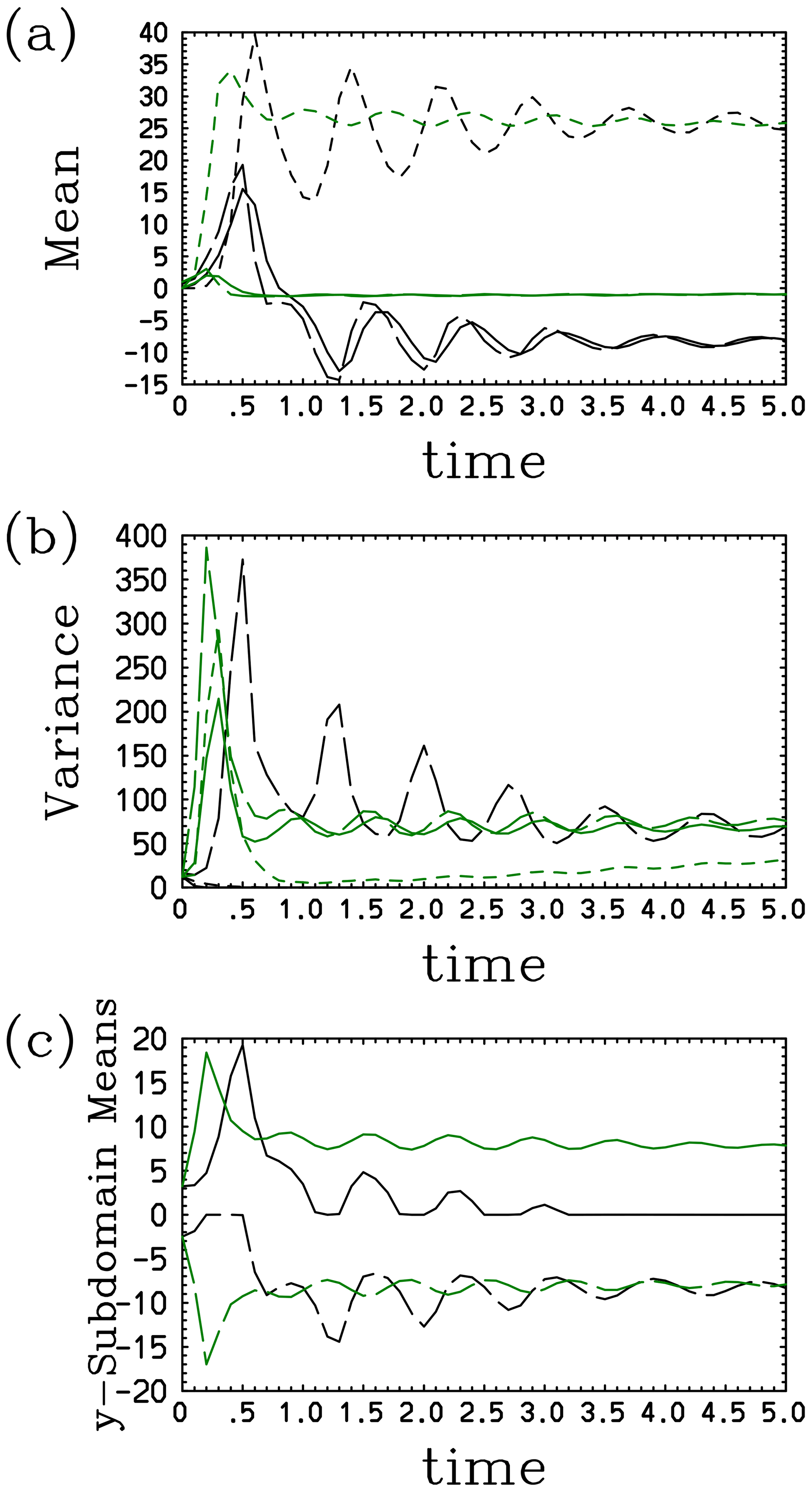
Figure 9The (a) mean, (b) variance, and (c) (solid line) and (long-dashed line) of the Lorenz system with Model II: the model results (black) and results obtained by direct prediction with the Liouville equation (green). In panels (a) and (b), the solid, long-dashed, and short-dashed curves denote the respective x, y, and z components.
5.3 The Lorenz (1963) system (Model III)
As a further extension of Model II in the last subsection, we now also constrain the system by . In this case, p1 takes the following form:
Derivation of the equations for the assumed-PDF coefficients also proceeds in a similar manner to that outlined in the last subsection; the only change is that the terms are now predicated by
The major improvement with this modification is better performance with respect to the x variance (solid line in Fig. 10b): it no longer decays out rapidly; rather, it remains about one-half of the actual value. On the other hand, the performance of the z variance (short-dashed line in Fig. 10b) does not change. As a rather intriguing modification, both (solid line) and (long-dashed line) somehow settled to a positive unstable fixed point in this case (Fig. 10a).
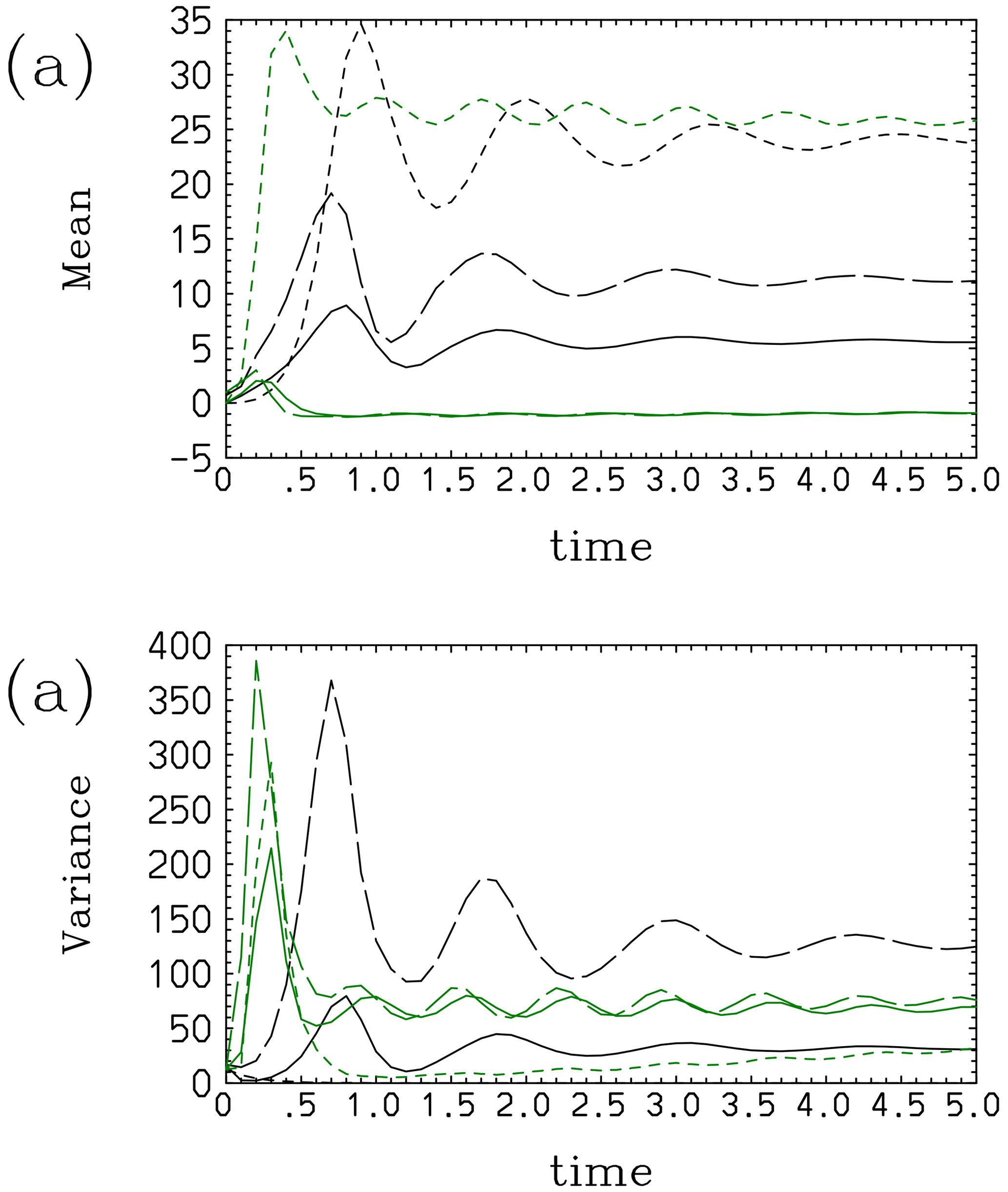
Figure 10The (a) mean and (b) variance of the Lorenz system with Model III: the model results (black) and results obtained by direct prediction with the Liouville equation (green).
Even after the attempts with these three assumed PDFs, a successful representation of the statistics associated with a split of the distribution into two peaks is still a key remaining challenge. However, as it currently stands, it is not clear which parameter should be added to satisfy this challenge.
A general methodology for solving the time evolution of assumed-PDF parameters based on the Liouville equation has been proposed by Yano et al. (2024), with this prior study referred to as YLP in this work. The present paper extends this study in several aspects. First, it has been generalized (Sect. 2.2) for cases in which the constraints are defined by limited integral ranges. This generalization is a critical first step, for example, in developing a cloud scheme based on this formulation. As a result, the assumed-PDF forms also take different forms over different subdomains; thus, hereafter, the formulation for the prognostic equations for the PDF parameters has also been generalized accordingly (Sect. 2.3). Finally, the formulation has been explicitly generalized into multidimensional cases (Sect. 2.4 and 2.5). These further generalized formulations have been applied to two simple dynamical systems (Sects. 4 and 5, respectively): a convective energy-cycle system proposed by Yano and Plant (2012) and the Lorenz (1963) strange-attractor system.
Here, it may be worthwhile reiterating the originality of the present study, as extensive work already exists within the framework of the so-called assumed-PDF approach. In fact, as emphasized in YLP, more or less all of the existing formulations for the distribution problems fall into this category. However, this work is original in that it attempts to predict the evolution of a distribution in a self-consistent manner and to verify the performance using simple dynamical systems. Such an effort does not exist in the literature, as the existing assumed-PDF schemes, both with respect to subgrid-scale representations and cloud microphysics, are developed case by case with ad hoc closures, without generality. Thus, it is simply not possible to perform verifications of those schemes using simple dynamical systems.
The performance of the assumed-PDF formulations has been directly compared with the results from the direct time integration of the Liouville equation for both systems. By adopting simple dynamical systems with up to three dependent variables, such direct time integration becomes feasible. Unfortunately, both testing cases tend to suffer from the same tendencies: regardless of a specific choice, statistics (means and variances) predicted by an assumed-PDF approach gradually noticeably deviate from the exact results predicted by the Liouville equation. Furthermore, some statistics, for example, the sign-dependent conditional averages, and , in the Lorenz system turn out to be rather difficult to predict properly: in general, only one of the sign-dependent mean pair, , is predicted properly, and the other of the pair simply settles to a vanishing value. In this respect, the assumed-PDF approach does not provide a “magic recipe”.
One may judge that the obtained results are not overly promising and, perhaps, even a failure. However, it should be emphasized that rather difficult cases are used as test cases: for both systems, the initial Gaussian distribution rapidly evolves into a qualitatively totally different form. One must also consider the more basic fact that the assumed PDF attempts something almost impossible: performing an accurate prediction of a distribution by only using a limited number of parameters. For this reason, one should consider the obtained results an important demonstration of the fundamental difficulties associated with assumed-PDF methods in general, not only with the particular approach adopted herein. Arguably, the performance is rather impressive considering the fact that the PDF forms assumed are also qualitatively very different from the actual distributions predicted by the Liouville equation. The real question still to be to answered is how well the more standard assumed-PDF approaches perform with the same systems. In that manner, the advantage of the present assumed-PDF approach may be better established.
The study has also suggested that the output-constrained distribution principle, proposed by YLP, may not be sufficient to decide an assumed-PDF form: to ensure good performance of a prediction of the distribution statistics, assumed-PDF forms must be constrained by something more than just those required as outputs for host models. In the present study, we have assumed that those constraints should be averages and variances. The present exploratory study has suggested that it is also crucial to evaluate the mean evolution of actual forcing terms of a system accurately; thus, they must also be added as a constraint. In both of the models considered herein, the term xy is crucial in prediction; thus, this correlation term must also be properly predicted. It has been shown that adding a constraint of 〈xy〉 can improve the predictions by assumed-PDF forms, although not necessarily in a satisfactory manner.
Prediction of the PDF of the Lorenz system is inherently difficult due to the fact that the solution tends to be clustered around the two unstable fixed points. The assumed-PDF, with all of the cases considered so far, have always failed to predict one of those two tendencies under conditional averages, and . A further possibility to pursue is to re-initialize a prediction at a middle point, in the spirit of data assimilation, and to examine whether this difficulty is overcome by this procedure.
Some numerical issues have also been revealed by the present study. In some cases, exponential parameters in a distribution can vary to extremes that cause overflow and underflow problems in computations. To avoid this issue, some exponential parameters have been predicted in their logarithmic form to ensure better numerical stability. However, these basic procedures have not always been able to resolve the stability issues: in the case of Model III for the Lorenz system (Sect. 5.3), a rather small nondimensional time step of 10−4 has been necessary to run a prediction for long enough, but it still ultimately crashes. The numerical stability of this case must more closely be investigated in its own right.
As a whole, the present study reveals the inherent difficulties associated with accurately predicting a distribution with a limited number of distribution parameters. In particular, we have faced the universal tendency of the variance of the distribution to decay with time, when it must increase, regardless of the choice of the assumed distribution form. This behavior is reminiscent of the variance collapse identified as a major problem in data assimilation when it is performed with an ensemble. In the latter case, it is often found that the probability weight assigned to each ensemble member collapses close to zero except for a single member close to the average (i.e., weight collapse; see van Leeuwen, 2003, and Poterjoy, 2016); thus, the prior estimate of the variance also collapses as a consequence (cf. Snyder et al., 2008; the reader is referred to van Leeuwen, 2009, for more background). Although the cause of this problem is usually attributed to a relatively small ensemble size and the tendency of the ensemble to collapse into a “stable” state, the present study suggests that this tendency is more universal, and it can happen whenever a highly truncated representation of a distribution is adopted, even with an approach considering a full dimension of the phase space, as in the present case.
These ensemble-based assimilation studies, in turn, have attempted various remedies to alleviate this tendency: the simplest is to inflate the variance by a certain factor with time to prevent its collapse (Anderson and Anderson, 1999; Anderson, 2001). More generally, resampling approaches can, at least, partially delay the collapse of the weights (Snyder et al., 2008; Anderson, 2001). However, it appears that neither of the approaches is directly applicable to the assumed-PDF formulation in the present study. First, the inflation is nothing other than adding an extra adjustable parameter, which can only be chosen when an exact PDF evolution is known a priori. Resampling approaches do not work by simply not adopting an ensemble formulation.
The most feasible solution to solve the variance collapse under the assume-PDF approaches would be to include a feedback of the truncated distribution parameters in the form of a parameterization, in a similar manner to that with which the effects of higher moments are represented by certain hypotheses in the turbulence-closure models (Mellor, 1973; Mellor and Yamada, 1974). However, parameterization of the higher-order assumed-PDF parameters is a completely new frontier, and much investment is required before we can propose any specific solution.
A1 Normalization
The normalization condition for a distribution with two variables, (x,y), is given by
Recall the Gaussian integral formula
For casting the integral in x in this form, we rearrange a part of the exponent as follows:
Thus,
The remaining exponent can be rearranged as
Thus, a further integral of Eq. (A1) in y leads to
The final expression proves Eq. (31a), (31b), and (31c).
A2 Moments
The moments given by Eq. (25a)–(25j) are derived using relationships obtained by taking the differentiation of the Gaussian distribution in a recursive manner:
The integral of the right-hand side leads to
This relation immediately finds the following:
Likewise, by symmetry
Solving these expressions together leads to Eq. (25a), provided .
To generalize a type of relation like Eq. (A3a) and (A3b), we note that Eq. (A2) is still valid by multiplying a weight, σ, by any function of y. Letting ,
By symmetry,
By combining these expressions together, we obtain the following relations:
Equation (A2) can further be used to derive similar expressions for higher-moment integrals:
where n is an arbitrary integral. We first set n=2 and then obtain the following by a partial integral:
Thus,
As the partial integral vanishes, by expanding the left-hand side, we obtain
By symmetry, we also obtain
By substituting Eq. (A5b) and (A5c) into the above, we obtain Eq. (25d). Its substitution back to Eq. (A5b) and (A5c) leads to Eq. (25b) and (25c), respectively.
To obtain the expressions for the third moments, we now set n=3 in Eq. (A6). As this whole integral vanishes, by expanding this integral, we obtain the following:
By symmetry,
As an extension of Eq. (A3a) and (A3b), we obtain the following:
They lead to the following:
By substituting Eq. (A9a) and (A9b) into Eq. (A8a) and (A8b), we obtain
By solving them for and and also substituting this result into Eq. (A9a) and (A9b), we obtain Eq. (25e).
Finally, to obtain the results for the fourth moments, we set n=4 in Eq. (A6), which leads to the following:
By symmetry,
As an extension of Eq. (A3a) and (A3b), we obtain
which lead to
The results of Eq. (A7a) and (A7b) are extended by applying weights of and , respectively, and we obtain the following:
By substituting Eq. (A11a) and (A11b) into the above, we obtain the following:
We first substitute Eq. (A11a) and (A11b) into Eq. (A10a) and (A10b) and then substitute Eq. (A12a) and (A12b) into the latter. This gives Eq. (25h). Substituting Eq. (25h) back into Eq. (A12a) and (A12b) gives Eq. (25f) and (25g), and further substitutions of them into Eq. (A11a) and (A11b) lead to Eq. (25i) and (25j).
The Fortran codes used in the present study are available from the author upon request.
No data sources were used in the present study.
The author has declared that there are no competing interests.
Publisher’s note: Copernicus Publications remains neutral with regard to jurisdictional claims made in the text, published maps, institutional affiliations, or any other geographical representation in this paper. While Copernicus Publications makes every effort to include appropriate place names, the final responsibility lies with the authors.
The present work has evolved over years via discussions with various people, but extensive discussions with Vince Larson and Vaughan Phillips are particularly acknowledged.
This paper was edited by Natale Alberto Carrassi and reviewed by two anonymous referees.
Anderson, J. L.: An ensemble adjustment Kalman filter for data assimilation, Mon. Weather Rev., 129, 2084–2903, 2001. a, b
Anderson, J. L. and Anderson, S. L.: A Monte-Carlo implementation of the nonlinear filtering problem to produce ensemble assimilations and forecasts, Mon. Weather Rev., 127, 2741–2758, 1999. a
Bechtold, P., Fravalo, C., and Pinty, J. P.: A model of marine boundary-layer cloudness for mesoscale applications, J. Atmos. Sci., 49, 1723–1744, 1992. a
Bechtold, P., Cuijpers, J. W. M., Mascart, P., and Trouilhet, P.: Modeling of trade-wind cumuli with a low-order turbulence model – Towards a unified description of Cu and Sc clouds in meteorological models, J. Atmos. Sci., 52, 455–463, 1995. a
Bony, S. and Emanuel, K. A.: A parameterization of the cloudness associated with cumulus convection: Evaluation using TOGA COARE data, J. Atmos. Sci., 58, 3158–3183, 2001. a
Bougeault, P.: Modeling the trade-wind cumulus boundary-layer. Part I: Testing the ensemble cloud relations against numerical data, J. Atmos. Sci., 38, 2414–2428, 1981. a
Carrassi, A., Bocquet, M., Bertino, L., and Evensen, G.: Data assimilation in the geosciences: An overview of methods, issues, and perspectives, Climatic Change, 9, e535, https://doi.org/10.1002/wcc.535, 2018. a
Evensen, G., Vossepoel, F. C., and van Leeuwen, P. J.: Data Assimilation Fundamentals, Springer, Berlin, 246 pp., ISBN-10 3030967085, 2022. a
Golaz, J.-C., Larson, V. E., and Cotton, W. R.: A PDF-based model for boundary layer clouds. Part I: Method and model description, J. Atmos. Sci., 59, 3540–3551, 2002. a, b, c
Khain, A. P. and Pinsky, M.: Physical Processes in Clouds and Cloud Modeling, Cambridge University Press, Cambridge, 626 pp., ISBN 0521767431, 9780521767439, 2018. a
Khain, A. P., Beheng, K. D., Heymsfield, A., Korolev, A., Krichak, S. O., Levin, Z., Pinsky, M., Phillips, V., Prabhakaran, T., Teller, A., van den Heever, S. C., and Yano, J. I.: Representation of microphysical processes in cloud-resolving models: spectral (bin) microphysics vs. bulk-microphysics, Rev. Geophys., 53, 247–322, https://doi.org/10.1002/2014RG000468, 2015. a
Larson, V. E. and Golaz, J.: Using probability density functions to derive consistent closure relationships among higher-order Moments, Mon. Weather Rev., 133, 1023–1042, https://doi.org/10.1175/MWR2902.1, 2005. a
Le Treut, H. and Li, Z. X.: Sensitivity of an atmospheric general circulation model to prescribed SST changes: Feedback effects associated with the simulation of cloud optical properties, Clim. Dynam., 5, 175–187, 1991. a
Lorenz, Z. N.: Deterministic nonperiodic flow, J. Atmos. Sci., 20, 130–141, 1963. a, b, c, d, e, f, g, h
Mellor, G. L.: Analytic prediction of the properties of stratified planetary surface layers, J. Atmos. Sci., 30, 1061–1069, 1973. a
Mellor, G. L.: Gaussian cloud model relations. J. Atmos. Sci., 34, 356–358, 1977. a
Mellor, G. L. and Yamada, T.: A hierarchy of turbulence closure models for planetary boundary layers, J. Atmos. Sci., 31, 1791–1806, 1974. a
Poterjoy, J.: A localized particle filter for high-dimensional nonlinear systems, Mon. Weather Rev., 144, 59–76, 2016. a
Richard, J. L. and Royer, J. F.: A statistical cloud scheme for ruse in an AGCM, Ann. Geophys., 11, 1095–1115, 1993. a
Snyder, C., Bengtsson, T., Bickel, P., and Anderson, J.: Obstacles high-dimensional particle filtering, Mon. Weather Rev., 136, 4629–4640, 2006. a, b
Sommeria, G. and Deadorff, J. W.: Subgrid-scale condensation in models of nonprecipitating clouds, J. Atmos. Sci., 34, 344–355, 1977. a
Tompkins, A. M.: A prognostic parameterization for the subgrid-scale variability of water vapor and clouds in large-scale models and its use to diagnose cloud cover, J. Atmos. Sci., 59, 1917–1942, 2002. a
van Leeuwen, P. J.: A variance -minimizing filter for large-scale applications, Mon. Weather Rev., 131, 2071–2084, 2003. a
van Leeuwen, P. J.: Particle filtering in geophysical systems. J. Climate, 137, 4089–4114, 2009. a
Yano, J.-I. and Ouchtar, E.: Convective Initiation Uncertainties Without Trigger or Stochasticity: Probabilistic Description by the Liouville Equation and Bayes' Theorem, Q. J. Roy. Meteor. Soc., 143, 2015–2035, https://doi.org/10.1002/qj.3064, 2017. a
Yano, J.-I. and Phillips, V. T. J.: Explosive ice multiplication induced by multiplicative-noise fluctuation of mechanical break-up in ice-ice collisions, J. Atmos Sci., 73, 4685–4697, 2016. a
Yano, J.-I. and Plant, R. S.: Finite Departure from Convective Quasi-Equilibrium: Periodic Cycle and Discharge-Recharge Mechanism, Q. J. Roy. Meteor. Soc., 138, 626–637, 2012, https://doi.org/10.1002/qj.957. a, b, c, d, e, f, g
Yano, J.-I., Ziemiański, M., Cullen, M., Termonia, P., Onvlee, J., Bengtsson, L., Carrassi, A., Davy, R., Deluca, A., Gray, S. L., Homar, V., Köhler, M., Krichak, S., Michaelides, S., Phillips, V. T. J., Soares, P. M. M., and Wyszogrodzki, A.: Scientific Challenges of Convective-Scale Numerical Weather Prediction, B. Am. Meteorol. Soc., 99, 699–710, https://doi.org/10.1175/bams-d-17-0125.1, 2018. a
Yano, J.-I., Larson, V., and Phillips, V. T. J.: Technical Note: General Formulation For the Distribution Problem: Prognostic Assumed PDF Approach Based on The Maximum–Entropy Principle and The Liouville Equation, EGUsphere [preprint], https://doi.org/10.5194/egusphere-2023-2278, 2024. a, b
- Abstract
- Introduction
- General formulation
- Example: Gaussian distribution with two variables
- Convective energy-cycle system (Yano and Plant, 2012)
- The Lorenz (1963) system
- Summary and discussions
- Appendix A: Integrals of the two-dimensional Gaussian distribution
- Code availability
- Data availability
- Competing interests
- Disclaimer
- Acknowledgements
- Review statement
- References