the Creative Commons Attribution 4.0 License.
the Creative Commons Attribution 4.0 License.
 | 12 Jul 2024
Bridging classical data assimilation and optimal transport: the 3D-Var case
Pierre J. Vanderbecken
Alban Farchi
Joffrey Dumont Le Brazidec
Yelva Roustan
Because optimal transport (OT) acts as displacement interpolation in physical space rather than as interpolation in value space, it can avoid double-penalty errors generated by mislocations of geophysical fields. As such, it provides a very attractive metric for non-negative, sharp field comparison – the Wasserstein distance – which could further be used in data assimilation (DA) for the geosciences. However, the algorithmic and numerical implementations of such a distance are not straightforward. Moreover, its theoretical formulation within typical DA problems faces conceptual challenges, resulting in scarce contributions on the topic in the literature.
We formulate the problem in a way that offers a unified view with respect to both classical DA and OT. The resulting OTDA framework accounts for both the classical source of prior errors, background and observation, and a Wasserstein barycentre in between states which are pre-images of the background state and observation vector. We show that the hybrid OTDA analysis can be decomposed as a simpler OTDA problem involving a single Wasserstein distance, followed by a Wasserstein barycentre problem that ignores the prior errors and can be seen as a McCann interpolant. We also propose a less enlightening but straightforward solution to the full OTDA problem, which includes the derivation of its analysis error covariance matrix. Thanks to these theoretical developments, we are able to extend the classical 3D-Var/BLUE (best linear unbiased estimator) paradigm at the core of most classical DA schemes. The resulting formalism is very flexible and can account for sparse, noisy observations and non-Gaussian error statistics. It is illustrated by simple one- and two-dimensional examples that show the richness of the new types of analysis offered by this unification.
- Article
(4603 KB) - Full-text XML
- BibTeX
- EndNote


1.1 Data assimilation and the double-penalty issue
Geophysical data assimilation (DA) is a set of methods and algorithms at the intersection of Earth sciences, mathematics, and computer science that are designed to enhance our understanding and predictive capability with respect to the complex systems that govern our planet (Carrassi et al., 2018). For example, these systems encompass the atmosphere, ocean, atmospheric chemistry and biogeochemistry, land surfaces, glaciology, hydrology, and climate system as a whole. DA is meant to optimally combine all sources of quantitative information, typically past and present observations, and numerical and statistical models of the system under consideration. DA is critical in forecasting chaotic geofluids by resetting the initial conditions of the flow, estimating physical and statistical parameters of the models, and providing a quantitative reanalysis of the past history of the climate system over decades. Because classical DA is applied to complex and high-dimensional dynamics, the DA algorithms often result from a compromise between the sophistication of the employed mathematical techniques and their numerical scalability and efficiency (Kalnay, 2003; Asch et al., 2016; Evensen et al., 2022). For instance, it is well-known that most DA methods are built around or from an update step – the analysis – where observations and background states are combined, an operation which often relies on Gaussian statistical assumptions.
Here, we would like to focus on one important issue that impacts classical DA, known as the double-penalty error in the geosciences. The double-penalty issue refers to the over-penalisation of errors in both the model and observational data (e.g. Amodei and Stein, 2009) and compromises the balance required for effective DA. It often stems from the mislocation of fields, which is caused by model error in either the forecasting or observation operator. A typical example is given by the slight mislocation of a plume of pollutant resulting in high predicted concentration values at positions where no pollutant is observed, while the model misses the observed concentration peaks (Farchi et al., 2016). This mismatch is heavily penalised due to the use, over the same discretised space, of the root-mean-square error (RMSE) for a point-by-point comparison. Figure 1 shows an exemplar of double-penalty error resulting in the inability to properly evaluate a model and learn from an analysis increment. This double-penalty error, a very common contribution to the representation error (Janjić et al., 2018), is ubiquitous in the geosciences, for example, in numerical weather prediction (in particular for water vapour), in atmospheric chemistry and air quality, in biogeochemistry, and in eddy-resolving ocean forecasting. This especially applies to sharp fields, whereas it may be of less relevance for smoother, larger-scale fields such as temperature.
Figure 1 These two panels schematise the computation of the RMSE of two analysis increments. These increments are the difference between the truth (left mesh in between both pairs of the norm delimiters), concentrated here in the red grid cell, and the analysis, located in the green grid cells (right mesh in between both pairs of the norm delimiters). The increment in panel (a) is the outcome of a better analysis that is spatially closer to the truth, compared with that in panel (b); however, both increments yield the same RMSE. Hence, this verification metric is impacted by the double-penalty error and does not help discriminate location errors.
It has been recognised that, although it can handle amplitude and smoothness mismatch, the weighted Euclidean (Mahalanobis) distance cannot cope with mislocation error; thus, it cannot account for the full distortion between mismatched fields (Hoffman et al., 1995). In the field of precipitation verification, one would alternatively speak of amplitude, structure, and location errors (e.g. Wernli et al., 2008). Hence, even though tuning covariances of Gaussian error distributions as in classical DA, such as increasing the correlation length, might help mitigate the double-penalty error, it is insufficient. In Fig. 1, one might replace the Euclidean norm with a weighted Euclidean one with a large correlation length. This would yield similar norm values for both cases. Unfortunately, it is not difficult to show that, in this limit, this (almost singular) norm can only distinguish between the spatial mean of both fields: it became blunt with no discriminating power. With respect to DA, Feyeux et al. (2018, their Fig. 1) also illustrate why the Euclidean distance cannot properly cope with mislocation error. Note that, if Feyeux et al. (2018) had used a weighted Euclidean distance instead, with the same covariance matrix for the two contributions of the cost function, the resulting analysis state would have been the same and, in particular, independent of the covariance matrix. A similar but two-dimensional illustration is given by Vanderbecken et al. (2023, their Fig. 3).
1.2 Nonlocal verification metrics
The issue can be attributed to the use of a local verification metric, meaning that it compares, through the RMSE, values at the same site, of the same grid cell. Thus, this issue goes beyond DA and pertains to the use of local metrics.
To avoid being impacted by the double-penalty issue stemming from the use of local verification metrics, smarter nonlocal or multiscale metrics have been proposed. A typical metric of this kind consists of the combination of a displacement map followed by the use of classical norm such as the RMSE (Hoffman et al., 1995; Keil and Craig, 2009). In this vein, effective verification metrics can be based on optical flow-based warping or on deformed meshes, prior to using classical norms (Gilleland et al., 2010a, b). These metrics can also be designed as scale-dependent and possibly multiscale, based on an empirical separation of scales, such as with fuzzy metrics (Ebert, 2008; Amodei and Stein, 2009) or wavelets (Briggs and Levine, 1997). They can be designed to grasp and quantify objects and features, such as lows and highs (Davis et al., 2006a, b; Lack et al., 2010). Metrics with similar capabilities (but not necessarily based on a displacement concept) have been introduced in computer vision, such as the structural similarity index (Zhou et al., 2004), or in the verification of precipitation (Wernli et al., 2008; Skok, 2023; Necker et al., 2023).
One of the most elegant approaches is based on the theory of optimal transport (OT) and the associated Wasserstein distance, which sits on solid mathematical foundations and significant developments; these are the main reasons why we will focus on OT in the following. Examples of the application of OT to the verification of tracer and greenhouse gases models are given in Farchi et al. (2016) and Vanderbecken et al. (2023).
1.3 Optimal transport and the Wasserstein distance
Before mentioning applications of the Wasserstein distance in the field of geoscience, let us first give a very brief introduction to the concept and mathematical formulation of OT.
Figure 2 Illustration of the earth mover problem introduced by Monge in 1781 (see bulk of paper).
The OT concept stems from an engineering, although rather universal, problem. Gaspard Monge (Monge, 1781) considered the earth mover problem, the goal of which is to efficiently move rubble to an embankment of about the same volume (see Fig. 2). Each displacement of a bit of earth has a known cost, so that the goal is to find the cheapest deterministic map that completely moves the rubble to the embankment. In mathematical terms, the goal is to find the map of minimal cost that transports the origin measure ρo to the target measure ρb; measure here means that both of them are non-negative and are integrable of integral 1. Note that the value 1 is arbitrary here and can be changed to m>0, provided that this is the mass of both ρo and ρb. The cost is defined by a non-negative function 𝒞bo of two variables (one for the origin space and the other for the target space). Let us assume a quadratic cost, defined for any couple of points (x,y) of a geometric domain Ω:
where ∥⋅∥2 is the Euclidean norm. Let us define the set of all admissible differentiable maps T that transport ρo to ρb:
where |∂xT| is the absolute value of the determinant of the Jacobian of T, a factor which accounts for the deformation of the measure by the globally mass-conserving T. The square of the Wasserstein distance is then defined by the following:
Here, the purpose is to minimise the total transport cost between ρo and ρb, and the optimal map T is often referred to as the Monge map. It can be shown that is indeed a proper mathematical distance. The mathematical formulation is deceptively simple, as it is elegant, concise, and easy to grasp, but its theoretical and numerical solutions are far from trivial.
In the 20th century, a breakthrough was made by Leonid Kantorovich, who promoted the Monge problem to a probabilistic formulation. From his point of view, a bit of earth can be split and moved to many sites of the target measure support. Thus, the deterministic map T is replaced with a probabilistic measure π defined over Ω×Ω. Hereafter, such a π is called a transference plan. An admissible transference plan is integrable and has ρo and ρb as one-variable marginals; hence, the definition of the admissible set is as follows:
As opposed to the deterministic Monge maps, the transference plans offer a symmetrical view of the origin and target space and their measures. An illustration of a discrete transference plan is given in Fig. 3. From this view, the squared Wasserstein distance can be reformulated as follows:
Equations (3) and (5) are the main continuous formulations of OT. In the rest of the paper, we will deal instead with discrete related formulations, which are more tangible and amenable to algorithmic and numerical implementations.
The field has attracted a lot of attention from pure and applied mathematicians as well as computer scientists. A complete introduction to the topic by experts can be found in the stimulating text books by Vilani (2003, 2009) and Peyré and Cuturi (2019). Peyré and Cuturi (2019) provide concrete examples, numerical methods, and a broad coverage of the topic from the perspective of applied mathematicians and computer scientists; hence, their work will be referred to quite often in the rest of the paper.
Figure 3 A representation of a discrete transport plan between two discrete origin (blue) and target (red) measures. The black dots represent the value of the transference plan. The radius of the dots is proportional to the values of these measures. This transference plan is checked to be admissible but is not necessarily optimal.
1.4 Nonlocal, multiscale metrics and data assimilation
Let us now go back to DA and narrow our focus to the use of advanced metrics in DA. Accounting for displacement error in DA, and hence relying on nonlocal verification metrics, has been advocated by Hoffman and Grassotti (1996), Ravela et al. (2007), and Plu (2013). Metrics built on a multiscale analysis of the fields to achieve a similar goal have been proposed by Ying (2019) and Ying et al. (2023).
The Wasserstein distance and closely related formulations have been advocated in the flow formulation of the analysis (DA update) to seamlessly transport the prior to the posterior (El Moselhy and Marzouk, 2012; Oliver, 2014; Marzouk et al., 2017; Farchi and Bocquet, 2018; Tamang et al., 2020). It can, for instance, be used to adjust the posterior discrete probability density functions (pdfs) in the particle filter. It has similarly been used to assist ensemble DA (Tamang et al., 2021, 2022). Finally, it has also, very recently, been used to compare forecast ensembles for sub-seasonal prediction (Le Coz et al., 2023; Lledó et al., 2023) or precipitation (Duc and Sawada, 2024).
In the context of this paper, it is critical to be aware that the use of OT in practical DA has, thus far, focused on applying OT independently to the pdf of each single scalar variable. Quite often, OT is applied to the pdf of a single random variable for the following two reasons:
-
OT in one dimension (the space of the values taken by this random variable), with a quadratic cost, has a very simple solution that only relies on the cumulative distribution functions of the origin and target measures (see e.g. Remark 2.30 in Peyré and Cuturi, 2019), a technique known in statistics as quantile matching.
-
Increasing the number of random variables is subject to the curse of dimensionality, necessitating an exponential increase in computational resources when increasing the resolution of the discretised fields.
This is very different from our context and objective where the objects dealt with by OT are (non-negative) physical field states, not the pdf of one of their scalar variables.
1.5 Feyeux et al. (2016) proposal
The present paper stands more in the wake of the seminal proposals of Ning et al. (2014), Feyeux (2016), and Feyeux et al. (2018). Their idea is to replace the local metrics of classical variational DA, typically the square of the Euclidean distance (hence related to the L2 norm), with the squared Wasserstein distance. This is intuitively what we are after in order to cope with mislocation errors mentioned in Sect. 1.1 in the context of DA. This should redefine the nature of the DA update step. Let us formalise this idea (Feyeux, 2016).
We will seize this opportunity to introduce some of our notation in the context of discrete DA, which is a widely adopted standpoint in the geosciences. Let us focus on a classical DA 3D-Var cost function (Daley, 1991):
where ∥⋅∥2 is the Euclidean norm, is the first guess, is the vector of observations, and H is the observation operator.1 is the dummy variable of this optimisation problem whose optimal value corresponds to the DA state analysis. Now, the substitution of the Euclidean norm yields the new 3D-Var cost function:
where 𝒲2 is some discretisation of the Wasserstein distance based on the cost defined by the square of the Euclidean distance. Note that this 3D-Var case requires balancing two instances of a Wasserstein-based metric. The analysis state is known as a Wasserstein barycentre (abridged W-barycentre in the following).
Feyeux (2016) and Feyeux et al. (2018) explored the optimisation aspects of this DA problem. However, Feyeux (2016) ultimately pointed to a possible inconsistency in the definition of the DA problem formulated in Eq. (7), where the system is only partially observed (non-trivial H). In the case where the system is fully observed, typically when H is the identity operator, the outcome of the optimisation problem, i.e. the analysis, matches our expectations. However, when the system is partially observed, inconsistencies are observed. Let us see why.
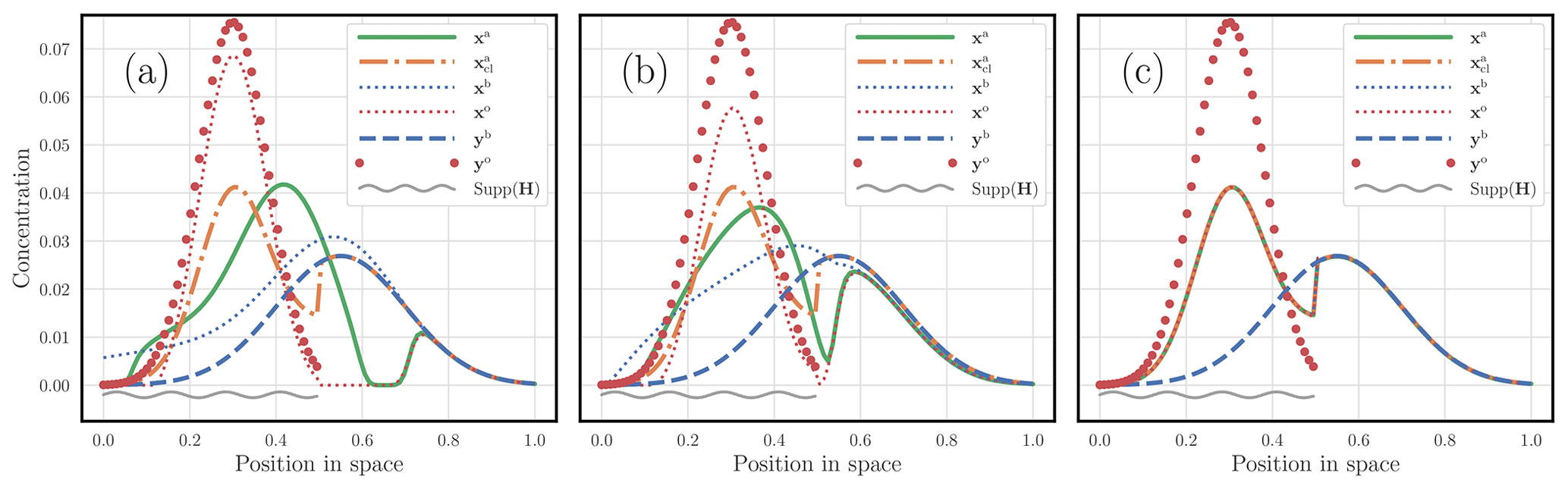
Figure 4a considers the DA problem based on Eq. (7), assuming that only half of the domain is observed. We have solved the corresponding mathematical and numerical problem as raised by Feyeux (2016) and displayed its solution. However, one observes that the mass of the solution concentrates on the observed subdomain and neglects the rest of the domain where the prior mainly concentrates, an outcome suspected by Feyeux (2016). Instead, we would have intuitively preferred a solution close to the one offered by Fig. 4b, whose formulation and numerical solution differ and follow the new approach developed in the present paper (how we obtained this solution will be described in Sect. 2).

Figure 4 The panels illustrate the analysis of a 3D-Var case that relies on the Wasserstein distance rather than a local metric. The red dots represent the observations, while the dashed blue curve represents the background state. The observations are only focused on the left half of the domain. The solution of the optimisation problem in Eq. (7) is displayed as a solid green curve in panel (a). The solution of the optimisation problem that we will propose in this paper is displayed as a solid green curve in panel (b). The support of the observation is suggested using a wavy grey segment. These states are typically one-dimensional puff pollutant concentrations. They should not be confused with pdfs of a single random variable.
The main caveat of Eq. (7) comes from the fact that the system is only partially observed, as well as the requirement that OT is balanced; i.e. the origin and target densities must have the same mass. This mass balance applies to both OT terms in Eq. (7), between yb and xa and between yo and Hxa:
Here, the mass of a vector x∈ℝN is defined by
with 1∈ℝN hereafter defined as the vector of entries 1.
Now, if we further assume, for simplicity, that yb and yo have the same mass (which is the case in Fig. 4), then
As a result, we obtain m(Hxa)=m(xa), which is an undesired prior piece of information as to where to find the mass of xa. Simply put, unless the system is fully observed, this approach amounts to the streetlight effect. This is precisely what happens in Fig. 4a with the undesired concentration of the mass of xa close to the edge of the observed subdomain.
To overcome this caveat and find a proper alternative to Eq. (7), we need (i) to renounce comparing the fields in observation space (in the observation discrepancy term of the cost function) and (ii) to introduce unbalanced OT (i.e. we need to be able to accommodate states of distinct masses). In the computer science context of pure OT, the latter has been discussed by Chizat et al. (2018). However, our solution differs formally and will be DA-centric.
1.6 Objective and outline
The objective of this paper is to lift the objection of Feyeux (2016) and propose a DA framework based on the Wasserstein distance, thereby offering a consistent way to bridge OT and classical DA. The new formalism will be referred to as hybrid OTDA (hybrid optimal transport data assimilation) in the rest of this paper (or OTDA for brevity). We will focus on the definition of a 3D-Var DA problem and how to obtain its analysis state and the associated analysis error covariance matrix.
At least within the perimeter of this paper, some restrictions apply. Firstly, the physical fields considered in the DA problem are non-negative (concentration of tracer, pollutants, water vapour, hydrometeors, chemical and biogeochemical species, etc.). However, as opposed to Feyeux (2016), the methods of this paper do not require the (possibly noisy) background state yb and observation yo to be non-negative. We stress once again that the states of our DA problem are physical fields onto which OT is applied and are not meant to be a pdf of a random variable. Secondly, the observation operator H is assumed to be linear. This is only meant for convenience and to obtain a rigorous correspondence between the primal and dual cost functions of the 3D-Var case. Making this assumption is very common in geophysical DA: H can indeed be seen as the tangent linear of a nonlinear observation operator within the inner loop of a 3D-Var or a 4D-Var case (see, for instance, Courtier, 1997).
The outline of the paper is as follows. After the present introduction (Sect. 1), Sect. 2 discloses our main idea and discusses two mathematical paths to solve the underlying optimisation problem; the first path is enlightening but not necessarily practical, whereas the alternative path is direct and robust but hides some of the concepts behind it. Section 3 provides one- and two-dimensional illustrations of a 3D-Var analysis based on the new hybrid OTDA formalism. These illustrations will show the possibilities and flexibility of the new framework. Importantly, Sect. 3 will also depict classical DA as a limit case of the formalism. In Sect. 4, the second-order analysis, i.e. the uncertainty quantification of the OTDA 3D-Var case, is derived, discussed, and illustrated. Conclusions and perspectives are given in Sect. 5.
2.1 Notation and conventions
Non-negative vectors x of size N are called discrete measures; they lie in the orthant . Although most mathematical OT theories work on normalised discrete measures, yielding probability vectors, this assumption will not be needed in this paper. The open subset of of all the positive discrete measures will be denoted as .
We will distinguish the observations and from the observable states and . yb, which corresponds to the first guess of conventional DA, and yo, which corresponds to the traditional observation vector, are known before solving the 3D-Var problem. These vectors embody all of the information processed in the analysis. By contrast, the observables xb and xo, which are related to yb and yo, respectively, through an observation operator (the identity for yb and xb), are not known a priori. They will be estimated along with the analysis state . Note that these vectors may well lie in distinct vector spaces of different dimensions; hence, the introduction of as many dimensions , and 𝒩o. can be seen as the value taken by x⋆ at site , for , and a and . Mind that the distinction between yb and xb and the introduction of xo are novelties of OTDA compared with classical DA.
Like in classical DA, the vectors yb and yo are subject to (prior) errors whose statistics are specified by the likelihoods p(yb|xb) and p(yo|xo), respectively. Up to constants that do not depend on , and yo, we assume the existence of ζb and ζo, such that
Thus, various error statistics can be considered. These errors are hypothesised to be mutually independent. The observation operator used in the definition of ζo is assumed to be linear. This qualification is for convenience and could be lifted if necessary. It is further assumed that ζb and ζo are strictly convex functions. This is, for instance, the case if we choose Gaussian error statistics yielding
Here, . B is the positive definite background error covariance matrix and R is the positive definite observation error covariance matrix. Finally, in the following, the m(⋆) operator will act not only on vectors but also, more generally, on any tensor, and it will return the sum of all of its entries.
2.2 Formalism of discrete optimal transport
To discretise and solve the continuous Kantorovich optimisation problem introduced in Sect. 1.3, we will need two elementary pieces of information about OT. These are not the only techniques that we will leverage, but both represent cornerstones towards a numerical solution to our proposal and, hence, require a proper introduction.
2.2.1 The primal cost function
Let us consider two discrete measures and with the same mass:
For convenience, will be used as an alias for the set . A cost matrix is given. The optimisation problem will be formulated using discrete Kantorovich transference plans . The optimal discrete transference plan is given by the minimiser of the following optimisation problem:
Here, the trace sums up the costs attached to each path, and the set of admissible transference plans is defined by
which selects the discrete transference plans with the proper marginals. could be viewed as a discrete equivalent to the square of the Wasserstein distance introduced in Eq. (5).
2.2.2 Entropic regularisation
The optimisation problem in Eq. (14) is a linear program that is convex (Peyré and Cuturi, 2019, and references therein). However, it is not generally strictly convex and, hence, does not necessarily exhibit a single minimum. Adding to the difficulty, its cost function (Eq. 14a) is constrained. Entropic regularisation addresses these issues and is used here to lift the constraints and to render the problem strictly convex. In particular, it will force any state vector that is a solution of the problem to be positive. A comprehensive justification is given by Peyré and Cuturi (2019). More precisely, we will use a Kullback–Leibler divergence (KL) regularisation term that is inserted in Eq. (14a),
which incorporates some prior transference plan νbo and does not require m(Pbo)=1, whereas Peyré and Cuturi (2019) opted for a basic entropy term. The KL term (Boyd and Vandenberghe, 2004) is defined by
It can be checked that the Hessian of the regularised cost function (Eq. 15) is a diagonal matrix of coefficients because , making the problem ε-strongly convex. We choose, for example, and ε>0, the latter of which is the regularisation scalar parameter. Note that this particular νbo is an admissible transference plan, i.e. it belongs to 𝒰bo, and can be interpreted as a complete statistical decoupling of the transference plan with respect to the origin and target discrete measures. In the limit of vanishing regularisation, the solution should not depend on the choice of νbo. However, the convergence to the solution at finite ε may depend on this choice. The primal cost function augmented with such an entropic regularisation is usually solved numerically with the iterative Sinkhorn algorithm (Sinkhorn, 1964). However, this is not the path followed in this paper, although we have used it as well.
Finally note that the technique to convexify such an optimisation problem with a KL term has been introduced in DA by Bocquet (2009) and Bocquet et al. (2011) following principles of statistical physics.
2.3 From classical data assimilation to hybrid optimal transport data assimilation
Figure 5 is a schematic representation of the flow of information in a classical DA update (and in particular 3D-Var), using the notation introduced above. In this case, the observables xb and xo and the analysis state xa are the same by construction; hence, xb and xo are not needed. This diagram, which could also be seen as a Bayesian network, corresponds to the cost function
to be minimised over xa. Now let us make use of the observables xb and xo as new degrees of freedom but bind them by OTs to xa, using the cost matrices Cba and Coa, respectively.
This yields the diagram in Fig. 6, which corresponds to the cost function
It must be minimised over xa, yielding an analysis state xa; this analysis state can also be seen as the W-barycentre between xb and xo. Note that xb and xo are discrete measures of unknown mass. For the optimisation problem, they lie in and , respectively.
Figure 5 A diagrammatic representation of the classical 3D-Var update, with the observations yb (the first guess) and yo (the observation vector), the analysis state xa, and the observed analysis Hxa. A double-line arrow represents a deterministic map, whereas a single-line arrow represents a statistical binding between the origin and the target.
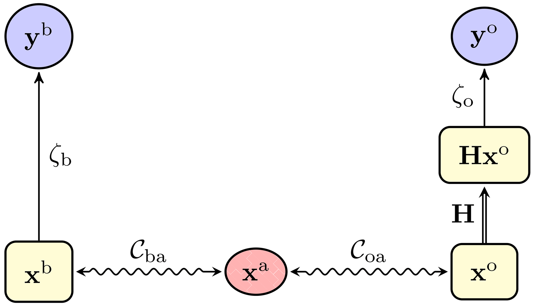
Figure 6 A diagrammatic representation of the hybrid OTDA 3D-Var update, with the observations yb (the first guess) and yo (the observation vector); the observables xb and xo; and xa, which is the W-barycentre. A double-line arrow represents a deterministic map, a single-line arrow represents a statistical binding between the origin and the target, and a wavy line represents the weaker bindings of xb with xa and xo with xa through OTs. This diagram can be seen as an unfolding of that in Fig. 5.
Moving from Eq. (17) to Eq. (18) following the principles and guidance of the introductory Sect. 1.4 is empirical, although no more than in Ning et al. (2014) and Feyeux (2016). Showing the merits of this move from Eq. (17) to Eq. (18) is the goal of the present paper. As opposed to Feyeux et al. (2018), it can deal with sparse and noisy observations, i.e. non-trivial H. We will show that classical DA is embedded in this generalisation. Moreover, the merits of the new cost function will be a posteriori qualitatively supported by the outcome of the numerical experiments (to the expert's eyes), which improve over previous formalism's outcomes. We would like to point out that we have also developed a consistent probabilistic and Bayesian formalism fully supporting the introduction of Eq. (18). However, we felt that the derivation was too long and technical for this paper and would not be helpful in the exploration of the direct consequences of Eq. (18).
We call Eq. (18) a high-level primal cost function because the metrics and have not yet been replaced by their transference plan expression, as opposed to, for example, Eq. (14a). Passing to a lower-level primal cost function would require expanding Eq. (18) using Eq. (14a) twice.
In the subsequent two subsections, we will investigate two pathways to solve the optimisation problem in Eq. (18). The first path (Sect. 2.4) unveils some of the key concepts behind its solution and partially disentangles the classical DA part from the W-barycentre part of the full analysis. This approach is enlightening but not necessarily practical. The second path is an alternative which is direct and robust but hides some of the fundamental principles underlying the solution. The busy reader could skip directly to the latter (i.e. Sect. 2.5).
2.4 Decomposition of the optimisation problem and effective cost metric
In this section, key ideas behind the minimisation of Eq. (18) are sketched and discussed. The level of mathematical rigour of this section is that of casual methodological DA in the geoscience literature. However, we stress that all of the algorithms discussed here have been successfully numerically tested on various configurations. The solution of Eq. (18) presented in this section is not necessarily robust, but it is enlightening and, hence, worth discussing.
Repeated contravariant indices – meaning the same tensor index is present as the upper and lower index – in tensor expressions will be understood as summed over, following Einstein's convention.
2.4.1 Dual formulation of the primal problem
One way, although not the only one, to write the explicit primal problem associated with Eq. (18) is through the use of a gluing transference plan , where (see pp. 11–12 of Vilani, 2009). is a 3-tensor whose marginals are xb, xo, and xa and that glues the transference plans Pba between xb and xa and Poa between xo and xa:
Here, the admissible set of (glued) transference plans, the set of all 3-tensors of non-negative entries whose marginals are xb, xo, and xa, is defined by
Due to the hardly scalable dimensionality of the primal problem, based on either a 3-tensor or a couple of 2-tensors, we wish to derive a dual problem equivalent to the primal one, using Lagrange multipliers to lift the constraints with (as will be checked later) a significantly smaller dimensionality.
This leads to a series of transformations of the problem ℒ, from a Lagrangian to a dual cost function, which is reported in Appendix A for the mathematically inclined reader. The outcome is a dual problem which reads
where the ∗ symbol refers to dual and where the polyhedron is defined by
In Eq. (20), the maps and are the Legendre–Fenchel transforms of the maps ζb and ζo, respectively. Let us recall that the Legendre–Fenchel transform of the map e↦ζ(e) is defined by . For instance, in the case of Gaussian error statistics (as in Eq. 12), these transforms are given by
Note that, in this section, we do not add the entropic regularisation to the cost functions for the sake of conciseness and because it does not play a role in the key ideas developed in this section; however, it would likely be added and employed in numerical applications.
2.4.2 Decomposition of the dual problem
These transformations allow us to trade the primal for the dual problem. Due to the fact that there are Na constraints indexed by for each fb and fo pair in and that the tightest of these constraints can account for the others, the problem in Eq. (20) should be equivalent to
where the polyhedron is defined by
and the effective cost metric Cbo is given (in the absence of entropic regularisation) by
According to Eq. (22c), this effective cost is given by the cost of the cheapest path(s), which is intuitive. The optimal transference glued plan, P, can be connected to the optimal transference plan Pbo between xb and xo with the cost Cbo in Eq. (22c), by marginalising on the intermediate density, i.e. the W-barycentre,
The solution for the analysis state xa is given by
by the definition of the marginals of the gluing transference plan P (Eq. 19c). However, we do not have direct access to the optimal gluing P from the dual problem (Eq. 22). This will be made simpler later on when adding the entropic regularisation to the problem.
For now, let us find an alternative solution bypassing the need for the gluing P and define the map
where 𝒫(S) is defined as the set of all subsets of S. The set lists all of the indices k that are relays to the transport in between the sites corresponding to index i and index j. That is why the W-barycentre can be obtained from Pbo:
In the next section, we will show how to estimate Pbo using entropic regularisation and, hence, leverage Eq. (26) to compute xa. κbo is reminiscent of the so-called McCann interpolant in OT theory, as it is only related to the OT between xb and xo, bypassing xa and, hence, the transference plan Pbo. Please refer to Remark 7.1 by Peyré and Cuturi (2019) and to Gangbo and McCann (1996) for a description of the McCann interpolant, even when there is no Monge map. This suggests that the analysis xa is not an interpolation of xb and xo in the space of values, as for classical DA, but along a geodesic in a Riemannian space built on a metric derived from the Wasserstein distance.
Nonetheless, the above derivation shows that we can trade a W-barycentre problem characterised by a couple of OT problems for a single OT problem defined by an effective metric Cbo. This principle is schematically illustrated in Fig. 7.
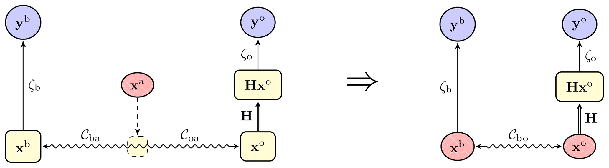
Figure 7 Trading a full hybrid OTDA problem, characterised by a W-barycentre defined by the cost metrics Cba and Coa, with a simplified hybrid OTDA problem, characterised by a single OT problem defined by an effective cost metric Cbo.
This suggests a simpler two-step algorithm, where the steps consist of the following: (i) solving a hybrid OTDA problem but with a single OT problem under an effective cost metric, which yields the analysed observables xb and xo, and (ii) computing the W-barycentre of xb and xo. To avoid making an overly large detour, the derivation of this algorithm is presented in Appendix B.
2.4.3 Classical data assimilation as a particular case
The primal problem (Eq. 17) of classical DA reads as follows:
Let us see how the OTDA formalism in Eq. (22) can account for classical DA. In the context of classical DA, the observable spaces for xb, xo, and xa are assumed to be the same by construction. Let us then define the cost matrices
i.e. it is assumed that the cost of moving masses is as large as it can be. Looking back at Eq. (19) but with these costs, it is clear that, in order to avoid the primal cost function being +∞, the transference plan Pijk must always be 0 unless . However, this implies, from the definition of 𝒰boa, that the observables coincide, , and that their mass is given by m(P). In this limit where the specific cost matrices are equal to and , the OTDA primal problem become mathematically equivalent to classical DA. Hence, classical DA is a limit case of OTDA. Note that, from its definition (Eq. 22c), the effective cost Cbo obtained from and coincides with .
2.5 A direct algorithmic solution
The two-step approach of Sect. 2.4 has merit in that it connects to the traditional W-barycentre problem, by first estimating xb and xo, and later computes the W-barycentre in between both states. It also suggests the existence of the effective cost metric of the problem. However, going through its consecutive steps may not be necessary for pure computational purposes. Here, we describe a direct approach that yields the analysis of the OTDA problem. It is less enlightening, but it is practical and will be used in the subsequent illustrations of the present paper.
An alternative formulation to the primal problem in Eq. (19) relies on two transference plans Pba and Poa corresponding to the two transports of the underlying W-barycentre problem, instead of the gluing one. Moreover, entropic regularisation is now enforced via 𝒦(Pba|νba) and 𝒦(Poa|νoa). The corresponding optimisation problem reads as follows:
where the admissible sets of the respective transference plans Pba and Poa are defined by
Following the same type of derivation as reported in the previous sections and Appendix B, the corresponding dual problem to be minimised is obtained as follows:
Here, discarding the constant , the associated regularised Lagrangian is
with a partition function associated with each transport:
where
It turns out that the optimal fa can be obtained analytically as a function of fb and fo, which we checked makes the optimisation numerically more efficient and robust. Indeed, let us introduce . We could optimise on ψ:
yielding the solution
Up to irrelevant constants, the resulting effective cost function using the optimal ψk is
Now, the optimal W-barycentre xa is given by either or , i.e.
from which we can infer the ψk-free expression
It is also useful to retrieve the optimal value of fa and obtain
so that we can compute the other two analysed observables, xb and xo, using
Note that most of these expressions can be assessed in a robust way in the log domain. For instance, in practice, we use, equivalently to Eqs. (35) and (37),
In this section, we showcase a selection of OTDA 3D-Var analyses. These are meant to stress the versatility of the formalism and the diverse solutions it offers, with significantly more degrees of freedom than in classical DA. The OTDA state analysis is carried out using the process in Sect. 2.5 and its formulas. Unless specifically discussed, entropic regularisation is used with . The dual cost function in Eq. (33) is minimised using the quasi-Newton method L-BFGS-B (Liu and Nocedal, 1989), which yields the optimal fb and fo. Then, Eq. (38) is employed to compute xb, xo, and xa.
3.1 One-dimensional examples
Considering the case in which the physical space of the fields is one-dimensional, we build bell-shaped observations yb and yo, related to an observable space of size shared by xb, xo, and xa. As yb is a fully observed instance of xb, we have , while 𝒩o may differ from No depending on the definition of the observation operator H. We choose (Gaussian statistics)
Here, . The states are discretised over the interval [0,1] at sites/grid cells for , with , and a. Unless otherwise specified, the cost metric has a quadratic dependence on the distance between sites, i.e. and . This is our reference set-up. The observation operator and the mass of the observations yb and yo will be specified for each experiment.
We consider four experiments in which we choose to vary key parameters in the OTDA set-up.
3.1.1 Varying the imbalance of the observation states
In the first experiment, the system is fully observed with H=I. We choose m(yb)=1 and the mass of yo to be in the set , with all the other parameters being fixed to the reference. The results are displayed in Fig. 8. Figure 8a corresponds to the case m(yo)=0.5. The resulting mass of the analysed observables is then . The adjustment of xb compared with yb and the adjustment of xo compared with yo, which are required to balance xb and xo, are patent. Figure 8b corresponds to the case m(yo)=1. The resulting mass of the analysed observables is then . No adjustment is required here because m(yo)=m(yb), and xo and yo as well as xb and yb coincide. Finally, the mass of yo is set to m(yo)=1.5 in Fig. 8c. The resulting mass of the analysed observables is then . The adjustment of xb compared with yb and the adjustment of xo compared with yo, which are required to balance xb and xo, are visually obvious, but the balancing goes in the opposite direction compared with Fig. 8a, as expected.
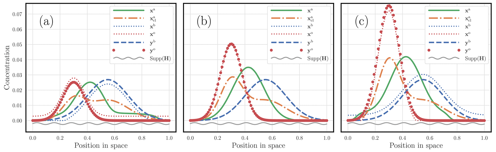
Figure 8 A hybrid OTDA 3D-Var analysis with one-dimensional physical states, where only the mass of yo is varied. Its mass is m(yo)=0.5 in panel (a), m(yo)=1 in panel (b), and m(yo)=1.5 in panel (c). The dashed blue curve corresponds to the first guess yb; the red dots correspond to the observations yo; the analysis state xa is the solid green curve; and the analysed observables xb and xo are blue and red dotted curves, respectively. The support of the observation is underlined by a wavy grey segment. The corresponding classical analysis is also plotted with a dot-dash orange curve. The x axis corresponds to the position in space; the y axis corresponds to the concentration value of the fields.
3.1.2 Varying the sparseness of the observation operator
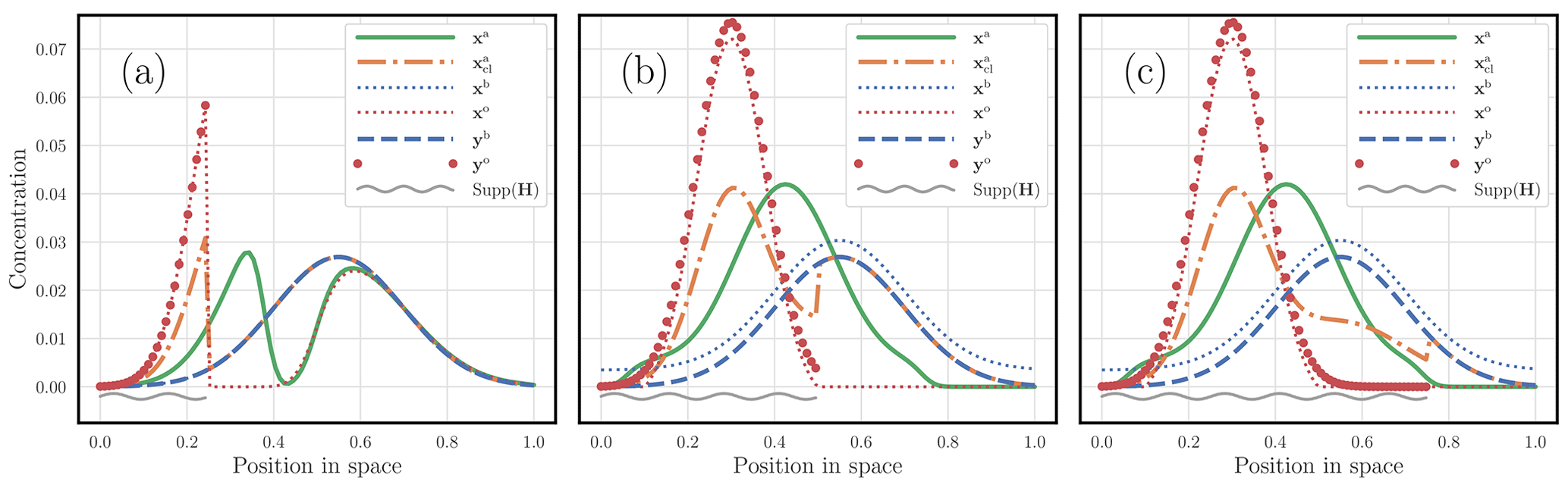
In this second experiment, with all of the other parameters being fixed to their reference value, only a fraction of the domain is observed, over , , and , where with , and for and .
The masses of the states that are built to generate yb and yo, before applying any observation operator, are set to 1 and 1.5, respectively. As a result, we have m(yb)=1, but m(yo) may depart from 1.5 depending on H. The fully observed case corresponds to Fig. 8c. The results are displayed in Fig. 9. It shows how smooth the OTDA solution can be compared with that of classical DA. However, as in Fig. 9a, OTDA can also handle obviously diverging sources of information, as is the case when the support of H is and when yo and yb can be seen to be barely consistent. In that case, the OTDA solution is smooth but bimodal.
3.1.3 Changing the nature of the cost metric
In this third experiment, we choose the cost metric to be of the form and . Only half of the domain is observed over , as in the case of Fig. 9b. As the mass of the state used to produce yo is 1.5, we have a slightly different m(yo)=1.49, with the rest of the mass being located in the unobserved part of the domain. All of the other parameters follow the reference set-up. The results are displayed in Fig. 10. For Fig. 10a, α is set to 0.5. For Fig. 10b, α is set to 1. For Fig. 10c, the cost metric is piecewise; it is quadratic, i.e. α=2, for pairs of sites separated by less than 10−1, i.e. , whereas the costs are chosen to be infinite for pairs of sites beyond this range. Hence, transport is prohibited beyond a distance of 10−1. The case of a pure quadratic cost corresponds to Fig. 9b. The impact on the shape of the OTDA analysis is very significant and suggests that one could easily tailor their own cost to suit their specific DA problem.

3.1.4 Classical data assimilation as a sub-case of the hybrid optimal transport data assimilation
In the fourth experiment, we would like to numerically check the theoretical prediction of Sect. 2.4.3. Consider again the reference configuration; however, only half of the domain, over , is observed, with and for and . Most importantly, the cost metric has a quadratic dependence on the distance between sites, i.e. and . The case λ=1 corresponds to Fig. 9b. Figure 11 shows the results corresponding to λ=103 for panel (a), λ=104 for panel (b), and λ=106 for panel (c). When λ is increased, the OTDA analysis should tend to the classical DA solution. This is indeed corroborated by Fig. 11 and supports the claim of Sect. 2.4.3. Note that, as opposed to the three earlier experiments, we had to tune ε here, as the wide range of λ has a significant impact on the balance of the key terms of the cost function (transport cost, discrepancy errors, and regularisation).
3.2 Two-dimensional examples
Considering the case in which the physical space of the fields is two-dimensional, we perform a couple of 3D-Var analyses on concentration fields (puffs of a pollutant). The states are discretised in the domain [0,1]2 at sites/grid cells for , with , and a. We choose , such that . Hence, the number of control variables is 3×10⁴. The observation vectors are yb and yo. As yb is a fully observed instance of xb, we have 𝒩b=Nb, while 𝒩o may differ from No depending on the definition of the observation operator H. Moreover, we choose (Gaussian statistics)
Here, . The entropic regularisation parameter is set to .
The first analysis is displayed in Fig. 12. The observation operator H is the identity, but its support is restricted to the subdomain [0,0.6]2. The plumes of pollutants yb and yo are generated from states formed as combinations of bell-like puffs. The system is unbalanced with m(yb)=1.35 and m(yo)=0.73. The cost metric has a quadratic dependence on the distance between sites, i.e. and . The OTDA analysis is clearly smoother than the classical solution. The classical solution does not cope very well with the seemingly disagreeing sources of information yb and yo, generating sharp transitions in the classical analysis. If yb and yo were consistently obtained from a truth perturbed with errors with short-range correlation, i.e. if they were drawn from the true prior distribution and in the absence of mislocation errors, then the classical analysis would be as good as it can be, whereas the OTDA solution may be too safe, i.e. too smooth. However, if one believes that structural errors and, in particular, location errors can impact yb and yo, then the classical solution is improper and the OTDA analysis preferable.
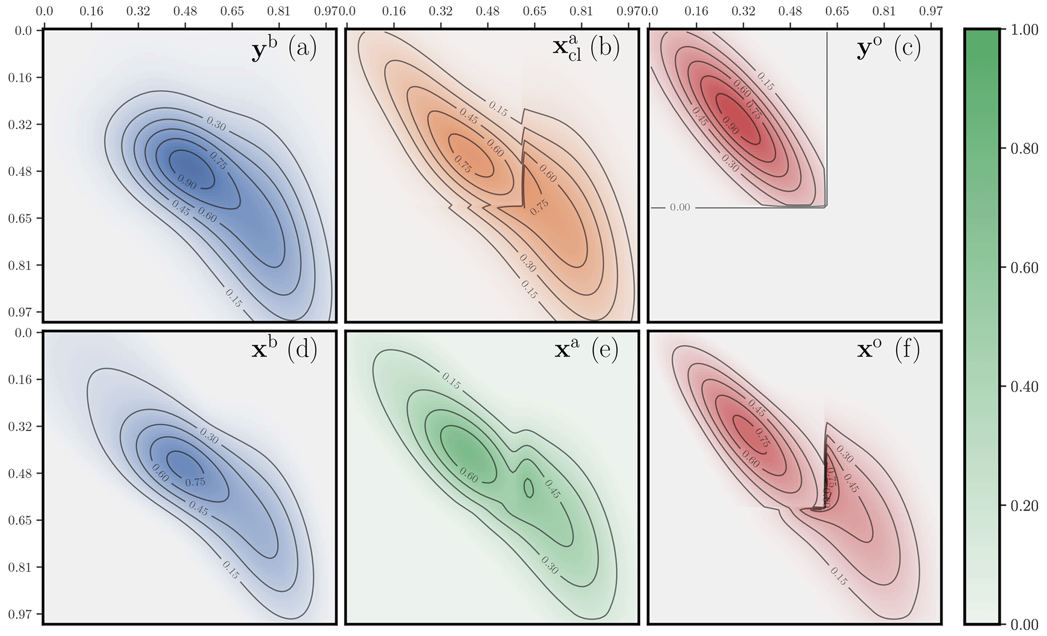
Figure 12 Two-dimensional concentration maps (plumes) of a hybrid OTDA analysis for the first configuration. The observations yb and yo; the analysed observables xb and xa, i.e. the state analysis; xo; and the corresponding classical DA analysis are displayed. All fields are rescaled so that their joint maximum is 1. All concentration maps use the same scale. The colour bar represents a unified contrast scale for the diverse field concentrations.
The second analysis is displayed in Fig. 13. The support of the observation operator H is again contained within the subdomain [0,0.6]2, but only one of four grid cells is actually observed in this area. The observation states yb and yo are generated from the same states as for Fig. 12. The system is unbalanced with m(yb)=1.35 and m(yo)=0.18. The cost metric is defined to be the same as in Fig. 12. The OTDA analysis is even smoother in this case compared with the classical DA analysis. It is much less impacted by the sparseness of the observation operator. The classical solution has to account for the staggered observations in the top left corner of the domain because the first guess in that region is very uncertain. By contrast, the OTDA solution assumes that location errors are possible; hence, it moves around the mass corresponding to these observations so that the structure of the observation operator is not as impactful on the analysis.
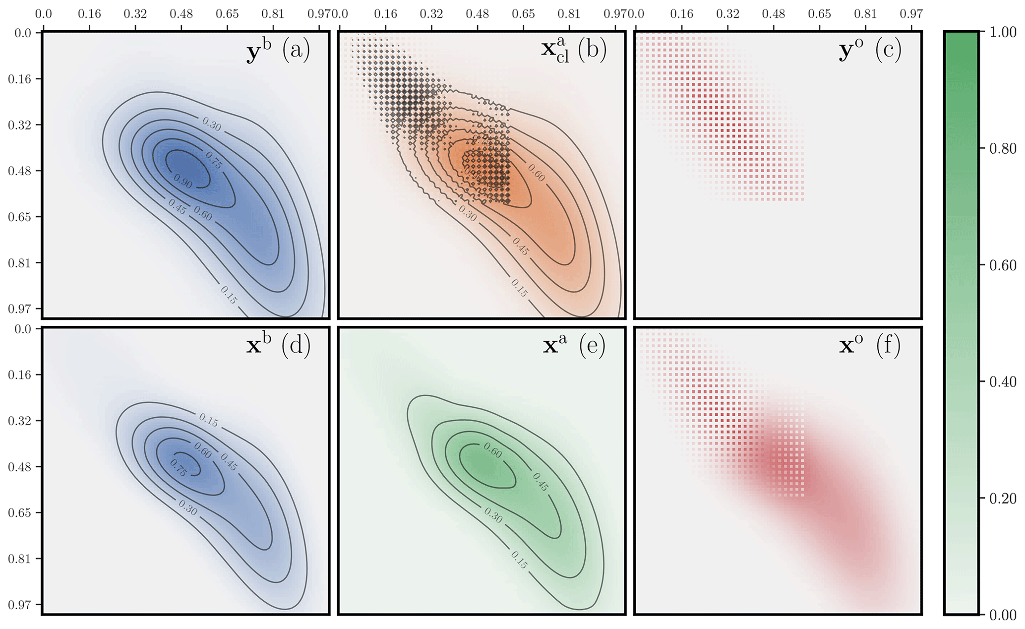
Figure 13 Two-dimensional concentrations maps of a hybrid OTDA analysis for the second configuration. The observations yb and yo; the analysed observables xb and xa, i.e. the state analysis; xo; and the corresponding classical DA analysis are displayed. Compared to Fig. 12, only H has changed. The level sets in panels (c) and (f) are omitted because they are driven by the staggered observation operator.
In this section, we compute the posterior error covariance matrix Pa associated with the state analysis xa, in order to complete the OTDA 3D-Var analysis description. There are many ways to proceed depending on the chosen regularisation and on the targeted degree of generality. Here, for the sake of consistency, we report on the way to derive Pa following the computation of the analysis state xa proposed in Sect. 2.5.
4.1 Mathematical results
Let us denote the compounded vectors of the observations, of the Lagrange multipliers, and of the observables as well as the compounded observation operator by
of size 𝒩b+𝒩o, 𝒩b+𝒩o, Nb+No, and , respectively. Similarly, we define the sum of the error statistics by , whose Legendre–Fenchel transform is . Using this notation, we can recapitulate the key results of Sect. 2.5: the effective dual cost function is
Here, the analysis state reads
where the dependence of the analysis state and the partition functions on f, fb, and fo is now emphasised and made explicit.
Any prior source of error in the system stems from the information vector y and hence drives the posterior error in the analysis xa. That is why we are interested in the sensitivity of xa with respect to y, i.e. . Denoting the expectation operator by 𝔼, the error covariance matrix is then defined by
from which a matrix factor Xa of Pa, i.e. which satisfies and whose expressions are usually much shorter than those of Pa, can be extracted, up to the multiplication by an orthogonal matrix on the right:
To compute the sensitivity matrix ∂yxa, we leverage the stationarity of the dual cost function at the minimum:
We resort to the implicit function theorem:
which yields
as , where Ibo is the identity matrix in the compounded observation space . The sensitivity ∂yxa can now be computed using the Leibniz chain rule and Eq. (48):
Let us now compute the Jacobian and Hessian in the right-hand side of Eq. (49). To that end and in order to externalise the observation operator, we introduce and , such that
and the related Jacobian and Hessians,
and can be shown to exist; they can be read off from the explicit expressions of Zε and xa as functions of f. These Jacobian and Hessians depend on the choice of the regularisation operator and need to be computed analytically, which is simple but tedious; this is not reported here, as it is a regularisation-dependent calculation. The Hessian of the dual cost function Eq. (42a) can then be written as the sum
while the sensitivity matrix now reads
Note that Ωbo,bo can be interpreted as the covariance matrix of x, the compounded observable vector as defined in Eq. (41) (although seen as a random vector), under the assumption that xb and xo are connected via the W-barycentre xa and the optimal transference plans Pba and Poa (all seen as random vectors). Combining Eqs. (52) and (53) with Eq. (45), we finally obtain the expression for a factor Xa of Pa:
Alternatively, we can use the Sherman–Morrison–Woodbury transformation, under the assumption that Ωbo,bo is invertible:
These formulas are similar to the normal equations of classical DA. However, it should be noted that, in Eqs. (54) and (55), all of the prior error statistics are encapsulated in Λbo,bo, whereas the impact of OT is encoded in Ωbo,bo. To be concrete, note that, when using Gaussian statistics (Eq. 12), Λbo,bo would simply read
4.2 Interpretation
Further, we can perform a block decomposition of Ω onto the spaces of xb and xo:
It can be shown that Ωbo is proportional to the optimal transference plan of the effective transport between xo and xb and that the blocks of the diagonal are themselves diagonal and depend on the observable states:
For instance, this could be shown by the explicit computation of .
Let us now examine the impact of OT on the analysis error covariance matrix. We first define
whose thin singular value decomposition is UΣV⊤, where U is an orthogonal matrix of size , Σ is a rectangular and diagonal matrix of size , and V is an orthogonal matrix of size . Then, we standardise Eq. (54) following, for example, Sect. 2.4.1 in Rodgers (2000):
Defining , which is a square diagonal of size , we obtain, up to a multiplication by an irrelevant orthogonal matrix on the right, an equivalent factor for Pa:
The diagonal values of σ, denoted σi≥0, represent the independent degrees of freedom (dof) values of information that can be extracted from the observations, which, in our case, is the first guess yb and the traditional observations yo, in contrast to Rodgers (2000), who only considers the dof values from yo. The higher the σi, the more information attached to the dof of index i and the more squeezed the corresponding direction in Xa and Pa. From Eq. (59) and, in particular, its transpose, , we can trace the flow of any piece of information. Such information stems from the observation vectors; hence, its flow starts in Δ⊤ from , the square root of the precision matrix . It is then transferred from the observation spaces to the observable spaces through 𝓗⊤. It is finally optimally transported across the space of xb and xo by Ωbo,bo, whose off-diagonal block is proportional to the transference plan Pbo. Hence, OT is not a primary source of uncertainty, as yb and yo can be, but moves information in between the observable spaces.
Let us now check the OTDA analysis error covariance matrix Pa in the classical DA limit. To that end, we study Eq. (54) in the classical limit. Similarly to Ωbb and Ωoo in Eq. (58a), Ωaa is defined as the covariance matrix of xa when only accounting for both OTs, and it can be shown that it reads
When the cost tends to , following the same arguments as in Sect. 2.4.3, xb, xo, and xa must merge and, consequently, . Hence, in this limit, and , with . Then, substituting these expressions of Ωbo,bo and Ωbo,a into Eq. (54), we get
Here, Ia is the identity matrix of size Na. From Eq. (62b) to Eq. (62c), we relied on the shift matrix lemma (e.g. Asch et al., 2016). For in Eq. (62d) to exist, it must be assumed that ; i.e. all the entries of xa are positive. This is verified when using entropic regularisation with ε>0, no matter how small the entries of xa are. Moreover, if xa has zero entries, xa can be represented as the limit of a sequence of positive discrete measures.
Now, as we have
we conclude, from Eq. (62d), that the classical limit of the analysis error covariance matrix is
If the limit of xa when is in , then must vanish. In this case,
which, assuming Gaussian errors, would read , as expected from classical DA. However, if some of the entries of xa vanish in the limit , we suspect that the limit of Pa will be the classical analysis error covariance matrix A but with the columns and rows associated with the vanishing entries of xa tapered to 0.
4.3 Numerical illustration
We consider the one-dimensional example where half of the domain is observed, over . Here, with and for and . Further, the observations are unbalanced, m(yb)=1 and m(yo)=1.49; they have been generated through 𝓗 by discrete measures of mass 1 and 1.5, respectively. Moreover, the cost metric has a quadratic dependence on the distance between sites, i.e. and , where λ=103. We use the results of Sect. 4.1 to compute the analysis error covariance matrix Pa, the transference plan Pbo, and the Jacobian Ωbo,a. The numerical results are displayed in Fig. 14. The OTDA analysis state is bimodal, with some mass being left over to the right of the domain to account for the long tail of the first guess, which is far from the observation support. Hence, there is a vanishing field region, roughly [0.6,0.7], which separates the two components of the analysis state. As expected from OT theory, Pbo seems to converge towards a (non-trivial and barely differentiable) Monge map which, in this discrete context, has two branches, separated by the gap created by the vanishing field region. The analysis error covariance matrix Pa seems to converge to a diagonal matrix, with the exception of the vanishing field region. Indeed, there seems to be an uncertainty with respect to how much mass should be transferred from the first guess tail [0.7,1] to the main region [0,0.6]. This is given away by variance peaks near the edges of the gap and by negative covariances between the two edge points of the gap.
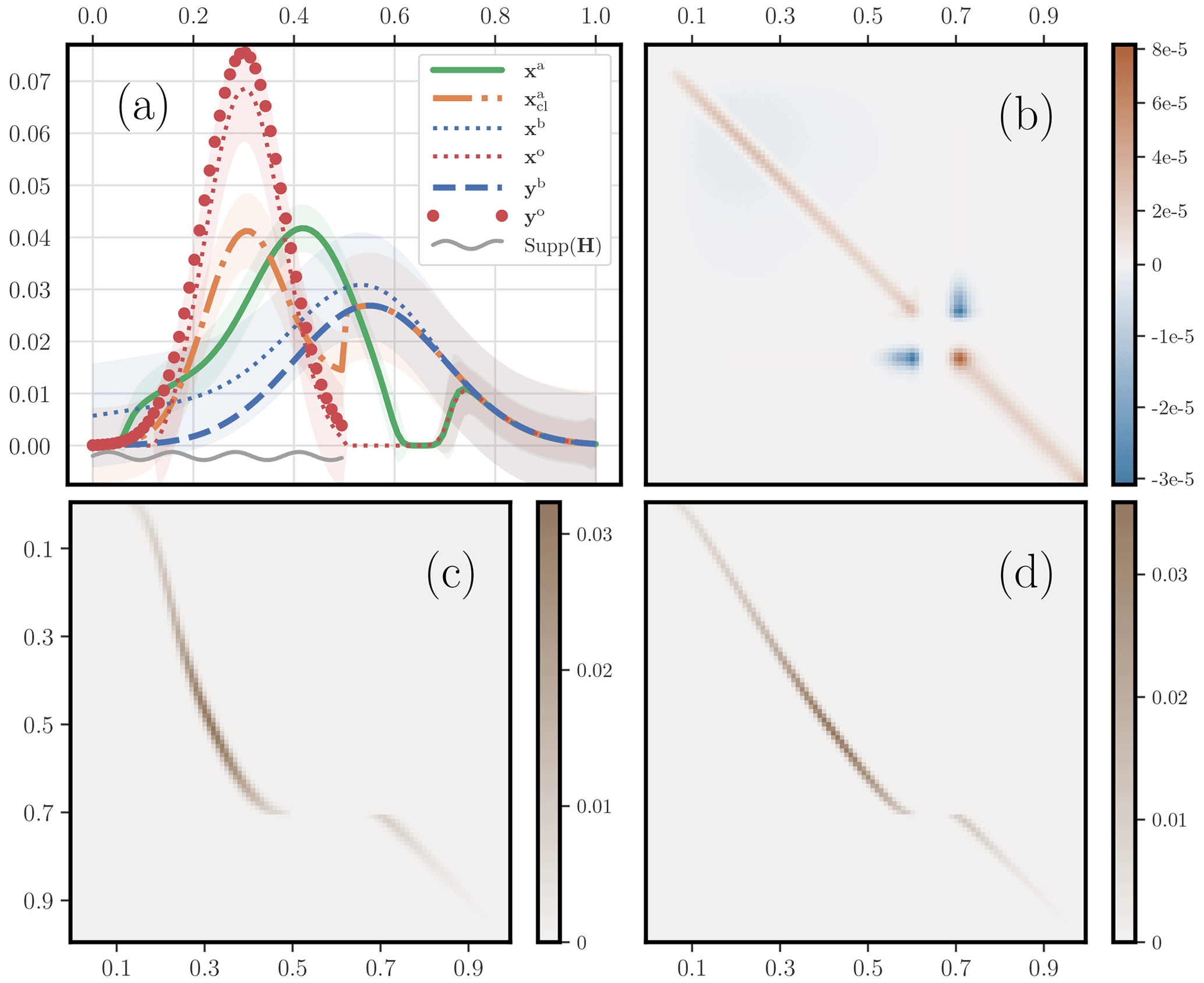
Figure 14 Illustration of the second-order analysis of an OTDA 3D-Var. Panel (a) shows the same plot as Fig. 11a but with the addition of shaded regions delineated by plus and minus the standard deviations about the estimates for , and xo. These standard deviations are computed from the diagonal of the diagnosed posterior error covariance matrices associated with xa, , xb, and xo. Panel (b) displays the analysis error covariance matrix Pa. Panel (c) shows the optimal transference plan Pbo. Panel (d) shows the a,b block part of the Jacobian matrix Ωbo,a, which is denoted Ωba.
In this paper, we have introduced a theoretical framework for integrating nonlocal optimal transport (OT) metrics into data assimilation (DA), which we refer to as hybrid OTDA. This framework addresses the inconsistencies initially identified by Feyeux et al. (2016) when local metrics in classical DA are replaced with nonlocal ones based on OT.
Our focus has been on defining a 3D-Var approach for hybrid OTDA and deriving the first- and second-order moments of its analysis. The hybrid OTDA 3D-Var method blends classical DA and its background and observation error statistics with a Wasserstein barycentre problem involving the observables associated with the first guess and the observation vector. Importantly, our work demonstrates that classical DA is encompassed within this theoretical framework.
We have shown that this optimisation problem can be decomposed and simplified into a hybrid OTDA problem with a single OT problem based on an effective cost. This first problem yields the estimated xb and xo, followed by a pure W-barycentre problem involving these states, whose solution is known as the McCann interpolant. This W-barycentre computation serves as the final analysis step.
Our proposed method can be applied to sparsely and noisily observed systems, as expected from a robust DA method. It can also accommodate non-trivial error statistics typical of a 3D-Var approach. Furthermore, we have illustrated the method's flexibility in defining cost metrics through various one- and two-dimensional numerical examples. We have empirically checked how the OTDA analysis shifts towards the classical DA analysis, within the OTDA framework. Note that, for now, some limitations apply; mainly, the framework is presently meant for non-negative fields.
While we have looked into several other promising developments regarding our methodology, we have chosen not to report them in this paper. These developments will be the subject of a future publication and include the following:
-
the derivation of a Bayesian and probabilistic standpoint on OTDA;
-
a generalised formalism enforcing physical regularisation, such as smoothness of the field, on the analysis state;
-
a stochastic matrix formalism, which is a substitute to using transference plans but could offer more robustness in the presence of entropic regularisation;
-
employing cost matrices defined across several spaces, which is useful for realistic application where xb and xo lie in very distinct spaces, such as the space of emission of a pollutant and the space of the pollutant concentrations, respectively.
While our primary focus in this paper was on the derivation and understanding of key cost functions within the hybrid OTDA framework, we did not delve much into the numerical challenges, algorithmic complexity, or computing acceleration. For this aspect of the developments, we would rather rely on developments from OT experts, who are continuously improving the efficiency of numerical OT (e.g. Flamary et al., 2021).
In addition to strengthening the developments mentioned above, our future research will explore the application of the hybrid OTDA formalism in a sequential DA framework, as this paper concentrated solely on static analysis. We are also interested in investigating the role played by error statistics and cost metrics and their balancing in the hybrid OTDA analysis as well as in developing their objective tuning.
This appendix is dedicated to the derivation of the transformation from a Lagrangian variant of the primal problem to the dual cost function (Eq. 20). It takes the form of the following series of transformations of the problem (from a Lagrangian to a dual cost function):
In Eq. (A1a), the maps and are the Legendre–Fenchel transforms of the maps ζb and ζo, respectively. From Eq. (A1d) to Eq. (A1eA1e), taking the minimum over the observables xb, xo, and xa implies enforcing hb=fb, , and fa=0. Hence, we obtain the dual problem which only depends on the Lagrange multipliers:
where the ∗ symbol refers to dual and where the polyhedron is defined by
The inequality constraints of the polyhedron stem from the positivity constraint Pijk≥0 in Eq. (A1eA1e). Very importantly, we have the coincidence of the minimum of the primal problem with the maximum of the dual problem , a property called strong duality (see Sect. 5.2 in Boyd and Vandenberghe, 2004). Strong duality can, for instance, be achieved if both the primal and dual cost functions are convex, which is the case here.
Here, we derive the two-step algorithm elaborated in Sect. 2.4.2. Moreover, entropic regularisation is added to the problem.
B1 First step: simplified hybrid optimal transport data assimilation problem
The first step of the full OTDA algorithm is a simplified OTDA problem based on a single OT problem driven by the cost Cbo. The corresponding high-level primal cost function is
The associated (lower-level) primal cost function, adding entropic regularisation (ε>0), is then
In this optimisation problem, the admissible set of transference plans, i.e. the set of all 2-tensors of non-negative entries whose marginals are xb and xo, is defined by
As xb and xo are not predetermined, the prior transference plan ν cannot be selected from 𝒰bo a priori. Hence, the simplest choice, which we decided to implement, is to set νij to a constant, which assumes some statistical prior independence of xb and xo. A derivation of the dual problem equivalent to ℒε can be obtained in the exact same way as in the previous subsection, although it is now less cluttered because there is only one OT to account for, instead of two. The associated Lagrangian is
Again, the maps and are the Legendre–Fenchel transforms of the maps ζb and ζo, respectively. The variables fb and fo are Lagrange vectors; they are used to enforce the marginals of the transference plan associated with . The unconstrained minimisation over P, i.e. the inner minimisation problem in Eq. (B3), is obtained by cancelling the gradient with respect to P, which yields
Substituting this solution into minus the Lagrangian −ℒε gives the regularised dual problem
with the associated Lagrangian
which relies on the partition function
The notation and , rather than and , signifies that we work on the opposite of and so as to obtain a dual problem to be minimised rather than maximised. Most importantly, we have, under conditions that will be satisfied in the following, the coincidence of the two minima , i.e. strong duality. Assuming one can obtain a proper correspondence between the optimal fb and fo of the dual problem and xb and xo of the primal problem, this implies, once again, that the primal problem can be traded for the dual problem.
Even though the regularised optimisation problem is slightly different from the unregularised one, a difference which is controlled by the value of ε, the new dual optimisation problem is free, i.e. without constraints. It can be solved as it is, using, for instance, the L-BFGS-B minimiser (Liu and Nocedal, 1989). The advantage of the regularised dual formulation is twofold: (1) the dual cost function is unconstrained (free optimisation), and (2) we will trade a minimisation over Nb×No variables for a minimisation over Nb+No variables. This dual formulation can be viewed as a generalised physical-space statistical analysis system (PSAS) formalism (Courtier, 1997), an approach in which classical DA algebra is mostly carried out in observation space.
Once the optimal values for fb and fo are obtained, the optimal discrete Kantorovich transference plan P can be computed using Eq. (B4). As a result, as marginals of this transference plan, the solutions for the observables are
B2 Second step: Wasserstein barycentre
Now that we have obtained the observables xb and xo via Eq. (B6), we would like to compute their W-barycentre. The joint mass m of these observables can be computed as follows:
The high-level primal cost function of this W-barycentre problem is
We have found and practised several ways to solve this problem. One way is to compute the McCann interpolant. This is theoretically elegant, but Eq. (26) did not leverage regularisation of the W-barycentre problem. Instead, the approach reported here is to use the dual optimisation problem, in conjunction with entropic regularisation at finite ε>0. We leverage our knowledge of the mass m resulting from the first step of the algorithm by enforcing the mass in the cost function, m(P)=m. This seems redundant, but it actually yields, by construction and very naturally, a numerically efficient algorithm comparable to the ad hoc log-domain scheme proposed in Sect. 4.4 of Peyré and Cuturi (2019).
Again, one way (although not the only way) to write the primal problem is to use a gluing transference plan, a 3-tensor whose marginals are xb, xo, and xa:
where , the binary operator ⋅ denotes the contraction of tensors, and
The 3-tensor ν is chosen to be , which is uniform in k and for which m(ν)=m. The resulting dual problem is
where the associated Lagrangian is
with the partition function
This partition function is elegant but impractical because, with high dimensionality, a 3-tensor might be too large to store and compute with. However the partition function in Eq. (B10c) can be simplified by noticing that
where we introduced the effective cost metric
which is the regularised cost – known in statistics and machine learning as a soft-plus transform – of Eq. (22c). The 2-tensor νij plays the same role as that of the first step of the algorithm; we choose it as , for which m(ν)=m. The dual problem now only involves 2-tensors and becomes numerically more efficient. Given the optimal fb and fo, the (glued) optimal transference plan Pboa is formally given by
The W-barycentre xa is then given as a marginal of Pboa:
Because of the normalisation of the transference plan to m, the entropic regularisation exhibits a εmln Zε instead of εZε. This systematically enforces normalisation in the computations of the gradients, as well as in the course of the numerical optimisation of the dual cost function, de facto working in the log domain. We experienced more stable computations and the ability to reach smaller ε, compared with the case without normalisation. This completes the solution through the two-step OTDA algorithm.
The products of this paper are exclusively optimisation problems and methods to solve them; their implementation (code) used in the illustrative sections relies on freely available software to solve the optimisation problems, mainly L-BFGS-B and its implementation in SciPy (https://github.com/scipy/scipy, SciPy, 2024) and the Python Optimal Transport library and its implementation (https://github.com/PythonOT, Optimal Transport, 2024).
No data sets were used in this article.
MB, PJV, and AF developed the methodology. MB implemented the numerics. MB wrote the manuscript. MB, PJV, AF, JDLB, and YR revised the manuscript.
The contact author has declared that none of the authors has any competing interests.
Publisher’s note: Copernicus Publications remains neutral with regard to jurisdictional claims made in the text, published maps, institutional affiliations, or any other geographical representation in this paper. While Copernicus Publications makes every effort to include appropriate place names, the final responsibility lies with the authors.
The authors would like to thank Oliver Talagrand (the executive and handling editor) and the two anonymous reviewers for their remarks and suggestions that helped shape the paper. This research has been supported by the ANR-ARGONAUT (PollutAnt and gReenhouse Gases emissiOns moNitoring from spAce at high ResolUTion) national research project (grant no. ANR-19-CE01-0007). CEREA is a member of Institut Pierre-Simon Laplace (IPSL).
This research has been supported by the Agence Nationale de la Recherche (grant no. ANR-19-CE01-0007).
This paper was edited by Olivier Talagrand and reviewed by two anonymous referees.
Amodei, M. and Stein, J.: Deterministic and fuzzy verification methods for a hierarchy of numerical models, Meteorol. Appl., 16, 191–203, https://doi.org/10.1002/met.101, 2009. a, b
Asch, M., Bocquet, M., and Nodet, M.: Data Assimilation: Methods, Algorithms, and Applications, Fundamentals of Algorithms, SIAM, Philadelphia, ISBN 978-1-611974-53-9, https://doi.org/10.1137/1.9781611974546, 2016. a, b
Bocquet, M.: Towards optimal choices of control space representation for geophysical data assimilation, Mon. Weather Rev., 137, 2331–2348, https://doi.org/10.1175/2009MWR2789.1, 2009. a
Bocquet, M., Wu, L., and Chevallier, F.: Bayesian design of control space for optimal assimilation of observations. I: Consistent multiscale formalism, Q. J. Roy. Meteor. Soc., 137, 1340–1356, https://doi.org/10.1002/qj.837, 2011. a
Boyd, S. P. and Vandenberghe, L.: Convex optimization, Cambridge university press, ISBN 978-0521833783, 2004. a, b
Briggs, W. M. and Levine, R. A.: Wavelets and field forecast verification, Mon. Weather Rev., 125, 1329–1341, https://doi.org/1520-0493(1997)125<1329:WAFFV>2.0.CO;2, 1997. a
Carrassi, A., Bocquet, M., Bertino, L., and Evensen, G.: Data Assimilation in the Geosciences: An overview on methods, issues, and perspectives, WIREs Clim. Change, 9, e535, https://doi.org/10.1002/wcc.535, 2018. a
Chizat, L., Peyré, G., Schmitzer, B., and Vialard, F.-X.: Scaling algorithms for unbalanced optimal transport problems, Math. Comput., 87, 2563–2609, https://doi.org/10.1090/mcom/3303, 2018. a
Courtier, P.: Dual formulation of four-dimensional variational assimilation, Q. J. Roy. Meteor. Soc., 123, 2449–2461, https://doi.org/10.1002/qj.49712354414, 1997. a, b
Daley, R.: Atmospheric Data Analysis, Cambridge University Press, New-York, ISBN 9780521458252, 1991. a
Davis, C., Brown, B., and Bullock, R.: Object-based verification of precipitation forecasts. Part I: Methodology and application to mesoscale rain areas, Mon. Weather Rev., 134, 772–1784, https://doi.org/10.1175/MWR3146.1, 2006a. a
Davis, C., Brown, B., and Bullock, R.: Object-based verification of precipitation forecasts. Part II: Application to convective rain systems, Mon. Weather Rev., 134, 1785–1795, https://doi.org/10.1175/MWR3145.1, 2006b. a
Duc, L. and Sawada, Y.: Geometry of rainfall ensemble means: from arithmetic averages to Gaussian-Hellinger barycenters in unbalanced optimal transport, J. Meteor. Soc. Jpn., 102, 35–47, https://doi.org/10.2151/jmsj.2024-003, 2024. a
Ebert, E. E.: Fuzzy verification of high-resolution gridded forecasts: a review and proposed framework, Meteorol. Appl., 15, 51–64, https://doi.org/10.1002/met.25, 2008. a
El Moselhy, T. A. and Marzouk, Y. M.: Bayesian inference with optimal maps, J. Comp. Phys., 231, 7815–7850, https://doi.org/10.1016/j.jcp.2012.07.022, 2012. a
Evensen, G., Vossepoel, F. C., and van Leeuwen. P. J.: Data Assimilation Fundamentals: A Unified Formulation of the State and Parameter Estimation Problem, Springer Textbooks in Earth Sciences, Geography and Environment, Springer Cham, ISBN 978-3-030-96708-6, https://doi.org/10.1007/978-3-030-96709-3, 2022. a
Farchi, A. and Bocquet, M.: Review article: Comparison of local particle filters and new implementations, Nonlin. Processes Geophys., 25, 765–807, https://doi.org/10.5194/npg-25-765-2018, 2018. a
Farchi, A., Bocquet, M., Roustan, Y., Mathieu, A., and Quérel, A.: Using the Wasserstein distance to compare fields of pollutants: application to the radionuclide atmospheric dispersion of the Fukushima-Daiichi accident, Tellus B, 68, 31682, https://doi.org/10.3402/tellusb.v68.31682, 2016. a, b
Feyeux, N.: Transport optimal pour l'assimilation de données images, Ph.D. thesis, Université Grenoble Alpes, https://inria.hal.science/tel-01480695 (last access: 7 July 2024), 2016. a, b, c, d, e, f, g, h, i
Feyeux, N., Vidard, A., and Nodet, M.: Optimal transport for variational data assimilation, Nonlin. Processes Geophys., 25, 55–66, https://doi.org/10.5194/npg-25-55-2018, 2018. a, b, c, d, e
Flamary, R., Courty, N., Gramfort, A., Alaya, M. Z., Boisbunon, A., Chambon, S., Chapel, L., Corenflos, A., K., F., Fournier, N., Gautheron, L., Gayraud, N. T. H., Janati, H., Rakotomamonjy, A., Redko, I., Rolet, A., Schutz, A., Seguy, V., Sutherland, D. J., Tavenard, R., Tong, A., and Vayer, T.: POT: Python Optimal Transport, J. Mach. Learn. Res., 22, 1–8, http://jmlr.org/papers/v22/20-451.html (last access: 7 July 2024), 2021. a
Gangbo, W. and McCann, R. J.: The geometry of optimal transportation, Acta Math., 177, 113–1618, https://doi.org/10.1007/BF02392620, 1996. a
Gilleland, E., Ahijevych, D. A., Brown, B. G., and Ebert, E. E.: Verifying forecasts spatially, B. Am. Meteorol. Soc., 91, 1365–1373, https://doi.org/10.1175/2010BAMS2819.1, 2010a. a
Gilleland, E., Lindström, J., and Lindgren, F.: Analyzing the image warp forecast verification method on precipitation fields from the ICP, Weather Forecast., 25, 1249–1262, https://doi.org/10.1175/2010WAF2222365.1, 2010b. a
Hoffman, R. N. and Grassotti, C.: A Technique for Assimilating SSM/I Observations of Marine Atmospheric Storms: Tests with ECMWF Analyses, J. Appl. Meteorol. Clim., 35, 1177–1188, https://doi.org/10.1175/1520-0450(1996)035<1177:ATFASO>2.0.CO;2, 1996. a
Hoffman, R. N., Liu, Z., Louis, J.-F., and Grassoti, C.: Distortion representation of forecast errors, Mon. Weather Rev., 123, 2758–2770, https://doi.org/10.1175/1520-0493(1995)123<2758:DROFE>2.0.CO;2, 1995. a, b
Janjić, T., Bormann, N., Bocquet, M., Carton, J. A., Cohn, S. E., Dance, S. L., Losa, S. N., Nichols, N. K., Potthast, R., Waller, J. A., and Weston, P.: On the representation error in data assimilation, Q. J. Roy. Meteor. Soc., 144, 1257–1278, https://doi.org/10.1002/qj.3130, 2018. a
Kalnay, E.: Atmospheric Modeling, Data Assimilation and Predictability, Cambridge University Press, Cambridge, ISBN 9780521796293, 2003. a
Keil, C. and Craig, G. C.: A displacement and amplitude score employing an optical flow technique, Weather Forecast., 24, 1297–1308, https://doi.org/10.1175/2009WAF2222247.1, 2009. a
Lack, S. A., Limpert, G. L., and Fox, N. I.: An object-oriented multiscale verification scheme, Weather Forecast., 25, 79–92, https://doi.org/10.1175/2009WAF2222245.1, 2010. a
Le Coz, C., Tantet, A., Flamary, R., and Plougonven, R.: Optimal transport for the multi-model combination of sub-seasonal ensemble forecasts, EGU General Assembly 2023, Vienna, Austria, 24–28 Apr 2023, EGU23-13445, https://doi.org/10.5194/egusphere-egu23-13445, 2023. a
Liu, D. C. and Nocedal, J.: On the limited memory BFGS method for large scale optimization, Math. Programm., 45, 503–528, https://doi.org/10.1007/BF01589116, 1989. a, b
Lledó, L., Skok, G., and Haiden, T.: Estimating location errors in precipitation forecasts with the Wasserstein and Attribution distances, EMS Annual Meeting 2023, Bratislava, Slovakia, 4–8 Sep 2023, EMS2023-602, https://doi.org/10.5194/ems2023-602, 2023. a
Marzouk, Y., Moselhy, T., Parno, M., and Spantini, A.: An introduction to sampling via measure transport, in: Handbook of Uncertainty Quantification, edited by: Ghanem, R., Higdon, D., and Owhadi, H., chap. 23, Springer International Publishing, Cham, 785–825, https://doi.org/10.1007/978-3-319-12385-1_23, 2017. a
Monge, G.: Mémoire sur la théorie des déblais et des remblais, in: Histoire de l'Académie Royale des Sciences de Paris, 666–704, 1781. a
Necker, T., Wolfgruber, L., Kugler, L., Weissmann, M., Dorninger, M., and Serafin, S.: The fractions skill score for ensemble forecast verification, Authorea [preprint], https://doi.org/10.22541/au.169169008.89657659/v1, 2023. a
Ning, L.and Carli, F. P., Ebtehaj, A. M., Foufoula-Georgiou, E., and Georgiou, T. T.: Coping with model error in variational data assimilation using optimal mass transport, Water Resour. Res., 50, 5817–5830, https://doi.org/10.1002/2013WR014966, 2014. a, b
Oliver, D. S.: Minimization for conditional simulation: Relationship to optimal transport, J. Comp. Phys., 265, 1–15, https://doi.org/10.1016/j.jcp.2014.01.048, 2014. a
Optimal Transport: Github [code], https://github.com/PythonOT, last access: 7 July 2024. a
Peyré, G. and Cuturi, M.: Computational Optimal Transport: With Applications to Data Science, Foundations and Trends in Machine Learning, 11, 355–607, https://doi.org/10.1561/2200000073, 2019. a, b, c, d, e, f, g, h
Plu, M.: A variational formulation for translation and assimilation of coherent structures, Nonlin. Processes Geophys., 20, 793–801, https://doi.org/10.5194/npg-20-793-2013, 2013. a
Ravela, S., Emanuel, K., and McLaughlin, D.: Data assimilation by field alignement, Physica D, 230, 127–145, https://doi.org/10.1016/j.physd.2006.09.035, 2007. a
Rodgers, C. D.: Inverse methods for atmospheric sounding, vol. 2, World Scientific, Series on Atmospheric, Oceanic and Planetary Physics, ISBN 978-981-02-2740-1, https://doi.org/10.1142/3171, 2000. a, b
SciPy: SciPy library main repository, Github [code], https://github.com/scipy/scipy, last access: 7 July 2024. a
Sinkhorn, R.: A relationship between arbitrary positive matrices and doubly stochastic matrices, Ann. Math. Stat., 35, 876–879, 1964. a
Skok, G.: Precipitation attribution distance, Atmos. Res., 295, 106998, https://doi.org/10.1016/j.atmosres.2023.106998, 2023. a
Talagrand, O.: Assimilation of Observations, an Introduction, J. Meteor. Soc. Jpn., 75, 191–209, https://doi.org/10.2151/jmsj1965.75.1B_191, 1997. a
Tamang, S. K., Ebtehaj, A., Zou, D., and Lerman, G.: Regularized variational data assimilation for bias treatment using the W asserstein metric, Q. J. Roy. Meteor. Soc., 146, 2332–2346, https://doi.org/10.1002/qj.3794, 2020. a
Tamang, S. K., Ebtehaj, A., van Leeuwen, P. J., Zou, D., and Lerman, G.: Ensemble Riemannian data assimilation over the Wasserstein space, Nonlin. Processes Geophys., 28, 295–309, https://doi.org/10.5194/npg-28-295-2021, 2021. a
Tamang, S. K., Ebtehaj, A., van Leeuwen, P. J., Lerman, G., and Foufoula-Georgiou, E.: Ensemble Riemannian data assimilation: towards large-scale dynamical systems, Nonlin. Processes Geophys., 29, 77–92, https://doi.org/10.5194/npg-29-77-2022, 2022. a
Vanderbecken, P. J., Dumont Le Brazidec, J., Farchi, A., Bocquet, M., Roustan, Y., Potier, É., and Broquet, G.: Accounting for meteorological biases in simulated plumes using smarter metrics, Atmos. Meas. Tech., 16, 1745–1766, https://doi.org/10.5194/amt-16-1745-2023, 2023. a, b
Vilani, C.: Topics in Optimal Transportation, vol. 58 of Graduate Studies in Mathematics, American Mathematical Society, Providence, Rhode Island, ISBN 9780821833124, 2003. a
Vilani, C.: Optimal Transport: Old and New, vol. 338 of Die Grundlehren der Mathematischen Wissenschaften, Springer-Verlag, Berlin Heidelberg, ISBN 978-3-540-71049-3, 2009. a, b
Wernli, H., Paulat, M., Hagen, M., and Frei, C.: SAL – A Novel Quality Measure for the Verification of Quantitative Precipitation Forecasts, Mon. Weather Rev., 136, 4470–4487, https://doi.org/10.1175/2008MWR2415.1, 2008. a, b
Ying, Y.: A Multiscale Alignment Method for Ensemble Filtering with Displacement Errors, Mon. Weather Rev., 147, 4553–4565, https://doi.org/10.1175/MWR-D-19-0170.1, 2019. a
Ying, Y., Anderson, J. L., and Bertino, L.: Improving Vortex Position Accuracy with a New Multiscale Alignment Ensemble Filter, Mon. Weather Rev., 151, 1387–405, https://doi.org/10.1175/MWR-D-22-0140.1, 2023. a
Zhou, W., Bovik, A. C., Sheikh, H. R., and Simoncelli, E.: Image quality assessment: from error visibility to structural similarity, IEEE T. Image Process., 13, 600–612, https://doi.org/10.1109/TIP.2003.819861, 2004. a
- Abstract
- Introduction
- The main proposal
- Numerical illustrations
- Uncertainty quantification
- Conclusions
- Appendix A: From the primal to the dual cost function for the full problem
- Appendix B: Derivation of the two-step hybrid optimal transport data assimilation algorithm
- Code availability
- Data availability
- Author contributions
- Competing interests
- Disclaimer
- Acknowledgements
- Financial support
- Review statement
- References