Leading the Lorenz 63 system toward the prescribed regime by model predictive control coupled with data assimilation

Recently, concerns have been growing about the intensification and increase in extreme weather events, including torrential rainfall and typhoons. For mitigating the damage caused by weather-induced disasters, recent studies have started developing weather control technologies to lead the weather to a desirable direction with feasible manipulations. This study proposes introducing the model predictive control (MPC), an advanced control method explored in control engineering, into the framework of the control simulation experiment (CSE). In contrast to previous CSE studies, the proposed method explicitly considers physical constraints, such as the maximum allowable manipulations, within the cost function of the MPC. As the first step toward applying the MPC to real weather control, this study performed a series of MPC experiments with the Lorenz 63 model. Our results showed that the Lorenz 63 system can be led to the positive regime with control inputs determined by the MPC. Furthermore, the MPC significantly reduced necessary forecast length compared to earlier CSE studies. It was beneficial to select a member that showed a larger regime shift for the initial state when dealing with uncertainty in initial states.

1 Introduction

In recent years, concerns have been raised regarding the intensification and increase in extreme weather events such as torrential rainfall and typhoons. To mitigate the damage caused by weather-induced disasters, efforts have been made to improve the forecasting accuracy of stationary heavy rainfall and develop disaster prevention infrastructures, including dams and embankments. Recently, Japan's Moonshot program started exploring alternative countermeasures for mitigating weather-induced disasters. Specifically, the program aims at developing weather control technologies to lead the weather to a desirable regime with feasible manipulations. Under the program, researchers are exploring various engineering techniques such as cloud seeding and atmospheric heating. However, the possible magnitude of humans' manipulations of the atmosphere is limited. Therefore, simulation studies using numerical weather prediction (NWP) models are needed in addition to the engineering studies to develop effective control approaches with feasible manipulations.

To date, a few simulation studies with NWP models have been conducted for mitigating extreme events. For example, Henderson et al. (2005) conducted numerical experiments using a modified version of the Fifth-Generation Penn State/NCAR Mesoscale Model (MM5) 4D-Var to identify the temperature increments required for minimizing wind-related damage caused by Hurricane Andrew in 1992. However, the results may not be sufficiently realistic due to various experimental limitations (Henderson et al., 2005). The Typhoon Science and Technology Research Center of Yokohama National University proposed using sailing ships and artificial upwelling to reduce the intensity of tropical cyclones. Their simulations demonstrated that the drag enhancement caused by the sailing ships and sea surface temperature decrease by the artificial upwelling successfully weakened tropical cyclones (Hironori Fudeyasu; personal communication, 2023). Previous studies, however, examined impacts of the manipulations on specific extreme events through control experiments that simply compared simulations with and without manipulations. Here, a research framework is necessary to develop effective control approaches with feasible manipulations.

Miyoshi and Sun (2022; hereafter MS22) proposed a control simulation experiment (CSE), an experimental framework for systematically evaluating and exploring control approaches with unknown true values by expanding the observing systems simulation experiment (OSSE). They conducted CSEs with the three-variable Lorenz 63 model (Lorenz, 1963) and succeeded in leading the system to the positive regime with small control inputs. Sun et al. (2023; hereafter SMR23) also applied to CSEs for the 40-variable Lorenz 96 model (Lorenz, 1996), showing that their CSEs succeeded in reducing the number of extreme events of the Lorenz 96 model. Furthermore, Ouyang et al. (2023; hereafter OTK23) successfully reduced the total magnitude of control inputs with the Lorenz 63 model by approximately 20 % compared to MS22's approach by regulating the amplitude of control inputs based on the maximum growth rate of the singular vector. The previous CSE studies (MS22, SMR23, and OTK23) generated control inputs as differences between ensemble members that stay within and those that deviate from the desired regime. However, physical constraints, generally needed for real-world applications, cannot be explicitly considered in previous CSE studies. Therefore, it is worthwhile to explore other methodologies to determine control inputs.

In this study, we propose introducing the model predictive control (MPC) within the framework of CSE. The MPC is an advanced control method that repeats prediction and optimization with explicit consideration of constraints. While the MPC has been widely used in practical fields such as the process industry and power electronics (Schwenzer et al., 2021), there has been no study yet that used the MPC for mitigating weather-induced disasters to the best of our knowledge. As the first step toward applying the MPC to the real weather control, this study performs a series of MPC experiments with the Lorenz 63 model. Here we explore the way to implement the MPC within CSE and aim to reveal important issues to extend the MPC to high-dimensional NWP models.

The remaining sections of this paper are arranged as follows. Section 2 introduces the theory of the MPC and describes the experimental setting. In Sect. 3, we employ a series of MPC experiments with the Lorenz 63 model and discuss properties of the MPC applied to the chaotic dynamical systems. Finally, Sect. 4 provides a summary.

2 Method and experiments

2.1 Model predictive control

2.1.1 Definition and procedure

This study explores using the MPC for controlling a chaotic dynamical system. Here, the MPC is a feedback control method that identifies control inputs to minimize the cost function under constraints at each time. In other words, the MPC is a control method that solves an optimal control problem (OCP) for a finite horizon at each time. Strictly speaking, the MPC considered in this study is nonlinear model predictive control (Chen and Shaw, 1982; Keerthi and Gilbert, 1988; Mayne and Michalska, 1990; Mayne et al., 2000).

First, we define the terminology and symbols. As shown in Fig. 1, the two key processes of the MPC are model-based prediction and optimization of control inputs in the OCP. For these processes, the prediction horizon, T_p, and the control horizon, T_c, are defined independently, where subscripts p and c denote prediction and control. Here, T_p (0<T_p) is the length of state prediction and T_c ($\mathrm{0}<T_{\mathrm{c}}\le T_{\mathrm{p}}$) is the length of the control inputs to be optimized. A new axis, τ, is the time axis for variables under the optimization and set to be different from the time axis, t. Therefore, τ=0 denotes the initial times of the horizons. Furthermore, variables in both horizons are marked with a superscript ∗; for example, a state x at τ=τ_i on the horizon at t=t_i is denoted by ${\mathit{x}}^{\ast }\left({\mathit{\tau }}_i;t_i\right)$.

Next, we describe the procedure of the MPC. First, the MPC requires the suitable design of a numerical model, $f\left({\mathit{x}}^{\ast },{\mathit{u}}^{\ast }\right)$; a cost function, $J\left({\mathit{x}}^{\ast },{\mathit{u}}^{\ast }\right)$; a set of constraints, $\mathit{c}\left({\mathit{x}}^{\ast },{\mathit{u}}^{\ast }\right)$; and a first guess of control inputs, ${\mathit{u}}^{\ast }\left(\mathit{\tau };t_i\right)$, from τ=0 to τ=T_c for the desirable control. Now, we consider the process of obtaining the control input, u, at t=t_i based on the MPC.

1. The present state x(t_i) is used as the initial state ${\mathit{x}}^{\ast }\left(\mathrm{0};t_i\right)$ for an OCP (i.e., ${\mathit{x}}^{\ast }\left(\mathrm{0};t_i\right)=\mathit{x}\left(t_i\right)$).

2. The predicted state, ${\mathit{x}}^{\ast }\left(\mathit{\tau };t_i\right)$, from τ=0 to τ=T_p is obtained by the numerical model, $f\left({\mathit{x}}^{\ast },{\mathit{u}}^{\ast }\right)$.

3. Based on ${\mathit{x}}^{\ast }\left(\mathit{\tau };t_i\right)$, the solution ${\mathit{u}}^{\ast }\left(\mathit{\tau };t_i\right)$ is updated from τ=0 to τ=T_c through optimization (see Sect. 2.1.2).

4. Prediction (step 2) and optimization (step 3) are iterated with updated ${\mathit{u}}^{\ast }\left(\mathit{\tau };t_i\right)$ and ${\mathit{x}}^{\ast }\left(\mathrm{0};t_i\right)$ until ${\mathit{u}}^{\ast }\left(\mathit{\tau };t_i\right)$ is sufficiently converged (see Sect. 2.1.2).

5. The control input, u(t), taken from finally updated ${\mathit{u}}^{\ast }\left(\mathit{\tau };t_i\right)$ from τ=0 to $\mathit{\tau }=k\cdot \mathrm{d}t$ ($\mathrm{0}<k\cdot \mathrm{d}t<T_{\mathrm{c}}$), is used for the manipulation from t=t_i to $t=t_i+k\cdot \mathrm{d}t$.

6. The process returns to step 1 and repeats these steps at $t=t_i+k\cdot \mathrm{d}t$.

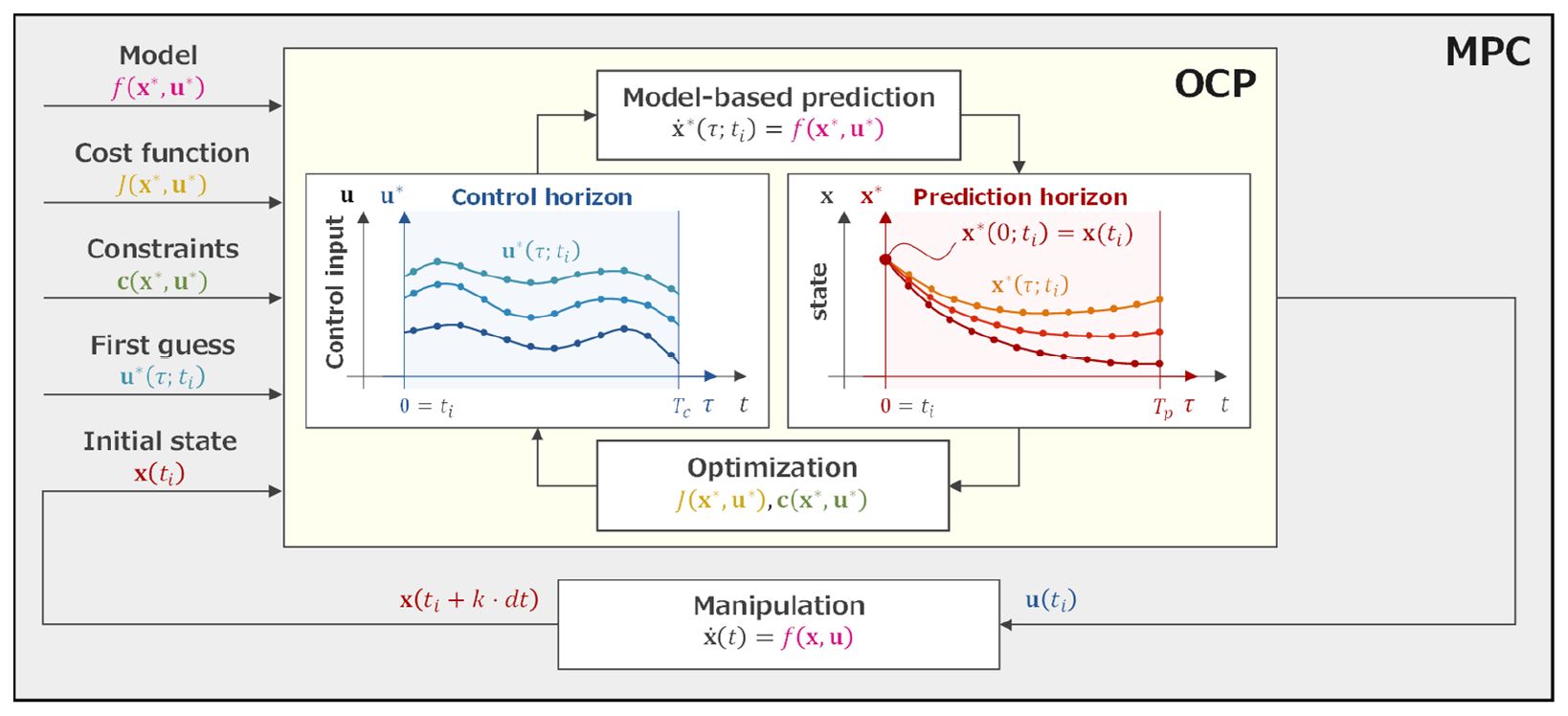
Figure 1 Conceptual image of the model predictive control (MPC; the gray block). A numerical model, $f\left({\mathit{x}}^{\ast },{\mathit{u}}^{\ast }\right)$; a cost function, $J\left({\mathit{x}}^{\ast },{\mathit{u}}^{\ast }\right)$; a set of constraints, $\mathit{c}\left({\mathit{x}}^{\ast },{\mathit{u}}^{\ast }\right)$; and a first guess of control inputs, ${\mathit{u}}^{\ast }\left(\mathit{\tau };t_i\right)$, are given to the optimal control problem (OCP; the yellow block). The initial state, x(t_i), is also given by the model time integration with manipulations. The OCP is solved by iterating prediction and optimization until the solution u(t_i) is sufficiently converged. Finally, the manipulation is performed by applying the u(t_i) to x(t_i). The same process is repeated at the next time ($t=t_i+k\cdot \mathrm{d}t$).

2.1.2 Optimal control problem

As previously noted, the MPC identifies control inputs that allow the system to achieve a desirable state for a finite horizon by solving the OCP at each time. Here, we explain that the OCP can be regarded as a variational problem with constraints. We consider a basic OCP with control and prediction horizons being $T=T_{\mathrm{c}}=T_{\mathrm{p}}$ for ease of comprehension. The general equations of state for a nonlinear model and the initial state are given by

$$\begin{array}{}\text{(1)}& {\displaystyle }{\dot{\mathit{x}}}^{\ast }\left(\mathit{\tau };t\right)=f\left({\mathit{x}}^{\ast }\left(\mathit{\tau };t\right),{\mathit{u}}^{\ast }\left(\mathit{\tau };t\right)\right),\text{(2)}& {\displaystyle }{\mathit{x}}^{\ast }\left(\mathrm{0};t\right)=\mathit{x}\left(t\right),\end{array}$$

where their dimensions are ${\mathit{x}}^{\ast }\left(\mathit{\tau };t\right)\in R^n$ and ${\mathit{u}}^{\ast }\left(\mathit{\tau };t\right)\in R^l$, respectively. The scalars n and l represent the number of model variables and manipulation variables, respectively. The general cost function of the OCP is given by

$$\begin{array}{}\text{(3)}& J\left({\mathit{x}}^{\ast },{\mathit{u}}^{\ast }\right)=\mathit{\phi }\left({\mathit{x}}^{\ast }\left(T;t\right)\right)+\underset{\mathrm{0}}{\overset{T}{\int }}L\left({\mathit{x}}^{\ast }\left(\mathit{\tau };t\right),{\mathit{u}}^{\ast }\left(\mathit{\tau };t\right)\right)\mathrm{d}\mathit{\tau },\end{array}$$

where $\mathit{\phi }\left({\mathit{x}}^{\ast }\left(T;t\right)\right)$ is the terminal cost and $L\left({\mathit{x}}^{\ast }\left(\mathit{\tau };t\right),{\mathit{u}}^{\ast }\left(\mathit{\tau };t\right)\right)$ is the stage cost. Both are scalar functions, and various control objectives can be considered by a suitable design of these functions. The general constraints of the problem are given by

$$\begin{array}{}\text{(4)}& \mathit{c}\left({\mathit{x}}^{\ast }\left(\mathit{\tau };t\right),{\mathit{u}}^{\ast }\left(\mathit{\tau };t\right)\right)=\left[\begin{array}{c}{c}_{\mathrm{1}}\left({\mathit{x}}^{\ast }\left(\mathit{\tau };t\right),{\mathit{u}}^{\ast }\left(\mathit{\tau };t\right)\right)\\ \mathrm{⋮}\\ c_j\left({\mathit{x}}^{\ast }\left(\mathit{\tau };t\right),{\mathit{u}}^{\ast }\left(\mathit{\tau };t\right)\right)\end{array}\right]=\mathit{0},\end{array}$$

where $\mathit{c}\left({\mathit{x}}^{\ast }\left(\mathit{\tau };t\right),{\mathit{u}}^{\ast }\left(\mathit{\tau };t\right)\right)\in R^j$ is a vector whose elements are equality constraints restricted to zero. The scalar j is the number of constraints. When inequality constraints are imposed, the constrained problem can be addressed by methods such as the penalty method or the slack variable technique. This study uses the penalty method, which adds large penalties to the cost function when the constraints are not satisfied (see Eq. 26). On the other hand, the slack variable technique converts inequality constraints to equality constraints by introducing dummy variables. The addition of the dummy variables, however, makes the OCP more complicated. Therefore, we did not use the slack variable technique in this study. In summary, the OCP is regarded as the following variational problem that optimizes the cost function, subject to the equation of state and constraints:

$$\begin{array}{}\text{(5)}& {\displaystyle }\begin{array}{rl}\mathrm{minimize}J\left({\mathit{x}}^{\ast },{\mathit{u}}^{\ast }\right)& =\mathit{\phi }\left({\mathit{x}}^{\ast }\left(T;t\right)\right)\\ & +\underset{\mathrm{0}}{\overset{T}{\int }}L\left({\mathit{x}}^{\ast }\left(\mathit{\tau };t\right),{\mathit{u}}^{\ast }\left(\mathit{\tau };t\right)\right)\mathrm{d}\mathit{\tau }\end{array},\text{(6)}& {\displaystyle }\mathrm{subject}\mathrm{to}\left\{\begin{array}{l}f\left({\mathit{x}}^{\ast }\left(\mathit{\tau };t\right),{\mathit{u}}^{\ast }\left(\mathit{\tau };t\right)\right)-{\dot{\mathit{x}}}^{\ast }\left(\mathit{\tau };t\right)=\mathit{0},\\ {\mathit{x}}^{\ast }\left(\mathrm{0};t\right)=\mathit{x}\left(t\right),\\ \mathit{c}\left({\mathit{x}}^{\ast }\left(\mathit{\tau };t\right),{\mathit{u}}^{\ast }\left(\mathit{\tau };t\right)\right)=\mathit{0}.\end{array}.\right.\end{array}$$

We note that the equation of state (Eq. 1) is also regarded as an equality constraint (the first equation in Eq. 6) by transposing ${\dot{\mathit{x}}}^{\ast }\left(\mathit{\tau };t\right)$ of Eq. (1) to the right-hand side.

The following necessary conditions for optimal control inputs are obtained by converting the constrained problem to an unconstrained problem using the method of Lagrange multipliers (see Appendix A):

$$\begin{array}{}\text{(7)}& {\displaystyle }{\dot{\mathit{x}}}^{\ast }\left(\mathit{\tau };t\right)=f\left({\mathit{x}}^{\ast }\left(\mathit{\tau };t\right),{\mathit{u}}^{\ast }\left(\mathit{\tau };t\right)\right),\text{(8)}& {\displaystyle }{\mathit{x}}^{\ast }\left(\mathrm{0};t\right)=\mathit{x}\left(t\right),\text{(9)}& {\displaystyle }{\dot{\mathit{\lambda }}}^{\ast }\left(\mathit{\tau };t\right)=-{\displaystyle \frac{\partial H\left({\mathit{x}}^{\ast },{\mathit{u}}^{\ast },{\mathit{\lambda }}^{\ast },{\mathit{\rho }}^{\ast }\right)}{\partial \mathit{x}}},\text{(10)}& {\displaystyle }{\mathit{\lambda }}^{\ast }\left(T;t\right)={\displaystyle \frac{\partial \mathit{\phi }\left({\mathit{x}}^{\ast }\left(T;t\right)\right)}{\partial \mathit{x}}},\text{(11)}& {\displaystyle \frac{\partial H\left({\mathit{x}}^{\ast },{\mathit{u}}^{\ast },{\mathit{\lambda }}^{\ast },{\mathit{\rho }}^{\ast }\right)}{\partial \mathit{u}}}=\mathit{0},\text{(12)}& {\displaystyle }\mathit{c}\left({\mathit{x}}^{\ast }\left(\mathit{\tau };t\right),{\mathit{u}}^{\ast }\left(\mathit{\tau };t\right)\right)=\mathit{0},\end{array}$$

where ${\mathit{\lambda }}^{\ast }\left(\mathit{\tau };t\right)\in R^n$ is the Lagrange multiplier for the equation of state, ${\mathit{\rho }}^{\ast }\left(\mathit{\tau };t\right)\in R^j$ is the Lagrange multiplier for the constraints, and $H\left({\mathit{x}}^{\ast },{\mathit{u}}^{\ast },{\mathit{\lambda }}^{\ast },{\mathit{\rho }}^{\ast }\right)$ is the Hamiltonian defined as

$$\begin{array}{}\text{(13)}& \begin{array}{rl}H\left({\mathit{x}}^{\ast },{\mathit{u}}^{\ast },{\mathit{\lambda }}^{\ast },{\mathit{\rho }}^{\ast }\right)& :=L\left({\mathit{x}}^{\ast },{\mathit{u}}^{\ast }\right)+{\left({\mathit{\lambda }}^{\ast }\right)}^{T}f\left({\mathit{x}}^{\ast },{\mathit{u}}^{\ast }\right)\\ & +{\left({\mathit{\rho }}^{\ast }\right)}^T\mathit{c}\left({\mathit{x}}^{\ast },{\mathit{u}}^{\ast }\right).\end{array}\end{array}$$

The derivation of the necessary conditions of the optimal control inputs is detailed in Appendix A. For nonlinear models, it is generally impossible to solve these equations analytically. Therefore, this study solves them using a numerical approach. Given the first guess of the control input, ${\mathit{u}}^{\ast }\left(\mathit{\tau };t\right)$, temporal forward computations (Eqs. 7 and 8) are performed to obtain ${\mathit{x}}^{\ast }\left(\mathit{\tau };t\right)$ from τ=0 to τ=T. In this study, zero vectors are selected as the first guess of the control input, ${\mathit{u}}^{\ast }\left(\mathit{\tau };t\right)$, because the minimization of the control input is also included in the cost function, $J\left({\mathit{x}}^{\ast },{\mathit{u}}^{\ast }\right)$, as seen later (Eq. 26). Furthermore, ${\mathit{\lambda }}^{\ast }\left(\mathit{\tau };t\right)$ is obtained by temporal backward computations from τ=T to τ=0 (Eqs. 9 and 10). Consequently, ${\mathit{u}}^{\ast }\left(\mathit{\tau };t\right)$ and ${\mathit{\rho }}^{\ast }\left(\mathit{\tau };t\right)$ from τ=0 to τ=T can be obtained by applying an optimization algorithm to the nonlinear equations (Eqs. 11 and 12). Therefore, the OCP can be solved by iterating the prediction (Eq. 7) and optimization (Eqs. 11 and 12) until the solutions are sufficiently converged. In this study, the equations (Eqs. 7–12) are discretized with the fourth-order Runge–Kutta scheme. In addition, we used the Levenberg–Marquardt algorithm, which is the optimization algorithm for solving the nonlinear equations (Eqs. 11 and 12). In our preliminary experiments, the Levenberg-Marquardt algorithm solved the nonlinear equations stably compared to other optimization methods in SciPy libraries.

When the control horizon is shorter than the prediction horizon (T_c<T_p), the necessary conditions for optimal control inputs (Eqs. 7–12) are replaced by

$$\begin{array}{}\text{(14)}& {\displaystyle }{\dot{\mathit{x}}}^{\ast }\left(\mathit{\tau };t\right)=\left\{\begin{array}{ll}{f}_{\mathrm{c}}\left({\mathit{x}}^{\ast }\left(\mathit{\tau };t\right),{\mathit{u}}^{\ast }\left(\mathit{\tau };t\right)\right)& \left(\mathrm{0}\le \mathit{\tau }<T_{\mathrm{c}}\right),\\ f_{\mathrm{p}}\left({\mathit{x}}^{\ast }\left(\mathit{\tau };t\right)\right)& \left(T_{\mathrm{c}}\le \mathit{\tau }<T_{\mathrm{p}}\right),\end{array}\right.\text{(15)}& {\displaystyle }{\mathit{x}}^{\ast }\left(\mathrm{0};t\right)=\mathit{x}\left(t\right),\text{(16)}& {\displaystyle }{\dot{\mathit{\lambda }}}^{\ast }\left(\mathit{\tau };t\right)=\left\{\begin{array}{ll}-\frac{\partial H_{\mathrm{c}}\left({\mathit{x}}^{\ast },{\mathit{u}}^{\ast },{\mathit{\lambda }}^{\ast },{\mathit{\rho }}^{\ast }\right)}{\partial \mathit{x}}& \left(\mathrm{0}\le \mathit{\tau }<T_{\mathrm{c}}\right),\\ -\frac{\partial H_{\mathrm{p}}\left({\mathit{x}}^{\ast },{\mathit{\lambda }}^{\ast },{\mathit{\rho }}^{\ast }\right)}{\partial \mathit{x}}& \left(T_{\mathrm{c}}\le \mathit{\tau }<T_{\mathrm{p}}\right),\end{array}\right.\text{(17)}& {\displaystyle }{\mathit{\lambda }}^{\ast }\left(T_{\mathrm{p}};t\right)={\displaystyle \frac{\partial \mathit{\phi }\left({\mathit{x}}^{\ast }\left(T_{\mathrm{p}};t\right)\right)}{\partial \mathit{x}}},\text{(18)}& {\displaystyle }\begin{array}{ll}\frac{\partial H_{\mathrm{c}}\left({\mathit{x}}^{\ast },{\mathit{u}}^{\ast },{\mathit{\lambda }}^{\ast },{\mathit{\rho }}^{\ast }\right)}{\partial \mathit{u}}=\mathit{0}& \left(\mathrm{0}\le \mathit{\tau }<T_{\mathrm{c}}\right),\end{array}\text{(19)}& {\displaystyle }\left\{\begin{array}{ll}{\mathit{c}}_{\mathrm{c}}\left({\mathit{x}}^{\ast }\left(\mathit{\tau };t\right),{\mathit{u}}^{\ast }\left(\mathit{\tau };t\right)\right)=\mathit{0}& \left(\mathrm{0}\le \mathit{\tau }<T_{\mathrm{c}}\right),\\ {\mathit{c}}_{\mathrm{p}}\left({\mathit{x}}^{\ast }\left(\mathit{\tau };t\right)\right)=\mathit{0}& \left(T_{\mathrm{c}}\le \mathit{\tau }<T_{\mathrm{p}}\right),\end{array}\right.\end{array}$$

where the subscript c denotes a function up to T_c with the control input, ${\mathit{u}}^{\ast }\left(\mathit{\tau };t\right)$, and the subscript p denotes the function from T_c to T_p without the control input.

2.2 Model predictive control for the Lorenz 63 model

2.2.1 The Lorenz 63 model

This study uses the Lorenz 63 model for MPC experiments. The Lorenz 63 model is a three-variable nonlinear differential equation expressed as follows:

$$\begin{array}{}\text{(20)}& {\displaystyle }\dot{x}=-\mathit{\sigma }x+\mathit{\sigma }y,\text{(21)}& {\displaystyle }\dot{y}=-xz+rx-y,\text{(22)}& {\displaystyle }\dot{z}=xy-bz.\end{array}$$

The model is known to behave in a chaotic manner under certain parameter values. In this study, σ=10, r=28, and $b=\mathrm{8}/\mathrm{3}$ are selected to form a butterfly pattern with two positive and negative regimes, following previous studies (MS22 and OTK23). Moreover, the model is discretized and integrated using the fourth-order Runge–Kutta scheme. One time step of integration is defined as dt=0.01 units of time throughout this study. With the Lorenz 63 model, the state vector becomes $\mathit{x}={\left[x,y,z\right]}^T$ and the number of model variable is n=3.

2.2.2 The optimal control problem with the Lorenz 63 model

This study considers a control problem, namely keeping the Lorenz 63 system in the positive regime (x≥0) following previous studies (MS22 and OTK23). Note that our approach includes minimization of the control inputs owing to Eq. (26). The equations of state (Eq. 14) are given by

$$\begin{array}{}\text{(23)}& {\displaystyle }{f}_{\mathrm{c}}\left({\mathit{x}}^{\ast },{\mathit{u}}^{\ast }\right)=\left[\begin{array}{c}-\mathit{\sigma }{x}^{\ast }+\mathit{\sigma }{y}^{\ast }+u_x^{\ast }\\ -x^{\ast }{z}^{\ast }+r{x}^{\ast }-y^{\ast }+u_y^{\ast }\\ x^{\ast }{y}^{\ast }-b{z}^{\ast }+u_z^{\ast }\end{array}\right],\text{(24)}& {\displaystyle }{f}_{\mathrm{p}}\left({\mathit{x}}^{\ast }\right)=\left[\begin{array}{c}-\mathit{\sigma }{x}^{\ast }+\mathit{\sigma }{y}^{\ast }\\ -x^{\ast }{z}^{\ast }+r{x}^{\ast }-y^{\ast }\\ x^{\ast }{y}^{\ast }-b{z}^{\ast }\end{array}\right],\end{array}$$

where ${\mathit{x}}^{\ast }={\left[x^{\ast },y^{\ast },z^{\ast }\right]}^T$ and ${\mathit{u}}^{\ast }={\left[u_x^{\ast },u_y^{\ast },u_z^{\ast }\right]}^T$. As previously noted, one of the control objectives in this problem is leading the Lorenz 63 system to the positive regime. Therefore, the inequality constraint, $x^{\ast }\left(\mathit{\tau };t\right)\ge \mathrm{0}$, is imposed from τ=0 to τ=T_p. In this study, the penalty method is introduced to treat the inequality constraint and the penalty function for $x^{\ast }\left(\mathit{\tau };t\right)\ge \mathrm{0}$ is defined as follows:

$$\begin{array}{}\text{(25)}& P_{x^{\ast }\ge \mathrm{0}}\left(x^{\ast }\right):={\displaystyle \frac{\mathrm{1}}{\mathrm{2}}}{\left\{\max \left(-x^{\ast },\mathrm{0}\right)\right\}}^{\mathrm{2}}.\end{array}$$

The inequality constraint can be considered in the cost function as follows. Including the minimization of the control inputs, the cost function is given by

$$\begin{array}{}\text{(26)}& \begin{array}{rl}J& =\underset{\mathrm{0}}{\overset{T_{\mathrm{c}}}{\int }}\left\{{\displaystyle \frac{\mathrm{1}}{\mathrm{2}}}{\left({\mathit{u}}^{\ast }\right)}^T{\mathit{u}}^{\ast }+{\mathit{\alpha }}_{x^{\ast }\ge \mathrm{0}}\cdot P_{x^{\ast }\ge \mathrm{0}}\left(x^{\ast }\right)\right\}\mathrm{d}\mathit{\tau }\\ & +\underset{T_{\mathrm{c}}}{\overset{T_{\mathrm{p}}}{\int }}{\mathit{\alpha }}_{x^{\ast }\ge \mathrm{0}}\cdot P_{x^{\ast }\ge \mathrm{0}}\left(x^{\ast }\right)\mathrm{d}\mathit{\tau }\\ & +{\mathit{\alpha }}_{x^{\ast }\ge \mathrm{0}}\cdot P_{x^{\ast }\ge \mathrm{0}}\left(x^{\ast }\left(T_{\mathrm{p}};t\right)\right),\end{array}\end{array}$$

where ${\mathit{\alpha }}_{x^{\ast }\ge \mathrm{0}}>\mathrm{0}$ is the tunable penalty parameter that balances weights of magnitude of the control input ($\frac{\mathrm{1}}{\mathrm{2}}{\left({\mathit{u}}^{\ast }\right)}^T{\mathit{u}}^{\ast })$ and the inequality constraint $(x^{\ast }\left(\mathit{\tau };t\right)\ge \mathrm{0})$ in the cost function. The third term of Eq. (26) corresponds to the terminal cost (see Eq. 3) and is necessary for considering explicitly the terminal state of ${\mathit{x}}^{\ast }\left(\mathit{\tau };t\right)$ within the prediction horizon. This study employs ${\mathit{\alpha }}_{x^{\ast }\ge \mathrm{0}}={\mathrm{10}}^{\mathrm{4}}$ from our preliminary investigations. Consequently, the necessary conditions for the optimal control inputs (Eqs. 14–19) are formulated using the following equations for the control problem of the Lorenz 63 model:

$$\begin{array}{}\text{(27)}& {\displaystyle }{\dot{\mathit{x}}}^{\ast }\left(\mathit{\tau };t\right)=\left\{\begin{array}{l}{f}_{\mathrm{c}}\left({\mathit{x}}^{\ast },{\mathit{u}}^{\ast }\right)=\begin{array}{cc}\left[\begin{array}{c}-\mathit{\sigma }{x}^{\ast }+\mathit{\sigma }{y}^{\ast }+u_x^{\ast }\\ -x^{\ast }{z}^{\ast }+r{x}^{\ast }-y^{\ast }+u_y^{\ast }\\ x^{\ast }{y}^{\ast }-b{z}^{\ast }+u_z^{\ast }\end{array}\right]& \left(\mathrm{0}\le \mathit{\tau }<T_{\mathrm{c}}\right),\end{array}\\ f_{\mathrm{p}}\left({\mathit{x}}^{\ast }\right)=\begin{array}{cc}\left[\begin{array}{c}-\mathit{\sigma }{x}^{\ast }+\mathit{\sigma }{y}^{\ast }\\ -x^{\ast }{z}^{\ast }+r{x}^{\ast }-y^{\ast }\\ x^{\ast }{y}^{\ast }-b{z}^{\ast }\end{array}\right]& \left(T_{\mathrm{c}}\le \mathit{\tau }<T_{\mathrm{p}}\right),\end{array}\end{array}\right.\text{(28)}& {\displaystyle }{\mathit{x}}^{\ast }\left(\mathrm{0};t\right)=\mathit{x}\left(t\right),\text{(29)}& {\displaystyle }{\dot{\mathit{\lambda }}}^{\ast }\left(\mathit{\tau };t\right)=\begin{array}{c}-\left[\begin{array}{c}-{\mathit{\lambda }}_x^{\ast }\mathit{\sigma }+{\mathit{\lambda }}_y^{\ast }\left(-z^{\ast }+r\right)+{\mathit{\lambda }}_z^{\ast }{y}^{\ast }-{\mathit{\alpha }}_{x^{\ast }\ge \mathrm{0}}\cdot \max \left(-x^{\ast },\mathrm{0}\right)\\ {\mathit{\lambda }}_x^{\ast }\mathit{\sigma }-{\mathit{\lambda }}_y^{\ast }+{\mathit{\lambda }}_z^{\ast }{x}^{\ast }\\ -{\mathit{\lambda }}_y^{\ast }{x}^{\ast }-{\mathit{\lambda }}_z^{\ast }b\end{array}\right]\left(\mathrm{0}\le \mathit{\tau }<T_{\mathrm{p}}\right),\end{array}\text{(30)}& {\displaystyle }{\mathit{\lambda }}^{\ast }\left(T_{\mathrm{p}};t\right)=\left[\begin{array}{c}-{\mathit{\alpha }}_{x^{\ast }\ge \mathrm{0}}\cdot \max \left(-x^{\ast }\left(T_{\mathrm{p}};t\right),\mathrm{0}\right)\\ \mathrm{0}\\ \mathrm{0}\end{array}\right],\text{(31)}& {\displaystyle \frac{\partial H_{\mathrm{c}}\left({\mathit{x}}^{\ast },{\mathit{u}}^{\ast },{\mathit{\lambda }}^{\ast },{\mathit{\rho }}^{\ast }\right)}{\partial \mathit{u}}}=\left[\begin{array}{c}{u}_x^{\ast }+{\mathit{\lambda }}_x^{\ast }\\ u_y^{\ast }+{\mathit{\lambda }}_y^{\ast }\\ u_z^{\ast }+{\mathit{\lambda }}_z^{\ast }\end{array}\right]=\mathit{0}\left(\mathrm{0}\le \mathit{\tau }<T_{\mathrm{c}}\right),\end{array}$$

where ${\mathit{\lambda }}^{\ast }={\left[{\mathit{\lambda }}_x^{\ast },{\mathit{\lambda }}_y^{\ast },{\mathit{\lambda }}_z^{\ast }\right]}^T$. As discussed later, this control problem can be extended to other experimental settings, such as manipulating only one-variable control input (see Sect. 3.3) and adding a constraint for the L² norm of control inputs (see Sect. 3.4).

2.3 Control simulation experiment with model predictive control

The CSE is an experimental framework that controls the nature run (NR), extended from OSSE. The key concept of CSE is that the true state of the NR is unknown, but manipulations can be added to the NR, assuming a realistic atmosphere.

Based on previous studies (Kalnay et al., 2007; Yang et al., 2012; MS22; OTK23), the experimental setting of our CSE is determined as follows. We first employ a free run with the Lorenz 63 model for 2 009 000 steps without any manipulations. The initial values of the free run are generated by random numbers N(0.0, 2.0) for x, y, and z independently. Observations are generated at every T_o=8 steps by adding uncorrelated Gaussian noise $\mathit{\epsilon }\sim N(\mathrm{0.0},\mathrm{2.0})$ into the free run, where the subscript o denotes the observation. The DA cycles are performed by assimilating the generated observations for the last 2 008 000 steps by the ensemble Kalman filter (EnKF) (Evensen, 1994). This study employs the perturbed observation method (Burgers et al., 1998) as the EnKF to obtain a stable analysis ensemble under the nonlinear system (Lawson and Hansen, 2004). We discarded the first 8000 steps of the 2 008 000-step DA cycles for CSE. The root-mean-square errors (RMSEs) and multiplicative inflation parameters of 2 000 000-step DA cycles are shown in Table 1. In this study, 1000 independent CSEs for 2000 steps are performed from different starting points to evaluate the CSEs statistically. OTK23 noted that starting points around the large x are generally difficult for leading the system to the positive regime for the Lorenz 63 model. Therefore, the 1000 different starting points are sampled sequentially from the points satisfying $\mathrm{0}\le x<\mathrm{15}$ in the 2 000 000-step DA cycles.

We employ three indicators to evaluate CSEs. The first index is the success rate (SR), which denotes the percentage of cases that satisfy x≥0 for entire experimental period (i.e., 2000 steps) among the 1000 CSEs. The mean total failure (MTF) and mean total control inputs (MTCIs) are defined as the mean of $\sum _{x<\mathrm{0}}x\cdot \mathrm{d}t$ and $\sum ∥\mathit{u}∥\cdot \mathrm{d}t$ of the 1000 CSEs, respectively.

The procedure of the CSE with MPC is designed as follows:

1. At a certain time t=t_i, the observation y^o(t_i) is simulated from the NR.

2. DA is employed to obtain an analysis ensemble, X^a(t_i).

3. The ensemble forecast, X^b(t), from t=t_i to $t=t_i+T_{\mathrm{p}}$ is computed from the analysis ensemble, X^a(t_i).

4. If at least one member indicates a regime shift (RS) during the ensemble forecast, the process continues to step 5. Otherwise, the NR evolves until $t=t_i+T_{\mathrm{o}}$ and returns to step 1.

5. The OCP is solved to obtain control input u(t) from t=t_i to $t=t_i+T_{\mathrm{o}}$ from the control input after iterations, ${\mathit{u}}^{\ast }\left(\mathit{\tau };t_i\right)$, from τ=0 to τ=T_o.

6. The NR is evolved from t=t_i to $t=t_i+T_{\mathrm{o}}$ by applying the obtained control input u(t). In addition, the X^b(t) from t=t_i to $t=t_i+T_{\mathrm{o}}$ is computed by applying the same control input to the analysis ensemble, X^a(t_i), for DA at the next time. Notably, the control inputs are applied to $\dot{\mathit{x}}\left(t\right)$ through the numerical model f(x,u) (see Eq. 1) rather than direct addition to x(t).

7. The process returns to step 1 and repeats these steps at $t=t_i+T_{\mathrm{o}}$.

Here, $\mathbf{X}\in R^{n\times m}$ is an ensemble of state and m is the ensemble size. Superscripts a and b denote analysis and background, respectively.

This procedure is illustrated in Fig. 2. For simplicity, the flow diagrams of the CSE are divided into two cases: without a RS in Fig. 2a and with a RS in Fig. 2b. The procedure of the CSE for forecasts without a RS in Fig. 2a is identical to the OSSE. In contrast, the procedure of the CSE for forecasts with a RS in Fig. 2b has additional processes for identifying and applying control inputs. The upper illustration in Fig. 2c shows a conceptual image of identifying control inputs, and the lower illustration shows an application of control inputs to the NR through the Lorenz 63 model. Importantly, the NR cannot be used as the initial state of the OCP because it is always unknown. Therefore, an analysis ensemble is used as the initial state. As discussed later (Sect. 3.5), the initial state for the OCP substantially affects the control results, and the member with the smallest state x (i.e., the largest RS) in the ensemble forecast (step 3) is selected as the initial state in this study unless otherwise specified. In addition, T_c=8 steps is selected throughout this study from our preliminary investigations.

Table 1 The RMSEs and the multiplicative inflation parameters used in this study for each ensemble size, m. The multiplicative inflation is applied to background ensemble perturbations. The inflation parameters were manually tuned so that analysis RMSEs are minimized over the 2 000 000-step OSSEs.

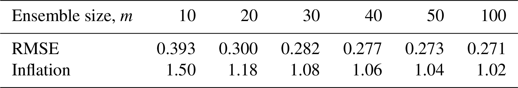
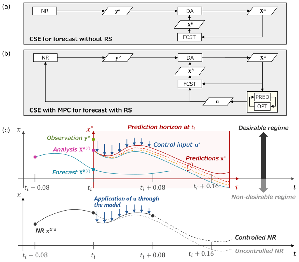
Figure 2 Flow diagram and conceptual image of the CSE with MPC. (a) Flow diagram of CSE for forecasts without a RS, which is identical to OSSE. (b) Flow diagram of the CSE with MPC for forecasts with a RS, which has additional processes for identifying and applying control inputs. (c) Conceptual image of the CSE with MPC. The upper illustration shows an image of identifying control inputs, and the lower illustration shows an application of control inputs to the NR.

3 Results and discussion

3.1 Impacts on the nature run

First, CSE is conducted with the Lorenz 63 model to verify the impacts of the MPC on the NR. The control objective is leading the system to the positive regime under the minimization of the three-variable control inputs. Here, T_p=20 steps and m=50 are selected, as discussed later in Sect. 3.2.

The NR and the L² norm of control inputs, ∥u∥, are shown in Figs. 3 and 4. The butterfly pattern appears in Fig. 3a because no control input is applied. In contrast, the NR successfully keeps the positive regime with consideration of the inequality constraint $x^{\ast }\ge \mathrm{0}$ by the MPC in Figs. 3b and 4a. This result indicates that the NR can be controlled by the short forecast (i.e., T_p=20 steps). Importantly, the value of ∥u∥ identified by the MPC is applied to the time derivative of states (i.e., $\dot{\mathit{x}})$. Therefore, the magnitude of the control inputs added to x during dt=0.01 is ∥u∥⋅dt. As demonstrated in Fig. 4b, the maximum value of the control inputs added to x during dt is approximately $\mathrm{40}\cdot \mathrm{0.01}=\mathrm{0.4}$, which is smaller than the maximum value of states.

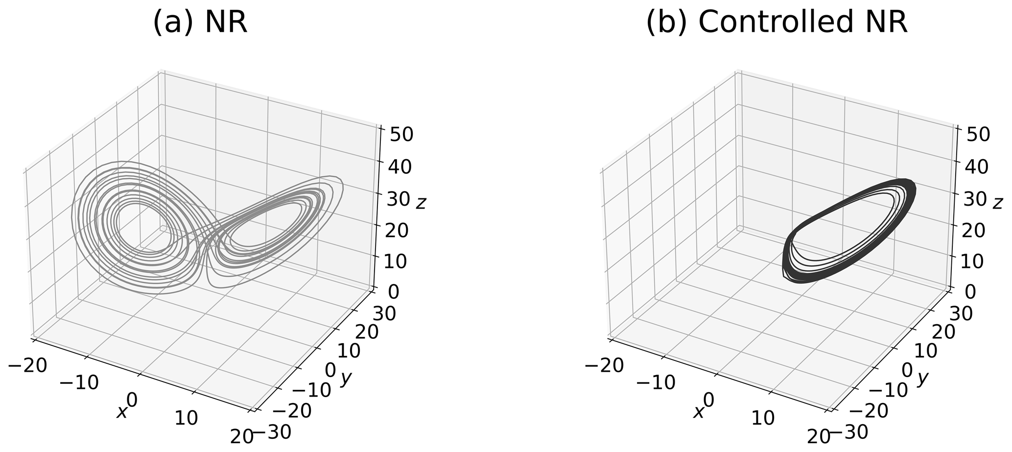
Figure 3 The NR and controlled NR of the Lorenz 63 model for 2000 steps. Each starting point is selected from the 24th step of 2 000 000-step DA cycles. Panel (a) shows the uncontrolled NR without the MPC. Panel (b) shows the controlled NR by the MPC with T_p=20 steps, T_c=8 steps, and m=50.

Figure 4 The controlled NR and the L² norm of control inputs with T_p=20 steps, T_c=8 steps, and m=50. The starting point is the 24th step of 2 000 000-step DA cycles. Panel (a) shows the time series of state x. Panel (b) shows the L² norm of control inputs, ∥u∥.

Figure 5 shows the prediction of the state and optimization of the control inputs in each horizon at an arbitrary selected step (the 232nd step of the CSE of Fig. 4). Since the forecast (dashed blue line) from the initial state shows a RS, the control is activated to solve the OCP. As demonstrated in Fig. 5a, the trajectory of the controlled prediction gradually shifts to satisfy $x^{\ast }\ge \mathrm{0}$ by iterative computations; finally, $x^{\ast }\ge \mathrm{0}$ is satisfied (solid red line). The uncontrolled NR shows a RS (dashed gray line); in contrast, the controlled NR can avoid the RS (solid black line) through the addition of control inputs (Fig. 5b, c, and d) after iterations. Note that the final prediction in the OCP and the controlled NR are not identical because the prediction in the OCP used an initial state from the member with the largest RS rather than the NR.

Figure 5 The prediction of the state and optimization of the control inputs in the horizon at an arbitrary selected step (the 232nd step of the CSE of Fig. 4). Iterative computations were performed 356 times for solving the OCP in this case. (a) The predictions, NRs, forecast, analysis, and observation in T_p. Panels (b), (c), and (d) show the control inputs $u_x^{\ast }$, $u_y^{\ast }$, and $u_z^{\ast }$ during optimization in T_c.

3.2 Sensitivity to the prediction horizon and the ensemble size

Here, we investigate the sensitivity to T_p and m for MPC performance. For that purpose, we conducted 1000 independent CSEs and summarized their SR, MTF, and MTCIs in Fig. 6. The darker color in Fig. 6 indicates better controllability. Higher values of m generally yield better results, increasing the SR and reducing MTF and MTCIs. However, improvements owing to the increased ensemble size, m, converge for m≥50 in many cases. The reasons for the improved results with larger ensemble size, m, are discussed in Sect. 3.5. In addition, the results with shorter T_p, such as T_p=10 steps, tend to be worse; the MTCIs in particular would increase because the control would be difficult by delaying the timing of control activation. On the other hand, longer T_p would not necessarily improve the results. In particular, it considerably worsens at T_p=50 steps, presumably because of discrete approximation errors involving state evolution in T_p.

It should be noted that a higher SR does not necessarily indicate lower MTF. For example, focusing on m=30, the SR of T_p=10 steps (SR=0.487) is much lower than the SR of T_p=40 steps (SR=0.921). However, the MTF of T_p=10 steps ($\mathrm{MTF}=-\mathrm{7.9}\times {\mathrm{10}}^{-\mathrm{3}})$ is lower than the MTF of T_p=40 steps ($\mathrm{MTF}=-\mathrm{2.7}\times {\mathrm{10}}^{-\mathrm{2}}$). Therefore, control would fail more frequently, but not significantly, with T_p=10 steps than with T_p=40 steps.

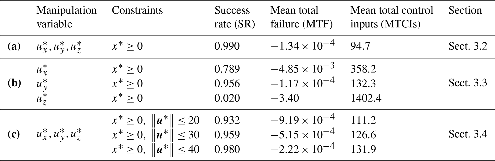
Hereafter, the experiment with T_p=20 steps and m=50 is considered to be a standard experimental setting in this study because the parameters yielded one of the best performances. The SR, MTF, and MTCIs in several experimental settings with T_p=20 steps and m=50, including the experiments discussed later (see Sect. 3.3 and 3.4), are summarized in Table 2.

Figure 6 Sensitivity to the prediction horizon, T_p, and the ensemble size, m, with three evaluation indicators: (a) success rate (SR), (b) mean total failure (MTF), and (c) mean total control inputs (MTCIs). Darker colors in (a), (b), and (c) indicate better controllability.

Table 2 Summary of the success rate (SR), mean total failure (MTF), and mean total control inputs (MTCIs) for results in each experimental setting, with T_p=20 steps and m=50 in 1000 CSEs. Row (a) shows the results of the standard MPC experiment. Row (b) shows the results of MPC experiments with only one-variable control input, and row (c) shows the results of MPC experiments with an additional constraint for the L² norm of control inputs.

3.3 MPC experiments with one-variable control input

For realistic control scenarios, it is important to consider control problems in which limited control inputs relative to model dimensions are available. Here, this section investigates the CSE with one-variable control input.

Figure 7a, b, and c show the NRs controlled only by u_x, u_y, or u_z, respectively. While the NR controlled by u_x (Fig. 7a) shows a pattern fluctuating around x=0, the NR controlled by u_y (Fig. 7b) exhibits a pattern similar to the case of three-variable control inputs (Fig. 3b). Intriguingly, the NR controlled by u_z demonstrates an unstable pattern that does not significantly deviate from x≥0. In addition, the SR, MTF, and MTCIs for the 1000 CSEs are listed in Table 2b. Compared with the case of three-variable control inputs presented in Table 2a, the case with only u_y is slightly inferior yet comparable; the controllability of the case with u_x is more difficult, and the difficulty escalates further when employing u_z. In particular, the MTCIs are larger for the case with only u_y, u_x, and u_z, in that order. Therefore, the NR controlled by u_x slightly fluctuates in the x direction, and the NR controlled by u_z significantly fluctuates in the z direction.

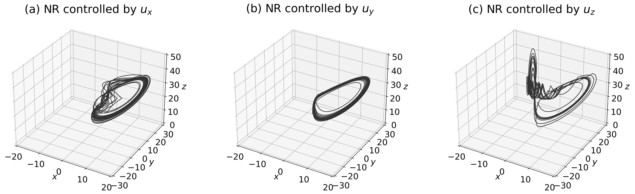
Figure 7 The NRs controlled by one-variable control input: (a) controlled by u_x, (b) controlled by u_y, and (c) controlled by u_z. Each starting point is identical to Fig. 3 (i.e., the 24th step of 2 000 000-step DA cycles).

3.4 MPC experiments constrained by magnitudes of control inputs

Here, we show that the MPC can consider constraints for control inputs in addition to the constraint for state (i.e., $x^{\ast }\ge \mathrm{0})$. Therefore, we consider MPC experiments with additional inequality constraints: the L² norm of the control inputs $∥{\mathit{u}}^{\ast }∥\le U$ $\left(U=\mathrm{20},\mathrm{30},\mathrm{40}\right)$. Namely, this section discusses MPC experiments constrained by the magnitude of control inputs. For that purpose, this study also treats $∥{\mathit{u}}^{\ast }∥\le U$ with the penalty method whose function is given by

$$\begin{array}{}\text{(32)}& P_{∥{\mathit{u}}^{\ast }∥\le U}\left(∥{\mathit{u}}^{\ast }∥\right):={\displaystyle \frac{\mathrm{1}}{\mathrm{2}}}{\left\{\max \left(∥{\mathit{u}}^{\ast }∥-U,\mathrm{0}\right)\right\}}^{\mathrm{2}}.\end{array}$$

In this study, ${\mathit{\alpha }}_{∥{\mathit{u}}^{\ast }∥\le U}={\mathrm{10}}^{\mathrm{3}}$ is selected as the penalty parameter for $∥{\mathit{u}}^{\ast }∥\le U$ from our preliminary experiments.

Figure 8 shows the NRs and the L² norm of the control inputs with additional $∥{\mathit{u}}^{\ast }∥\le U$. In all cases of U, the NRs (Fig. 8a, c, and e) indicate patterns similar to the case without $∥{\mathit{u}}^{\ast }∥\le U$ (Fig. 3b). The L² norm of the control inputs, ∥u^∗∥, satisfies the constraint for each U (Fig. 8b, d, and f), especially for a larger U. However, with a smaller U (i.e., U=20), the L² norm of control inputs occasionally exceeds the prescribed upper limit significantly. This is because the penalty method adds a penalty weighted by ${\mathit{\alpha }}_{∥{\mathit{u}}^{\ast }∥\le U}$ to the cost function and does not guarantee satisfying the constraint every time. Therefore, different results can be obtained by adjusting ${\mathit{\alpha }}_{∥{\mathit{u}}^{\ast }∥}$. For example, by increasing ${\mathit{\alpha }}_{∥{\mathit{u}}^{\ast }∥}$, $∥{\mathit{u}}^{\ast }∥\le U$ can be more strictly satisfied instead of decreasing the weight for $x^{\ast }\ge \mathrm{0}$. The SR, MTF, and MTCIs for the 1000 CSEs are presented in Table 2c. Compared with the result in the absence of $∥{\mathit{u}}^{\ast }∥\le U$ listed in Table 2a, the result with $∥{\mathit{u}}^{\ast }∥\le U$ is worse overall because the constraint imposes more difficulty on the control problem. In addition, the MTCIs decrease for a smaller U, but the SR and MTF do worsen accordingly.

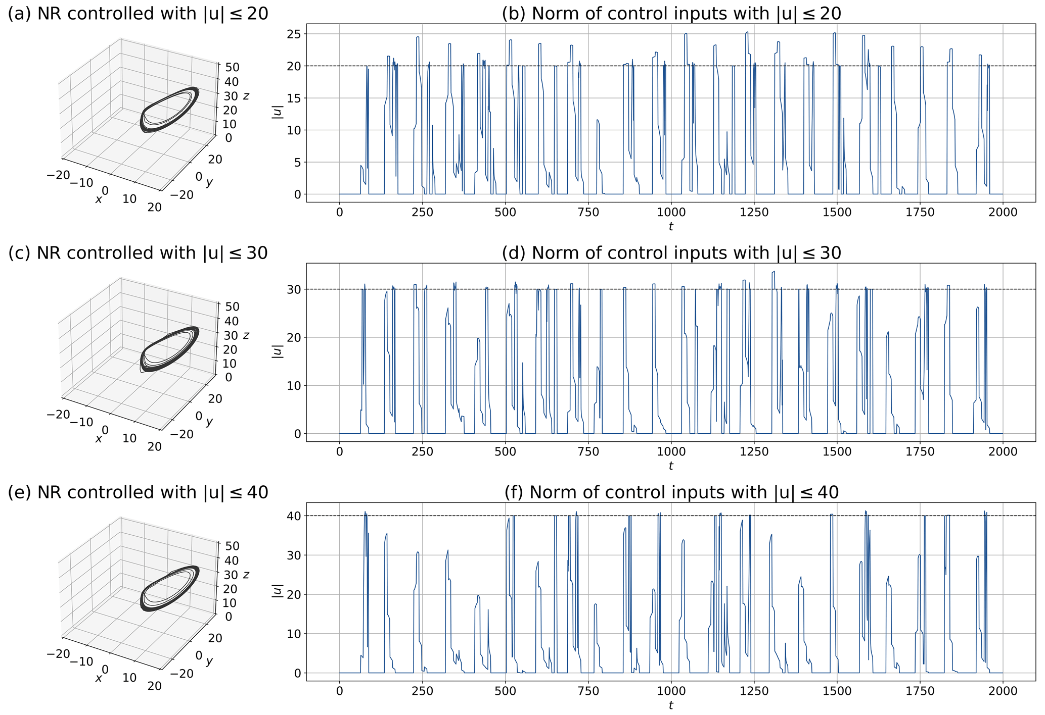
Figure 8 MPC experiments with inequality constraints for control inputs with $∥{\mathit{u}}^{\ast }∥\le U$: (a, b) U=20, (c, d) U=30, and (e, f) U=40. Panels (a), (c), and (e) show the NRs, and panels (b), (d), and (f) show the L² norm of control inputs. The dashed lines in panels (b), (d), and (f) show the prescribed upper limits of the control inputs (i.e., U=20, 30, and 40). Each starting point is identical to Fig. 3 (i.e., the 24th step of 2 000 000-step DA cycles).

3.5 Sensitivity to the initial state

For controlling NRs, it would be preferable to use the NR as the initial state for identifying control inputs. However, the state estimated by DA must be used because the true value is always unknown. Therefore, there is uncertainty in MPC-derived control inputs based on the states estimated by DA. This uncertainty may not cause serious problems for some systems without strong nonlinearity. Chaotic dynamical systems, however, require careful explorations of options for stable control because small uncertainties can cause large differences. Here, we discuss the initial state that would be valid for leading a chaotic dynamical system to a prescribed regime.

We performed 1000 independent CSEs and computed the SR, MTF, and MTCIs for five kinds of initial states: random (all mem.), mean (all mem.), random (RS mem.), mean (RS mem.), and largest (RS mem.), respectively. The (all mem.) label denotes selection among all members in the analysis ensemble, and the (RS mem.) label denotes selection among the members of the analysis ensemble showing RSs. The random label denotes a randomly sampled member, the mean label denotes the mean of the members, and the largest label denotes the member showing the largest RS. For example, mean (all mem.) indicates the mean analysis ensemble. The results are shown in Fig. 9. The experiment with the largest (RS mem.) state yielded the best results, showing the highest SR and the smallest MTF and MTCIs. Furthermore, Fig. 9 shows that it is better to use a member selected from the (RS mem.) group rather than (all mem.) as the initial state. We presume that it is safer to select a member showing a larger RS for the initial state when uncertainty exists in initial state. Therefore, the improvement with a larger ensemble size, m, in Sect. 3.2 is attributed to the fact that a larger ensemble size, m, can provide a member with a larger RS. Consequently, obtaining a member with a larger RS would be important for successfully leading chaotic dynamical systems to the prescribed regime by the MPC.

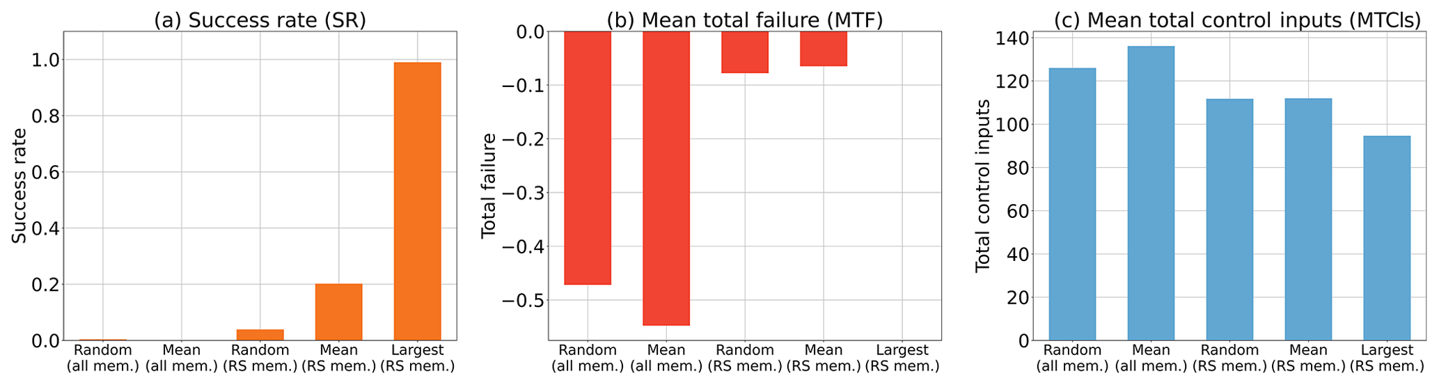
Figure 9 Sensitivity to the initial state, with T_p=20 steps and m=50. Three evaluation indicators are shown for (a) success rate (SR), (b) mean total failure (MTF), and (c) mean total control inputs (MTCIs), respectively. The (all mem.) label denotes selection from among all members in the analysis ensemble, and the (RS mem.) label denotes selection from among the members of the analysis ensemble showing RSs. The Random label denotes a randomly sampled member, the Mean label denotes the mean of the members, and the Largest label denotes the member showing the largest RS.

4 Conclusions

In this study, we propose introducing the MPC within the framework of CSE. The advantage of using the MPC is that control objectives and constraints can be explicitly considered. Therefore, we expect that this approach will be useful for realistic weather control by designing a suitable cost function and constraints.

We conducted MPC experiments with the Lorenz 63 model and successfully led the system to the positive regime. The previous CSE studies (MS22 and OTK23) required longer forecasts (about 300 steps) for successful controls with the Lorenz 63 model, whereas our approach required much shorter forecasts, such as with 20 steps. We also confirmed that controllability would be difficult with limited variables of control inputs or with additional constraints. In our discussion, we suggest that it is safer to select a member showing a larger RS for the initial state when dealing with uncertainty in initial states.

This study is an investigation of the first phase of the MPC for weather control. In the future, this approach will be investigated with more realistic NWP models. In addition, several improvements remain for the MPC to be applied to weather control. Our present approach requires many iterations to solve the OCP, and temporal forward and backward computations are required for each iteration. This means that it is computationally difficult to apply the present approach to high-dimensional NWP models as it is. Therefore, further studies are needed to explore faster approaches to solve OCPs for high-dimensional models. For this challenge, we expect the continuation/generalized minimal residual (C/GMRES) method (Ohtsuka, 2004) and quantum annealing (Inoue and Yoshida, 2020) to be fast solvers for the MPC. Furthermore, we need to consider a variety of uncertainties such as model errors and weather shifts during identifying control inputs. Therefore, uncertainty quantification is also an important research topic prior to real-world field experiments.

Finally, we emphasize caution in weather control research. The achievement of control for extreme events would be an innovative way to mitigate weather-induced disasters. However, the side effects of weather control must be carefully examined from an ethical, legal, and social issues (ELSI) perspective. In particular, we need to discuss not only the destructive side effects caused by control failures, but also the impact on biodiversity and many industries (e.g., electricity production). Our research program also addresses such social issues with legal and ethical researchers. Further ELSI research will also be conducted to satisfy responsible and innovative research for weather control studies.

Appendix A: Derivation of the necessary conditions for the optimal control input

Here, we derive the necessary conditions for optimal control inputs. For simplicity, we consider the following problem:

$$\begin{array}{}\text{(A1)}& {\displaystyle }\begin{array}{rl}\mathrm{minimize}J\left({\mathit{x}}^{\ast },{\mathit{u}}^{\ast }\right)& =\mathit{\phi }\left({\mathit{x}}^{\ast }\left(T;t\right)\right)\\ & +\underset{\mathrm{0}}{\overset{T}{\int }}L\left({\mathit{x}}^{\ast }\left(\mathit{\tau };t\right),{\mathit{u}}^{\ast }\left(\mathit{\tau };t\right)\right)\mathrm{d}\mathit{\tau },\end{array}\text{(A2)}& {\displaystyle }\mathrm{subject}\mathrm{to}\left\{\begin{array}{l}f\left({\mathit{x}}^{\ast }\left(\mathit{\tau };t\right),{\mathit{u}}^{\ast }\left(\mathit{\tau };t\right)\right)-{\dot{\mathit{x}}}^{\ast }\left(\mathit{\tau };t\right)=\mathit{0},\\ {\mathit{x}}^{\ast }\left(\mathrm{0};t\right)=\mathit{x}\left(t\right),\\ \mathit{c}\left({\mathit{x}}^{\ast }\left(\mathit{\tau };t\right),{\mathit{u}}^{\ast }\left(\mathit{\tau };t\right)\right)=\mathit{0}.\end{array}\right.\end{array}$$

A Lagrangian function is introduced to convert the constrained problem to an unconstrained problem. The Lagrangian is defined as

$$\begin{array}{}\text{(A3)}& \begin{array}{rl}\stackrel{\mathrm{̃}}{J}\left({\mathit{x}}^{\ast },{\dot{\mathit{x}}}^{\ast },{\mathit{u}}^{\ast },{\mathit{\lambda }}^{\ast },{\mathit{\rho }}^{\ast }\right)& :=J\left({\mathit{x}}^{\ast },{\mathit{u}}^{\ast }\right)\\ & +\underset{\mathrm{0}}{\overset{T}{\int }}\left\{{\left({\mathit{\lambda }}^{\ast }\right)}^T\left\{f\left({\mathit{x}}^{\ast },{\mathit{u}}^{\ast }\right)-{\dot{\mathit{x}}}^{\ast }\right\}\right.\\ & \left.+{\left({\mathit{\rho }}^{\ast }\right)}^T\mathit{c}\left({\mathit{x}}^{\ast },{\mathit{u}}^{\ast }\right)\right\}\mathrm{d}\mathit{\tau }.\end{array}\end{array}$$

In addition, a Hamiltonian is defined as follows:

$$\begin{array}{}\text{(A4)}& \begin{array}{rl}H\left({\mathit{x}}^{\ast },{\mathit{u}}^{\ast },{\mathit{\lambda }}^{\ast },{\mathit{\rho }}^{\ast }\right)& :=L\left({\mathit{x}}^{\ast },{\mathit{u}}^{\ast }\right)+{\left({\mathit{\lambda }}^{\ast }\right)}^{T}f\left({\mathit{x}}^{\ast },{\mathit{u}}^{\ast }\right)\\ & +{\left({\mathit{\rho }}^{\ast }\right)}^T\mathit{c}\left({\mathit{x}}^{\ast },{\mathit{u}}^{\ast }\right).\end{array}\end{array}$$

$\stackrel{\mathrm{̃}}{J}$ is then represented using H; it is divided into ${\dot{\mathit{x}}}^{\ast }$ terms and other terms in the integral as follows:

$$\begin{array}{}\text{(A5)}& \begin{array}{rl}\stackrel{\mathrm{̃}}{J}& \left({\mathit{x}}^{\ast },{\dot{\mathit{x}}}^{\ast },{\mathit{u}}^{\ast },{\mathit{\lambda }}^{\ast },{\mathit{\rho }}^{\ast }\right)=\mathit{\phi }\left({\mathit{x}}^{\ast }\left(T;t\right)\right)\\ & +\underset{\mathrm{0}}{\overset{T}{\int }}\left\{H\left({\mathit{x}}^{\ast },{\mathit{u}}^{\ast },{\mathit{\lambda }}^{\ast },{\mathit{\rho }}^{\ast }\right)-{\left({\mathit{\lambda }}^{\ast }\right)}^T{\dot{\mathit{x}}}^{\ast }\right\}\mathrm{d}\mathit{\tau }.\end{array}\end{array}$$

The stationary condition of $\stackrel{\mathrm{̃}}{J}$, which does not have constraints explicitly, is equal to the stationary condition of the original constrained problem. Namely, the original constrained problem was converted to an unconstrained problem. We note that this is not valid for special cases in which the linear independence constraint qualification is not satisfied. The stationary condition of $\stackrel{\mathrm{̃}}{J}$ is that its variation, $\mathit{\delta }\stackrel{\mathrm{̃}}{J}$ (i.e., infinitesimal change), is zero. After applying the Taylor expansion and disregarding higher-than-second-order terms of δx^∗ and δu^∗, $\mathit{\delta }\stackrel{\mathrm{̃}}{J}$ is given by

$$\begin{array}{}\text{(A6)}& \begin{array}{rl}\mathit{\delta }\stackrel{\mathrm{̃}}{J}& =\stackrel{\mathrm{̃}}{J}\left({\mathit{x}}^{\ast }+\mathit{\delta }{\mathit{x}}^{\ast },{\dot{\mathit{x}}}^{\ast }+\mathit{\delta }{\dot{\mathit{x}}}^{\ast },{\mathit{u}}^{\ast }+\mathit{\delta }{\mathit{u}}^{\ast },{\mathit{\lambda }}^{\ast },{\mathit{\rho }}^{\ast }\right)\\ & -\stackrel{\mathrm{̃}}{J}\left({\mathit{x}}^{\ast },{\dot{\mathit{x}}}^{\ast },{\mathit{u}}^{\ast },{\mathit{\lambda }}^{\ast },{\mathit{\rho }}^{\ast }\right)\\ & ={\left({\displaystyle \frac{\partial \mathit{\phi }\left({\mathit{x}}^{\ast }\left(T;t\right)\right)}{\partial \mathit{x}}}\right)}^T\mathit{\delta }{\mathit{x}}^{\ast }\left(T;t\right)\\ & +\underset{\mathrm{0}}{\overset{T}{\int }}\left\{{\left({\displaystyle \frac{\partial H\left({\mathit{x}}^{\ast },{\mathit{u}}^{\ast },{\mathit{\lambda }}^{\ast },{\mathit{\rho }}^{\ast }\right)}{\partial \mathit{x}}}\right)}^T\mathit{\delta }{\mathit{x}}^{\ast }\right.\\ & \left.+{\left({\displaystyle \frac{\partial H\left({\mathit{x}}^{\ast },{\mathit{u}}^{\ast },{\mathit{\lambda }}^{\ast },{\mathit{\rho }}^{\ast }\right)}{\partial \mathit{u}}}\right)}^T\mathit{\delta }{\mathit{u}}^{\ast }-{\left({\mathit{\lambda }}^{\ast }\right)}^T\mathit{\delta }{\dot{\mathit{x}}}^{\ast }\right\}\mathrm{d}\mathit{\tau }\\ & =\left\{{\left({\displaystyle \frac{\partial \mathit{\phi }\left({\mathit{x}}^{\ast }\left(T;t\right)\right)}{\partial \mathit{x}}}\right)}^T-{\left({\mathit{\lambda }}^{\ast }\left(T;t\right)\right)}^T\right\}\\ & \cdot \mathit{\delta }{\mathit{x}}^{\ast }\left(T;t\right)+{\left({\mathit{\lambda }}^{\ast }\left(\mathrm{0};t\right)\right)}^T\mathit{\delta }{\mathit{x}}^{\ast }\left(\mathrm{0};t\right)\\ & +\underset{\mathrm{0}}{\overset{T}{\int }}\left\{\left({\left({\displaystyle \frac{\partial H\left({\mathit{x}}^{\ast },{\mathit{u}}^{\ast },{\mathit{\lambda }}^{\ast },{\mathit{\rho }}^{\ast }\right)}{\partial \mathit{x}}}\right)}^T\right.\right.\\ & \left.\left.+{\left({\dot{\mathit{\lambda }}}^{\ast }\right)}^T\right)\mathit{\delta }{\mathit{x}}^{\ast }+{\left({\displaystyle \frac{\partial H\left({\mathit{x}}^{\ast },{\mathit{u}}^{\ast },{\mathit{\lambda }}^{\ast },{\mathit{\rho }}^{\ast }\right)}{\partial \mathit{u}}}\right)}^T\mathit{\delta }{\mathit{u}}^{\ast }\right\}\mathrm{d}\mathit{\tau }.\end{array}\end{array}$$

Importantly, $\mathit{\delta }{\mathit{x}}^{\ast }\left(\mathrm{0};t\right)=\mathrm{0}$ because ${\mathit{x}}^{\ast }\left(\mathrm{0};t\right)$ is fixed by x(t). In addition, δλ^∗ and δρ^∗ are disregarded because consideration of these variations only yields already obtained conditions (i.e., $f\left({\mathit{x}}^{\ast }\left(\mathit{\tau };t\right),{\mathit{u}}^{\ast }\left(\mathit{\tau };t\right)\right)-{\dot{\mathit{x}}}^{\ast }\left(\mathit{\tau };t\right)=\mathit{0}$ and $\mathit{c}\left({\mathit{x}}^{\ast }\left(\mathit{\tau };t\right),{\mathit{u}}^{\ast }\left(\mathit{\tau };t\right)\right)=\mathit{0}$). According to Eq. (A6), the condition for $\mathit{\delta }\stackrel{\mathrm{̃}}{J}$ to be zero is that the coefficients of δx^∗ and δu^∗ are zero. By summarizing the conditions from Eq. (A6), the equation of state, and the other constraints, the necessary conditions for optimal control inputs can be derived as follows:

$$\begin{array}{}\text{(A7)}& {\displaystyle }{\dot{\mathit{x}}}^{\ast }\left(\mathit{\tau };t\right)=f\left({\mathit{x}}^{\ast }\left(\mathit{\tau };t\right),{\mathit{u}}^{\ast }\left(\mathit{\tau };t\right)\right),\text{(A8)}& {\displaystyle }{\mathit{x}}^{\ast }\left(\mathrm{0};t\right)=\mathit{x}\left(t\right),\text{(A9)}& {\displaystyle }{\dot{\mathit{\lambda }}}^{\ast }\left(\mathit{\tau };t\right)=-{\displaystyle \frac{\partial H\left({\mathit{x}}^{\ast },{\mathit{u}}^{\ast },{\mathit{\lambda }}^{\ast },{\mathit{\rho }}^{\ast }\right)}{\partial \mathit{x}}},\text{(A10)}& {\displaystyle }{\mathit{\lambda }}^{\ast }\left(T;t\right)={\displaystyle \frac{\partial \mathit{\phi }\left({\mathit{x}}^{\ast }\left(T;t\right)\right)}{\partial \mathit{x}}},\text{(A11)}& {\displaystyle \frac{\partial H\left({\mathit{x}}^{\ast },{\mathit{u}}^{\ast },{\mathit{\lambda }}^{\ast },{\mathit{\rho }}^{\ast }\right)}{\partial \mathit{u}}}=\mathit{0},\text{(A12)}& {\displaystyle }\mathit{c}\left({\mathit{x}}^{\ast }\left(\mathit{\tau };t\right),{\mathit{u}}^{\ast }\left(\mathit{\tau };t\right)\right)=\mathit{0}.\end{array}$$

Appendix B: MPC experiments with starting points around the large x

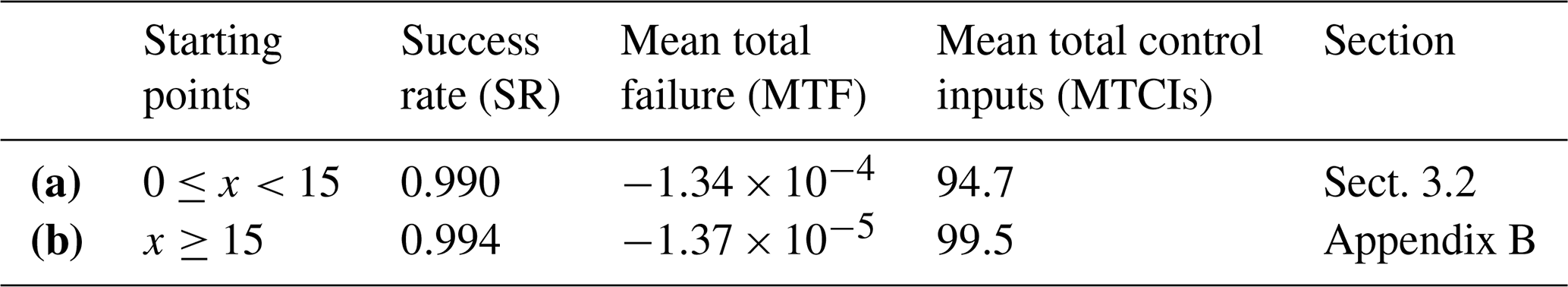
The Lorenz 63 system is known to increase the amplitude of x before RSs (e.g., Fig. 2 of MS22 and OTK23). Therefore, it is more difficult to prevent RSs for CSEs starting from a larger x. OTK23 investigated the influence of starting points in the previous CSE approach. Their result showed that the number of successes for preventing the initial RS is almost zero when the CSEs start from x≥15. Here, we investigate CSEs starting from x≥15 with our approach. The experiment setting in this appendix is the same as in Sect. 3.2, except for the starting points.

Table B1 compares the SR, MTF, and MTCIs of 1000 independent CSEs for two starting point settings (i.e., $\mathrm{0}\le x<\mathrm{15}$ and x≥15). This result shows that the controllability of the case for x≥15 (Table B1 b) is almost equivalent to the case for $\mathrm{0}\le x<\mathrm{15}$ (Table B1a). This is because the proposed method requires short forecasts with, e.g., 20 steps to lead the system to the positive regime, in contrast to the previous CSE approach (MS22 and OTK23) that requires longer forecasts with, e.g., about 300 steps. This is a promising result, showing improved controllability compared to the previous CSE approach.

Table B1 Comparison of the success rate (SR), mean total failure (MTF), and mean total control inputs (MTCIs) for two starting point settings, with T_p=20 steps and m=50 in 1000 CSEs. Row (a) shows the results of the MPC experiment whose starting points are $\mathrm{0}\le x<\mathrm{15}$. Row (b) shows the results of the MPC experiment whose starting points are x≥15.