Selecting and weighting dynamical models using data-driven approaches

In geosciences, multi-model ensembles are helpful to explore the robustness of a range of results. To obtain a synthetic and improved representation of the studied dynamic system, the models are usually weighted. The simplest method, namely the model democracy, gives equal weights to all models, while more advanced approaches base weights on agreement with available observations. Here, we focus on determining weights for various versions of an idealized model of the Atlantic Meridional Overturning Circulation. This is done by assessing their performance against synthetic observations (generated from one of the model versions) within a data assimilation framework using the ensemble Kalman filter (EnKF). In contrast to traditional data assimilation, we implement data-driven forecasts using the analog method based on catalogs of short-term trajectories. This approach allows us to efficiently emulate the model's dynamics while keeping computational costs low. For each model version, we compute a local performance metric, known as the contextual model evidence, to compare observations and model forecasts. This metric, based on the innovation likelihood, is sensitive to differences in model dynamics and considers forecast and observation uncertainties. Finally, the weights are calculated using both model performance and model co-dependency and then evaluated on averages of long-term simulations. Results show good performance in identifying numerical simulations that best replicate observed short-term variations. Additionally, it outperforms benchmark approaches such as strategies based on model democracy or climatology when reconstructing missing distributions. These findings encourage the application of the proposed methodology to more complex datasets in the future, like climate simulations.

1 Introduction

In the geosciences, several numerical models are usually available to represent the same complex system. For example, the Earth's global climate system is implemented in a range of different numerical models that are, for some, gathered within the Couple Model Intercomparison Project (CMIP; Eyring et al., 2016). Due to the different parameterizations (related to unresolved processes and numerical implementations), and given particular structural equations, a model represents an imperfect image of the studied system. In other words, each model is characterized by its own strengths and weaknesses, which impact its predictive skills. The use of the multi-model ensemble (MME) to predict a specific climate variable is then considered more informative than any individual model. Here, the models are assumed to complement each other using MME, which has the potential to improve climate system representation (Abramowitz et al., 2019).

Nevertheless the question of how to gather the information produced by the range of models remains. In this context, it is usual to follow a model democracy approach, giving equal weight to all models to enhance the representativeness. This is what is mostly done in the 6th Assessment Report (AR6) of the Intergovernmental Panel on Climate Change (IPCC, 2021). However, this strategy has been debated in the community due to the strong assumptions it implies: equal probability of all models to represent all variables in the whole phase space of the system and independence between them (e.g., Knutti, 2010; Sanderson et al., 2015; Knutti et al., 2019).

A trade-off between MME-based model democracy and selecting a single model would be to weight-average the models. The weights can be found through model performance, which consists in evaluating the consistency between model simulations and available observations. This procedure should be adapted to the specificities of model simulations being processed (Eyring et al., 2019). In particular, the models are characterized by nonlinearities which can significantly influence trajectories over short timescales. Hence, the dynamic behavior of the system needs to be properly taken into account. This can be done, for example, by assessing the models' ability to describe successive sequences of observations. In addition, the weights should account for the degree of dependency between the models, as they usually share some elements in their structure or parameterizations (Knutti et al., 2010; Abramowitz et al., 2019). Several approaches have been suggested to measure the model–observation consistency and thus obtain the individual model weights.

The first approaches are based on descriptive statistics. This is the case of “reliability ensemble averaging” (Giorgi and Mearns, 2002) and the “ClimWIP method” (Climate model Weighting by Independence and Performance; Sanderson et al., 2015 and Knutti et al., 2017). In those two methods, weights are based on the ability of model simulations to reproduce observed statistical diagnostics for one or more variables (e.g., mean, variability, or trend fields), while including a component that measures inter-model dependence. However, the score formalism does not evaluate how the models reproduce sequences of observations (which reflect model dynamics). The ClimWIP method was applied in numerous studies at global or regional spatial scales with a range of climate variables such as atmospheric temperatures or precipitations (Sanderson et al., 2015; Sanderson et al., 2017; Brunner et al., 2019, 2020; Merrifield et al., 2020), Arctic sea ice (Knutti et al., 2017), or Antarctic ozone depletion (Amos et al., 2020).

Second approaches are included in a probabilistic Bayesian framework, such as “Bayesian model averaging” (BMA; e.g., Raftery et al., 2005; Min et al., 2007; Sexton et al., 2012; Olson et al., 2016, 2019) and “kriging” methods applied at global and local scale (Ribes et al., 2021, 2022). In BMA, the distributions of model outputs are updated using available observations to obtain a posterior weighted distribution. The weights for candidate models are determined using Bayes' theorem, which combines prior beliefs (typically uniform weights) with the global likelihood of the observations estimated for each model. These weights reflect the confidence in each model considering both the data and uncertainty. However, evaluating model consistency over time is tricky because the distributions involve time-aggregated quantities for large time periods, making it less suitable for exploiting information about model dynamics.

In this study, we evaluate the performance of competing models based on their ability to reproduce short-term dynamics of the system described by observed sequences. To achieve this, a data-driven approach is adopted within a data assimilation framework (Ruiz et al., 2022). One of the main advantages is the use of already existing simulations to produce free-model probabilistic forecasts (i.e., without having to rerun the models, which greatly reduces the computational cost), while retaining the useful properties of data assimilation (Lguensat et al., 2017). The data-driven forecasts are estimated using regression based on the classic least squares but applied locally in the phase space, to capture the nonlinearities in the evolution of the system (Platzer et al., 2021). The proposed methodology is relevant for various reasons. It effectively combines the advantages of multiple weighting methods mentioned earlier. Moreover, it is integrated within a data assimilation framework, enabling a thorough consideration of the described dynamics. Also, it is written in a Bayesian framework (as BMA and kriging strategies), where data-driven forecasts are considered as Gaussian a priori information which are sequentially updated thanks to observations (which are also considered to be Gaussian). This provides accurate and reliable initialization for the next forecast. The difference between the data-driven forecasts and the observations allows for the computation of the innovation likelihood (e.g., Carrassi et al., 2017), which is used locally in time as a metric of model performance. The information of the local likelihood is then summarized following different score formalisms to yield weights. Finally, one of the scores takes into account the model dependency as in the formalism of ClimWIP (Knutti et al., 2017). The weights are tested by applying them to long-term simulations.

This study aims to develop a weighting methodology. As a first step, we use numerical simulations of an idealized chaotic deterministic model representing the centennial-to-millennial dynamic of the Atlantic Meridional Overturning Circulation (AMOC). The proposed alternative approach is compared to more classic approaches, such as model democracy, climatology, or a single best model.

The study is organized as follows. Section 2 details the methodological framework for obtaining model weights and applying them. Section 3 describes the numerical model and the data used to implement the methodology. Section 4 is devoted to the numerical results, and Sect. 5 concludes this study and presents some perspectives for future research.

2 Methodology

This section first describes the framework to measure the ability of a single dynamical model to fit a set of noisy observations. After applying it to an ensemble of competing models, the second part is devoted to the strategies for computing model weights and their application.

2.1 Evaluating the local performance of a dynamical model

Here, we evaluate the model performance based on its short-term dynamics. For this purpose, initialized model forecasts are crucial to estimate the accuracy of the dynamics with regards to observations. By synchronizing model forecasts to available observations, Bayesian data assimilation (DA) is a suitable framework for addressing this. DA, like Kalman filtering strategies, is commonly used to improve the estimation of the latent unknown state of a system by sequentially including the available observations (Carrassi et al., 2018). The associated state-space model is expressed as

$$\begin{array}{}\text{(1a)}& {\displaystyle }& {\displaystyle }{\mathit{x}}_k=\mathcal{M}\left({\mathit{x}}_{k-\mathrm{1}}\right)+{\mathit{\eta }}_k,\text{(1b)}& {\displaystyle }& {\displaystyle }{\mathit{y}}_k=\mathcal{H}\left({\mathit{x}}_k\right)+{\mathit{ϵ}}_k,\end{array}$$

where k is the time index, x_k is the true state, ℳ is the model propagator, η_k is the model error, y_k is the noisy observations, ℋ is the observational operator, and ϵ_k is the observation error. Equation (1a) represents the model relation between the true state and the previous state given an additive model error. Equation (1b) makes the relationship between the observations to the true state with an additive observational error.

In the classic Kalman filter, an assimilation cycle aims to sequentially update a Gaussian forecast distribution (generated by the model equations) with the information provided by the observations (also Gaussian), when available. The posterior analysis distribution is a more accurate and reliable estimation of the latent state by satisfying robust statistical properties (i.e., best linear unbiased estimator). Therefore, the forecast for the next time step benefits from this accurate initial condition. The ensemble Kalman filter (EnKF) is preferred when dealing with nonlinear systems (Evensen, 2003). At each time step, the two first moments of the Gaussian forecast distribution are approximated empirically using a Monte Carlo approach. To do this, N forecast members are generated from the same model equations, each one initialized from a sample of the previous analysis distribution. This is expressed as

$$\begin{array}{}\text{(2)}& {\mathit{x}}_{\left(j\right),k+\mathrm{1}}^{\mathrm{f}}=\mathcal{M}\left({\mathit{x}}_{\left(j\right),k}^{\mathrm{a}}\right)+{\mathit{\eta }}_{\left(j\right),k+\mathrm{1}},\end{array}$$

where j is the member sample index, ${\mathit{x}}_{\left(j\right),k+\mathrm{1}}^{\mathrm{f}}$ is the jth forecast member at time k+1, ${\mathit{x}}_{\left(j\right),k}^{\mathrm{a}}$ is the jth analysis member at the previous time k, and ${\mathit{\eta }}_{\left(j\right),k+\mathrm{1}}$ is the model error assumed to be Gaussian. In Eq. (2), ${\mathit{x}}_{\left(j\right),k}^{\mathrm{a}}$ is calculated as

$$\begin{array}{}\text{(3)}& {\mathit{x}}_{\left(j\right),k}^{\mathrm{a}}={\mathit{x}}_{\left(j\right),k}^{\mathrm{f}}+{\mathbf{K}}_k\left({\mathit{y}}_k-\mathcal{H}\left({\mathit{x}}_{\left(j\right),k}^{\mathrm{f}}\right)+{\mathit{ϵ}}_{\left(j\right),k}\right),\end{array}$$

where ϵ_(j),k is the observation error drawn from a random sample from the multivariate Gaussian with the 0-mean vector and an error covariance matrix R. The Kalman gain K_k in Eq. (3) is defined as

$$\begin{array}{}\text{(4)}& {\mathbf{K}}_k={\mathbf{P}}_k^{\mathrm{f}}{\mathbf{H}}^{\mathrm{T}}{\left({\mathbf{HP}}_k^{\mathrm{f}}{\mathbf{H}}^{\mathrm{T}}+\mathbf{R}\right)}^{-\mathrm{1}},\end{array}$$

where ${\mathbf{P}}_k^{\mathrm{f}}$ is the empirical covariance matrix of the forecast distribution at time k calculated using the EnKF j members, and H represents the tangent linear of the observation operator ℋ.

DA allows the model performance evaluation by measuring the consistency between the model forecasts and the available observations. Directly computed in a DA cycle, the contextual model evidence (CME) is defined as the log-likelihood of observations at a given time for a model, taking into account the forecast state as prior information (Carrassi et al., 2017). Larger CME is obtained for more consistency between the model forecast and observations. Under the Gaussian assumption included in the EnKF cycle, CME is approximated as follows:

$$\begin{array}{}\text{(5)}& \begin{array}{rl}& {\text{CME}}_k(\mathit{y};\mathcal{M})=-{\displaystyle \frac{\mathrm{1}}{\mathrm{2}}}\left({\mathit{y}}_k-\mathcal{H}\left({\stackrel{\mathrm{‾}}{\mathit{x}}}_k^{\mathrm{f}}\right)\right){\left({\mathbf{HP}}_k^{\mathrm{f}}{\mathbf{H}}^{\mathrm{T}}+\mathbf{R}\right)}^{-\mathrm{1}}\\ & {\left({\mathit{y}}_k-\mathcal{H}\left({\stackrel{\mathrm{‾}}{\mathit{x}}}_k^{\mathrm{f}}\right)\right)}^{\mathrm{T}}-{\displaystyle \frac{\mathrm{1}}{\mathrm{2}}}\ln \left(\text{det}\left({\mathbf{HP}}_k^{\mathrm{f}}{\mathbf{H}}^{\mathrm{T}}+\mathbf{R}\right)\right)\\ & -{\displaystyle \frac{r}{\mathrm{2}}}\ln \left(\mathrm{2}\mathit{\pi }\right),\end{array}\end{array}$$

where ${\stackrel{\mathrm{‾}}{\mathit{x}}}_k^{\mathrm{f}}$ is the empirical mean of the ensemble forecasts, and r is the number of available observations. At time k, CME is defined as a mean square error function between the forecast and the observation (represented by the term $\left({\mathit{y}}_k-\mathcal{H}\left({\stackrel{\mathrm{‾}}{\mathit{x}}}_k^{\mathrm{f}}\right)\right){\left({\mathit{y}}_k-\mathcal{H}\left({\stackrel{\mathrm{‾}}{\mathit{x}}}_k^{\mathrm{f}}\right)\right)}^{\mathrm{T}}$ in Eq. (5)), which is normalized by the covariance matrix accounting for both forecast and observation error (denoted as the term ${\left({\mathbf{HP}}_k^{\mathrm{f}}{\mathbf{H}}^{\mathrm{T}}+\mathbf{R}\right)}^{-\mathrm{1}}$ in Eq. (5)). It has been demonstrated that by considering both the prior and data uncertainty, CME exhibits greater effectiveness in selecting the accurate model from a pool of models compared to using the RMSE alone (Metref et al., 2019 and Ruiz et al., 2022).

In principle, DA formalism requires access to the numerical model to propagate the state of the system in order to obtain the forecasts. When performing EnKF, a large number of model forecasts are generated, representing a significant computational cost. An efficient and flexible data-driven alternative aims at combining DA with a statistical forecasting strategy based on analogs (Lorenz, 1969). In analog data assimilation (AnDA), existing long-term simulations are used instead of performing new sequential model simulations (Tandeo et al., 2015; Lguensat et al., 2017). The simulations are decomposed as a catalog of short-term trajectories (i.e., pairs of analog states and their successors) sampling the short-term model dynamics. Hence, using an appropriate distance, the analog states closest to the assimilated state are selected from the catalog. Their successors are combined using a statistical operator to obtain probabilistic forecasts. Hence, AnDA corresponds to performing a classic DA process but replacing the model propagator by its analog-based approximation in Eq. (1a). This reads

$$\begin{array}{}\text{(6)}& {\displaystyle }{\displaystyle }{\mathit{x}}_k=\widehat{\mathcal{M}}\left({\mathit{x}}_{k-\mathrm{1}}\right)+{\mathit{\eta }}_k,\end{array}$$

where $\widehat{\mathcal{M}}$ refers to the analog-based forecasting propagator.

In practice, it consists in fitting a local linear regression (Cleveland and Devlin, 1988) relating the selected analogs to their successors, which has proven to be robust (Zhen et al., 2020; Platzer et al., 2021). The regression is able to learn the local-time dynamic of the model including nonlinearities since the linear adjustment is applied locally in the phase space. By projecting the current state with the regression, statistical approximated forecasts are obtained. The forecast takes into account the regression uncertainty (assumed Gaussian) which is a robust estimate of the model error. When the catalog is large enough (to approximately cover the full dimension of the phase space), it has been shown that AnDA performs as well as DA (Lguensat et al., 2017). Ruiz et al. (2022) have recently shown, using different idealized dynamical models, that CME can be robustly estimated using AnDA. The combination of AnDA with CME is the basis of the current study.

2.2 Strategies for model weighting average

The methodology described above is applied to an ensemble of L models in order to individually measure their forecast skills given a set of observations. For each model, CME time series are obtained and used to derive individual weights. The weights are then applied to provide a model average that is representative of the observations.

2.2.1 Calculating CME-based weights

The CME time series can be processed in various ways to obtain a single scalar (i.e., the score) used to derive the model weight. In this study, three CME scores are defined, together with three benchmark scores (not using CME). Hence, we define $w_{\text{score type}}^{\left(i\right)}$ as the score assigned to model ℳ⁽ⁱ⁾. For simplicity, the scores are here described prior to their normalization, which leads to the model weights.

• a.

  The model democracy (Knutti, 2010) gives the same weight to all models, regardless of model performance. It reads

  $$\begin{array}{}\text{(7a)}& w_{\text{democracy}}^{\left(i\right)}=\mathrm{1}.\end{array}$$
• b.

  The climatological score is based on the comparison of model and observation distributions. Here, there is no assimilation process, which means that this score does not evaluate the local dynamics. It measures the minimum cumulative value of the two histograms, highlighting the common area between both distributions. A score close to 0 denotes a model that poorly simulates the observed distribution, while a score of 1 is obtained by a model with a perfect climatological distribution (Perkins et al., 2007). It reads

  $$\begin{array}{}\text{(7b)}& w_{\text{climato}}^{\left(i\right)}=\sum _{j=\mathrm{1}}^n\text{minimum}\left(Y\right(j),M^{\left(i\right)}(j\left)\right),\end{array}$$

  where Y and M⁽ⁱ⁾ are the normalized histograms (such that their respective sum equals 1) of the observations and the model simulations, respectively, j is the index of histogram equal-width bins, and n is their total number. Note that in the current study, single-variable observations are used, but the score could be adapted using multivariate distributions.

• c.

  The single best model score assigns 1 to the model showing the best climatological score and 0 to the others. Opposite to the democracy score, it only takes into account the best-performing model over the whole set of observations (Tebaldi and Knutti, 2007). It reads

  $$\begin{array}{}\text{(7c)}& w_{\text{single}}^{\left(i\right)}=\left\{\begin{array}{ll}\mathrm{1},& \text{if}{w}_{\text{climato}}^{\left(i\right)}>w_{\text{climato}}^{\left(j\right)}\forall i\ne j;\\ \mathrm{0},& \text{otherwise}.\end{array}\right.\end{array}$$
• d.

  The CME-ClimWIP score is based on the ClimWIP approach (Knutti et al., 2017). Our adaptation reads

  $$\begin{array}{}\text{(7d)}& w_{\text{CME-ClimWIP}}^{\left(i\right)}={\displaystyle \frac{e^{\frac{D_i}{{\mathit{\sigma }}_{\mathrm{D}}}}}{\mathrm{1}+{\sum }_{j\ne i}^L{e}^{\frac{S_{ij}}{{\mathit{\sigma }}_{\mathrm{S}}}}}},\end{array}$$

  where D_i measures the intra-model performance with its associated shape parameter σ_D and S_ij measures the inter-model dependency with its associated shape parameter σ_S. D_i and S_ij are usually expressed with Euclidian distance (Knutti et al., 2017). Here, we evaluate D_i such that $D_i={\sum }_{k=\mathrm{0}}^K{\text{CME}}_k(\mathit{y};{\mathcal{M}}^{\left(i\right)})$, where K is the number of time steps, and S_ij is the sum of the defined inter-model such that $S_{ij}={\sum }_{k=\mathrm{0}}^K{\text{CME}}_k({\mathcal{M}}^{\left(i\right)};{\mathcal{M}}^{\left(j\right)}{)}_{j\ne i}$. The CME-ClimWIP score is higher if model forecasts match observations and if they are sufficiently different from other-model forecasts. The two parts of Eq. (7d) are balanced thanks to the use of the parameters σ_D and σ_S. When they are appropriately set within the score, a few top-performing models are selected. Notably, higher values for these parameters bring the score closer to the model democracy, while when σ_D=1 and ${\mathit{\sigma }}_{\mathrm{S}}\to +\mathrm{\infty }$ the BMA expression is retrieved. In particular, the numerator in Eq. (7d) corresponds to a formulation of model evidence typically calculated for model selection problems (see Appendix A for more details on this specific point). Classic ClimWIP and BMA approaches are special cases of the CME-ClimWIP score which are discussed in Sect. 4.2.3. Note that σ_D and σ_S are determined according to the specific experiment model tests following Knutti et al. (2017) and Lorenz et al. (2018).

• e.

  The CME best punctual model score exploits the local-time performance provided by CME. It assigns a local value of 1 to the best model at time k and 0 to the other models. The score reads

  $$\begin{array}{}\text{(7e)}& w_{\text{punctual}}^{\left(i\right)}={\displaystyle \frac{\mathrm{1}}{K}}\sum _{k=\mathrm{0}}^K{{\text{𝟙}}_{\mathit{\left\{}{\text{CME}}_k\right(\mathit{y};{\mathcal{M}}^{\left(i\right)})>{\text{CME}}_k(\mathit{y};{\mathcal{M}}^{\left(j\right)}\left)\mathit{\right\}}}}_{i\ne j},\end{array}$$

  where 𝟙 is the indicator function assigning 1 when the condition $\mathit{\left\{}{\text{CME}}_k\right(\mathit{y};{\mathcal{M}}^{\left(i\right)})>{\text{CME}}_k(\mathit{y};{\mathcal{M}}^{\left(j\right)}){\mathit{\}}}_{i\ne j}$ is satisfied and 0 otherwise. This score captures the good performance of model in specific regions of the phase space, despite not necessary being optimal in other regions. For example, extreme values are often only well captured by a few specific models. By retaining the information from only one model at each time k, the score bypasses the need to identify temporal inter-model similarities.

• f.

  The CME best persistent model score $w_{\text{persistent}}^{\left(i\right)}$ is derived from the previous score by overweighting models that are the best on several consecutive states. The score is linearly proportional to the cumulative number of consecutive time steps where the model is the best (expression not shown here). This score emphasizes consistently good local dynamics.

2.2.2 Assessing the performance of weighting-averages

Here, the methodology for one experiment consists in two successive stages (Fig. 1). The first step corresponds to a training stage where AnDA is applied to obtain the CME time series associated with each candidate model (left panel of Fig. 1). From them, CME-based scores are calculated following the expressions defined in Sect. 2.2.1 as well as the three benchmark scores (bottom center panel of Fig. 1). The second step is a testing stage consisting in applying the six weighting approaches on new individual model simulations and comparing their effectiveness to suitably reconstruct the true one (right panel of Fig. 1). Considering probability density functions (PDFs) of model simulations, the reconstructed PDF related to a score is calculated as follows:

$$\begin{array}{}\text{(8)}& p\left(\stackrel{\mathrm{̃}}{\mathit{\omega }}\right|{\mathcal{M}}^{\left(\mathrm{0}\right)},\mathrm{\dots },{\mathcal{M}}^{\left(L\right)},y)={\sum }_{i=\mathrm{0}}^{L}p(\stackrel{\mathrm{̃}}{\mathit{\omega }}\left|{\mathcal{M}}^{\left(i\right)}\right)\cdot w_{\text{score}}^{\left(i\right)},\end{array}$$

where $p\left(\stackrel{\mathrm{̃}}{\mathit{\omega }}\right|{\mathcal{M}}^{\left(\mathrm{0}\right)},\mathrm{\dots },{\mathcal{M}}^{\left(L\right)},y)$ denotes the reconstructed PDF of the normalized AMOC (denoted as $\stackrel{\mathrm{̃}}{\mathit{\omega }}$); $p\left(\stackrel{\mathrm{̃}}{\mathit{\omega }}\right|{\mathcal{M}}^{\left(i\right)})$ represents the individual PDF associated with model i; and $w_{\text{score}}^{\left(i\right)}$ is the weight of model i for a given score, depending on y the set of observations. To evaluate the skill of the reconstructed PDF, its overlap (in terms of %) with the PDF of the truth is calculated (following a similar formalism to that of the climatological score $w_{\text{climato}}^{\left(i\right)}$; Eq. (7b)). The resulting reconstruction score performance for the six approaches can then be compared.

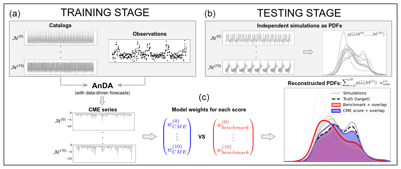
Figure 1 Schematic of the two-stage methodology for one experiment using 11 models. (a) Training stage performing AnDA with the 11 catalogs and a single set of observations leading to CME computation. (c) Model weights calculated for two illustrative scores, one based on CME and another based on a benchmark method (blue and red, respectively). (b) Individual PDFs of new model simulations (grey) are weighted following Eq. (8) to obtain a reconstructed PDF associated with both competing scores (blue and red). The quality of both reconstructions is assessed by measuring the overlap (blue and red shadings) with the true PDF (dashed black line) which allows for comparison of the performance of the two scores. Here, the CME score shows a higher overlap with the true distribution, highlighting a better reconstruction compared to the benchmark score.

3 Experimental setup

3.1 Idealized AMOC model

The study is based on an idealized autonomous low-order deterministic model of the AMOC able of reproducing its millennial variability within a chaotic dynamics (Sévellec and Fedorov, 2014, 2015). The model is derived from the long history of salinity loop-models (originally proposed by Welander, 1957, 1965, 1967; Howard, 1971; Malkus, 1972). Its formalism with three equations (Dewar and Huang, 1995, 1996; Huang and Dewar, 1996) reads

$$\begin{array}{}\text{(9a)}& {\displaystyle \frac{\text{d}\mathit{\omega }}{\text{d}t}}& {\displaystyle }=-\mathit{\lambda }\mathit{\omega }-\mathit{ϵ}\mathit{\beta }{S}_{\mathrm{NS}},\text{(9b)}& {\displaystyle \frac{\text{d}{S}_{\mathrm{BT}}}{\text{d}t}}& {\displaystyle }=\left({\mathrm{\Omega }}_{\mathrm{0}}+\mathit{\omega }\right)S_{\mathrm{NS}}-K{S}_{\mathrm{BT}}+{\displaystyle \frac{F_{\mathrm{0}}{S}_{\mathrm{0}}}{h}},\text{(9c)}& {\displaystyle \frac{\text{d}{S}_{\mathrm{NS}}}{\text{d}t}}& {\displaystyle }=-\left({\mathrm{\Omega }}_{\mathrm{0}}+\mathit{\omega }\right)S_{\mathrm{NS}}-K{S}_{\mathrm{NS}},\end{array}$$

where t is the time; ω is the variable component of the overturning circulation strength; S_BT and S_NS are the bottom-top salinity gradients and the north–south salinity gradients, respectively; Ω₀ is the steady part of the overturning circulation strength, which acknowledges the impact of constant temperature and surface winds; ϵ is the buoyancy torque; λ is a linear friction; β is the haline contraction coefficient; K is a linear damping; and $F_{\mathrm{0}}{S}_{\mathrm{0}}/h$ is the surface salt flux (where F₀ is the freshwater flux intensity; S₀ is a reference salinity; and h is the loop thickness, i.e., the depth of the level of no motion).

Equation (9a) describes the momentum balance. Here, the rate of change of the ocean overturning strength is driven by the meridional salinity gradients accounting for the buoyancy torque and a linear friction. Equations (9b) and (9c) describe the evolution of the salinity gradients driven by advection, a linear damping representative of diffusion, and the surface salt flux.

Numerical integrations are done using a fourth-order Runge–Kutta method with a time step of 1 year. All reference parameters are set following Sévellec and Fedorov (2014) (which we refer interested reader to). Their values are h=1000 m, ${\mathrm{\Omega }}_{\mathrm{0}}=-\mathrm{2.5}\times {\mathrm{10}}^{-\mathrm{2}}$ yr⁻¹, F₀=1 m yr⁻¹, S₀=35 psu, $\mathit{\lambda }={\mathrm{10}}^{-\mathrm{2}}$ yr⁻¹, ϵ=0.35 yr⁻², $K={\mathrm{10}}^{-\mathrm{4}}$ yr⁻¹, and $\mathit{\beta }=\mathrm{7}\times {\mathrm{10}}^{-\mathrm{4}}$ psu⁻¹.

3.2 Ensemble of AMOC model versions

Various versions of the AMOC model are obtained by perturbing some parameters in the equations (Ω₀, K, and $\frac{\mathit{\lambda }}{\mathit{ϵ}}$), while others remain fixed. All possible combinations between the reference values of the parameters, doubled, and halved lead to 27 distinct parameterizations. A total of 11 are selected by ignoring the versions describing singular dynamics (e.g., with strong instabilities, constant over time, or presenting periodic behavior). Thus, for the same equations, the 11 sets of parameters induce their own dynamics. These dynamics show similarities and differences that can be visualized by the computation of the trajectories in the phase space (Fig. 2).

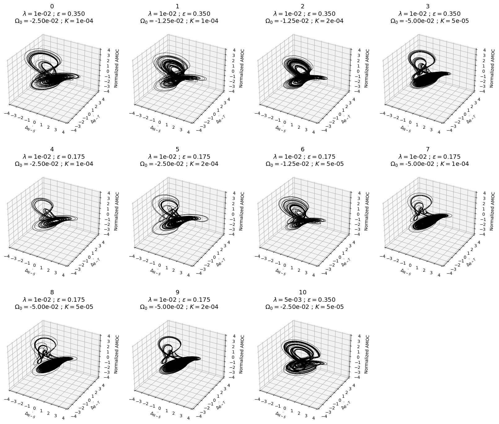
Figure 2 Chaotic trajectories in the phase space of the 11 perturbed versions of the three-variable (normalized here) AMOC model (Sévellec and Fedorov, 2014). The values of the perturbed parameters (λ, ϵ, Ω₀, and K) used to generate the 11 model versions are indicated in the title of each panel. The attractor labeled 0 (top left) corresponds to the model with the reference set of parameters.

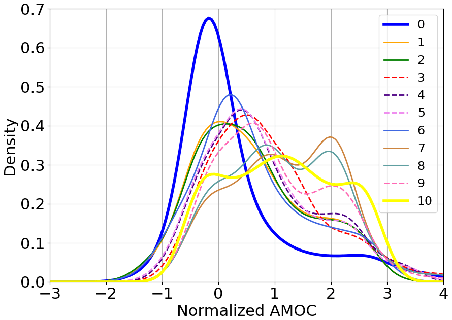
3.3 Synthetic data

A model-as-truth experiment framework is set up (e.g., Herger et al., 2018), in which one model is used to generate noisy pseudo-observations. Here, only ω is observed and will be used as the variable of interest. To efficiently select the analogs, the three variables are normalized (here rescaled). In particular, the normalized values of the original variable ω are associated with the new variable called “normalized AMOC” (Fig. 3). In all the experiments, the covariance of the observations for the normalized AMOC is fixed to R=0.5I₃. The AnDA framework is applied over a period of K=8000 years with an assimilation step of 20 years, thus resulting in 400 assimilation cycles. The choice of the assimilation step allows the forecasts to be sufficiently differentiated, so that the competing models can be distinguished locally over time when using CME (sensitivity experiments not shown). The methodology has been tested with different catalog sizes. A catalog size of 400 000 years ensures robust data-driven forecasts estimates in all the experiments. For each of the 200 EnKF members of an AnDA cycle, forecast distributions are estimated using a fixed number of 10 000 analogs. These ensure the stability of the forward propagator algorithm across all 11 experiments, particularly in areas less frequently visited. These areas are often associated with extreme values, making it more challenging to track suitable analogs (Lguensat et al., 2017).

Figure 3 Distributions of normalized AMOC for the 11 model versions.

4 Experimental results

The different methods are evaluated using two protocols. In the first one, we consider a “perfect experiment”, where the model used to generate the pseudo-observations is also included in the catalog. In the second one, the model is excluded from the catalog, and we talk about an “imperfect experiment”. For both perfect and imperfect cases, we first describe an illustrative experiment when model 8 is used as pseudo-observations and then summarized the results for each model alternately used to generate the pseudo-observations following a leave-one-out experiment design.

4.1 Perfect model experiment

The goal of the perfect model approach is to measure the ability of the three CME-based scores to retrieve the correct model (by giving it a predominant weight) from a pool of catalogs, including the true one. The skills of these scores are then compared with the skills of the three benchmarks. In all the perfect model experiments of this study, the CME-ClimWIP score is computed using the optimal values of σ_D=0.3 and σ_S=0.4, which maximize the overall overlap scores in all the experiments combined (following Knutti et al., 2017 and Lorenz et al., 2018).

4.1.1 Experiment with model 8

AnDA is performed on the 11 models with the same pseudo-observations from model 8, and CME is computed for each assimilation cycle. The resulting CME series for each individual model varies significantly over time and differs locally from model to model (Fig. 4). CME of models 0, 1, 2, 6, and 10 is more than 75 % lower than −1 (Fig. 5), showing their inefficiency to replicate model 8 system dynamics. The CME distributions of models 3, 7, and 9 show a narrower distribution, with 75 % values greater than −1. This means they are both accurate and reliable. As expected, the model with the highest and more consistent CME is model 8. This demonstrates the ability of CME to retrieve the correct model from a range of models.

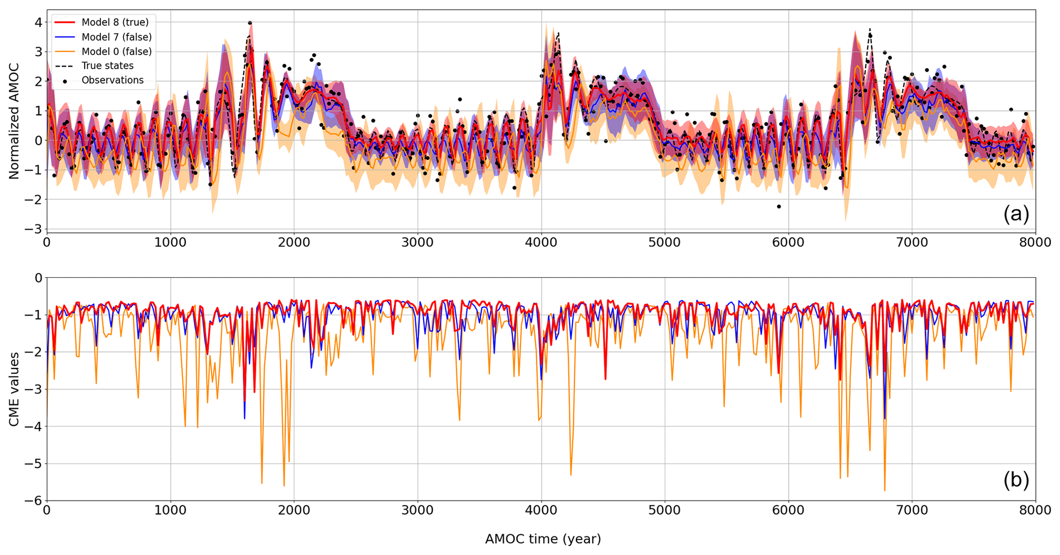
Figure 4 AnDA results on 400 cycles using model 8 to generate the pseudo-observations: examples of three assimilated models among the 11. (a) Time series of normalized AMOC with forecasts mean states and 90 % prediction interval (in shades). The red series denotes the true model (i.e., model 8), and the orange and blue ones refer to models 0 and 7, respectively. The black dots represent the noisy observations generated from the true states denoted by the dashed black line. (b) Associated CME time series for each model. Values of CME close to zero indicate better forecast distribution.

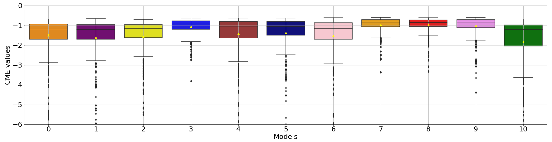
Figure 5 CME distributions from AnDA results using model 8 to generate the pseudo-observations. CME distributions are on the y axis and model number (from index 0 to 10) on the x axis. The boxes span the 25th, median, and 75th percentiles of the distributions, while the whiskers show the minimum and maximum values (excluding the outliers denoted with the black diamonds). The mean is indicated with the small yellow triangle.

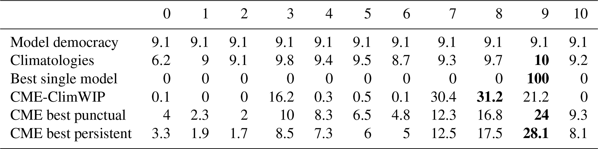
The climatology-based score produces almost uniform weights close to model democracy (Table 1). Indeed, the model climatological distributions are very comparable. This impacts the reliability of selecting a single model following the best model score. Beyond that, the observation error leads the climatology-based score to misidentify model 9 instead of model 8. The CME-ClimWIP score assigns its highest weight to the correct model, model 8, while giving significant weights to models 7 and 9. Regarding the two other CME-based scores, although the weight associated with model 8 is high, these scores give the highest weight to model 9. We conclude that the time selection characteristics of them make both scores more sensitive to observation errors.

Table 1 Perfect model results for model 8 as the pseudo-observation. For each score (in row): weights (in %) associated with the 11 models. The sum of the weights per row is 100. Values in bold highlight the model with the highest weight for each score.

4.1.2 Overall 11 experiments

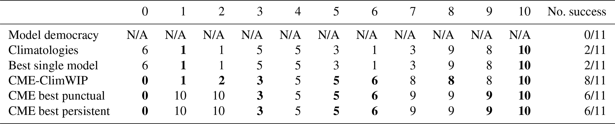
By varying the model used to generate the pseudo-observations in the 11 AnDA experiments, we can robustly assess the ability of the six scores to efficiently retrieve the correct model (Table 2). As emphasized in the specific experiment for model 8, the scores based on climatology do not allow for a clear discrimination between models. Hence the climatological and the best single model only retrieved the correct model twice over the 11 experiments (i.e., experiments with models 1 and 10). The CME-based scores perform better, attributing their highest weight to the correct model eight times for CME-ClimWIP and six times for both CME best punctual and CME best persistent. As for the model 8 experiment, in most of the unsuccessful experiments of the three CME scores, the correct model still has a weight close to the weight of the selected one (not shown here). These results emphasize that identifying the correct model is more effective using local dynamics (thanks to DA framework) rather than climatological statistics.

Table 2 Summarized perfect model results of the leave-one-out model-as-truth experiments. For each column representing an experiment (i.e., the model index used to generate pseudo-observations), the index of the model with the highest weight is specified for each score in the row. The indices in bold show when the true model is recovered. The last column summarizes how frequently the correct model is identified among the candidate models across the 11 experiments for the five scores. Note that “N/A” is indicated for model democracy since the score prevents differentiation between models.

4.2 Imperfect model experiment

The imperfect model approach aims to reconstruct the statistical properties of the distribution of a missing model using distinct models. In all the imperfect experiments of this study, the CME-ClimWIP score is computed using the optimal values of σ_D=0.5 and σ_S=0.7 which maximize the overlap scores in all the experiments combined (following Knutti et al., 2017 and Lorenz et al., 2018).

4.2.1 Experiment with model 8

The model democracy approach yields the worst reconstruction (Fig. 6, left panel), stressing that, in this case, the observation information should be included in the weight calculation. The climatology-based score slightly improves the reconstruction provided by the model democracy (+0.8 % compared to model democracy). By selecting model 9, the best single-model score improve the reconstruction of the true model 8 distribution by 6 % compared to the model democracy. The reconstructed distributions associated with the three strategies (i.e., model democracy, climatology, best single model) are all positively skewed, underestimating the true normalized AMOC (Fig. 6, left panel). The three CME-based scores outperform the three benchmark ones, with greater overlaps of their reconstruction with the truth. In particular, they all reconstruct better statistics for high positive values of normalized AMOC. For CME-ClimWIP, three models contribute the most to the reconstruction of the true missing model: model 3 by 18.1 %, model 7 by 49.1 %, and model 9 by 31.7 %. To a lesser extent, the same three models are also selected for the best punctual and best persistent scores but still leave a greater contribution from the other seven models. This suggests that the information provided by these seven models is negligible, as the two last CME strategies have lower overlapping scores than the one obtained using CME-ClimWIP.

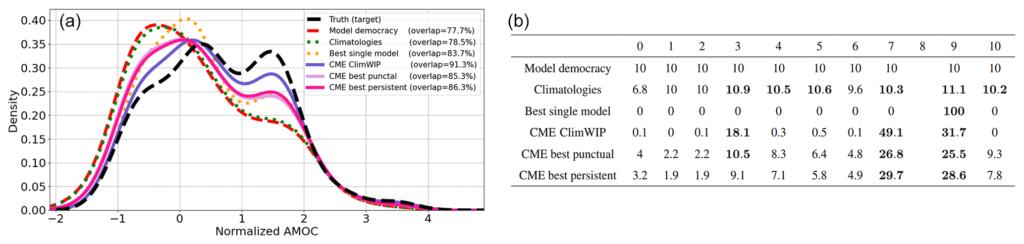
Figure 6 Imperfect model results of the model 8 experiment (by excluding it). (a) Reconstructed distribution of normalized circulation strength for the six scores with different colors. They are compared with the true distribution, shown by the dashed black lines. The overlap score (in %) for each score is expressed in the legend in brackets. (b) Table of model weights (in %) for each score (the sum of the weights per row is 100). Values in bold highlight the weights greater than the model democracy weight (> 10 %) which correspond to the models contributing the most to the distribution reconstruction.

4.2.2 Overall 11 experiments

When the 11 models are reconstructed independently in the imperfect framework, the three CME-based scores produce better reconstructions on average than the democracy and climatologies scores (Fig. 7). Similar to the specific model 8 reconstruction, the climatology comparison score does not provide meaningful distinctions between the models. This results in high variations in the reconstruction score when using the best single model across all experiments, further highlighting its unreliability. For instance, while the score effectively captures most of the distribution when reconstructing models 1 and 2 (due to their highly similar dynamics), for other experiments, it yields lower reconstruction performance. These results highlight the ability of using local-dynamics over climatology statistics for accurately differentiating between models for our reconstruction problem.

The reconstruction performances in the 11 experiments show that CME-ClimWIP greatly outperforms the model democracy for 7 of 11 model reconstructions. As for model 8 reconstruction, CME-ClimWIP gives higher weights to a small subset of models, making it well suited to reconstructing distributions that share similarities with some others in the ensemble.

On the other hand, CME-ClimWIP is close but less useful than democracy (and climatologies) for reconstructing models 3, 5, 9, and 10. Here, despite the six scores having lost performance, uniform weights are appropriate for good reconstruction. A typical example of such case is the reconstruction of model 10 whose distribution is quite symmetric, whereas all the other models have asymmetric distribution. For model 3, 5, 9, and 10 experiments, CME best punctual and persistent give better results than CME-ClimWIP. It is worth noting that these two scores also have greater reliability across all 11 experiments than CME-ClimWIP, since their reconstruction performance remains consistently superior to the model democracy score, with minimal variation between all the experiments.

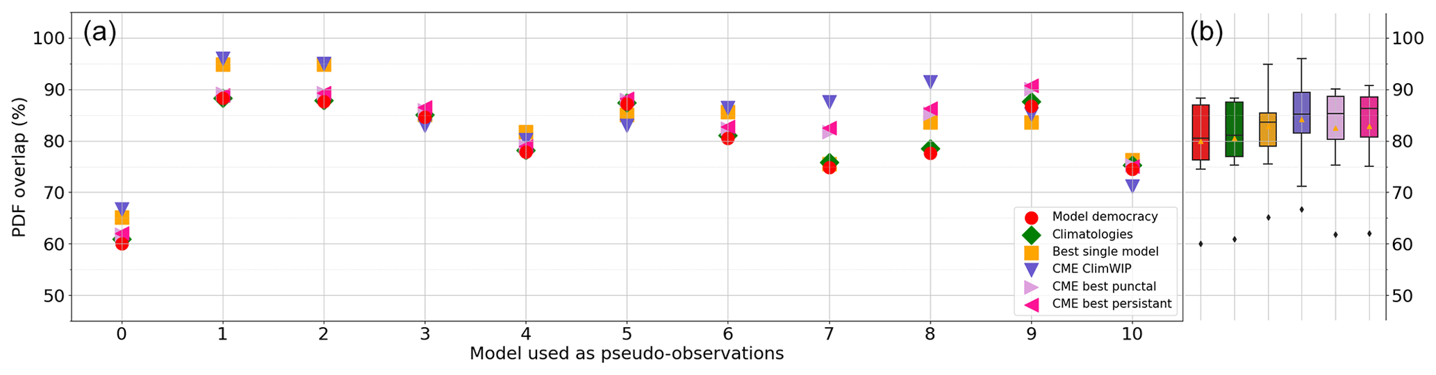
Figure 7 Imperfect model results (i.e., excluding the true model) of the leave-one-out model-as-truth experiments. (a) The model index used as pseudo-observations is on the x axis, whereas the overlap scores (in %) between the reconstructed PDF and the true PDF are read on the y axis. Each colored marker corresponds to a score strategy as denoted in the legend. (b) For each score, box plots spanning (keeping the same color code) the 25th, median, and 75th percentiles of the distributions of overlap scores for all the model-as-truth experiments combined. The whiskers show the minimum and maximum values excluding the outliers denoted with the black diamonds. Small yellow triangles indicate the means.

4.2.3 Comparing CME-ClimWIP reconstruction performance to alternative literature scores

As expressed in Eq. (7d), the CME-ClimWIP score is composed of the performance and dependence of the models, both expressed using the CME. CME at time k depends on the innovation (i.e., the difference between ${\stackrel{\mathrm{‾}}{\mathit{x}}}_k^{\mathrm{f}}$ and y_k) and the covariance error matrices ${\mathbf{P}}_k^{\mathrm{f}}$ and R. The degree of contribution of the performance and independence is controlled by two tuned shape parameters: σ_D and σ_S. Hence, to assess the importance of each component in the reconstruction performance, various versions of the CME-ClimWIP score are tested, by taking into account the influence of each component or not (Table 3). Note here that two alternative versions represent weighting strategies of the literature mentioned in the Introduction. Hence, BMA formalism (with model evidence estimated using successive CME) and the ClimWIP approach (not considering the covariance error matrix) are presented (refer to rows 5 and 6, respectively, in Table 3).

Table 3 Sensitivity of the reconstruction performance (based on overlap of the reconstruction distribution with the truth) to various alternative/simplified versions of the ClimWIP score (first column) in the imperfect model approach. The second column shows the overlap associated with the model 8 experiment. The third column shows the results of all leave-one-out experiments combined.

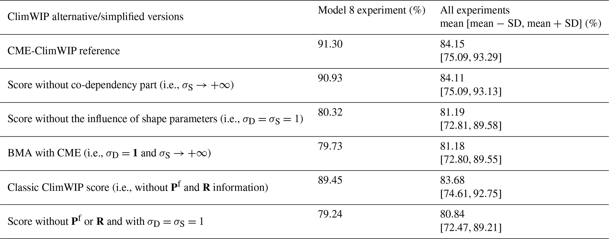
The degree of dependence between models does not contribute significantly to the reconstruction performance (Table 3). Since the 11 model versions are based on the same set of equations and the three variables are normalized, the model-model redundancy is significant. This implies that the inter-model dependency (i.e., the denominator in Eq. (7d)), is too similar across the models to contribute notably to differentiate them. The shape parameter (σ_D) has the main impact on the CME-ClimWIP by driving the score performance. The reconstruction performance of the CME-ClimWIP version without tuning the shape parameters is more than 10 % lower than the reference performance. The same conclusion can be done concerning the BMA approach. The ClimWIP score computed without information from P^f and R has lower performance than the reference, confirming the usefulness of CME (including the covariances in its formulation) over a metric only based on Euclidian distance. Finally, when both covariances and shape parameters are excluded from the score, the performance lost is even more important.

5 Conclusion and perspectives

This study aims at developing a data-driven methodology for weighting models, only based on their ability to represent the dynamics of observations. For this purpose, a set of dynamical models is compared to noisy observations, where model equations are replaced by available simulations. The method combines a machine learning approach (i.e., an analog forecasting method) to estimate the model forecasts in a cost-effective manner (i.e., without the need to re-run the model) and a sequential data assimilation algorithm (i.e., the ensemble Kalman filter). The time-varying performance of the models with respect to observations is evaluated using the contextual model evidence (also known as innovation likelihood), which benefits from DA properties.

To test this methodology, an ensemble of 11 models is obtained by perturbing parameters of an idealized chaotic model of the AMOC. For each model version, the equations are only used to generate large simulations of its three variables. Each version alternately plays the role of truth (i.e., leave-one-out experiments) used to construct pseudo-observations of the AMOC component. In the 11 experiments, model weights are extracted from the CME series using different strategies. They take into account the performance of the models with respect to pseudo-observations and the degree of similarity with other models. The method is then assessed by applying the weights to the distributions of long-term model simulations. In this way, we test the extent to which the short-term dynamics of individual models can provide relevant information for reconstructing the statistics of a targeted distribution. Reconstruction performance is measured by the percentage of overlap between the reconstructed and the true distributions. The reconstruction performance associated with the three CME-based scores is compared to three benchmark approaches that do not include DA framework (i.e., model democracy, climatological distributions comparison, and best single model).

The results of the perfect model approach highlight a better performance of CME-based scores in recovering the correct model, compared to benchmarks, suggesting the importance of using DA. The results of the benchmark strategies generally suffer from a lack of discrimination between models to correctly identify the right one. In the context of the imperfect model approach, the scores based on CME are able to reconstruct the targeted distribution more suitably than the benchmarks using the same partial noisy observations. This emphasizes the valuable information contained within the short-term dynamics, rather than the general information provided by climatological statistics, enabling efficient differentiation between models. The results underline that CME-based scores can be seen as a compromise between the “democracy score” and the so-called “dictatorial score” which selects only a single model. Within the CME-based score, the CME-ClimWIP score is relatively closer to “dictatorship”. It is suitable for reconstructing distributions sharing similarities with few models in the ensemble and when democracy is not appropriate. On the other hand, the CME best punctual and CME persistent scores are closer to “democracy”. By exploiting temporal performance, their weights are more adaptive, which is advantageous for outperforming the already successful democracy in any experiment (when CME-ClimWIP does not succeed).

An inherent assumption of our study is the Gaussianity of the EnKF forecast distributions. Testing its validity through a Jarque–Bera test (Jarque and Bera, 1980), we find that it is valid for up to 50.5 % of the 400 total forecasts for model 0 and pseudo-observations from model 8 (results not shown). To go beyond our Gaussian approach, a non-parametric assimilation method, such as the use of particle filters (Van Leeuwen, 2009), could be implemented. This approach is more suitable where the Gaussian assumption is not appropriate. In this context, a performance metric adapted to the non-parametric PDF should be used instead of CME (e.g., Wasserstein distance) to assess whether reconstruction performance improvements can still be achieved.

In the current study, the weights are fixed and do not change over time, as long-term averages of stationary series are reconstructed. From a methodological standpoint, there is potential to better leverage the local-time properties of CME by computing time-dependent weights. This would be especially relevant in a non-autonomous framework (e.g., in the context of climate changes).

This study initiates the implementation of the methodological framework, whose ultimate goal is to weight a larger ensemble of dynamic models representing more complex systems, such as those provided by the CMIP6 (Eyring et al., 2016). Here, the aim will be to find weights that will be calculated on the performance of climate models (represented by their catalog of simulations) in correctly reproducing current partial observations. Extrapolating the weighted model averages using future climate projection simulations could provide a more accurate and reliable response of the AMOC to anthropogenic forcing. However, some aspects need to be examined due to the differences between a CMIP study and the present one. Firstly, whereas here the simulations are stationary, the CMIP simulations describe a trend and variabilities in response to the time-varying forcing (e.g., solar activity, volcano eruption, and greenhouse gas emissions). Secondly, in this proof-of-concept study, the full phase space of the idealized model is known, whereas using CMIP simulations, additional variables would need to be investigated to increase the unknown number of dimensions. This could be valuable for obtaining accurate and reliable AnDA reconstructions needed for deriving relevant weights. The diversity of available observations types could be particularly beneficial in this case.

Appendix A: Link between CME-ClimWIP and Bayesian model averaging (BMA)

Including CME as a metric in the CME-ClimWIP expression brings the score into the Bayesian model averaging (BMA) framework, which relies on marginal likelihoods. Specifically, $e^{{\sum }_{k=\mathrm{0}}^K{\text{CME}}_k(\mathit{y};{\mathcal{M}}^{\left(i\right)})}$, in the numerator of Eq. (7d), represents the approximate marginal likelihood of the observations. This is estimated within the AnDA process using successive innovation likelihoods (i.e., the CME values, e.g., Carrassi et al., 2017; Pulido et al., 2018; Metref et al., 2019; Tandeo et al., 2020). This approach offers two key advantages. Firstly, it avoids the need for calculating a climatological distribution, which can be challenging to estimate accurately and computationally expensive. Secondly, it provides more informative insights into current conditions, including forecast states with their uncertainties. This is especially useful for dealing with nonlinearities in dynamic systems, instead of using globally defined climatological distributions (Metref et al., 2019). Furthermore, the denominator in Eq. (7d) serves as a prior that contains information about inter-model dependency. This provides more valuable insights compared to a uniform prior commonly used in standard BMA approaches (e.g., George, 2010; Garthwaite and Mubwandarikwa, 2010).