the Creative Commons Attribution 4.0 License.
the Creative Commons Attribution 4.0 License.
 | 27 Feb 2024
A comparison of two causal methods in the context of climate analyses
Giorgia Di Capua
Reik V. Donner
Carlos A. L. Pires
Amélie Simon
Stéphane Vannitsem
Correlation does not necessarily imply causation, and this is why causal methods have been developed to try to disentangle true causal links from spurious relationships. In our study, we use two causal methods, namely, the Liang–Kleeman information flow (LKIF) and the Peter and Clark momentary conditional independence (PCMCI) algorithm, and we apply them to four different artificial models of increasing complexity and one real-world case study based on climate indices in the Atlantic and Pacific regions. We show that both methods are superior to the classical correlation analysis, especially in removing spurious links. LKIF and PCMCI display some strengths and weaknesses for the three simplest models, with LKIF performing better with a smaller number of variables and with PCMCI being best with a larger number of variables. Detecting causal links from the fourth model is more challenging as the system is nonlinear and chaotic. For the real-world case study with climate indices, both methods present some similarities and differences at monthly timescale. One of the key differences is that LKIF identifies the Arctic Oscillation (AO) as the largest driver, while the El Niño–Southern Oscillation (ENSO) is the main influencing variable for PCMCI. More research is needed to confirm these links, in particular including nonlinear causal methods.
- Article
(2110 KB) - Full-text XML
- BibTeX
- EndNote


One of the most commonly used methodologies to identify potential relationships between variables in climate research is correlation, with or without a lag (or time delay). For example, Bishop et al. (2017) used an approach based on lead–lag correlations between sea-surface temperature (SST) and turbulent heat flux to discriminate between atmospheric-driven and ocean-led variability using both a stochastic energy balance model and satellite observations at monthly timescale. In another study, Docquier et al. (2019) found a systematic large anticorrelation between Arctic sea-ice area and northward ocean heat transport in climate models at different resolutions, which confirmed previous observational findings showing that the latter is a driver of the former (Årthun et al., 2012). Another example is the modeling analysis from Small et al. (2020), who used a regression analysis to quantify the dynamical and thermodynamical contributions to the ocean heat content tendency at the global scale.
However, such correlation (or linear regression) approaches, despite being useful for identifying potential relationships between variables, do not imply causation. A significant correlation simply means that there is a relationship, or synchronous behavior, between two variables without explicitly confirming a causal link between the two. Correlation suffers from five key limitations. First, a significant correlation between variables could appear by chance (that is called “random coincidence”). Second, the correlation does not allow us to identify the direction of the potential causal link, so this approach supposes an a priori knowledge of processes at play. The problem of directional dependence is often coped with by using lagged correlation or regression, but this method is susceptible to overstate causal relationships when one variable has significant memory (McGraw and Barnes, 2018). Third, there could be an external (hidden) variable (sometimes referred to as a “confounding variable”) that influences two correlated variables, as demonstrated in Sugihara et al. (2012), and a simple correlation analysis would not allow for disentangling these causal links. Fourth, linear correlation cannot identify possible nonlinear relationships. Lastly, the correlation is computed for pairs of variables and does not consider multivariate frameworks.
Hence, causal methods prove to be very useful. Runge et al. (2019a) provide a detailed review of selected causal inference frameworks applied to Earth system sciences. Some of these methods are briefly described hereafter. Granger causality has been the first formalization of causality to time series and is based on autoregressive modeling (Granger, 1969). It has been used in a series of climate studies, including several analyses focusing on air–sea interactions (Mosedale et al., 2006; Tirabassi et al., 2015; Bach et al., 2019). Convergent cross mapping (CCM) attempts to uncover causal relationships based on Takens' theorem and nonlinear state-space reconstruction (Sugihara et al., 2012). For example, CCM has been used for analyzing the temperature–CO2 relationship over glacial–interglacial timescales (van Nes et al., 2015), the causal dependencies between different ocean basins (Vannitsem and Ekelmans, 2018), and the stratosphere–troposphere coupling (Huang et al., 2020). Transfer entropy (Schreiber, 2000) and conditional mutual information (CMI; Paluš et al., 2001; Paluš and Vejmelka, 2007) are also two widely used causal methods. Silini et al. (2022) have used a computationally fast alternative of transfer entropy, called pseudo-transfer entropy, to quantify causal dependencies between 13 climate indices representing large-scale climate patterns.
The Peter and Clark momentary conditional independence (PCMCI) method is a causal discovery method based on the Peter and Clark (PC) algorithm (Spirtes et al., 2001), combined with the momentary conditional independence (MCI) approach (Runge et al., 2019b). It is based on the systematic exploitation of partial correlations, conditional mutual information, or any other conditional dependency measure. PCMCI has been used, for example, to analyze Arctic drivers of midlatitude winter circulation (Kretschmer et al., 2016), relationships between Niño3.4 and extratropical air temperature over British Columbia (Runge et al., 2019b), tropical and midlatitude drivers of the Indian summer monsoon (Di Capua et al., 2020a), predictors for seasonal Atlantic hurricane activity (Pfleiderer et al., 2020), and interactions between tropical convection and midlatitude circulation (Di Capua et al., 2020b).
The Liang–Kleeman information flow (LKIF; Liang and Kleeman, 2005) is based on the rate of information transfer in dynamical systems and has been rigorously derived from the propagation of information entropy between variables (Liang, 2016). This method has been applied to several climate studies, including the El Niño–Indian Ocean Dipole (IOD) link (Liang, 2014), the relationship between carbon dioxide and air temperature (Jiang et al., 2019; Hagan et al., 2022), dynamical dependencies between a set of observables and the Antarctic surface mass balance (Vannitsem et al., 2019), identification of potential drivers of Arctic sea-ice changes (Docquier et al., 2022), causal links between climate indices in the North Pacific and Atlantic regions and local Belgian time series (Vannitsem and Liang, 2022), and ocean–atmosphere interactions (Docquier et al., 2023).
Commonly, each study focuses on only one causal method. However, contradictory results might appear when using different causal methods, and it is thus important to compare them. Several studies have investigated differences between causal methods. One of the most comprehensive studies in this respect in the recent past is the intercomparison of Krakovská et al. (2018), in which the authors compared six causal methods, namely, Granger causality, two extended versions of Granger causality, CMI, CCM, and predictability improvement (Krakovská and Hanzely, 2016). They used seven artificial datasets based on coupled systems. A key outcome of their analysis is that there is no single best causal method as results depend on the intrinsic characteristics of the used dataset. Krakovská et al. (2018) found that for simple autoregressive models, Granger causality and its extensions were the best tools to identify the right causal links, while CCM and predictability improvement failed. On the contrary, for more complex systems, Granger causality and its extensions failed, while the remaining methods were more successful, although they differed considerably in their ability to detect the presence and direction of coupling. Paluš et al. (2018) showed that the Granger causality principle, that the cause precedes the effect, was violated in coupled chaotic dynamical systems using CMI, CCM, and predictability improvement. Coufal et al. (2017) used CMI and CCM and showed that the detection of coupling delays in coupled nonlinear dynamical systems was challenging. Manshour et al. (2021) compared CMI with LKIF and interventional causality (Baldovin et al., 2020), and they confirmed a robust influence of solar wind on geomagnetic indices using all causal methods. An advantage of interventional causality compared to other causal methods is the detection of indirect causal links (i.e., if x influences y and y drives z, then the indirect influence from x to z will be recovered).
The main goal of this study is to provide a detailed comparison between two independent causal methods, namely, LKIF and PCMCI, which have been widely used in the context of the JPI-Climate/JPI-Oceans ROADMAP project (Role of ocean dynamics and Ocean-Atmosphere interactions in Driving cliMAte variations and future Projections of impact-relevant extreme events; https://jpi-climate.eu/project/roadmap/, last access: 21 February 2024) and have never been methodically compared together before. In this analysis, we use these two methods in the same framework to allow for a fair comparison. We also compute the correlation coefficient to show the superiority of causal methods compared to a classical correlation analysis. In particular, we use four different artificial models with an increasing level of complexity and one real-world case study based on climate indices. These different datasets are described in Sect. 2, and our two causal methods are presented in Sect. 3. Results of our comparison are presented in Sect. 4, and a discussion is provided in Sect. 5, before concluding in Sect. 6.
In order to apply the two causal methods described below (Sect. 3), we use three different stochastic models (including two linear models and one nonlinear model), one deterministic nonlinear model (Lorenz, 1963), and one real-world case study using climate indices in the Atlantic and Pacific regions. This allows us to test LKIF and PCMCI with an increasing level of complexity (from a simple two-dimensional model to a real-world case study).
2.1 Two-dimensional (2D) model
We first consider a two-dimensional (2D) stochastic linear model (Eq. 12 in Liang, 2014):
where x1 and x2 are the two variables, t is time, and w1 and w2 represent standard Wiener processes in x1 and x2, respectively ((0,1), with N(0,1) being a normal distribution with zero mean and unit variance). In this simple system, x2 drives x1 but not vice versa (Fig. 1f).
We solve this system with the Euler–Maruyama method using a time step Δt=0.001 and 1000 unit times, which brings 106 time steps. We initialize the system with x1(0)=1 and x2(0)=2. For our analysis, we discard the first 10 unit times (first 104 time steps), which is considered to be our spin-up period.
2.2 Six-dimensional (6D) model
Then, we investigate a six-dimensional (6D) stochastic linear vector autoregressive (VAR) model with only one lag (Eq. 21 in Liang, 2021):
where xk () represents the six variables, and uk represents normal random noises in these six variables (uk∼N(0,1)). By construction, we have two directed cycles, i.e., and , and these cycles are driven by a common cause, i.e., x6, which drives both x2 and x5 (Fig. 2d).
We solve this system using 106 time steps (Δt=1). For our analysis, we discard the first 104 time steps.
2.3 Nine-dimensional (9D) model
The next model is a nine-dimensional (9D) stochastic nonlinear VAR system with a maximum of four lags (Eq. 17 in Subramaniyam et al., 2021):
where xk () represents the nine variables, e is the exponential function, and uk represents normal random noises in these nine variables (uk∼N(0,1)). This system contains a directed chain and a fork, i.e., x7 driving x6, x8, and x9. There are also two colliders, with x5 and x6 both affecting x4 on the one hand, and x2, x3, and x4 driving x1 on the other hand (Fig. 4d). A particularity of this system compared to the 6D model (Eq. 2) is the presence of lags larger than one.
We solve this system using 106 time steps (Δt=1). For our analysis, we discard the first 104 time steps.
2.4 Lorenz (1963) model
We also use the three-dimensional (3D) Lorenz (1963) model, which is deterministic, nonlinear, and non-periodic; it is a simplified model representing atmospheric convection:
where x, y, and z are the three variables and are proportional to the convection intensity, the horizontal temperature variation and the vertical temperature variation, respectively. We use the standard parameters of the model.
We solve the Lorenz (1963) model using the fourth-order Runge–Kutta scheme, a time step Δt=0.01, and 1000 unit times, which brings 105 time steps. We initialize the system with x(0)=0, y(0)=1, and z(0)=0. For our analysis, we discard the first 100 unit times (first 104 time steps; the spin-up period).
2.5 Climate indices
Finally, we use eight different regional climate indices affecting the Atlantic and Pacific regions of especially the Northern Hemisphere, following a similar approach as Vannitsem and Liang (2022) and Silini et al. (2022). Four of these indices are based on atmospheric variables and four of them are based on oceanic ones. Time series of these indices were retrieved from the Physical Sciences Laboratory (PSL) of the National Oceanic and Atmospheric Administration (NOAA; https://psl.noaa.gov/data/climateindices/list/, last access: 20 January 2023). We use monthly values from January 1950 to December 2021 (864 months), and we remove the linear trend in order to get approximately stationary time series, which is a requirement for applying our causal methods.
The four atmospheric indices are computed from the National Centers for Environmental Prediction/National Center for Atmospheric Research (NCEP/NCAR) reanalysis:
-
The Pacific–North American (PNA) index is obtained by projecting the daily 500 hPa geopotential height anomalies over the Northern Hemisphere (0–90° N) onto the PNA loading pattern (second leading mode of rotated empirical orthogonal function (EOF) analysis of monthly mean 500 hPa height anomalies during the 1950–2000 period). A positive PNA features above-average heights in the vicinity of Hawaii and over the intermountain region of North America and below-average heights south of the Aleutian Islands and over the southeastern United States. A negative PNA reflects an opposite pattern of height anomalies over these regions.
-
The North Atlantic Oscillation (NAO) index is based on the difference in sea-level pressure between the subtropical high (Azores) and the subpolar low (Iceland). A positive NAO reflects above-normal pressure over the central North Atlantic, the eastern United States, and western Europe and below-normal pressure across high latitudes of the North Atlantic. A negative NAO features an opposite pattern of pressure anomalies over these regions.
-
The Arctic Oscillation (AO), or Northern Annular Mode (NAM), index is constructed by projecting the 1000 hPa geopotential height anomalies poleward of 20° N onto the leading EOF (using monthly mean 1000 hPa height anomalies from 1979 to 2000). When the AO is in its positive phase, strong westerlies act to confine colder air across polar regions. When the AO is negative, the westerly jet weakens and can become more meandering.
-
The Quasi-Biennial Oscillation (QBO) index is calculated from the zonal average of the 30 hPa zonal wind at the Equator. It is the most predictable mode of atmospheric variability that is not linked to changing seasons, with easterly and westerly winds alternating each 13 months.
Below are the four indices based on ocean conditions:
-
The Atlantic Multidecadal Oscillation (AMO) index is computed based on version 2 of the Kaplan et al. (1998) extended SST gridded dataset (which uses UK Met Office SST data) averaged over the North Atlantic (0–70° N; unsmoothed time series) and following the procedure described in Enfield et al. (2001). Cool and warm phases of the AMO may alternate every 20–40 years.
-
The Pacific Decadal Oscillation (PDO) index is obtained by projecting the Pacific SST anomalies from version 5 of the NOAA Extended Reconstructed SST (ERSST) dataset onto the dominant EOF from 20 to 60° N. The PDO is positive when SST is anomalously cold in the interior North Pacific and warm along the eastern Pacific Ocean. The PDO is negative when the climate anomaly patterns are reversed.
-
The Tropical North Atlantic (TNA) index is computed based on SST anomalies from the Hadley Centre Global Sea Ice and Sea Surface Temperature (HadISST) and NOAA Optimal Interpolation (OI) datasets averaged in the Tropical North Atlantic (5.5–23.5° N; 57.5–15° W), based on Enfield et al. (1999).
-
The Niño3.4 index is based on standardized SST anomalies (using ERSST v5) averaged over the eastern tropical Pacific (5° S–5° N; 170–120° W). The Niño3.4 index is in its warm phase when SST anomaly exceeds 0.5 °C, and it is in its cold phase when SST anomaly is below −0.5 °C. For the remainder of the paper, we will refer to this index as “ENSO” (El Niño–Southern Oscillation), as it is closely associated with this oscillation.
In this section, we describe the two causal methods used in this study, namely, the Liang–Kleeman information flow (LKIF; Sect. 3.1) and the Peter and Clark momentary conditional independence (PCMCI; Sect. 3.2) methods. We compare our results to the more traditional Pearson correlation coefficient, which is the covariance between two variables divided by the product of their standard deviations. We also explain below the main differences between the two methods (Sect. 3.3) and provide details about the comparison diagnostics used in our study (Sect. 3.4).
3.1 Liang–Kleeman information flow (LKIF)
The LKIF method has been developed by Liang and Kleeman (2005). It has been first applied in bivariate cases (Liang and Kleeman, 2005; Liang, 2014) and has subsequently been extended to multivariate cases (Liang, 2016, 2021). In our study, we use the multivariate formulation of LKIF. In this framework, causal inference is based on information flow, which has been recognized as a real physical notion, i.e., formulated from first principles of information theory (Liang, 2016).
Under the assumption of a linear model with additive noise, the maximum likelihood estimate of the information flow reads as follows (Liang, 2021):
where Tj→i is the absolute rate of information transfer from variable xj to variable xi, C is the covariance matrix, d is the number of variables, Δjk represents the cofactors of C (, where Mjk represents the minors), Ck,di is the sample covariance between all xk and the Euler forward difference approximation of , Cij is the sample covariance between xi and xj, and Cii is the sample variance of xi. Note that a nonlinear version of LKIF has recently been developed but will not be used in this study (Pires et al., 2024).
To assess the importance of the different cause–effect relationships, we compute the relative rate of information transfer τj→i from variable xj to variable xi following the normalization procedure of Liang (2015, 2021):
where Zi is the normalizer, computed as follows:
where the first term on the right-hand side represents the information flowing from all the xk to xi (including the influence of xi on itself), and the last term is the effect of noise (taking stochastic effects into account), computed following Liang (2015, 2021).
In the following, we will only use the relative rate of information transfer τ (expressed in %). When τj→i is significantly different from 0, xj has an influence on xi; when τj→i = 0, there is no influence. The absolute value of τ indicates the strength of the causal influence. A positive (negative) value is indicative of an increase (decrease) in variability of the target variable xi due to the causal influence of the source xj. However, we will mainly use the absolute value of τ in this study and will only briefly discuss the sign in the case of the Lorenz (1963) model (Fig. 7). Statistical significance of τj→i is computed via bootstrap resampling with replacement of all terms included in Eqs. (5)–(7) and using a significance level α=5 %. The number of bootstrap realizations varies depending on the case study: 100 for the 2D and Lorenz (1963) models, 300 for the 6D and 9D models, and 1000 for the real-world case study. This number is chosen sufficiently large to achieve convergence of results. The relative rate of information transfer τ is computed for each bootstrap realization, and the error in τ, which we refer to as ϵτ, is calculated as the standard deviation across all τ bootstrapped values. If the confidence interval τ±1.96 ϵτ does not contain the zero value, then τ is significant at the 5 % level; otherwise, it is not significant.
3.2 Peter and Clark momentary conditional independence (PCMCI)
The PCMCI method is a causal discovery method based on the Peter and Clark (PC) algorithm (Spirtes et al., 2001), combined with the momentary conditional independence (MCI) approach (Runge et al., 2019b). Given a set of univariate time series (called “actors”), PCMCI estimates their causal graph representing the conditional dependencies among the time-lagged actors. In its linear application, PCMCI uses partial correlations to iteratively test conditional dependencies in a set of actors, distinguishing between true causal links and spurious links arising from autocorrelation effects, indirect links, or common drivers.
Note that the term “causal” rests upon a set of assumptions, which are described in Runge (2018). In general, the causal graph should represent a stationary (stable in time) set of causal links, in which causality is determined with a lag l of at least one time step, and it is only true among the specific set of analyzed actors. The PCMCI algorithm is composed of two steps: the PC step and the MCI step. Each step is briefly described in this section.
In the first step, or PC step, for each actor in the (example) set of actors P, the algorithm identifies the initial set of parents P0 based only on the simple correlation between each actor and all other actors up to a maximum lag lmax. Let us assume that with lmax=3, and , where actors A to E in the set of parents of A, , are ordered based on the absolute value of their correlation coefficient with Al=0. Then, in the first iteration of the algorithm, the partial correlation ρ between Al=0 and each actor in is calculated by conditioning on an additional actor taken from . For example, ρ (Al=0, ) = ρ (Res(Al=0), Res()), where Res(Al=0) and Res() are the residuals of Al=0 and after removing the linear influence of . The partial correlation is computed for each actor in by conditioning (only once) on the strongest available actor. This process is called “iterative conditioning”. At the end of this first iteration, the set of parents of A is updated. Let us assume that in our example , then in the second iteration the set of parents will be identified by conditioning on the first two strongest actors, e.g., ρ (Al=0, , ). The PC step ends when the number of actors on which to condition equals the numbers of actors contained in . Then, the same computation is repeated for each actor contained in P, until each actor has its own set of parents Pn.
In the second step, or MCI step, the partial correlation between each possible pair of actors is calculated a second time by regressing once on the combined set of parents. If we assume that and , then a causal link between Al=0 and is detected if their partial correlation conditioned on their joint set of parents is significant for a certain threshold α. In this example, ρ (Al=0, , , , , , ) is given (note that the lag of is increased accordingly). At the end of the MCI step, each actor will have its own set of causal parents, and the causal effect of each link can be computed.
The strength of a causal link from variable xj at time t−l to variable xi at time t, noted , is expressed in terms of the path coefficient β, which measures the change in the expectation of xi,t following an increase of by 1 standard deviation, keeping all other parents of xi,t constant. The linear coefficients β are calculated as follows:
where (k=1,...,N) is the set of parents of xi,t (N is the number of parents), and is the residual of xi,t. Note that in order to allow for a meaningful comparison with correlation and LKIF based on a linear model, we use here the PCMCI algorithm along with a linear similarity measure (partial correlation). In principle, PCMCI could also be combined with other statistical association measures that allow for conditioning on the effects of any third variable (like CMI), the study of which is however beyond the scope of the present work. The β coefficients are only calculated for causal links that are significant at the 5 % level, where each p value obtained from the MCI step is corrected using the Benjamini–Hochberg false discovery rate correction method (Benjamini and Hochberg, 1995).
3.3 Differences between the two methods
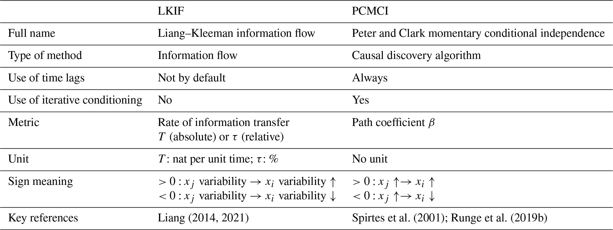
Before investigating results from the two causal methods, it is important to highlight the main differences between the two methods, which are summarized in Table 1. LKIF is directly derived from the propagation of information entropy (Liang, 2016) and quantifies the rate of information transfer from one variable to the other (Liang, 2014, 2021). PCMCI, on the other hand, is a causal network algorithm starting with a fully connected graph from which non-causal links are iteratively removed based on conditioning sets of growing cardinality (Spirtes et al., 2001; Runge et al., 2019b). The actual underlying PCMCI measure for directional statistical dependence is partial correlations, including the effect of possible causal parents. LKIF does not systematically test the latter but uses a different approach, in which the statistical dependence is measured via the information flowing from one variable to the other.
The metric used by LKIF is the rate of information transfer from variable xj to variable xi and can be expressed either in natural unit of information (nat) per unit time (for T; Eq. 5) or in percent (for τ; Eq. 6). For PCMCI, the path coefficient β (Eq. 8) measures the expected change in xi at time t (in units of standard deviation) if xj is perturbed at time t−l by 1 standard deviation. While time lags must be incorporated with PCMCI, LKIF has not been designed to work with such lags by default, although they can be used in principle (Liang et al., 2021). To this end, we can shift in time the time series of the leading variable and recompute LKIF based on the lagged time series.
While for both methods the strength of the metric, in absolute value, indicates how strongly two variables are causally linked (i.e., the larger and , the larger the causal link), the sign has a different meaning. For LKIF, a positive (negative) value of τj→i means that the variability of the source xj increases (decreases) the variability of the target xi. For PCMCI, the sign of βj→i is closely linked to the correlation between xj and xi (i.e., a positive (negative) value means that an increase in xj leads to an increase (a decrease) in xi in the subsequent time step).
Liang (2014, 2021)Spirtes et al. (2001); Runge et al. (2019b)Table 1Main differences between the two causal methods used in this study.
3.4 Comparison diagnostics
Since correct causal links are known for the three first artificial models (2D, 6D, and 9D models), we can check the performance of the two causal methods, as well as the correlation coefficient, in identifying the ground truth. The diagnostics presented here are not computed for the Lorenz (1963) model and the real-world case study, as no exact solution exists for these two cases. We compute true-positive, true-negative, false-positive, and false-negative rates. The true-positive rate is the percentage of causal links correctly detected by the method among the total number of ground truth causal links. The true-negative rate is the percentage of non-causal links correctly detected by the method among the total number of ground truth non-causal links. The false-positive rate represents the percentage of cases where the method incorrectly detects a causal link among the total number of ground truth non-causal links. The false-negative rate represents the percentage of cases where the method fails to find an existing causal link among the total number of ground truth causal links.
To summarize the results from the confusion matrix, we also compute the ϕ coefficient based on true positives (denoted TP), true negatives (denoted TN), false positives (denoted FP), and false negatives (denoted FN):
The denominator is set to 1 if any of the four sums in the denominator is equal to 0, in which case ϕ=0. A value of 1 represents a perfect prediction of ground truth causal and non-causal links by the method, while a value of 0 means that the result is not better than a random prediction. These diagnostics are presented in Table 2 and discussed in Sect. 5.1.
We provide results from the four artificial models and the real-world case study hereafter. Table 2 provides a summary of results for the three first models and will be discussed in Sect. 5.1.
4.1 2D model
For the 2D model, the numerical value of the correlation between x1 and x2 is significantly positive (R=0.23; Fig. 1a) and is similar to the analytical value (Fig. 1d), but it does not provide any indication on the direction of influence.
LKIF can accurately retrieve the correct causal link, i.e., from x2 to x1, as well as the absence of influence in the reverse direction (Fig. 1b), as was already demonstrated in Liang (2014). In addition, the numerical estimate of the rate of information transfer (; Fig. 1b) is very close to the analytical solution (; Fig. 1e), which provides confidence in the LKIF results found for this simple system.
PCMCI only captures the self-influences of x1 and x2 but is not able to capture any significant causal influence between x1 and x2 with the original time step (i.e., Δt=0.001) (Fig. 1c). This missed detection is partly due to the fact that PCMCI responds better for discrete maps with finite time steps. Indeed, the time step for discretization is too small, and if we recompute causal links with PCMCI taking every 100 time steps (Δt=0.1), we can recover the influence from x2 to x1, although the value of β is relatively small (Fig. 1c).
This example shows that LKIF performs well for such a very simple 2D system, while PCMCI struggles with the original time step. In particular, the serial dependency in this particular model might overcast the mutual dependency for a “typical” maximum lag considered by PCMCI, which has not been designed for such conditions.
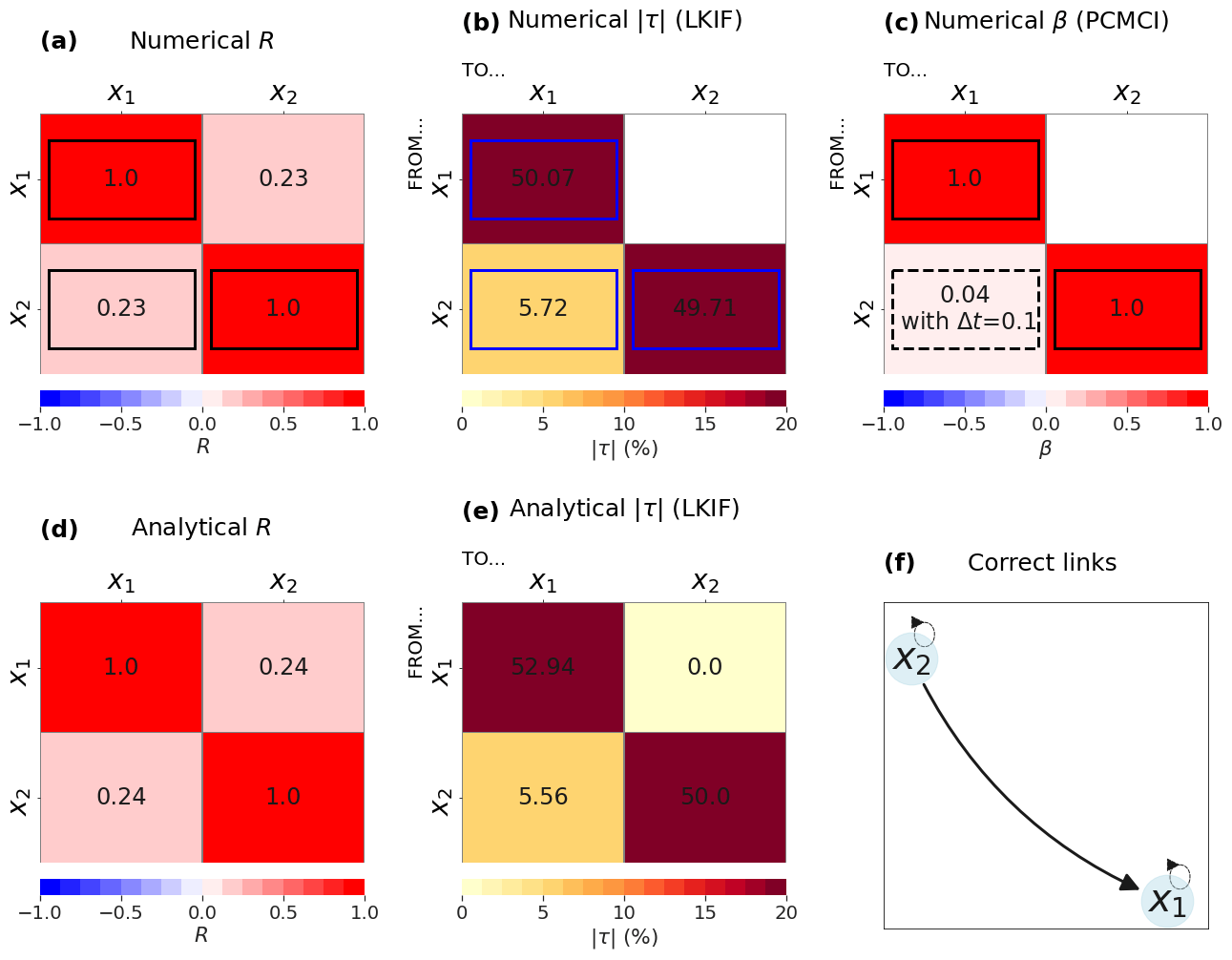
Figure 1Numerical results from the 2D model: (a) correlation coefficient, (b) rate of information transfer (LKIF, absolute value), and (c) maximum path coefficient (PCMCI) when using three lags (zero to two time steps). Analytical values of (d) correlation coefficient and (e) rate of information transfer (LKIF). (f) Correct causal links from Eq. (1). For numerical results, only significant values at the α=5 % level are shown, and correct causal links are highlighted by black or blue contours. The dashed contour in panel (c) indicates a significant value with a larger time step (Δt=0.1), while it is not significant with the original time step (Δt=0.001).
4.2 6D model
For the 6D model, the correlations are significant for all 30 pairs of variables (excluding autocorrelations), despite relatively small values for many of them (Fig. 2a). This shows that a simple correlation analysis fails to only identify the seven causal links that should be identified in this system (Fig. 2d). The largest correlation of all pairs is between x2 and x5 (R=0.37), but no causal link should exist between the two variables (i.e., this is a false positive). This large correlation probably appears because x6 influences both x2 and x5 by construction (Fig. 2d) and is thus a confounding variable. Correlations larger than 0.3 in absolute value appear for the two pairs x6–x2 and x6–x5 (Fig. 2a), which confirms the role of x6 as a confounding variable, but these correlations do not indicate the direction of influences.
Both LKIF (Fig. 2b; no lag is used) and PCMCI (Fig. 2c; use of four time lags) can capture the seven correct causal links (Fig. 2d), i.e., the directed cycle , the two-way causal link between x4 and x5, and the influence of x6 on both x2 and x5. Results from PCMCI in terms of self-influences are more accurate based on Eq. (2), as it provides two significant self-influences, i.e., x4 and x6, while LKIF identifies all six self-influences as significant. The latter result indicates that the LKIF method may fail at representing the correct self-influences, while PCMCI does not.
This example shows the strength of causal methods, which can capture the correct causal influences, while the correlation is not able to provide such information and cannot identify confounding variables and the direction of causality.
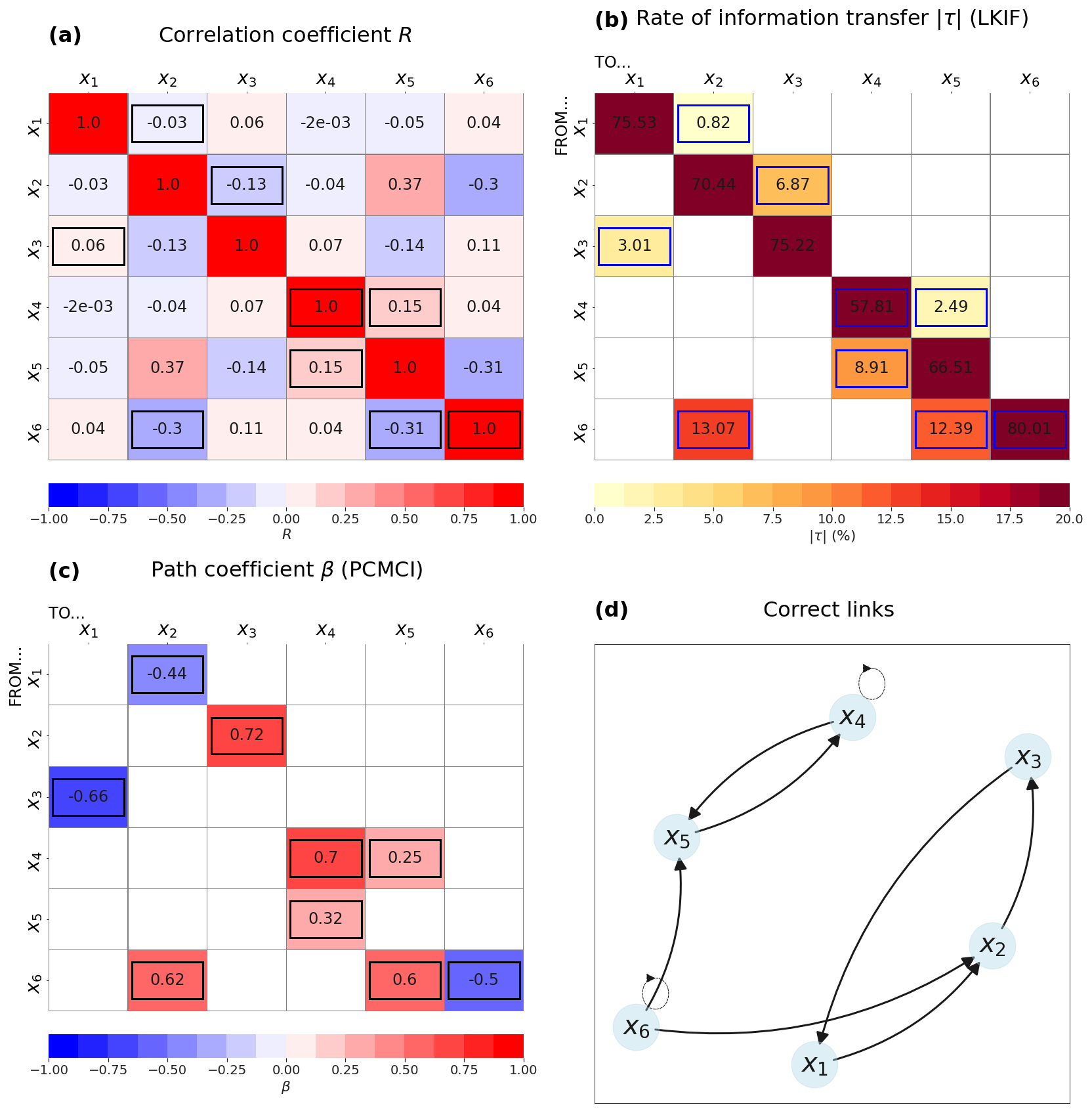
Figure 2Results from the 6D model: (a) correlation coefficient, (b) rate of information transfer (LKIF, absolute value), and (c) maximum path coefficient (PCMCI) when using four lags (zero to three time steps). (d) Correct causal links from Eq. (2). Only significant values at the α=5 % level are shown, and correct causal links are highlighted by black or blue contours.
4.3 9D model
For the 9D model, the correlation does a poor job at identifying correct causal influences (Fig. 3a). In particular, the largest correlation is between x8 and x9, which is not a correct causal link by construction (Eq. 3). As for the 6D model, this is due to the fact that x7 should influence both variables (Fig. 4d). x7 is indeed significantly correlated to both x8 and x9, but the causal direction is not identified by the correlation analysis.
Using LKIF without any lag shows that the method can detect all correct links, except x5→x4, although only four causal influences have a rate of information transfer larger than 1 % (Fig. 3b). These four influences are the ones that should appear at lag −1 (Fig. 4d, i.e., x1→x3, x6→x4, x7→x8, and x7→x9. The method also wrongly identifies 13 causal influences, even if values of information transfer remain small.
The use of time lags up to l=3 time steps with LKIF (we use 9 variables × 4 lags =36 variables in total) allows us to improve results (Fig. 4b, where the maximum value of all lags is plotted). In particular, all nine correct causal links can now be identified with , except the influence of x3 on x1, which is significant but has a much smaller value (). Five additional causal influences are wrongly identified by the method with lags up to 3 time steps, but with relatively small values ().
Using PCMCI with lags up to l=4 time steps also allows us to correctly reproduce all causal links, except that it wrongly identifies four additional causal influences but with very small values (Fig. 4c). All self-influences are also correctly identified by the two methods.
This example also demonstrates the power of causal methods compared to a correlation analysis when using an appropriate number of lags: all expected links are correctly identified. Although some wrong causal links are identified by both methods, the strength of the relationship remains small for these wrong influences.
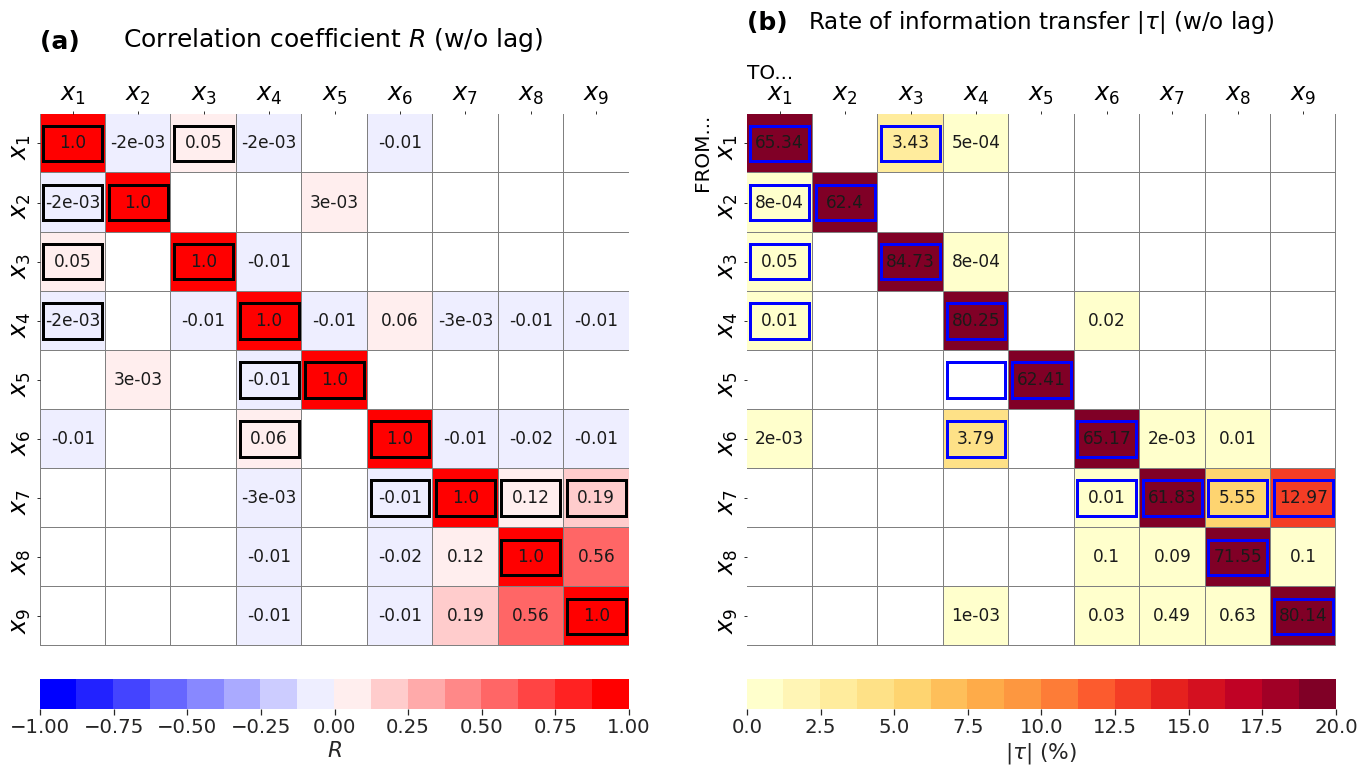
Figure 3Results from the 9D model without lags: (a) correlation coefficient and (b) rate of information transfer (LKIF, absolute value). Only significant values at the α=5 % level are shown, and correct causal links are highlighted by black or blue contours.
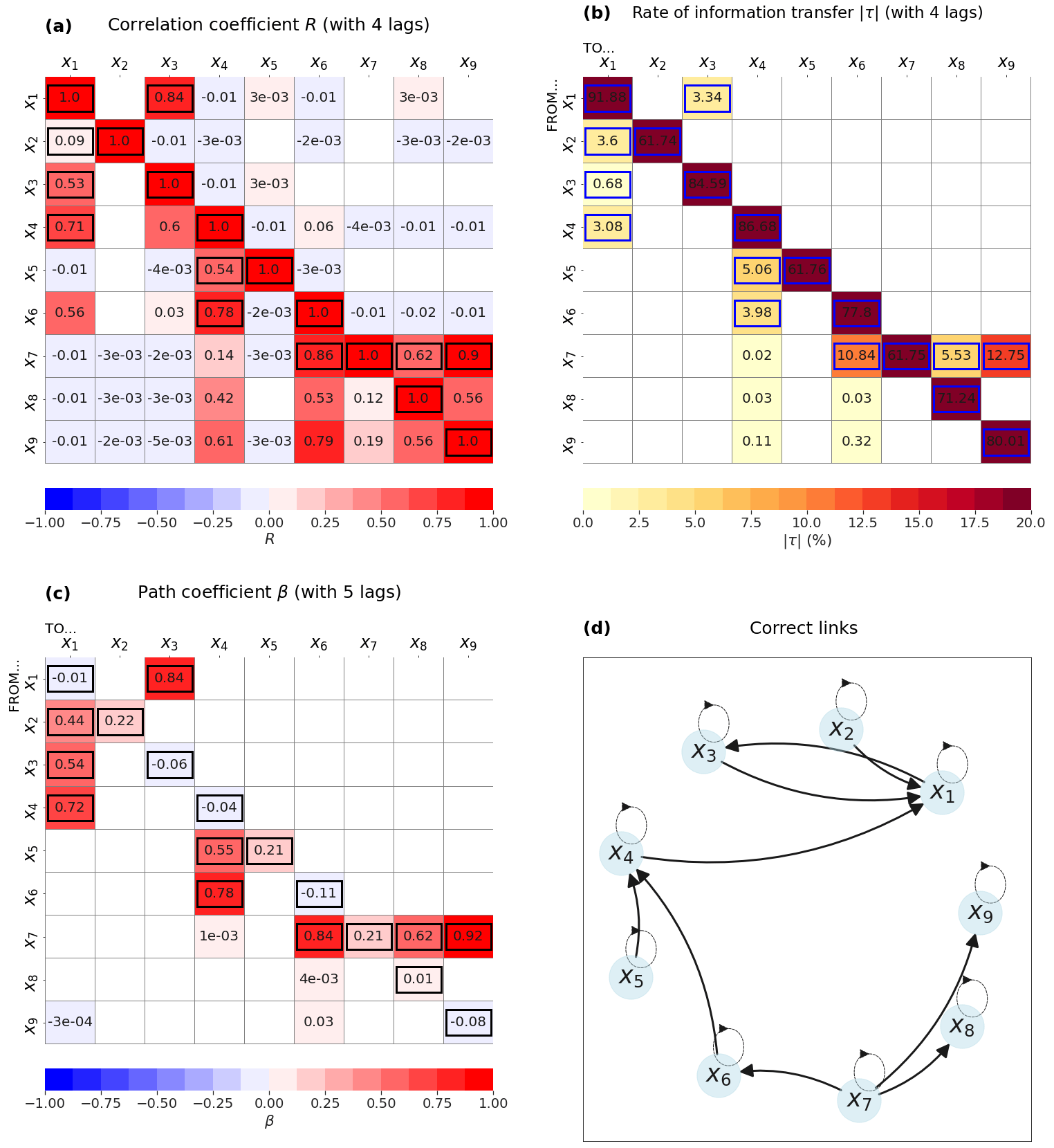
Figure 4Results from the 9D model with lags: (a) maximum correlation coefficient when using four lags (zero to three time steps), (b) maximum rate of information transfer (LKIF, absolute value) when using four lags (zero to three time steps), and (c) maximum path coefficient (PCMCI) using five lags (zero to four time steps). (d) Correct causal links from Eq. (3). Only significant values at the α=5 % level are shown, and correct causal links are highlighted by black or blue contours.
4.4 Lorenz (1963) model
The only large correlation (excluding autocorrelation) in this system is between x and y, with R=0.88 (Fig. 5a). The other correlations are very small () but significant, probably due to the length of the time series.
According to LKIF, a two-way causal link appears between x and y (Fig. 5b). This causal link is also identified by PCMCI with lags up to l=3 time steps (Fig. 5c). PCMCI also identifies a significant two-way causal link between y and z, but the value is very close to 0.
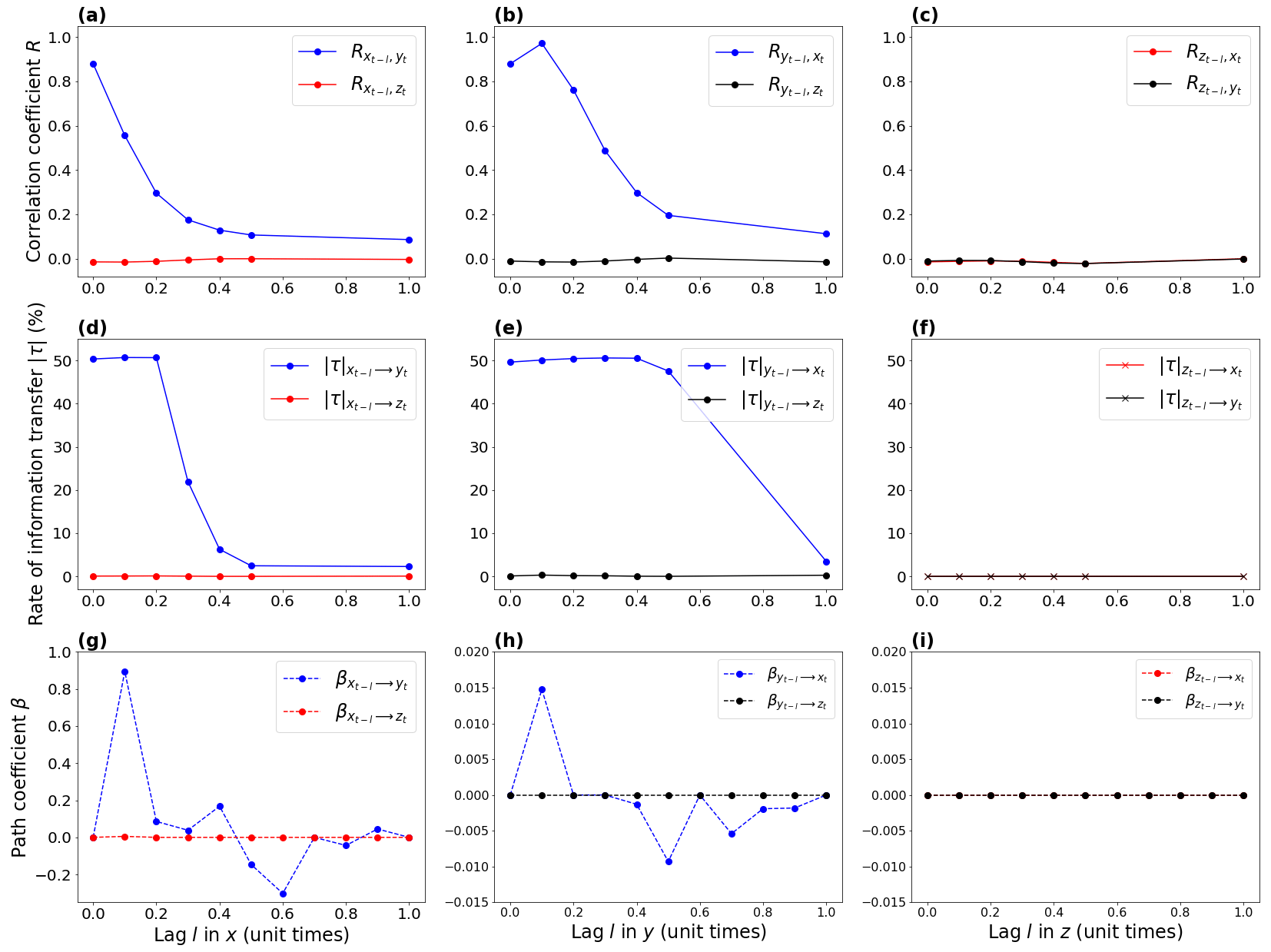
Then, we investigate whether there is a lag dependence on the results. For the correlation and LKIF, we repeat the computation by shifting the three variables one by one with a lag from 0 to 1 unit time (100 time steps) with 0.1 unit time increment (i.e., every 10 time steps). For example, we take xt−l at lag 1 unit time and keep yt and zt at lag 0, and we recompute the correlation and relative rate of information transfer. Then, we take xt−l at lag l = 0.2 unit time, keeping yt and zt at lag 0 and so on until lag l = 1 unit time. We do the same when y leads x and z and when z drives x and y. For PCMCI, all lags from 0 to 1 unit time with 0.01 unit time increment (i.e., every time step) are included in the same computation as the method is designed to work with multiple lags by default. Results are presented in Fig. 6.
The correlation coefficient between x and y decreases exponentially with increasing lag when x leads y (Fig. 6a), and it first increases from l=0 to l=0.1 unit time before decreasing exponentially when y leads x (Fig. 6b). No correlation appears between z and any of the two other variables at any lag (Fig. 6a–c).
The LKIF rates of information transfer from x to y and from y to x also decrease with increasing lag between 0 and 1 unit time, but starting with a plateau of (Fig. 6d–e). This plateau lasts from l=0 to l=0.2 unit time for (Fig. 6d) and from l=0 to l=0.4 unit time for (Fig. 6e). No information transfer exists between z and the two other variables at any lag (Fig. 6d–f), in agreement with the absence of correlation (Fig. 6a–c).
The PCMCI path coefficients between x and y also generally decrease (in the two directions) with increasing lag, although the decrease presents more variability than the correlation and LKIF, with β=0 at lag 0, the largest β value when l=0.1 unit time, and then an oscillatory behavior until l=1 unit time (Fig. 6g–h). As for the correlation and LKIF, no causal influence is found between z and the two other variables at any lag (Fig. 6g–i).
If we replace x by x2 to take nonlinearities into account and look at the triplet (x2, y, z), a strong positive correlation now appears between x2 and z (R=0.65; Fig. 5d). In addition, a strong two-way causal link now appears between x2 and z with both LKIF ( in the two directions; Fig. 5e) and PCMCI ( in the two directions; Fig. 5f). This shows that the linear versions of LKIF and PCMCI can detect causal links between nonlinear transformed variables in nonlinear models. In this case, the correlation between x and y, combined with the nonlinear forcing product xy in the third equation of the Lorenz (1963) model (z equation; Eq. 4), results in a linear correlation between z and the nonlinear non-invertible variable change x2.
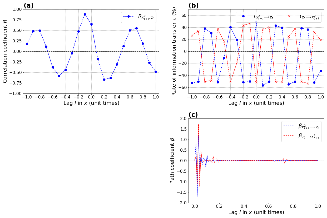
The correlation between and zt oscillates between (l=0.2 unit time) and R∼0.9 (1 unit time) with a period of ∼0.7 unit time (Fig. 7a). The rates of information transfer from to zt and from zt to also show an oscillatory behavior with a period of ∼0.35 unit time (Fig. 7b), i.e., half of the correlation oscillation. PCMCI does not exhibit such an oscillatory behavior but rather a quickly decreasing β value for small lags (Fig. 7c).
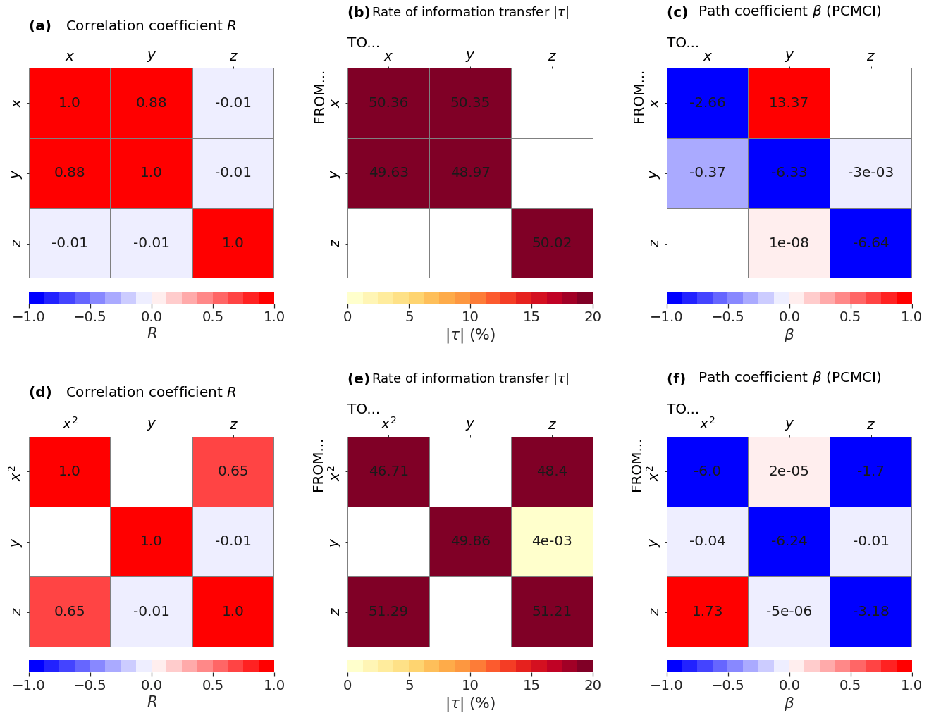
Figure 5Results from the Lorenz (1963) model when using (x, y, z): (a) correlation coefficient, (b) rate of information transfer (LKIF, absolute value), and (c) maximum path coefficient (PCMCI) when using four lags (zero to three time steps). Results from the Lorenz (1963) model when using (x2, y, z): (d) correlation coefficient, (e) rate of information transfer (LKIF, absolute value), and (c) maximum path coefficient (PCMCI) when using four lags (zero to three time steps). Only significant values at the α=5 % level are shown.
4.5 Climate indices
The real-world case study with climate indices shows that 54 % of the pairs of variables (excluding autocorrelations) are related by significant correlations when considering no lag (Fig. 8a). However, it is obvious that a large number of these pairs are correlated but not causally linked. The use of causal methods allows us to remove such spurious links, as demonstrated by the application of LKIF without any lag (Fig. 8b) and PCMCI with lags up to l = 2 months (Fig. 8c).
Results from the two causal methods present several similarities, including the AO influence on both PDO and TNA (Fig. 8b–c). Another similarity is the two-way causal link between AMO and TNA, in agreement with Vannitsem and Liang (2022) and Silini et al. (2022). The AMO–TNA influence is not surprising as both indices are computed from SST anomalies in the North Atlantic, with AMO spanning the majority of the North Atlantic and TNA focusing on the tropical region. Values of the AMO–TNA influence in the two directions are relatively strong for LKIF ( and ) compared to other pairs of influence (Fig. 8b). In addition, ENSO influences PDO according to both methods (Fig. 8b–c), and the positive sign of the correlation means that a warm Niño3.4 phase results in a positive PDO (Fig. 8a). The ENSO influence on PDO was recently reported by Vannitsem and Liang (2022), also using LKIF, and Silini et al. (2022), based on the pseudo-transfer entropy. Spatial patterns of ENSO and PDO are very similar, and PDO is often being viewed as an ENSO-like interdecadal climate variability, with PDO occurring at decadal timescales, while ENSO is predominantly an interannual phenomenon (Mantua et al., 1997; Zhang et al., 1997).
In terms of differences between the two causal methods, LKIF identifies additional causal influences of AO on PNA, NAO, and AMO, while PCMCI does not identify these causal links (Fig. 8b–c). It is well known that there is a clear relationship between AO and NAO (Deser, 2000) and that NAO is often referred to as the local manifestation of the AO (Hamouda et al., 2021). Also, according to LKIF, there are two-way causal influences between ENSO and PNA and between ENSO and TNA, which do not appear with PCMCI with lags up to l = 2 months (Fig. 8b–c). It is well known that ENSO has a major influence on the extratropical Northern Hemisphere climate variability, in particular on PNA (Horel and Wallace, 1981). However, the influence of ENSO on PNA is complicated by the fact that other mechanisms can affect this relationship, such as the position of the Pacific jet stream (Soulard et al., 2019). Our results with LKIF suggest that PNA has a stronger influence on ENSO than the reverse, which would go in favor of more complex mechanisms in action. Finally, the influence of ENSO on TNA has also been reported in the literature, and different mechanisms have been proposed (García-Serrano et al., 2017). It is interesting to find that the influence of TNA on ENSO is stronger than the reverse influence with LKIF (Fig. 8b).
The use of 12 time lags (0 to 11 months) with both methods (bringing 8 variables ×12 lags =96 variables in total for LKIF) provides additional insights (Figs. 9–10). PNA influences ENSO with a 1-month lag with LKIF (Fig. 9a) and with a 4-month lag with PCMCI (Fig. 10a). Additionally, PNA influences PDO with a 4-month lag and AMO with a 11-month lag using LKIF (Fig. 9a). However, all PNA influences appear relatively weak in intensity ( with LKIF and ).
NAO influences PDO with both methods but with very different lags depending on the method, i.e., 11 months with LKIF (Fig. 9b) and 1 month with PCMCI (Fig. 10b). It also influences TNA with LKIF with a 1-month lag. As for PNA, all significant NAO influences remain limited in intensity ( with LKIF and ).
AO is by far the climate index that influences most variables with LKIF (Fig. 9c), in agreement with Vannitsem and Liang (2022). When considering no lag, AO influences all other indices, except QBO and ENSO (Fig. 9c). The largest value of rate of information transfer is from AO to NAO with , in agreement with the value considering no lag (Fig. 8b). AO also influences TNA and AMO at larger lags with LKIF (l=1, 2, and 4 months for TNA and l = 2, 5, and 11 months for AMO). With PCMCI, AO only influences TNA at lags l = 1 to 4 months, PDO at lag l = 1 month, and QBO at lag l = 4 months (Fig. 10c). It is intriguing to notice that no AO influence on NAO appears with PCMCI.
QBO does not have any influence on any other climate indices with any of the methods (Figs. 9d and 10d).
The AMO–TNA two-way causal influence already identified in Fig. 8 also appears in the lagged plots but with contrasting behaviors depending on the causal method. With LKIF, AMO only influences TNA at lag 0 (Fig. 9e) and TNA influences AMO at lags l = 0 and 11 months (Fig. 9g). With PCMCI, the AMO influence on TNA increases with increasing lag from l = 0 to 6 months, then decreases and stays relatively constant until l = 11 months (Fig. 10e), and TNA influences AMO at lags l = 2, 4–6, 8, and 10–11 months (Fig. 10g). TNA has additional influences with PCMCI at lags l≥ 2 months (on NAO, QBO, PDO, and ENSO; Fig. 10g) and with LKIF at lags l≥ 9 months (on PDO and ENSO). The TNA influences on PDO and ENSO, appearing for both causal methods, remain limited to large lags (Figs. 9g–10g).
PDO has an influence on PNA with LKIF at lag l=6 months (Fig. 9f), which is consistent with Simon et al. (2022) using sensitivity experiments with a coupled model. According to PCMCI, PDO influences ENSO at lags l≥ 3 months (Fig. 10f).
Finally, ENSO influences PDO at lags and 6 months, and influences TNA at lags l=2 and 6 months with LKIF (Fig. 9h). With PCMCI, ENSO is the climate index that influences most variables (all but NAO), especially PDO from l=2 to 10 months, TNA from l=3 to 11 months, and AMO from l=4 to 11 months (Fig. 10h). The large role of ENSO was also reported using pseudo-transfer entropy using lags l=1 to 9 months (Silini et al., 2022).
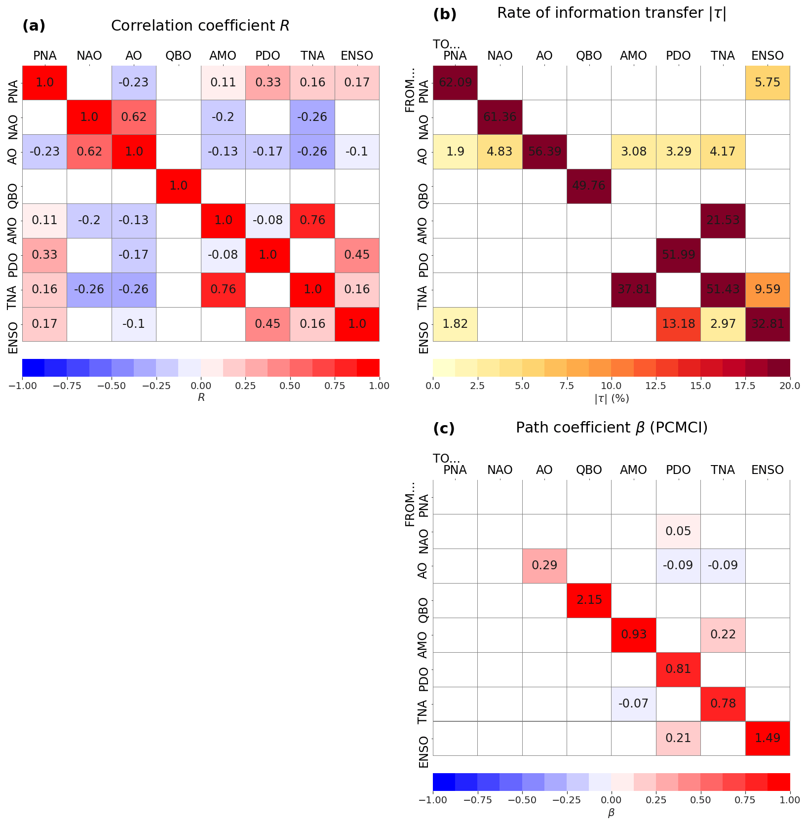
Figure 8Results from the real-world case study: (a) correlation coefficient, (b) rate of information transfer (LKIF, absolute value), and (c) maximum path coefficient (PCMCI) when using three lags (0 to 2 months). Only significant values at the α=5 % level are shown.
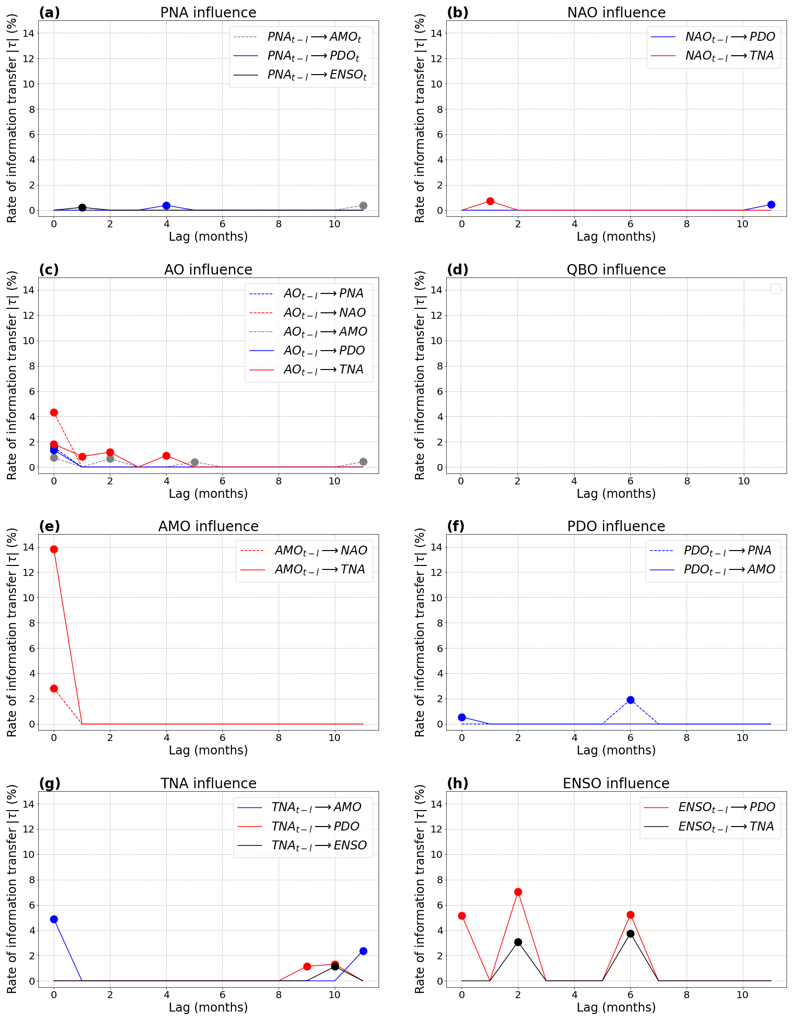
Figure 9Results from the real-world case study with LKIF (rate of information transfer; absolute value) as a function of the lag: (a) PNA influence on the other variables; (b) NAO influence; (c) AO influence; (d) QBO influence; (e) AMO influence; (f) PDO influence; (g) TNA influence; (h) ENSO influence. Only significant influences at the α=5 % level are shown as filled dots.
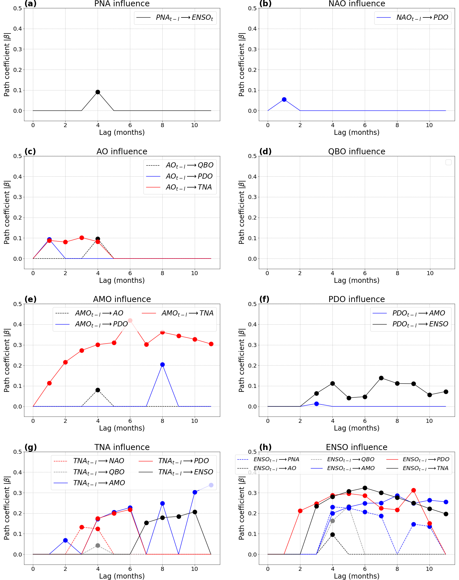
Figure 10Results from the real-world case study with PCMCI (path coefficient; absolute value) as a function of the lag: (a) PNA influence on the other variables; (b) NAO influence; (c) AO influence; (d) QBO influence; (e) AMO influence; (f) PDO influence; (g) TNA influence; (h) ENSO influence. Only significant influences at the α=5 % level are shown as filled dots.
Correlation is often used by the climate community to identify potential relationships between variables, but a statistically significant correlation does not necessarily imply causation. In our study, we used two causal methods, LKIF and PCMCI, to disentangle true causal links from spurious correlations, and we applied them to four artificial models and one real-world case study based on climate indices. Below we discuss our results compared to previous literature (Sect. 5.1 for the artificial models and Sect. 5.2 for the real-world case study).
5.1 Artificial models
For the simplest (2D) model used here, we show that LKIF can accurately reproduce the correct causal link, with relatively high accuracy compared to the analytical solution, while PCMCI fails to reproduce this link when using the original time step (Sect. 4.1 and Fig. 1). PCMCI provides the correct influence for the 2D model when taking every 100 time steps (although the β value is small), which shows that PCMCI responds better for discrete maps with finite time steps. For the 6D model, both LKIF and PCMCI can detect the correct causal links (Sect. 4.2 and Fig. 2). For the 9D nonlinear model, PCMCI allows us to retrieve the correct causal relationships, while some care with the number of lags is needed with LKIF to achieve appropriate results (Sect. 4.3 and Figs. 3–4). This shows that LKIF performs better for simpler systems and presents a few more difficulties with more complex models with several lags. On the other hand, PCMCI does not work well in the presence of very strong autocorrelations but may be preferential over LKIF as the number of variables increases. Results from the Lorenz (1963) model are more complicated to interpret as the system is highly nonlinear and chaotic. Both methods detect the same causal links (Sect. 4.4 and Fig. 5), although some differences appear in the dependence of the causal influence on the time lag (Figs. 6–7). Moreover, the combination of model nonlinearities and nonlinear variable changes can result in linear causal links detectable by LKIF and PCMCI (Fig. 5).
The above results are not entirely comparable to findings from Krakovská et al. (2018) from a methodological perspective, as the latter used other causal methods and different coupled systems. However, a similarity is the fact that some methods (Granger causality and its extensions) better perform with the simplest models, while other methods (CCM and predictability improvement) are better suited for more complex systems (Krakovská et al., 2018). This goes in hand with LKIF being better with the specific time-continuous 2D model studied here, while PCMCI is well suited for the time-discrete 9D model of our analysis. Thus, the key finding from Krakovská et al. (2018), that “it is important to choose the right method for a particular type of data”, is also valid for our study.
The main novelties compared to Krakovská et al. (2018) are that (1) we use two causal methods that have not been compared yet, (2) we compare our causal methods to the classical correlation coefficient, (3) we assess causality between nonlinear variable changes, and (4) we apply the two methods to a real-world case study. Regarding (1), no definite conclusion can be provided as to which method is the best: it depends on the system used. For certain very simple models, LKIF appears to be preferential over PCMCI, although PCMCI has not been designed for the particular 2D model used here (Sect. 4.1). For a more complex model involving more variables and several lags, like the 9D model, PCMCI may be better suited. In any case, we recommend to use as many methods as possible for a specific problem to increase the robustness of results. Regarding (2), we show that both LKIF and PCMCI are superior to correlation, as they allow us to remove spurious links. Regarding (3), we show that the combination of model nonlinearities with nonlinear variable changes can result in linear causal links, detectable by both LKIF or PCMCI. Point (4) is discussed in Sect. 5.2.
Table 2True-positive, true-negative, false-positive, and false-negative rates (in %), as well as ϕ coefficient, for the correlation and the two causal methods (LKIF and PCMCI) for the first three artificial models (2D, 6D, and 9D models, the latter without and with lags), excluding self-influences. The number of ground truth correct (incorrect) links (without considering if the exact time lags are reproduced or not) is indicated in parentheses after “True positives” (“True negatives”) for each model. For the 2D model and PCMCI, numbers are also provided in parentheses for the case with larger sampling time step (Δt=0.1).
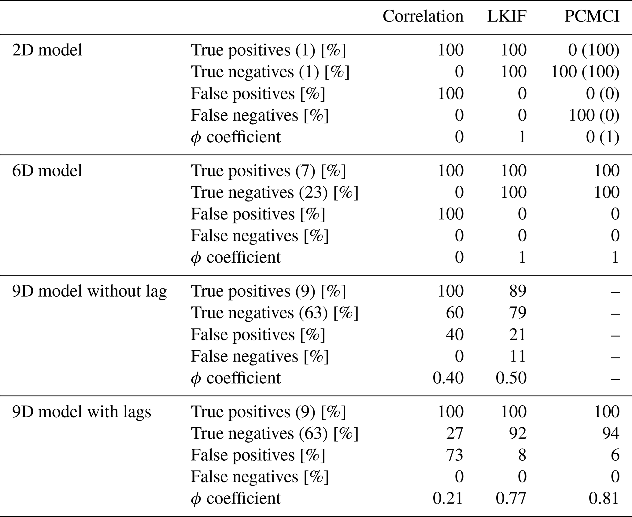
Table 2 provides true-positive, true-negative, false-positive, and false-negative rates, as well as the ϕ coefficient, for the correlation and the two causal methods used in this study and for the three first artificial models (2D, 6D, and 9D models). For the 9D model, a distinction is made between the case where lags are not considered (PCMCI is not used in this case) and the case where lags are considered. Results show that the correlation has a large chance of detecting false positives (i.e., incorrect detection of causal influences) for all models; thus, the correlation largely overestimates causal links. LKIF and PCMCI allow us to substantially reduce false positives, with 0 % for the 2D and 6D models with both methods, 21 % for the 9D model without lag with LKIF, and <10 % for the 9D model with lags with both methods. For the 2D model, LKIF perfectly reproduces the right causal links (ϕ=1), while the correlation coefficient and PCMCI (with the original time step) do not make better than a random prediction (ϕ=0). Only when using a larger sampling time step can PCMCI reproduce the correct causal links. For the 6D model, both LKIF and PCMCI accurately reproduce the ground truth (ϕ=1), while the correlation coefficient again does not make better than a random prediction and identifies all relationships as causal (ϕ=0 and false-positive rate =100 %). For the 9D model without lag (PCMCI not included), the correlation does a better job at identifying a certain amount of true negatives (60 %) compared to the 2D and 6D models, but LKIF provides overall better results (ϕ=0.5 for LKIF vs. ϕ=0.4 for correlation), despite the identification of one false negative with LKIF (Fig. 3b). For the 9D model with lags, the performance of the two causal methods is clearly better than the correlation (ϕ=0.21), with PCMCI (ϕ=0.81) performing slightly better than LKIF (ϕ=0.77).
5.2 Climate indices
In our study, we extend previous analyses from Vannitsem and Liang (2022) and Silini et al. (2022) by using monthly time series of climate indices in the Atlantic and Pacific regions. We use the same seven climate indices as Vannitsem and Liang (2022); add QBO to the list to have four indices characterizing both the atmosphere and ocean; and do not use local air temperature, precipitation, or insolation. Vannitsem and Liang (2022) also computed LKIF based on these indices but focused on the dependence of the rate of information transfer on the timescale (using a time-moving window) and did not compare LKIF to another method. Silini et al. (2022) also used NAO, QBO, AMO, PDO, and ENSO (Niño3.4); they used a slightly different index for TNA, and they incorporated seven additional indices. The causal method used by Silini et al. (2022) is the pseudo-transfer entropy method (Silini and Masoller, 2021).
Due to the small methodological differences in our analysis compared to Vannitsem and Liang (2022) (see above), some small differences appear, but key results with LKIF remain similar. In particular, we find that AO is the largest driver of all variables as it influences all other indices, except QBO and ENSO (Sect. 4.5 and Fig. 8b). We show that the AO influence mainly occurs at lag l=0 (Fig. 9c). This is in agreement with Vannitsem and Liang (2022), who find that AO plays a key role at short timescale. PCMCI only identifies two AO influences with lags shorter than 2 months, i.e., to PDO and TNA (Fig. 10c). It is particularly intriguing to see that PCMCI does not detect the AO influence on NAO (Fig. 8c), while LKIF does (Fig. 8b), as NAO is often referred to as the local manifestation of AO (Hamouda et al., 2021). This discrepancy might hide seasonal differences, as for example winter and summer NAO have different spatial patterns (Folland et al., 2009).
ENSO has a relatively large influence on other climate indices, especially on PDO for both LKIF and PCMCI (Fig. 8b–c). The pivotal role of ENSO was already identified by Silini et al. (2022) and is not surprising due to its importance on the global climate (Timmermann et al., 2018). ENSO has a clear influence on PDO at lags 2 to 10 months for PCMCI (Fig. 10h), while it only appears at lags 0, 2 and 6 months for LKIF (Fig. 9h). This ENSO–PDO influence was detected from lags 1 to 7 with pseudo-transfer entropy (Silini et al., 2022), thus somewhere in between PCMCI and LKIF. The other clear ENSO influence according to PCMCI, LKIF and pseudo-transfer entropy is on TNA, at lags 2 and 6 months with LKIF (Fig. 9h), at lags 3–11 months with PCMCI (Fig. 10h), and at lags 1–9 months with pseudo-transfer entropy (Silini et al., 2022). According to PCMCI and pseudo-transfer entropy, ENSO also largely influences other climate indices than PDO and TNA at different lags, which is not the case for LKIF. More research would be needed to further investigate this difference between causal methods.
In this study, we compare two independent causal methods, namely, the Liang–Kleeman information flow (LKIF) and the Peter and Clark momentary conditional independence (PCMCI), and the Pearson correlation coefficient. We use five different datasets with an increasing level of complexity, including three stochastic models, one nonlinear deterministic model, and one real-world case study.
We show that both causal methods are superior to the correlation, which suffers from five key limitations: random coincidence, no identification of the direction of causality, external drivers not distinguished from direct drivers, no identification of potential nonlinear influences, and application to bivariate cases only. For most models and the real-world case study, the number of significant correlations is much larger than the number of significant causal links, which is incorrect from a causal perspective for the three first models. By extension, we assume that the correlation also suffers from this overestimation in the real-world case study, and causal methods allow us to improve results.
When comparing both causal methods together, LKIF can accurately reproduce the correct causal link in the 2D model, while PCMCI cannot with the original time step and needs to be computed with a larger sampling time step to provide correct causal links, although the influence remains small. For the 6D model, both methods can capture the seven correct causal links. For the 9D model, PCMCI correctly reproduces all causal links, and LKIF without any time lag is not totally accurate. When used with time lags, LKIF can identify the correct causal links.
For the Lorenz (1963) model, results are more complicated to interpret as the system is time-continuous, nonlinear, and chaotic. Both causal methods show a strong two-way causal link between x and y, while no causal link appears between z and the two other variables. However, when we replace x by x2 to take nonlinearities into account, x2 and z are causally linked (in the two directions) with both methods. We also show that both LKIF and PCMCI display a decrease in the two-way causal influence between x and y with increasing time lag, although the shape of this decrease is different between methods. Additionally, the oscillatory behavior in correlation coefficient and LKIF for the x2–z pair as a function of lag is not displayed by PCMCI.
Finally, the real-world case study with climate indices provides some similarities but also important differences between the two methods. In terms of similarities, AO influences both PDO and TNA, there is a two-way causal link between AMO and TNA, and ENSO influences PDO. In terms of differences, LKIF identifies additional influences of AO on PNA, NAO, and AMO, as well as two-way causal links between ENSO and PNA and between ENSO and TNA. When using 12 time lags, the number of influences detected by PCMCI becomes larger compared to LKIF, e.g., ENSO has a large influence on all other variables except NAO, while AO remains the largest influencer (at smaller lags) with LKIF. More detailed analysis of the physical processes would be needed to identify correct causal links between these climate indices.
In summary, this analysis shows that both causal methods should be preferred to correlation when it comes to identify causal links. Additionally, as both LKIF and PCMCI display strengths and weaknesses when used with relatively simple models in which correct causal links can be detected by construction, we do not recommend one or the other method but rather encourage the climate community to use several methods whenever possible. We highlight that both methods, as used here, assume linearity, so results need to be taken with caution for nonlinear problems, such as the Lorenz (1963) system and the real-world case study. The use of extensions of the methods for which fully nonlinear terms are taken into account are necessary to complement the current results (e.g., Pires et al., 2024). Also, both LKIF and PCMCI deal with direct causal links, while other methods, such as interventional causality (Baldovin et al., 2020), can detect indirect influences. Further analysis would be needed to explore this aspect. Lastly, we could test the robustness of the methods to noise and their performance in the context of high-dimensional systems.
The climate indices were retrieved from the Physical Sciences Laboratory (PSL) of the National Oceanic and Atmospheric Administration (NOAA; https://psl.noaa.gov/data/climateindices/list/, PSL, 2023). The Python scripts to produce the outputs and figures of this article, including the computation of LKIF, are available on Zenodo: https://doi.org/10.5281/zenodo.8383534 (Docquier, 2023).
DD, GDC, RVD, CALP, AS and SV designed the study. DD generated the model datasets and retrieved the climate indices. DD computed the LKIF method and Pearson correlation onto the datasets, and GDC ran the PCMCI algorithm. DD led the writing of the manuscript, with contributions from all co-authors. DD created all figures, with the help of GDC. All authors participated to the data analysis and interpretation.
At least one of the (co-)authors is a member of the editorial board of Nonlinear Processes in Geophysics. The peer-review process was guided by an independent editor, and the authors also have no other competing interests to declare.
Publisher’s note: Copernicus Publications remains neutral with regard to jurisdictional claims made in the text, published maps, institutional affiliations, or any other geographical representation in this paper. While Copernicus Publications makes every effort to include appropriate place names, the final responsibility lies with the authors.
We thank X. San Liang for his feedback related to our analysis. We also thank the editor Stefano Pierini and two anonymous reviewers for their comments, which helped to improve our article.
David Docquier, Giorgia Di Capua, Reik Donner, Carlos Pires, Amélie Simon, and Stéphane Vannitsem were supported by ROADMAP (Role of ocean dynamics and Ocean-Atmosphere interactions in Driving cliMAte variations and future Projections of impact-relevant extreme events; https://jpi-climate.eu/project/roadmap/, last access: 21 February 2024), a coordinated JPI-Climate/JPI-Oceans project. David Docquier and Stéphane Vannitsem received funding from the Belgian Federal Science Policy Office under contract B2/20E/P1/ROADMAP. Giorgia Di Capua and Reik Donner were supported by the German Federal Ministry for Education and Research (BMBF) via the ROADMAP project (grant no. 01LP2002B). Amélie Simon and Carlos Pires were supported by Portuguese funds: Fundação para a Ciência e a Tecnologia (FCT) I.P./MCTES through national funds (PIDDAC) – UIDB/50019/2020 (https://doi.org/10.54499/UIDB/50019/2020), UIDP/50019/2020 (https://doi.org/10.54499/UIDP/50019/2020) and LA/P/0068/2020 (https://doi.org/10.54499/LA/P/0068/2020), and the project JPIOCEANS/0001/2019 (ROADMAP).
This paper was edited by Stefano Pierini and reviewed by two anonymous referees.
Årthun, M., Eldevik, T., Smedsrud, L. H., Skagseth, Ø., and Ingvaldsen, R. B.: Quantifying the influence of Atlantic heat on Barents Sea ice variability and retreat, J. Climate, 25, 4736–4743, https://doi.org/10.1175/JCLI-D-11-00466.1, 2012. a
Bach, E., Motesharrei, S., Kalnay, E., and Ruiz-Barradas, A.: Local atmosphere-ocean predictability: Dynamical origins, lead times, and seasonality, J. Climate, 32, 7507–7519, https://doi.org/10.1175/JCLI-D-18-0817.1, 2019. a
Baldovin, M., Cecconi, F., and Vulpiani, A.: Understanding causation via correlations and linear response theory, Phys. Rev. Res., 2, 043436, https://doi.org/10.1103/PhysRevResearch.2.043436, 2020. a, b
Benjamini, Y. and Hochberg, Y.: Controlling the False Discovery Rate: A practical and powerful approach to multiple testing, J. Roy. Stat. Soc. B, 57, 289–300, https://doi.org/10.1111/j.2517-6161.1995.tb02031.x, 1995. a
Bishop, S. P., Small, R. J., Bryan, F. O., and Tomas, R. A.: Scale dependence of midlatitude air-sea interaction, J. Climate, 30, 8207–8221, https://doi.org/10.1175/JCLI-D-17-0159.1, 2017. a
Coufal, D., Jakubík, J., Jacjay, N., Hlinka, J., Krakovská, A., and Paluš, M.: Detection of coupling delay: A problem not yet solved, Chaos, 27, 083109, https://doi.org/10.1063/1.4997757, 2017. a
Deser, C.: On the teleconnectivity of the “Arctic Oscillation”, Geophys. Res. Lett., 27, 779–782, https://doi.org/10.1029/1999GL010945, 2000. a
Di Capua, G., Kretschmer, M., Donner, R. V., van den Hurk, B., Vellore, R., Krishnan, R., and Coumou, D.: Tropical and mid-latitude teleconnections interacting with the Indian summer monsoon rainfall: a theory-guided causal effect network approach, Earth Syst. Dynam., 11, 17–34, https://doi.org/10.5194/esd-11-17-2020, 2020a. a
Di Capua, G., Runge, J., Donner, R. V., van den Hurk, B., Turner, A. G., Vellore, R., Krishnan, R., and Coumou, D.: Dominant patterns of interaction between the tropics and mid-latitudes in boreal summer: causal relationships and the role of timescales, Weather Clim. Dynam., 1, 519–539, https://doi.org/10.5194/wcd-1-519-2020, 2020b. a
Docquier, D.: Codes to compute Liang index and correlation for comparison study, Zenodo [code], https://doi.org/10.5281/zenodo.8383534, 2023. a
Docquier, D., Grist, J. P., Roberts, M. J., Roberts, C. D., Semmler, T., Ponsoni, L., Massonnet, F., Sidorenko, D., Sein, D. V., Iovino, D., Bellucci, A., and Fichefet, T.: Impact of model resolution on Arctic sea ice and North Atlantic Ocean heat transport, Clim. Dynam., 53, 4989–5017, https://doi.org/10.1007/s00382-019-04840-y, 2019. a
Docquier, D., Vannitsem, S., Ragone, F., Wyser, K., and Liang, X. S.: Causal links between Arctic sea ice and its potential drivers based on the rate of information transfer, Geophys. Res. Lett., 49, e2021GL095892, https://doi.org/10.1029/2021GL095892, 2022. a
Docquier, D., Vannitsem, S., and Bellucci, A.: The rate of information transfer as a measure of ocean–atmosphere interactions, Earth Syst. Dynam., 14, 577–591, https://doi.org/10.5194/esd-14-577-2023, 2023. a
Enfield, D. B., Mestas-Nuñez, A. M., Mayer, D. A., and Cid-Serrano, L.: How ubiquitous is the dipole relationship in tropical Atlantic sea surface temperatures?, J. Geophys. Res., 104, 7841–7848, https://doi.org/10.1029/1998JC900109, 1999. a
Enfield, D. B., Mestas-Nuñez, A. M., and Trimble, P. J.: The Atlantic Multidecadal Oscillation and its relation to rainfall and river flows in the continental U.S., Geophys. Res. Lett., 28, 2077–2080, https://doi.org/10.1029/2000GL012745, 2001. a
Folland, C. K., Knight, J., Linderholm, H. W., Fereday, D., Ineson, S., and Hurrell, J. W.: The summer North Atlantic Oscillation: Past, present, and future, J. Climate, 22, 1082–1103, https://doi.org/10.1175/2008JCLI2459.1, 2009. a
García-Serrano, J., Cassou, C., Douville, H., Giannini, A., and Doblas-Reyes, F. J.: Revisiting the ENSO teleconnection to the Tropical North Atlantic, J. Climate, 30, 6945–6957, https://doi.org/10.1175/JCLI-D-16-0641.1, 2017. a
Granger, C. W. J.: Investigating causal relations by econometric models and cross-spectral methods, Econometrica, 37, 424–438, https://doi.org/10.2307/1912791, 1969. a
Hagan, D. F. T., Dolman, H. A. J., Wang, G., Lim Kam Sian, K. T. C., Yang, K., Ullah, W., and Shen, R.: Contrasting ecosystem constraints on seasonal terrestrial CO2 and mean surface air temperature causality projections by the end of the 21st century, Environ. Res. Lett., 17, 124019, https://doi.org/10.1088/1748-9326/aca551, 2022. a
Hamouda, M. E., Pasquero, C., and Tziperman, E.: Decoupling of the Arctic Oscillation and North Atlantic Oscillation in a warmer climate, Nat. Clim. Change, 11, 137–142, https://doi.org/10.1038/s41558-020-00966-8, 2021. a, b
Horel, J. D. and Wallace, J. M.: Planetary-scale atmospheric phenomena associated with the Southern Oscillation, Mon. Weather Rev., 109, 813–829, https://doi.org/10.1175/1520-0493(1981)109<0813:PSAPAW>2.0.CO;2, 1981. a
Huang, Y., Franzke, C. L. E., Yuan, N., and Fu, Z.: Systematic identification of causal relations in high-dimensional chaotic systems: application to stratosphere-troposhere coupling, Clim. Dynam., 55, 2469–2481, https://doi.org/10.1007/s00382-020-05394-0, 2020. a
Jiang, S., Hu, H., Zhang, N., Lei, L., and Bai, H.: Multi-source forcing effects analysis using Liang–Kleeman information flow method and the community atmosphere model (CAM4.0), Clim. Dynam., 53, 6035–6053, https://doi.org/10.1007/s00382-019-04914-x, 2019. a
Kaplan, A., Cane, M. A., Kushnir, Y., Clement, A. C., Blumenthal, M. B., and Rajagopalan, B.: Analyses of global sea surface temperature 1856–1991, J. Geophys. Res., 103, 18567–18589, https://doi.org/10.1029/97JC01736, 1998. a
Krakovská, A. and Hanzely, F.: Testing for causality in reconstructed state spaces by an optimized mixed prediction method, Phys. Rev. E, 94, 052203, https://doi.org/10.1103/PhysRevE.94.052203, 2016. a
Krakovská, A., Jakubík, J., Chvosteková, M., Coufal, D., Jajcay, N., and Paluš, M.: Comparison of six methods for the detection of causality in a bivariate time series, Phys. Rev. E, 97, 042207, https://doi.org/10.1103/PhysRevE.97.042207, 2018. a, b, c, d, e, f
Kretschmer, M., Coumou, D., Donges, J. F., and Runge, J.: Using causal effect networks to analyze different Arctic drivers of midlatitude winter circulation, J. Climate, 29, 4069–4081, https://doi.org/10.1175/JCLI-D-15-0654.1, 2016. a
Liang, X. S.: Unraveling the cause-effect relation between time series, Phys. Rev. E, 90, 052150, https://doi.org/10.1103/PhysRevE.90.052150, 2014. a, b, c, d, e, f
Liang, X. S.: Normalizing the causality between time series, Phys. Rev. E, 92, 022126, https://doi.org/10.1103/PhysRevE.92.022126, 2015. a, b
Liang, X. S.: Information flow and causality as rigorous notions ab initio, Phys. Rev. E, 94, 052201, https://doi.org/10.1103/PhysRevE.94.052201, 2016. a, b, c, d
Liang, X. S.: Normalized multivariate time series causality analysis and causal graph reconstruction, Entropy, 23, 679, https://doi.org/10.3390/e23060679, 2021. a, b, c, d, e, f, g
Liang, X. S. and Kleeman, R.: Information transfer between dynamical system components, Phys. Rev. Lett., 95, 244101, https://doi.org/10.1103/PhysRevLett.95.244101, 2005. a, b, c
Liang, X. S., Xu, F., Rong, Y., Zhang, R., Tang, X., and Zhang, F.: El Niño Modoki can be mostly predicted more than 10 years ahead of time, Sci. Rep., 11, 17860, https://doi.org/10.1038/s41598-021-97111-y, 2021. a
Lorenz, E. N.: Deterministic nonperiodic flow, J. Atmos. Sci., 20, 130–141, https://doi.org/10.1175/1520-0469(1963)020<0130:DNF>2.0.CO;2, 1963. a, b, c, d, e, f, g, h, i, j, k, l, m, n
Manshour, P., Balasis, G., Consolini, G., Papadimitriou, C., and Paluš, M.: Causality and information transfer between the solar wind and the magnetosphere-ionosphere system, Entropy, 23, 390, https://doi.org/10.3390/e23040390, 2021. a
Mantua, N. J., Hare, S. R., Zhang, Y., Wallace, J. M., and Francis, R. C.: A Pacific interdecadal climate oscillation with impacts on salmon production, B. Am. Meteor. Soc., 78, 1069–1080, https://doi.org/10.1175/1520-0477(1997)078<1069:APICOW>2.0.CO;2, 1997. a
McGraw, M. C. and Barnes, E. A.: Memory matters: A case for Granger causality in climate variability studies, J. Climate, 31, 3289–3300, https://doi.org/10.1175/JCLI-D-17-0334.1, 2018. a
Mosedale, T. J., Stephenson, D. B., Collins, M., and Mills, T. C.: Granger causality of coupled climate processes: Ocean feedback on the North Atlantic Oscillation, J. Climate, 19, 1182–1194, https://doi.org/10.1175/JCLI3653.1, 2006. a
Paluš, M. and Vejmelka, M.: Directionality of coupling from bivariate time series: How to avoid false causalities and missed connections, Phys. Rev. E, 75, 056211, https://doi.org/10.1103/PhysRevE.75.056211, 2007. a
Paluš, M., Komárek, V., Hrnčír, Z., and Štěrbová, K.: Synchronization as adjustment of information rates: Detection from bivariate time series, Phys. Rev. E, 63, 046211, https://doi.org/10.1103/PhysRevE.63.046211, 2001. a
Paluš, M., Krakovská, A., Jakubík, J., and Chvosteková, M.: Causality, dynamical systems and the arrow of time, Chaos, 28, 075307, https://doi.org/10.1063/1.5019944, 2018. a
Pfleiderer, P., Schleussner, C.-F., Geiger, T., and Kretschmer, M.: Robust predictors for seasonal Atlantic hurricane activity identified with causal effect networks, Weather Clim. Dynam., 1, 313–324, https://doi.org/10.5194/wcd-1-313-2020, 2020. a
Physical Sciences Laboratory (PSL): Climate indices: Monthly atmospheric and ocean time series, National Oceanic and Atmospheric Administration (NOAA) [data set], https://psl.noaa.gov/data/climateindices/list/, last access: 20 January 2023. a
Pires, C., Docquier, D., and Vannitsem, S.: A general theory to estimate information transfer in nonlinear systems, Phys. D, 458, 133988, https://doi.org/10.1016/j.physd.2023.133988, 2024. a, b
Runge, J.: Causal network reconstruction from time series: From theoretical assumptions to practical estimation, Chaos, 28, 075310, https://doi.org/10.1063/1.5025050, 2018. a
Runge, J., Bathiany, S., Bollt, E., Camps-Valls, G., Coumou, D., Deyle, E., Glymour, C., Kretschmer, M., Mahecha, M. D., Munoz-Mari, J., van Nes, E. H., Peters, J., Quax, R., Reichstein, M., Scheffer, M., Scholkopf, B., Spirtes, P., Sugihara, G., Sun, J., Zhang, K., and Zscheischler, J.: Inferring causation from time series in Earth system sciences, Nat. Commun., 10, 2553, https://doi.org/10.1038/s41467-019-10105-3, 2019a. a
Runge, J., Nowack, P., Kretschmer, M., Flaxman, S., and Sejdinovic, D.: Detecting and quantifying causal associations in large nonlinear time series datasets, Sci. Adv., 5, eaau4996, https://doi.org/10.1126/sciadv.aau4996, 2019b. a, b, c, d, e
Schreiber, T.: Measuring information transfer, Phys. Rev. Lett., 85, 461–464, https://doi.org/10.1103/PhysRevLett.85.461, 2000. a
Silini, R. and Masoller, C.: Fast and effective pseudo transfer entropy for bivariate data-driven causal influences, Sci. Rep., 11, 8423, https://doi.org/10.1038/s41598-021-87818-3, 2021. a
Silini, R., Tirabassi, G., Barreiro, M., Ferranti, L., and Masoller, C.: Assessing causal dependencies in climatic indices, Clim. Dynam., 61, 79–89, https://doi.org/10.1007/s00382-022-06562-0, 2022. a, b, c, d, e, f, g, h, i, j, k
Simon, A., Gastineau, G., Frankignoul, C., Lapin, V., and Ortega, P.: Pacific Decadal Oscillation modulates the Arctic sea-ice loss influence on the midlatitude atmospheric circulation in winter, Weather Clim. Dynam., 3, 845–861, https://doi.org/10.5194/wcd-3-845-2022, 2022. a
Small, R. J., Bryan, F. O., Bishop, S. P., Larson, S., and Tomas, R. A.: What drives upper-ocean temperature variability in coupled climate models and observations, J. Climate, 33, 577–596, https://doi.org/10.1175/JCLI-D-19-0295.1, 2020. a
Soulard, N., Lin, H., and Yu, B.: The changing relationship between ENSO and its extratropical response patterns, Sci. Rep., 9, 6507, https://doi.org/10.1038/s41598-019-42922-3, 2019. a
Spirtes, P., Glymour, C., and Scheines, R.: Causation, Prediction, and Search (Second Edition), The MIT press, Boston, https://doi.org/10.7551/mitpress/1754.001.0001, 2001. a, b, c, d
Subramaniyam, N. P., Donner, R. V., Caron, D., Panuccio, G., and Hyttinen, J.: Causal coupling inference from multivariate time series based on ordinal partition transition networks, Nonlinear Dynam., 105, 555–578, https://doi.org/10.1007/s11071-021-06610-0, 2021. a
Sugihara, G., May, R., Ye, H., Hsieh, C.-H., Deyle, E., Fogarty, M., and Munch, S.: Detecting causality in complex ecosystems, Science, 338, 496–500, https://doi.org/10.1126/science.1227079, 2012. a, b
Timmermann, A., An, S.-I., Kug, J.-S., Jin, F.-F., Cai, W., Capotondi, A., Cobb, K. M., Lengaigne, M., McPhaden, M. J., Stuecker, M. F., Stein, K., Wittenberg, A. T., Yun, K.-S., Bayr, T., Chen, H.-C., Chikamoto, Y., Dewitte, B., Dommenget, D., Grothe, P., Guilyardi, E., Ham, Y.-G., Hayashi, M., Ineson, S., Kang, D., Kim, S., Kim, W., Lee, J.-Y., Li, T., Luo, J.-J., McGregor, S., Planton, Y., Power, S., Rashid, H., Ren, H.-L., Santoso, A., Takahashi, K., Todd, A., Wang, G., Wang, G., Xie, R., Yang, W.-H., Yeh, S.-W., Yoon, J., Zeller, E., and Zhang, X.: El Niño–Southern Oscillation complexity, Nature, 559, 535–545, https://doi.org/10.1038/s41586-018-0252-6, 2018. a
Tirabassi, G., Masoller, C., and Barreiro, M.: A study of the air–sea interaction in the South Atlantic Convergence Zone through Granger causality, Int. J. Climatol., 35, 3440–3453, https://doi.org/10.1002/joc.4218, 2015. a
van Nes, E. H., Scheffer, M., Brovkin, V., Lenton, T. M., Ye, H., Deyle, E., and Sugihara, G.: Causal feedbacks in climate change, Nat. Clim. Change, 5, 445–448, https://doi.org/10.1038/NCLIMATE2568, 2015. a
Vannitsem, S. and Ekelmans, P.: Causal dependences between the coupled ocean–atmosphere dynamics over the tropical Pacific, the North Pacific and the North Atlantic, Earth Syst. Dynam., 9, 1063–1083, https://doi.org/10.5194/esd-9-1063-2018, 2018. a
Vannitsem, S. and Liang, X. S.: Dynamical dependencies at monthly and interannual time scales in the climate system: Study of the North Pacific and Atlantic regions, Tellus A, 74, 141–158, https://doi.org/10.16993/tellusa.44, 2022. a, b, c, d, e, f, g, h, i, j
Vannitsem, S., Dalaiden, Q., and Goosse, H.: Testing for dynamical dependence: Application to the surface mass balance over Antarctica, Geophys. Res. Lett., 46, 12125–12135, https://doi.org/10.1029/2019GL084329, 2019. a
Zhang, Y., Wallace, J. M., and Battisti, D. S.: ENSO-like interdecadal variability: 1900-93, J. Climate, 10, 1004–1020, https://doi.org/10.1175/1520-0442(1997)010<1004:ELIV>2.0.CO;2, 1997. a