the Creative Commons Attribution 4.0 License.
the Creative Commons Attribution 4.0 License.
 | 23 Nov 2023
Stieltjes functions and spectral analysis in the physics of sea ice
Kenneth M. Golden
N. Benjamin Murphy
Daniel Hallman
Elena Cherkaev
Polar sea ice is a critical component of Earth’s climate system. As a material, it is a multiscale composite of pure ice with temperature-dependent millimeter-scale brine inclusions, and centimeter-scale polycrystalline microstructure which is largely determined by how the ice was formed. The surface layer of the polar oceans can be viewed as a granular composite of ice floes in a sea water host, with floe sizes ranging from centimeters to tens of kilometers. A principal challenge in modeling sea ice and its role in climate is how to use information on smaller-scale structures to find the effective or homogenized properties on larger scales relevant to process studies and coarse-grained climate models. That is, how do you predict macroscopic behavior from microscopic laws, like in statistical mechanics and solid state physics? Also of great interest in climate science is the inverse problem of recovering parameters controlling small-scale processes from large-scale observations. Motivated by sea ice remote sensing, the analytic continuation method for obtaining rigorous bounds on the homogenized coefficients of two-phase composites was applied to the complex permittivity of sea ice, which is a Stieltjes function of the ratio of the permittivities of ice and brine. Integral representations for the effective parameters distill the complexities of the composite microgeometry into the spectral properties of a self-adjoint operator like the Hamiltonian in quantum physics. These techniques have been extended to polycrystalline materials, advection diffusion processes, and ocean waves in the sea ice cover. Here we discuss this powerful approach in homogenization, highlighting the spectral representations and resolvent structure of the fields that are shared by the two-component theory and its extensions. Spectral analysis of sea ice structures leads to a random matrix theory picture of percolation processes in composites, establishing parallels to Anderson localization and semiconductor physics and providing new insights into the physics of sea ice.
- Article
(7768 KB) - Full-text XML
- BibTeX
- EndNote


The precipitous loss of nearly half the extent of the summer Arctic sea ice cover in recent decades is perhaps the most dramatic, large-scale development on Earth's surface that has been observed to be connected to planetary warming (Stroeve et al., 2007, 2012; Maslanik et al., 2007; Notz and Community, 2020; Notz and Stroeve, 2016). While the response of the sea ice pack surrounding the Antarctic continent to the changing climate has perhaps not been as clear as in the Arctic, this past year the summer sea ice extent set a record low (Turner et al., 2022), followed by a new record low in February 2023. The emerging dynamics of Earth's polar marine environments are complex and highly variable and hence challenging to understand and predict. Yet these challenges must be faced; the changing sea ice pack is a key component of the greater climate system and directly impacts expanding human activities in these regions. Sea ice has bearing on almost any study of the physics or biology of the polar marine system, as well as on almost any maritime operations or logistics. Advancing our ability to analyze, model, and predict the behavior of sea ice is critical to improving projections of climate change and the response of polar ecosystems and in meeting the challenges of increased human activities in the Arctic (Golden et al., 2020).
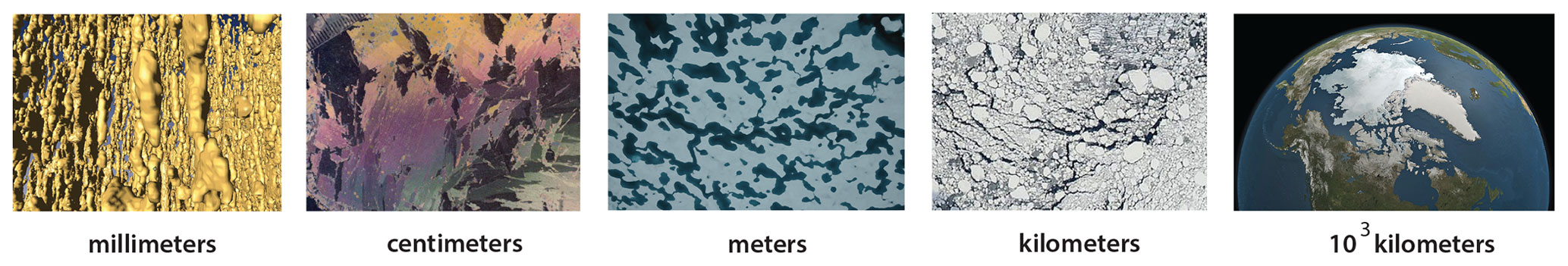
Figure 1Sea ice as a multiscale composite material. From left to right: millimeter-scale brine inclusions that form the porous microstructure of sea ice (Golden et al., 2007); centimeter-scale polycrystalline structure of sea ice (Arcone et al., 1986); melt ponds on Arctic sea ice in late spring and summer (Don Perovich) turning the surface into a two-phase composite of ice and melt water; the sea ice pack as a granular composite viewed from space (NASA), with “grains” ranging in horizontal extent from meters to tens of kilometers; and the Arctic Ocean viewed from space (NASA).
One of the fascinating, yet formidable aspects of modeling sea ice and its role in global climate is the sheer range of relevant length scales – over 10 orders of magnitude, from the sub-millimeter scale to thousands of kilometers, as indicated in Fig. 1. Modeling the macroscopic behavior of sea ice on scales appropriate for climate models and process studies depends on understanding the properties of sea ice on finer scales, down to individual floes and even the scale of the brine inclusions which control many of the distinct physical characteristics of sea ice as a material. Climate models challenge the most powerful supercomputers to their fullest capacity. However, even the largest computers still limit the resolution to tens of kilometers and typically require clever approximations and parameterizations to incorporate the basic physics of sea ice (Golden et al., 2020; Golden, 2015, 2009). One of the fundamental challenges in modeling sea ice – and a central theme in what follows – is how to account for the influence of the microscale on macroscopic behavior, that is, how to rigorously use information about smaller scales to predict effective behavior on larger scales. Here we consider three different homogenization problems in the physics of sea ice: the classic two-phase problem of brine inclusions in an ice host; sea ice as a polycrystalline material; and advection diffusion processes such as thermal conduction or nutrient diffusion in the presence of, e.g., convective brine flow. All of these questions are also of particular interest in polar microbial ecology (Thomas and Dieckmann, 2003; Reimer et al., 2022).
We observe that this central problem of finding the effective properties of sea ice is analogous to the main focus of statistical mechanics, where the dynamics of molecular interactions are used to find the macroscopic behavior of physical systems (Thompson, 1988; Christensen and Moloney, 2005). Moreover, mathematical homogenization theory for differential equations with random coefficients similarly seeks to find the large-scale effective behavior from some knowledge about the local coefficients (Milton, 2002; Torquato, 2002; Bensoussan et al., 1978; Papanicolaou and Varadhan, 1982; Kozlov, 1989). These fields of physics and applied mathematics provide a natural framework for treating sea ice in predictive models of climate and improving projections of how Earth's polar ice packs may evolve in the future.
The analytic continuation method (ACM) (Bergman, 1980; Milton, 1980; Golden and Papanicolaou, 1983; Golden, 1997b; Milton, 2002), in particular, yields powerful integral representations for the effective or homogenized transport coefficients of two-component (Golden and Papanicolaou, 1983) or multicomponent (Golden and Papanicolaou, 1985; Golden, 1986) media. The method exploits the properties of these coefficients as analytic functions of ratios of the constituent parameters for two-phase media, such as the ratio of the electrical or thermal conductivities or the complex permittivities. The geometry of the composite microstructure is encoded into a self-adjoint operator G through the characteristic function which takes the values 1 in one component (brine) and 0 in the other (ice). The key step in obtaining the integral representation, say in the case of electrical conductivity, is to derive a formula for the local electric field in terms of the resolvent of G and then apply the spectral theorem in an appropriate Hilbert space. This representation for the effective conductivity (or effective complex permittivity) achieves a complete separation between the component parameters in the variable and the geometry of the microstructure embedded in the spectral measure of G. In a discrete model of a composite, the operator G becomes a random matrix, whose eigenvalues and eigenvectors can be used to compute the spectral measure (Murphy et al., 2015).
The Stieltjes or Herglotz structure of the effective parameters and their integral representations can be used to find rigorous bounds on the homogenized transport coefficients (Bergman, 1980; Milton, 1980; Golden and Papanicolaou, 1983; Golden, 1986; Baker and Graves-Morris, 1996; Milton, 2002; Gully et al., 2015; Cherkaev, 2019). The bounds are based on knowledge of the moments of the spectral measure or the correlation functions of the composite microstructure. Bounds on the complex permittivity of sea ice as a two-phase composite were first obtained in the context of remote sensing and the mathematical analysis of sea ice electromagnetic properties (Golden, 1995; Golden et al., 1998b, c). For example, the mass of the spectral measure is the brine volume fraction. If this is known, then one can obtain elementary bounds in the complex case, which reduce to the classical arithmetic and harmonic mean bounds for real parameters. If the microgeometry is further assumed to be statistically isotropic, then tighter Hashin-Shtrikman bounds can be obtained. Tighter bounds can be obtained when the composite is assumed to have a matrix-particle structure, e.g., separated brine inclusions in a pure ice host (Bruno, 1991; Golden, 1997b). Such structure leads to gaps in the spectrum of G and tighter constraints on the support of the spectral measure.
In remote sensing applications of the inverse homogenization problem (Cherkaev and Golden, 1998; Cherkaev, 2001), one uses measurements of bulk electromagnetic behavior, such as the effective complex permittivity, to obtain information about the spectral measure (Cherkaev, 2001) and bounds on the microstructural characteristics, such as the brine volume fraction, connectivity (Cherkaev and Tripp, 1996; Cherkaev and Golden, 1998; Golden et al., 1998b; Gully et al., 2007; Orum et al., 2012; Cherkaev and Bonifasi-Lista, 2011), and crystal orientation (Gully et al., 2015). The microscale structure, which determines the spectral measure and the homogenized coefficient, is thus linked to the macroscopic behavior via the operator G and its spectral characteristics, and vice versa. In the multicomponent case with three or more constituents, the homogenized transport coefficients are analytic functions of two or more complex variables, and a polydisc representation formula was found to obtain rigorous bounds (Golden and Papanicolaou, 1985; Golden, 1986).
The first area of application where the ACM was extended beyond the classical case of two-component and multiphase composites is diffusive transport in the presence of a flow field, which is widely encountered throughout science and engineering (McLaughlin et al., 1985; Biferale et al., 1995; Fannjiang and Papanicolaou, 1994, 1997; Pavliotis, 2002; Majda and Kramer, 1999; Majda and Souganidis, 1994; Xin, 2009). In addition to thermal, saline, and nutrient transport through the porous microstructure of sea ice, large-scale transport of ice floes and heat are also advection diffusion processes. Avellaneda and Majda (1989, 1991) found a Stieltjes integral representation for the effective diffusivity as a function of the Péclet number for diffusion in an incompressible velocity field. Based on the approach in Golden and Papanicolaou (1983), they set up a Hilbert space framework and applied the spectral theorem to a resolvent representation involving analogues of G and the electric field, where the spectral measure depends on the geometry of the velocity field, and knowledge of its moments yields bounds on the effective diffusivity. In Murphy et al. (2017b, 2020a) we proved novel versions of the Stieltjes formulas. We also developed a framework to numerically compute the spectral measures and a systematic method to find its moments – and thus a hierarchy of bounds (Bergman, 1982; Golden, 1986) for both the time-dependent and time-independent cases.
In another extension of the ACM to a large class of media, a Stieltjes integral representation and rigorous bounds for the effective complex permittivity of polycrystalline media were developed in Gully et al. (2015), based on a resolvent formula for the electric field and earlier observations in Milton (1981), Bergman and Stroud (1992), and Milton (2002). The bounds assume knowledge of the average crystal orientation and the complex permittivity tensor of an individual crystal grain. In sea ice, finding the complex permittivity tensor of an individual crystal involves homogenizing the smaller-scale brine microstructure (Gully et al., 2015). The polycrystalline structure of sea ice, as characterized by the statistics of grain size, shape, and orientation, is influenced by the conditions under which the ice was grown (Weeks and Ackley, 1982; Petrich and Eicken, 2009; Untersteiner, 1986). For example, while sea ice grown in quiescent conditions tends to have rather large-grained columnar structure, when grown in more turbulent or wavy conditions, it typically has a fine-grained granular structure. These distinctly different ice types have quite different fluid flow properties (Golden et al., 1998a). Additionally, when there is a well-defined current direction during formation, crystal orientations tend to be statistically anisotropic within the horizontal plane (Weeks and Gow, 1980). This can significantly affect the sea ice radar signature used in measurements of sea ice thickness and other properties used to validate climate models (Golden and Ackley, 1981).
The interaction of ocean surface waves with polar sea ice is a critical process in Earth's climate system; its accurate representation is of great importance for developing efficient climate models. Declining summer sea ice has increased wave activity and the importance of ice–ocean interactions in the Arctic (Waseda et al., 2018). The Arctic marginal ice zone (MIZ), the transitional region between dense pack ice and open ocean characterized by strong wave-ice and atmosphere–ice–ocean interactions, has widened significantly (Strong and Rigor, 2013). These recent changes can have complex implications for both sea ice formation and melting (Li et al., 2021). Indeed, the propagation of surface waves through Earth's sea ice covers is a complex phenomenon that drives their growth and decay. One of the main approaches to studying waves in sea ice which is valid when wavelengths are much greater than floe sizes is to model the surface layer of the ice-covered ocean as a continuum with effective properties (Bates and Shapiro, 1980; Keller, 1998; Wang and Shen, 2010; Mosig et al., 2015). Recently, this fundamental problem in sea ice physics was homogenized with a Stieltjes integral representation for the effective complex viscoelasticity of the surface layer, based on a resolvent formula for the local strain field (Sampson, 2017). The integral involves a spectral measure of a self-adjoint operator which depends on the geometry of the floe configurations. The mass of the spectral measure is the area fraction of the ocean covered by sea ice, which is a standard satellite data product known as the sea ice concentration field. If the measure's mass is known, rigorous bounds can be obtained on the complex viscoelastic parameter. Previously, this effective parameter had only been fitted to wave data.
Early on in our work in extending the ACM to the above problems in sea ice physics, it was clear that the classical approach based on bounding effective parameters using the moments of the spectral measure would, in many cases, have limited effectiveness. Bounds with only a moment or two known can be quite wide, particularly for a high contrast in the properties of the constituents, like in sea ice. We then developed a framework in the classic two-phase case for computing the spectral measure through discretization of the relevant microstructures and finding the eigenvalues and eigenvectors of the matrix representation of G. By developing the mathematical foundation for these computations (Murphy et al., 2015) and studying the properties of computed spectral measures for a broad range of sea ice and other microstructures, like human bone (Golden et al., 2011; Bonifasi-Lista and Cherkaev, 2008, 2009; Bonifasi-Lista et al., 2009; Cherkaev and Bonifasi-Lista, 2011), we discovered that eigenvalue statistics displayed fascinating behavior depending on the connectedness of one of the phases.
The statistical behavior of the spectrum is related to the extent that the eigenfunctions overlap. A key example is the Anderson theory of the metal–insulator transition (MIT) (Anderson, 1958; Evers and Mirlin, 2008), which provides a powerful theoretical framework for understanding when a disordered medium allows electronic transport and when it does not. Indeed, for large enough disorder, the electrons are localized in different places with uncorrelated energy levels described by Poisson statistics (Shklovskii et al., 1993; Kravtsov and Muttalib, 1997). For small disorder, the wave functions are extended and overlap, giving rise to correlated Wigner–Dyson (WD) statistics (Shklovskii et al., 1993; Kravtsov and Muttalib, 1997) with strong level repulsion (Guhr et al., 1998). In work on the effective complex permittivity for electromagnetic wave propagation through two-phase composites in the long wavelength regime (or other transport coefficients such as thermal or electrical conductivity), we found an Anderson transition in spectral characteristics as the microstructure developed long-range order in the approach to a percolation threshold (Murphy et al., 2017a). We observed transitions in localization characteristics of the field vectors and associated transitions in spectral behavior from uncorrelated Poissonian statistics to universal (repulsive) Wigner–Dyson statistics, reminiscent of the Gaussian orthogonal ensemble (GOE) in random matrix theory. Moreover, mobility edges appear in a manner akin to Anderson localization, where such edges mark the characteristic energies of the quantum MIT (Guhr et al., 1998). In Morison et al. (2022) a novel class of two-phase media was introduced – twisted bilayer composites – based on Moiré patterns, that display exotic effective properties and dramatic transitions in spectral behavior with very small changes in system parameters.
We have laid the groundwork for rigorous mathematical modeling of sea ice processes using Stieltjes integral representations for homogenized parameters in several contexts of importance (Murphy and Golden, 2012; Murphy et al., 2015; Gully et al., 2015; Murphy et al., 2017a, b, 2020a; Golden et al., 2020; Golden, 2015, 2009, 1997b; Golden et al., 1998b, c). We also mention a significant recent advance in obtaining a Stieltjes integral representation for the fluid permeability of a porous medium (Bi et al., 2023) and an excellent, recent review of Stieltjes integrals in materials science (Luger and Ou, 2022; Ou and Luger, 2022). The permeability result is relevant for sea ice modeling (Golden et al., 1998a, 2007; Golden, 2009) and has eluded mathematical inquiry for quite some time.
We have focused here on the central role that the composite “microgeometry” plays – via the operator G and its spectral measure (and analogues) – in determining effective behavior on scales relevant to coarse-grained climate models and studies of sea ice processes. The geometry represents different composite structures in different contexts. At the finest scales, the millimeter-scale brine inclusion microstructure determines the properties of individual sea ice crystallites, whose size and orientation statistics make up the centimeter-scale polycrystalline microgeometry. Convective fluid flow fields help transport heat, salt, and nutrients, where the flow field geometry on centimeter to meter scales plays the role of the composite microstructure in advection–diffusion processes. Ponds on the surface of melting Arctic sea ice floes define the microgeometry of the surface composite of melt water and snow on meter to kilometer scales. The surface layer of the ocean is a composite of sea water and sea ice, with microgeometry defined by the concentration, geometry, and arrangement of the ice floes on scales of meters to tens of kilometers. Large-scale ice pack dynamics and transport on the scale of the Arctic Ocean are determined primarily by advective and thermal forcing. The “microstructure” of these advective wind and current fields, as well as the temperature field, can be on scales from meters to hundreds of kilometers.
Stieltjes integral representations provide information on a wide range of transport parameters, including electrical and thermal conductivity, complex permittivity, diffusion coefficient, and fluid permeability. These parameters can be used as direct inputs into physical, biogeochemical, and ecological models of sea ice processes and in large-scale numerical models. The interplay between homogenization techniques like the analytic continuation method here and models of phase transitions in statistical physics (Banwell et al., 2023) is particularly interesting across the full range of scales. From the millimeter-scale brine inclusions (Golden et al., 1998a, 2007) to meter-scale melt ponds (Ma et al., 2019) and the thermal properties of the ice pack itself, our Stieltjes representations provide rigorous theories of how effective parameters depend on the constituent parameters and mixture geometries. Finally, we note that in applications of the ACM to wave phenomena, such as the effective complex permittivity for electromagnetic waves propagating through the sea ice, the theory holds in the quasistatic regime where the wavelength in the medium is assumed to be much longer than the microstructural scale. Typically, electromagnetic waves in the megahertz and low gigahertz frequency ranges satisfy this condition. For the effective complex viscoelasticity of the upper layer of the ocean, the Stieltjes representation holds again in the quasistatic regime where the wavelength is larger than the typical floe size.
The analytic continuation method is a powerful approach in homogenization that provides a robust mathematical framework for rigorously studying effective properties in the sea ice system. The body of work that is discussed here will advance our sea ice modeling capabilities and how sea ice is represented in global climate models, which will improve projections of the fate of sea ice and the ecosystems it supports. Moreover, the functions we study here in the sea ice context share the same mathematical properties as effective parameters in many other areas of science and engineering. Indeed, our work based on Stieltjes integrals has advanced the physics of materials related to twisted bilayer graphene and quasicrystals (Morison et al., 2022), biomedical engineering of human bone (Golden et al., 2011; Bonifasi-Lista and Cherkaev, 2008, 2009; Bonifasi-Lista et al., 2009; Cherkaev and Bonifasi-Lista, 2011), and our understanding of the physical properties of general polycrystalline media in geosciences and other fields (Gully et al., 2015; Cherkaev, 2019).
Connectedness of one phase in a composite material is often the principal feature of the mixture geometry which determines effective behavior. For example, if highly conducting inclusions are sparsely distributed, forming a disconnected phase within a poorly conducting encompassing host, then the effective conductivity will be poor as well. However, if there are enough conducting inclusions so that they form connected pathways through the medium, then the effective conductivity will be much closer to that of the inclusions. Percolation theory (Broadbent and Hammersley, 1957; Stauffer and Aharony, 1992; Grimmett, 1989; Bunde and Havlin, 1991) focuses on connectedness in disordered and inhomogeneous media and has provided the theoretical framework for describing the behavior of fluid flow through sea ice (Golden et al., 1998a, 2007; Golden, 2009).
Consider the d-dimensional integer lattice ℤd, and the square or cubic network of bonds joining nearest-neighbor lattice sites. In the percolation model (Broadbent and Hammersley, 1957; Stauffer and Aharony, 1992; Grimmett, 1989; Bunde and Havlin, 1991), we assign to each bond a conductivity σ0>0 with probability p, meaning it is open (black), and with probability 1−p we assign σ0=0, meaning it is closed. Two examples of lattice configurations are shown in Fig. 2 with in (a) and in (b). Groups of connected open bonds are called open clusters. In this model there is a critical probability pc, , the percolation threshold, at which the average cluster size diverges and an infinite cluster appears. For the d=2 bond lattice, . For p<pc the infinite cluster density P∞(p)=0, while for p>pc, P∞(p)>0 and near the threshold, as , where β is a universal critical exponent. It depends only on dimension and not on the details of the lattice. Let and τ(x,y) be the probability that x and y belong to the same open cluster. Then for p<pc, , and the correlation length diverges with a universal critical exponent ν as , as shown in Fig. 2c.
The effective conductivity σ*(p) of the lattice, now viewed as a random resistor (or conductor) network, defined via Kirchoff's laws, vanishes for p<pc like P∞(p) since there are no infinite pathways, as shown in Fig. 2e. For p>pc, , and near pc, where t is the conductivity critical exponent, with in (Golden, 1990, 1992, 1997a), and numerical values t≈1.3 in d=2 and t≈2.0 in d=3 (Stauffer and Aharony, 1992). Consider a random pipe network with fluid permeability k*(p) exhibiting similar behavior where e is the permeability critical exponent, with e=t (Chayes and Chayes, 1986; Sahimi, 1995; Golden, 1997a). Both t and e are believed to be universal – they depend only on dimension and not the lattice. Continuum models such as the Swiss cheese model can exhibit nonuniversal behavior with exponents different from the lattice case and e≠t (Halperin et al., 1985; Feng et al., 1987; Stauffer and Aharony, 1992; Sahimi, 1994; Kerstein, 1983).
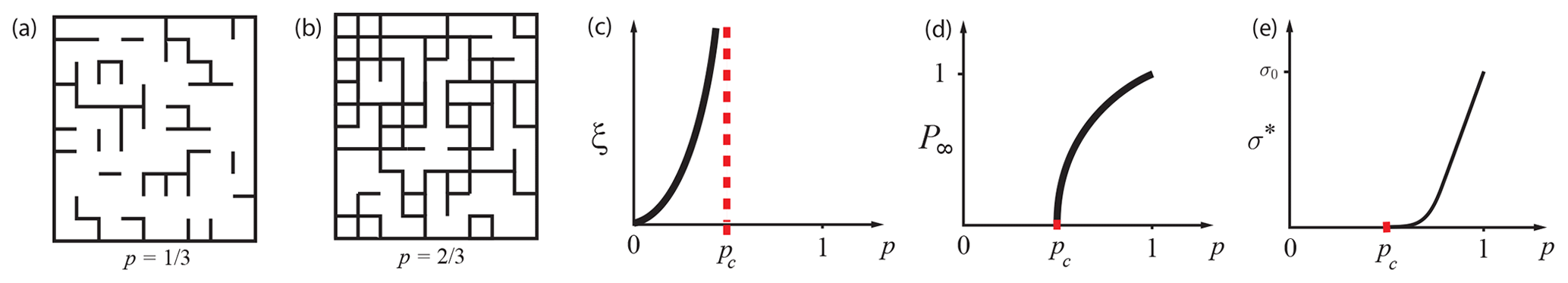
Figure 2The two-dimensional square lattice percolation model below its percolation threshold of in (a) and above it in (b). (c) Divergence of the correlation length as p approaches pc. The infinite cluster density of the percolation model is shown in (d), and the effective conductivity is shown in (e).
We now describe the analytic continuation method (ACM) for studying the effective properties of composites (Bergman, 1980; Milton, 1980; Golden and Papanicolaou, 1983; Golden, 1997b). This method has been used to obtain rigorous bounds on bulk transport coefficients of composite materials from partial knowledge of the microstructure, such as the volume fractions of the phases. Examples of transport coefficients to which this approach applies include the complex permittivity, electrical and thermal conductivity, diffusivity, magnetic permeability, and elasticity (Cherkaev, 2001; Cherkaev and Bonifasi-Lista, 2011; Cherkaev, 2019; Ou and Cherkaev, 2006; Ou, 2012; Kantor and Bergman, 1982; Avellaneda and Majda, 1989, 1991; Murphy et al., 2020b, 2017b). In the works of Golden (Golden, 1995, 1997b, 2015, 2009; Golden et al., 1998b, c, 2020), rigorous bounds on the complex permittivity of sea ice were found.
To set ideas we focus on the complex permittivity, keeping in mind the broad applicability of the ACM. Consider a two-phase random medium with local permittivity tensor ϵ(x,ω), a spatially stationary random field in x∈ℝd and ω∈Ω, where Ω is the set of realizations of the medium. We consider a two-phase locally isotropic medium, where the components ϵjk, , of ϵ satisfy
where d is dimension, δjk is the Kronecker delta, and
Later, we will consider a polycrystalline medium where ϵ is a non-trivial symmetric matrix. Here, χi(x,ω) is the characteristic function of medium , equaling 1 for ω∈Ω with medium i at x and 0 otherwise, with . The random electric and displacement fields E(x,ω) and D(x,ω) satisfy
A variational problem (Golden and Papanicolaou, 1983) establishes that E can be written as satisfying
In simpler terms, this says that curl-free and divergence-free fields are orthogonal (Helmholtz's theorem).
The effective permittivity tensor ϵ* is defined as , where 〈⋅〉 is ensemble averaging over Ω or, by an ergodic theorem, spatial average over all of ℝd (Golden and Papanicolaou, 1983). We prescribe that E0 has direction ek, the kth direction unit vector, and focus on the diagonal coefficient , with . The key step of the method is to obtain the following Stieltjes integral representation for ϵ* (Bergman, 1978; Milton, 1980; Golden and Papanicolaou, 1983; Milton, 2002):
where μ is a positive Stieltjes measure with support in [0,1], and F plays the role of a (negative) electric susceptibility (Bergman, 1978). In the variable , with , F(s) is a Stieltjes function (Golden, 1997c; Cherkaev, 2001; Murphy and Golden, 2012). This representation arises from a resolvent formula for the electric field (in medium 1) (Murphy et al., 2015; Cherkaev, 2001; Golden and Papanicolaou, 1983):
yielding , where is a projection onto the range of the gradient operator ∇ and I is the identity operator. Equation (5) is the spectral representation of the resolvent formula in Eq. (6), and μ is a spectral measure of the self-adjoint operator G=χ1Γχ1 on L2(Ω,P).
A critical feature of Eq. (5) is that the component parameters in s are separated from the geometrical information in μ. Information about the geometry enters through the moments
Then μ0=ϕ, where ϕ is the volume or area fraction of phase 1, such as the brine volume fraction, the open-water area fraction, or melt pond coverage, and if the material is statistically isotropic. In general, μn depends on the (n+1)-point correlation function of the medium. This integral representation yields rigorous forward bounds for the effective parameters of composites, given partial information on the microgeometry via the μn (Bergman, 1980; Milton, 1980; Golden and Papanicolaou, 1983; Bergman, 1982). The integral representations can also yield inverse bounds, allowing one to use data about the electromagnetic response of a sample to bound its structural parameters such as the volume fraction of each of the components (McPhedran et al., 1982; McPhedran and Milton, 1990; Cherkaev and Tripp, 1996; Cherkaev and Golden, 1998; Cherkaev, 2001; Zhang and Cherkaev, 2009; Bonifasi-Lista and Cherkaev, 2009; Cherkaev and Bonifasi-Lista, 2011; Day and Thorpe, 1999; Golden et al., 2011; Cherkaev, 2020). See Sect. 5 for more details.
3.1 Spectral measure computations for two-phase composites
Computing the spectral measure μ for a given 2D composite microstructure first involves discretizing a two-phase image of the composite into a square lattice filled with 1s and 0s corresponding to the two phases. On this square lattice, the action of the differential operators ∇ and ∇⋅ is defined in terms of forward- and backward-difference operators (Golden, 1992; Murphy et al., 2015). Then the key operator χ1Γχ1, which depends on the geometry of the network via χ1, becomes a real-symmetric matrix M (Murphy et al., 2015). Here Γ is a (non-random) projection matrix which depends only on the lattice topology and boundary conditions, and χ1 is a diagonal (random) projection matrix which determines the geometry and component connectivity of the composite medium (Gully et al., 2015; Murphy et al., 2015). Another spectral approach to finding effective properties based on analytic continuation relies on computation of the electromagnetic eigenstates of individual inclusions (Bergman et al., 2020; Bergman, 2022).
The powerful integral representation in Eq. (5) is formulated in a continuum setting. However, in order to actually compute the spectral measures, we must discretize, for example, an image of the brine inclusions or ice floes onto a lattice, and represent the operator G as a matrix. The following theorem provides a rigorous mathematical formulation of integral representations for the effective parameters for finite-lattice approximations of two-component media and tells how to compute the spectral measures. The electric field decomposition in this theorem is established using the fundamental theorem of linear algebra and orthogonality properties of the ranges and kernels of matrix representations for ∇, ∇×, and ∇⋅ (Huang et al., 2019) and will be published elsewhere. The integral representation in Eq. (8) is established in Theorem 2.1 of Murphy et al. (2015).
For each ω∈Ω, let M(ω)=W(ω)Λ(ω) WT(ω) be the eigenvalue decomposition of the real-symmetric matrix M(ω)=χ1(ω) Γ χ1(ω). Here, the columns of the matrix W(ω) consist of the orthonormal eigenvectors wi(ω), , of M(ω), and the diagonal matrix involves its eigenvalues λi(ω). Denote the projection matrix onto the eigenspace spanned by wi and denote the Dirac δ measure centered at λi. The electric field E(ω) satisfies , with E0=〈E(ω)〉 and ΓE(ω)=Ef(ω), and χ1E satisfies the resolvent formula in Eq. (6) with G replaced by M. The effective complex permittivity tensor ϵ* has components , , which satisfy
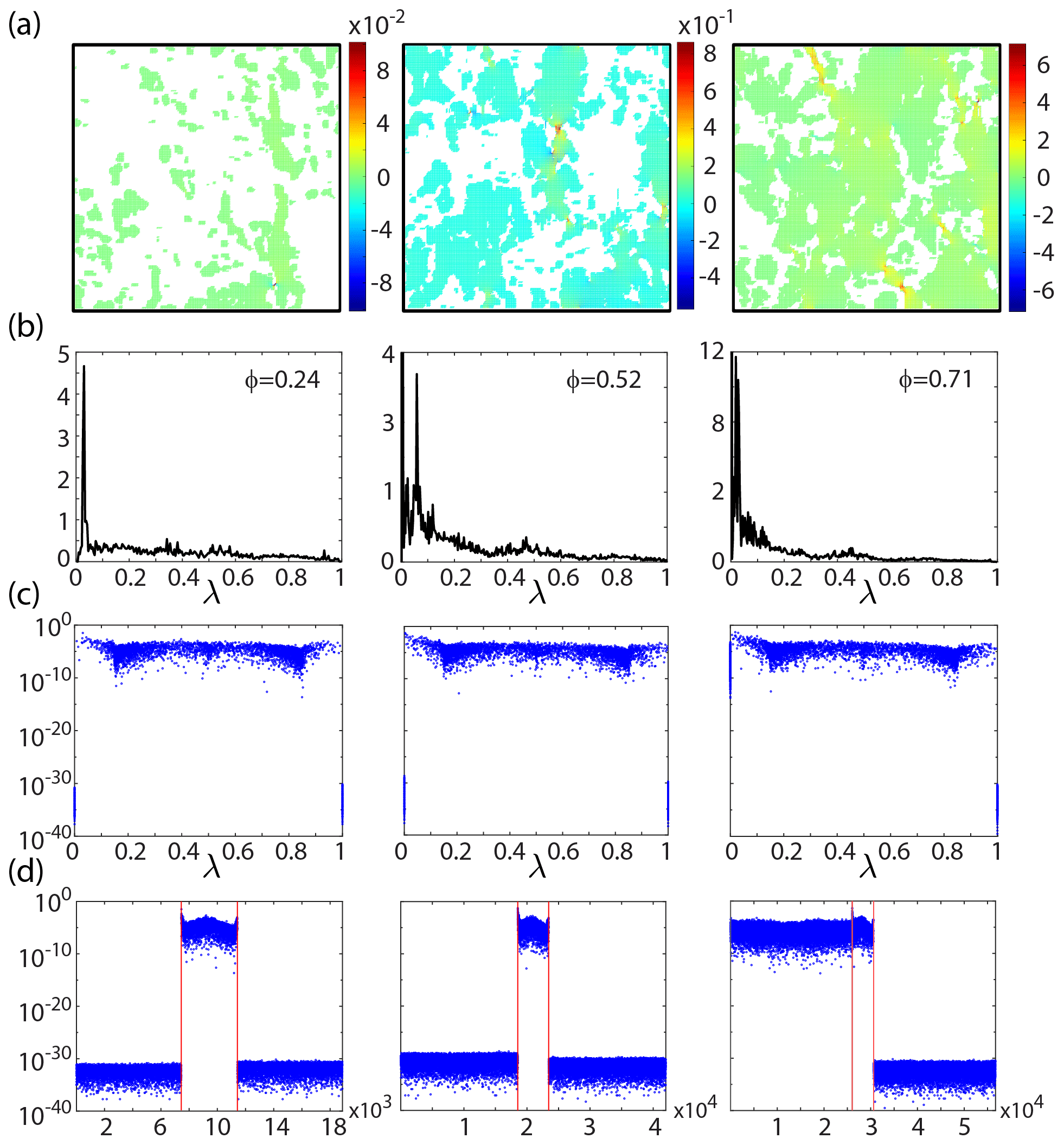
Figure 3Electric fields and spectral measures for sea ice brine microstructure. (a) Electric field values in log-10 scale for X-ray CT images of 2D vertical cross sections of sea ice brine microstructure, with increasing connectivity from left to right. (b) Corresponding spectral functions μ(λ) (histogram representations) of the spectral measure μ in (c) and (d), which display spectral weights versus the associated eigenvalues λi of the matrix M and index i, respectively, where ϕ is the brine area fraction of the images in (a). The vertical bars in (d) delineate the δ functions at the spectral endpoints seen in (c) from the rest of the spectrum, where and . As the percentage of brine increases, the fluid phase becomes increasingly connected, resulting in a substantial increase in the strength of the electric field, with “hot spots” forming in geometric bottlenecks. Macroscopic connectivity of the brine phase is characterized by the mass of the δ function at λ=0 switching from numerically zero, with the , to , giving rise to the “hot spots” in E via Eq. (9). The electrical permittivity is taken to be for brine and ε2=3.06 for ice (Backstrom and Eicken, 2006). E0 is taken to be vertically oriented.
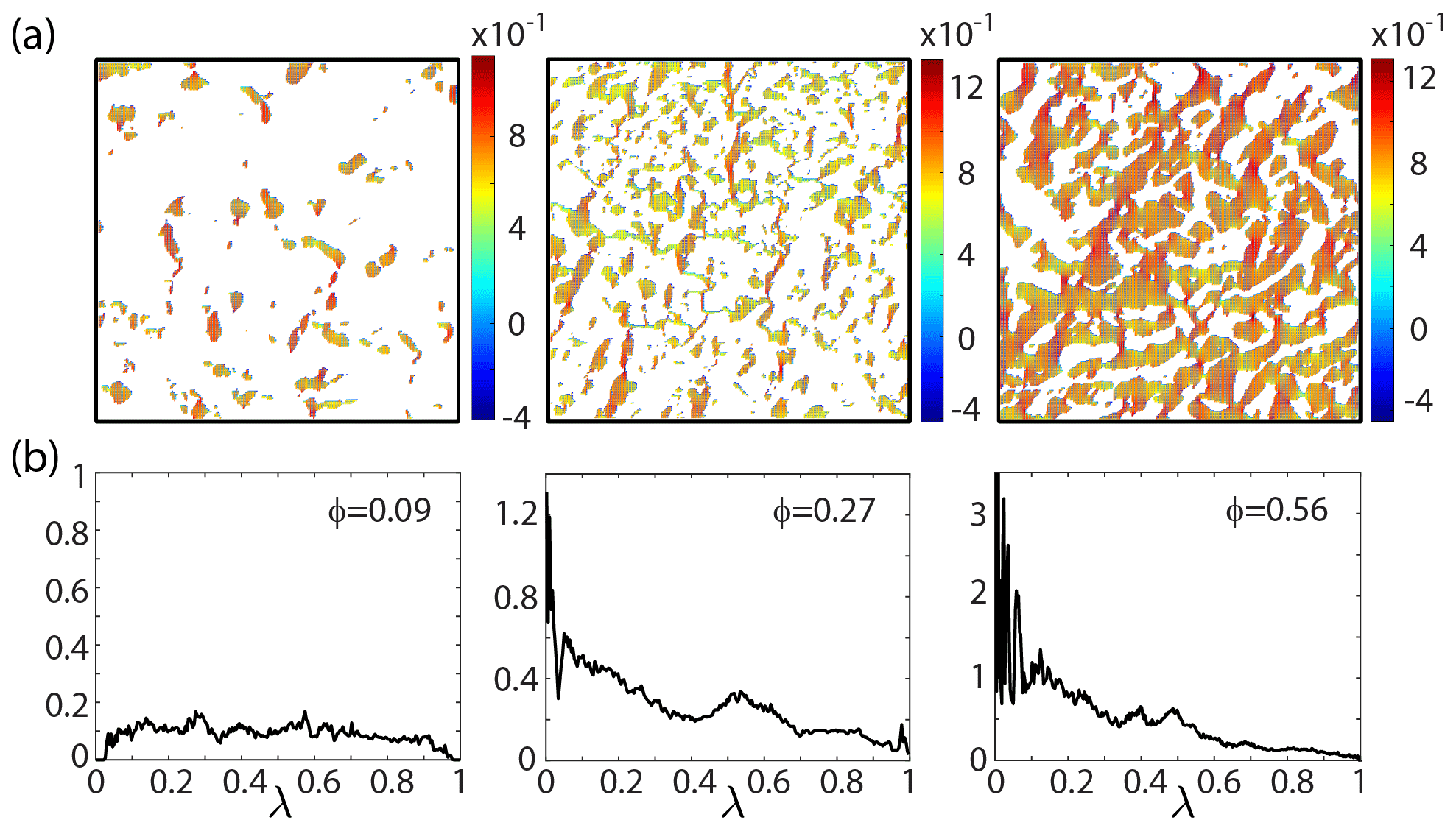
Figure 4Temperature gradient fields and spectral functions for sea ice melt pond microstructure. (a) Temperature gradient field values in log-10 scale for melt pond microstructure atop Arctic sea ice, with increasing connectivity from left to right (images courtesy of Don Perovich), with corresponding spectral functions μ(λ) displayed below in (b). Here the gradient of temperature T, −∇T, plays the role of Ef in Eqs. (3) and (4) (Milton, 2002) ( for some electrical potential φ); the component thermal conductivities κi, , play the role of the complex electrical permittivities ϵi; and the heat current Q plays the role of the displacement field D; here, ϕ is the melt pond area fraction for the images in (a). Analogous to Fig. 3, as the fluid phase becomes increasingly connected on macroscopic length scales, a buildup of spectral measure mass at λ=0 shown in (b) leads to the formation of a δ function at λ=0, with corresponding switching in the values of the from numerically zero, with the for the left an middle figure panels, to for the rightmost panel. The δ function at λ=1 is also analogous to that in Fig. 3. Like E0 in Fig. 3, we take the average thermal gradient to be vertically oriented. The thermal conductivity is taken to be κ1=0.5606 W m−1 K−1 for melt ponds and κ2=0.3073 W m−1 K−1 for the surrounding snow (Yen, 1981).
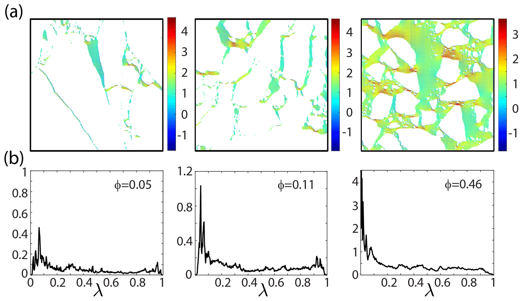
Figure 5Temperature gradient fields and spectral functions for Arctic pack ice microstructure. (a) Temperature gradient field values in log-10 scale for Arctic pack ice microstructure, with increasing connectivity from left to right (images courtesy of Don Perovich), with corresponding spectral functions μ(λ) displayed below in (b). Analogous to Fig. 3, as the fluid phase becomes increasingly connected on macroscopic length scales, a buildup of spectral measure mass at λ=0 shown in (b) leads to the formation of a δ function at λ=0; here, ϕ is the open-ocean area fraction for the images in (a). We see a corresponding switching in the values of the from numerically zero, with the for the left and middle figure panels, to for the rightmost panel. The δ function at λ=1 is also analogous to that in Fig. 3. Like E0 in Fig. 3, we take the average thermal gradient to be vertically oriented. Thermal conductivity is taken to be κ1=0.57 W m−1 K−1 for ocean and κ2=2.11 W m−1 K−1 for ice floes (Pringle et al., 2006).
From Theorem 1, the integral and χ1E in Eqs. (5) and (6) have explicit representations in terms of the eigenvalues λi and eigenvectors wi of M (Murphy et al., 2015, 2017a),
where plays the role of a standard basis vector on the lattice. To compute μ, a non-standard generalization of the spectral theorem for matrices is required, due to the projective nature of the matrices χ1 and Γ (Murphy et al., 2015). We developed a projection method that shows the spectral measure μ in Eq. (8) depends only on the eigenvalues and eigenvectors of random submatrices of Γ of size N1≈ϕN. They correspond to diagonal components [χ1]ii=1, as the spectral weights mi (Christoffel numbers) associated with eigenvectors satisfying χ1wi=0 are themselves zero, mi=0 (Murphy et al., 2015). Fortunately, since these submatrices are much smaller for low volume fractions, this method greatly improves the efficiency and accuracy of numerical computations of μ.
The measure μ exhibits fascinating transitional behavior as a function of system connectivity. For example, in the case of a random resistor network (RRN) with a low volume fraction p of open bonds, as shown in Fig. 2a, there are spectrum-free regions at the spectral endpoints (Murphy and Golden, 2012; Murphy et al., 2015). However, as p approaches the percolation threshold pc (Stauffer and Aharony, 1992; Torquato, 2002) and the system becomes increasingly connected, these spectral gaps shrink and then vanish (Murphy and Golden, 2012; Jonckheere and Luck, 1998), leading to the formation of δ components of μ at the spectral endpoints, precisely (Murphy and Golden, 2012) when p=pc (and in d=3). This leads to critical behavior of σ* for insulating/conducting and conducting/superconducting systems (Murphy and Golden, 2012). This gap behavior of μ has led (Golden, 1997c; Murphy and Golden, 2012) to a detailed description of these critical transitions in which is analogous to the Lee–Yang–Ruelle–Baker description (Baker, 1990; Golden, 1997c) of the Ising model phase transition in the magnetization M. Moreover, using this gap behavior, all of the classical critical exponent scaling relations were recovered (Murphy and Golden, 2012; Golden, 1997c) without heuristic scaling forms (Efros and Shklovskii, 1976) but instead by using the rigorous integral representation for σ* involving μ.
This spectral behavior emerges in all the systems mentioned above, such as the brine microstructure of sea ice (Golden et al., 1998a, 2007; Golden, 2009) as shown in Fig. 3, melt ponds on the surface of Arctic sea ice (Hohenegger et al., 2012) as shown in Fig. 4, and the sea ice pack itself (Murphy et al., 2017a) in Fig. 5. This also gives rise to critical behavior of the electric field, as shown in Fig. 3 for 2D cross sections of 3D brine microstructure, with E0 taken to be in the vertical direction. Disconnected and weakly connected examples of brine microstructure have small values of the electric field, while strongly connected brine microstructures are characterized by a substantial increase in the electric field's strength, with “hot spots” forming in geometric bottlenecks. A similar behavior is exhibited by the temperature gradient ∇T associated with the Stieltjes integral for the effective thermal conductivity κ*, as shown for melt ponds atop Arctic sea ice in Fig. 4 and for Arctic pack ice in Fig. 5.
3.2 Generalization to rank deficient setting
In the periodic setting, for example, the matrix Laplacian is singular, so the matrix representation of in Γ is not defined. We now extend the mathematical framework developed in Murphy et al. (2015) to this setting. To make the connection to the abstract Hilbert space (Golden and Papanicolaou, 1983) and full-rank matrix (Murphy et al., 2015) settings, we first give relevant details for these cases. Equation (6) for the abstract Hilbert space setting follows by applying the operator to the formula , yielding ΓD=0. Equation (6) then follows by using ΓEf=Ef and ΓE0=0 (Murphy et al., 2015), since Ef is in the range of Γ and E0 is constant (Murphy et al., 2020a, 2017b, 2015). The matrix form of is , where ∇ now represents the finite-difference matrix representation of the gradient operator and −∇T is the finite-difference representation of the divergence operator, with negative matrix Laplacian given by ∇T∇ (Murphy et al., 2015). As before, in Murphy et al. (2015) we applied the matrix ∇(∇T∇)−1 to the formula , yielding ΓD=0, where , and Eq. (6) follows the same way as before, using the fact that E0 is in the orthogonal complement of the range of ∇, so ΓE0=0.
Now consider the singular value decomposition of the matrix gradient (Murphy et al., 2020a) of size m×n, say, ∇=UΣVT. Here U is a m×n matrix satisfying UTU=In; Σ is a n×n diagonal matrix with diagonal entries consisting of the singular values of ∇; and V is a n×n orthogonal matrix satisfying , where In is the identity matrix of size n. When the matrix gradient is full rank it has n strictly positive singular values, so Σ is an invertible matrix, and the matrix representation of Γ is given by Γ=UUT. On the other hand, when the matrix gradient is singular we have , where the diagonal matrix Σ1 contains the n1 strictly positive singular values of Σ and the rest of the singular values have value 0. Denoting U1 and V1 to be the columns of U and V corresponding to the diagonal entries of Σ1, we have , where Σ1 is invertible and . This enables us to write as ; hence and . Noting that the columns of U1 span the range of the matrix gradient ∇, the matrix is a projection onto the range of ∇ (Murphy et al., 2020a). Defining , Eq. (6) follows the same way as before, using the fact that E0 is in the orthogonal complement of the range of ∇ so ΓE0=0. This clearly generalizes the full-rank setting. More details will be published elsewhere.
Sea ice is a composite material with polycrystalline microstructure on the millimeter to centimeter scale. When sea water freezes under turbulent conditions, granular sea ice forms, which has small crystals with isotropic orientation angles. Columnar sea ice forms in quiescent conditions, with large crystals more strongly oriented in the vertical direction. Examples of granular and columnar sea ice polycrystalline microgeometries are displayed in Fig. 6a.
Our analysis of the transport properties of random, uniaxial polycrystalline media (Barabash and Stroud, 1999) in Gully et al. (2015), and a somewhat new formulation presented below, shows that the underlying mathematical framework is a direct analogue of that for two-phase random media discussed in Sect. 3. For simplicity, we discuss electrical permittivity ϵ, keeping in mind the broader applicability to thermal conductivity κ and electric conductivity σ, as well as viscoelastic modulus (Cherkaev, 2019), etc. Polycrystalline materials are composed of many crystallites (single crystals of varying size, shape, and orientation) that can have different local conductivities along different crystal axes. In contrast to Eq. (1), the local permittivity matrix of such media is given by (Milton, 2002; Barabash and Stroud, 1999):
where R(x,ω) is a random rotation matrix satisfying . For example, for d=2 we have
where is the orientation angle, measured from the direction e1 of the crystallite, which has an interior containing x∈ℝd for ω∈Ω. In higher dimensions, d≥3, the rotation matrix R is a composition of “basic” rotation matrices Rj, e.g., , where the matrix Rj(x,ω) rotates vectors in ℝd by an angle about the ej axis. For example, in three dimensions
In the case of uniaxial polycrystalline media, the local permittivity along one of the crystal axes has the value ϵ1, while the permittivity along all the other crystal axes has the value ϵ2, so for 2D (which is the general setting for 2D) and for 3D. Equation (10) can be written in a more suggestive form in terms of the matrix :
which is an analogue of Eq. (2). Here X1=RTCR and , where I is the identity matrix on ℝd. Since and C is a diagonal projection matrix satisfying C2=C, it is clear that the Xi, , are mutually orthogonal projection matrices satisfying
which are also properties of the characteristic functions χj in Sect. 3.
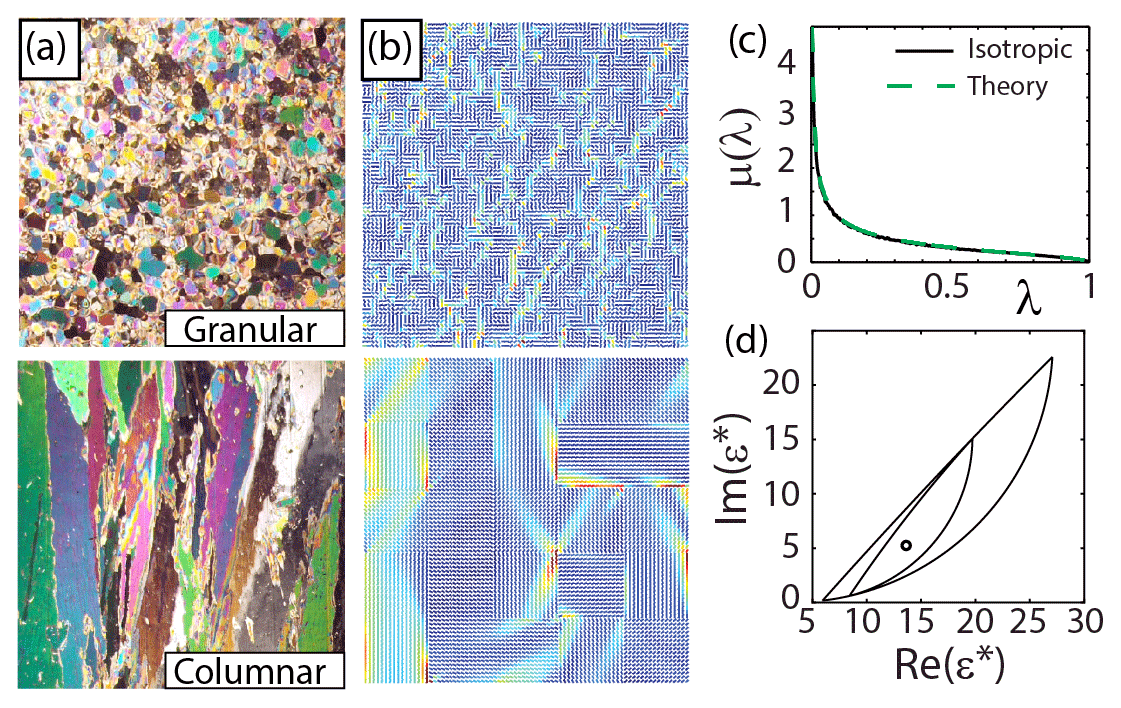
Figure 6Spectral analysis of polycrystalline media. (a) Cross sections of polycrystalline microstructure for granular and columnar sea ice (Jean-Louis Tyson). (b) Discrete checkerboard polycrystal microstructure with isotropic crystallite orientations within the horizontal plane, with small (top) and large (bottom) crystallite size. Cool and warm colors correspond to low- and high-displacement field values. (c) The spectral function, a histogram representation of the spectral measure μ(λ), shown along with its theoretical prediction for such isotropic media (Milton, 2002). (d) An example value of the complex effective permittivity of isotropic polycrystalline media captured by first- and second-order bounds (Gully et al., 2015).
Equations (3) and (4) are also satisfied in this polycrystalline setting (Golden and Papanicolaou, 1983). Similar to the derivation of Eq. (6) in Sect. 3, a resolvent representation for X1E follows by applying the operator to the formula , yielding ΓD=0. Then, using ΓEf=Ef and ΓE0=0 (Murphy et al., 2015) yields the following analogue of Eq. (6):
yielding the integral representation in Eq. (5) for . As in the two-component setting, a critical feature of Eq. (5) is that the component parameters in s are separated from the geometrical information in μ. Information about the geometry enters through the moments in Eq. (7), with G given in Eq. (15) and χ1 replaced by X1. The mass of the measure μjk is given by
where the second equality follows from the fact that X1 is a real-symmetric projection matrix. The statistical average in Eq. (16) can be thought of as the “mean orientation” or as the percentage of crystallites oriented in the kth direction. For example, in the case of two-dimensional polycrystalline media, d=2, Eq. (11) implies that
Generalizing Eq. (12), with , to dimensions d≥3 shows that is a linear combination of averages of the form , where .
Given partial information on the microgeometry incorporated into the moments μn, the integral representation (5) for this polycrystalline setting yields rigorous forward bounds for the effective parameters of composites (Gully et al., 2015; Milton, 2002), as shown in Fig. 6d. The integral representation can also be used to obtain inverse bounds that give estimates for the structural parameters of a composite derived from the electromagnetic response of a sample. One such structural characteristic is the average crystallite orientation (Gully et al., 2015; Milton, 2002); see Sect. 5 for more details.
Spectral measure computations for uniaxial polycrystalline materials
Computing the spectral measure μ for a given polycrystalline microgeometry first involves discretizing the composite into a square lattice with vertex values in the range [0,2π] corresponding to the crystallite orientation angles at each vertex location. On this square lattice the action of the differential operators ∇ and ∇⋅ are defined in terms of forward- and backward-difference operators (Golden, 1992; Murphy et al., 2015). Then the key operator X1ΓX1, which depends on the geometry of the network via X1, becomes a real-symmetric matrix M. Here Γ is as in Sect. 3.1, and X1 is a banded (random) projection matrix that determines the geometry of the polycrystalline medium. In this setting, the integral and X1E in Eqs. (5) and (6) have explicit representations in terms of the eigenvalues λi and eigenvectors wi of M (Murphy et al., 2015) given by Eq. (9), and similarly the spectral measure is given by Eq. (8), with χ1 replaced by X1.
The following theorem provides a rigorous mathematical formulation of integral representations for the effective parameters for finite-lattice approximations of random uniaxial polycrystalline media, analogous to Theorem 1 above. This theorem formulated for the polycrystal problem holds for both of the settings where the matrix gradient is full rank or rank deficient. The proof of the theorem will be published elsewhere.
For each ω∈Ω, let M(ω)=W(ω)Λ(ω) WT(ω) be the eigenvalue decomposition of the real-symmetric matrix M(ω)=X1(ω) Γ X1(ω). Here, the columns of the matrix W(ω) consist of the orthonormal eigenvectors wi(ω), , of M(ω), and the diagonal matrix involves its eigenvalues λi(ω). Denote the projection matrix onto the eigenspace spanned by wi. The electric field E(ω) satisfies , with E0=〈E(ω)〉 and ΓE(ω)=Ef(ω), and the effective complex permittivity tensor ϵ* has components , , which satisfy
To numerically compute μ, a non-standard generalization of the spectral theorem for matrices is required due to the projective nature of the matrices X1 and Γ (Murphy et al., 2015). In particular, a projection method analogous to that in Murphy et al. (2015) shows that the spectral measure μ in Eq. (18) depends only on the eigenvalues and eigenvectors of the upper left N1×N1 block of the matrix RΓRT, where . These submatrices are smaller by a factor of d, which decreases the numerical cost of computations of μ by a factor of d3. In Fig. 6, computations of the displacement field D are displayed for 2D polycrystalline media for small and large crystal sizes alongside cross sections of polycrystalline microstructure for granular and columnar sea ice. When the effective permittivity tensor ϵ* is diagonal, such as the setting of isotropically oriented crystallites, the spectral measure for an infinite system is known in closed form (Milton, 2002) to be , as shown in Fig. 6c. This measure has a singularity at λ=0, which indicates that the material is electrically conductive on macroscopic length scales (Murphy et al., 2015; Murphy and Golden, 2012). When the polycrystalline material is isotropic, both the mass and first moment of the measure μ are known, which enables two nested bounds for ϵ to be computed (Gully et al., 2015), as shown in Fig. 6d.
Developed originally for the effective complex permittivity ϵ*, the integral representation (Eq. 5) yields rigorous forward bounds for the effective permittivity ϵ* of two-component composites formed of materials with permittivity ϵ1 and ϵ2, given partial information on the microgeometry via the moments μn (Bergman, 1980; Milton, 1980; Bergman, 1982; Golden and Papanicolaou, 1983). One can also use the integral representation to recover information about the structure of the composite material – this is the problem of inverse homogenization (Cherkaev, 2001). For inverse homogenization, it is important that the representation (Eq. 5) separates information about the properties of the phases contained in the parameter s from information about the microgeometry contained in the measure μ and its moments in Eq. (7) via higher-order correlation functions of the geometry function χ1.
In principle, the spectral measure μ and its moments μn contain all the geometrical information about the composite. For example, the mass μ0 is the volume fraction ϕ of the first component in the composite,
and the fraction of the second phase is 1−ϕ. Connectivity information is also embedded in the spectral measure.
The basis for inverse homogenization is provided by the uniqueness theorem (Cherkaev, 2001), which formulates the conditions under which the measure μ in the representation (Eq. 5) can be uniquely reconstructed from measured data. For instance, complex permittivity data measured for a range of frequencies of the applied electromagnetic field are sufficient to uniquely recover the measure μ in Eq. (5) (Cherkaev, 2001). Such data are also sufficient for the unique and stable reconstruction of the moments μn (Cherkaev and Ou, 2008), provided the permittivity of one of the phases is frequency dependent. Two major approaches to inverse homogenization are (i) reconstruction of the measure µ (Cherkaev, 2001; Cherkaev and Ou, 2008; Day and Thorpe, 1996; Zhang and Cherkaev, 2009; Bonifasi-Lista and Cherkaev, 2009; Bonifasi-Lista et al., 2009; Cherkaev and Bonifasi-Lista, 2011; Day and Thorpe, 1999; Day et al., 2000; Golden et al., 2011; Cherkaev, 2020) and then calculating its moments and (ii) inverse bounds for the structural parameters, such as the volume fractions of the components (McPhedran et al., 1982; McPhedran and Milton, 1990; Cherkaev and Tripp, 1996; Cherkaev and Golden, 1998; Cherkaev, 2001; Cherkaev and Ou, 2008), orientation of the crystals (Gully et al., 2015), or connectedness (Orum et al., 2012) of one phase.
When only a few data points are available, though the uniqueness theorem (Cherkaev, 2001) is not immediately applicable, one can outline a set of measures consistent with the measurements,
and then determine an interval confining the first moment of the measure μ providing, for instance, an interval of uncertainty for the volume fraction of one material. For several data points corresponding to the same structure of the composite, e.g., measurements at distinct frequencies, the bounds for the volume fraction are given by an intersection of all admissible intervals (Cherkaev and Tripp, 1996; Cherkaev and Golden, 1998; Tripp et al., 1998). When the requirements for the measurements needed to uniquely reconstruct the spectral measure μ established by the uniqueness theorem are satisfied, the set ℳ is reduced to one point. But the map from the set of measures to the set of microstructures is not unique, and a variety of microgeometries generate the same response under the applied field. Different microgeometries corresponding to the same sequence of moments are the S-equivalent structures (Cherkaev, 2001) that are not distinguishable by homogenized measurements.
An equivalent representation for the function F(s) in Eq. (5) using a logarithmic potential of the measure μ in the complex s plane is (Cherkaev, 2001)
The solution to the inverse problem of recovering the measure μ is constructed by solving the minimization problem:
Here A is the integral operator in Eq. (21) or in Eq. (5); the norm is the L2 norm; F is the given function of the measured data; and s∈𝒞, where 𝒞 is a curve in the complex plane corresponding to the range of frequencies of the applied field. The solution of the minimization problem does not depend continuously on the data. Unboundedness of the operator A−1 leads to arbitrarily large variations in the solution, and the problem requires regularization to design a stable numerical algorithm (Cherkaev, 2001). Regularized inversion schemes and stable reconstruction algorithms to recover μ and its moments from data on the effective complex permittivity were developed in Cherkaev (2001, 2004), Cherkaev and Ou (2008), Bonifasi-Lista and Cherkaev (2009), and Cherkaev and Bonifasi-Lista (2011). They are based on L2, total variation (TV), non-negativity constraints, and constrained Padé approximations of the measure μ (Zhang and Cherkaev, 2009). In applications to imaging of bone structure, spectral measures μ are computed with regularization algorithms based on L2 constrained minimization, from electromagnetic (Bonifasi-Lista and Cherkaev, 2009; Cherkaev and Bonifasi-Lista, 2011; Golden et al., 2011) and viscoelastic (Bonifasi-Lista and Cherkaev, 2008; Bonifasi-Lista et al., 2009; Cherkaev and Bonifasi-Lista, 2011) data. This allows one to separate samples of healthy and osteoporotic bone by distinguishing the relative fractions of bone tissue and marrow in the different microstructures, as well as the connectivity of the trabecular architectures.
The first application of Stieltjes representations to the elastic properties of two-phase composites can be found in Kantor and Bergman (1982, 1984). Using hydrostatic and deviatoric projections Λh and Λs onto the orthogonal subspaces of the second-order tensors which are proportional to the identity tensor and trace-free, the Stieltjes integral representation was generalized in Cherkaev and Bonifasi-Lista (2011) to the effective viscoelastic modulus and to two-dimensional viscoelastic polycrystalline materials (Cherkaev, 2019) under the assumption that the constituents have the same elastic bulk and different (elastic and viscoelastic) shear moduli. This representation was also used in inverse homogenization (Bonifasi-Lista and Cherkaev, 2008; Cherkaev and Bonifasi-Lista, 2011; Cherkaev, 2020) for successful recovery of the volume fractions of the phases in a composite from a known effective viscoelastic shear modulus.
Other approaches to the volume fraction bounds include Engström (2005), Milton (2012), and Thaler and Milton (2014), based on estimates for higher-order moments and on variational bounds, as well as direct inversion of known formulas or mixing rules (Bergman and Stroud, 1992; Levy and Cherkaev, 2013) for effective properties of composites with specific structure. However, an advantage of the methods discussed here is their applicability without a priori assumption about the microgeometry.
Spectral coupling of various properties of composites
An important application of inverse homogenization is for indirectly evaluating material properties through cross-coupling (Cherkaev, 2001; Milton, 2002). Different properties of composites are coupled through their microgeometry; this relationship can be used for estimating properties which are difficult to measure from other effective properties. The conventional approaches are based on empirical and semi-empirical relations, such as, for instance, Kozeny–Carman or Katz–Thompson. These relations estimate the permeability of a porous material characterizing the microstructure by a ”formation factor” F, which relates the properties of one phase in the composite to the effective properties of the material (Sahimi, 1995; Torquato, 2002; Wong et al., 1984; Wong, 1988).
In the spectral coupling method (Cherkaev, 2001) based on the Stieltjes representation (5), the spectral measure μ associated with the geometric structural function, couples various properties of the same material. Spectral coupling (Cherkaev, 2001, 2004; Cherkaev and Zhang, 2003; Cherkaev and Bonifasi-Lista, 2011) for two-component composites allows us to recover various transport properties of sea ice from the spectral measures computed using other measured properties. In particular, this approach can utilize effective complex permittivity data (recovered from radar measurements) to calculate the thermal conductivity (Cherkaev and Zhang, 2003) and hydraulic conductivity of polycrystalline sea ice, which are normally difficult to measure over large scales. Spectral coupling was also extended to evaluating viscoelastic properties of two-component composites in Cherkaev and Bonifasi-Lista (2011), for applications to characterizing bone properties and microarchitecture.
Inverse homogenization for recovering microstructural parameters from effective property measurements is useful in multiple forms of non-destructive testing of materials, specifically in applications such as medical imaging as well as synthetic aperture radar (SAR) remote sensing for assessing the structure and transport properties of sea ice.
5.1 Bounds for the moments of the spectral measure
The second approach to the inverse homogenization problem is calculating inverse bounds for the structural parameters, such as the volume fraction of each of the components (McPhedran et al., 1982; McPhedran and Milton, 1990; Cherkaev and Tripp, 1996; Cherkaev and Golden, 1998; Cherkaev, 2001), orientation of the crystals (Gully et al., 2015), or connectedness (Orum et al., 2012) of, say, the conducting phase. An analytical approach to estimating the volume fractions of materials in a composite (Cherkaev and Tripp, 1996; Cherkaev and Golden, 1998; Tripp et al., 1998) gives explicit analytic formulas for the first-order inverse bounds on the volume fractions of the constituents in a general composite and second-order inverse bounds on the fractions of the phases in an isotropic composite (Cherkaev and Golden, 1998).
The inverse bounds are derived using analyticity of the effective complex permittivity of the composite. The first-order bounds and for the volume fraction ϕ give the lower and upper bounds for the zeroth moment μ0 of the measure μ or its mass in Eq. (19) (Cherkaev and Tripp, 1996; Cherkaev and Golden, 1998):
Here, , f is the known value of F(s), and g is the known value of .
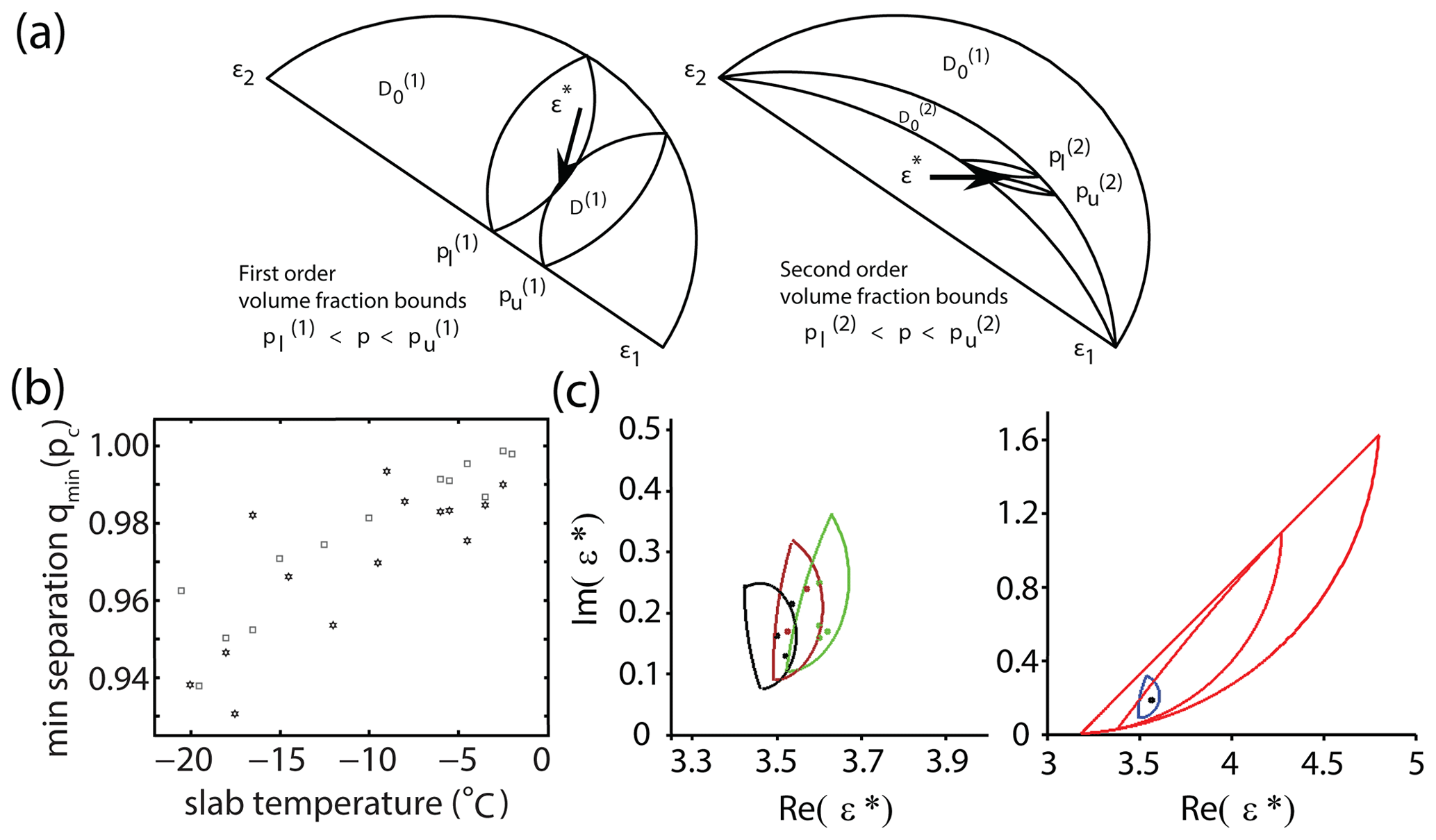
Figure 7Forward and inverse bounds. (a) Illustration of bounds on the volume fraction of one component in the mixture derived from first-order anisotropic bounds (left panel), and from the second-order isotropic bounds (right panel) for the effective permittivity (Cherkaev and Golden, 1998). The small lens-shaped domains each contain ϵ* of the anisotropic (left) and isotropic (right) composites corresponding to the volume fractions of the first component pl and pu which give the lower and upper bounds for the fraction of the first material. (b) Lower bounds on the separation parameter qmin versus temperature (Orum et al., 2012) calculated using data on the effective complex permittivity. The inverted data clearly indicate that as the ice warms, the separations of the brine inclusions decrease. Stars and squares indicate different sea ice slabs. (c) Polycrystalline bounds for different brine volume fractions (Gully et al., 2015) for the permittivity of sea ice (left) together with the measured effective permittivity of sea ice in (Arcone et al., 1986). Comparison between two-component and polycrystalline bounds (right) – the forward polycrystalline bounds shown in blue are a dramatic improvement over the two-component forward elementary bounds and isotropic bounds shown in red.
First- and second-order forward and inverse bounds are illustrated in Fig. 7a (Cherkaev and Golden, 1998), where first-order bounds for the effective complex permittivity of all anisotropic composites that could be formed from two materials of permittivity ϵ1 and ϵ2 are presented in the left panel, while the second-order isotropic bounds are shown in the right panel. The small lens shaped domains each contain the anisotropic (left) and isotropic (right) mixtures corresponding to the volume fractions ϕ of the first component equal to and , . The points and give the lower and upper bounds for the volume fraction of the first material in the composite. Superscripts q=1 and q=2 indicate the first- and second-order bounds. For a set of data points ϵ*(k), corresponding to composites with the same structure, the bounds for the fraction ϕ of the first phase in the material are given by an intersection of all admissible intervals (Cherkaev and Tripp, 1996):
Here, and are lower and upper bounds for the volume fraction ϕ calculated using the effective complex permittivity ϵ∗(k), respectively, and q is the order of the bounds, with q=1 for a general mixture and q=2 for an isotropic composite.
In Cherkaev and Golden (1998), this method was applied to estimating brine volume fraction in sea ice from two data sets of 4.75 GHz measurements of the complex permittivity ϵ* of sea ice (Arcone et al., 1986) at −6 and −11 ∘C with fractions of brine ϕ=0.036 and ϕ=0.0205. Sea ice was considered a composite of three components: pure ice, brine, and air. The effective complex permittivity of the mixture of ice and air was calculated with the Maxwell–Garnett formula. The first-order bounds estimate the brine volume fraction as and , for the data set 1 and 2, respectively. The second-order inverse bounds derived with the assumption of 2D isotropy in the horizontal plane give the following estimates for the brine volume fraction: for the first data set with brine volume ϕ=0.036 and for the second data set with volume fraction of brine ϕ=0.0205. The first-order bounds are further extended to polycrystalline materials and allow estimation of the mean crystal orientation (Gully et al., 2015).
5.2 Matrix-particle forward and inverse bounds
Another parameter important in characterizing the structure of a composite material consisting of inclusions within a host matrix is the separation between inclusions. Inclusion separation is an indicator of the connectedness of phases – a key feature in critical behavior and phase transitions; the separation parameter may be used to estimate closeness to the percolation phase transition.
Composites with non-touching inclusions of one material embedded in a host matrix of a different material are called matrix-particle composites (Bruno, 1991). For a matrix-particle composite with separated inclusions, tighter bounds on the effective complex permittivity may be obtained. In Orum et al. (2012), sea ice is considered a matrix-particle composite in which the brine phase is contained in separated, circular discs of radii rb randomly located on a horizontal plane, each surrounded by a “corona” of ice with outer radius ri. Such a material is called a q material, where . The minimal separation of brine inclusions is . In this case, as it is shown in Bruno (1991), the support of μ in Eq. (5) lies in an interval [sm,sM], such that and . The further the separation of the inclusions, the smaller the interval [sm,sM], and the tighter the bounds. Smaller q values indicate well-separated brine (and colder temperatures as in Fig. 7), while q=1 corresponds to no restriction on the separation, with sm=0 and sM=1.
Two parameters characterizing the structure of the sea ice composite are the volume fraction ϕ of the brine inclusions and a separation parameter q that quantifies how close the inclusions are to each other. Using observed values of effective complex permittivity and inverting the forward-matrix-particle bounds, information about these two parameters is obtained in Orum et al. (2012) by solving a reduced inverse spectral problem and bounding the volume fraction of the constituents. Inverse bounds for inclusion separation are shown in Fig. 7 (Orum et al., 2012), where the lower bound qmin is displayed versus temperature of the sea ice slab. The inverted data clearly indicate that as the ice warms, the separations of the brine inclusions decrease. It is remarkable that this important phenomenon is characterized from electromagnetic measurements through an inversion scheme.
5.3 Extension to polycrystalline composites
The method of inverse bounds (Cherkaev and Tripp, 1996; Cherkaev and Golden, 1998; Tripp et al., 1998) for structural parameters of a composite from measured effective properties was extended to polycrystalline materials in Gully et al. (2015). In the case of a uniaxial polycrystalline composite, Gully et al. (2015) developed bounds for the mean orientation of crystals in the sea ice from measured values of ice permittivity. As columnar and granular microstructures have different mean single crystal orientations (Weeks and Ackley, 1982), this inverse approach is useful for determining ice type when using remote sensing techniques.
The structures of different types of ice formed under different environmental conditions vary tremendously. For instance, for congelation ice frozen under calm conditions, the crystals are vertically elongated columns, and each crystal itself is a composite of pure ice platelets separating layers of brine inclusions. The orientation of each individual crystallite is determined by the direction of the c axis, which is perpendicular to the orientation of platelets or lamellae of pure ice. Finding the bounds for the crystal orientations enables us to electromagnetically distinguish columnar ice from granular ice. This is a critical problem in sea ice physics and biology, as these different structures have vastly different fluid flow properties, which affects melt pond evolution, nutrient replenishment, brine convection, and other mesoscale processes in the ice cover.
Bounds for the effective permittivity of polycrystalline composites are much tighter than those bounding the permittivity of a general two-component material. Such polycrystalline bounds constructed in Gully et al. (2015) are shown in Fig. 7c. This dramatic improvement over the classic two-component bounds is due to additional information about single crystal orientations included in the new bounds.
As was discussed in the polycrystal section, the zeroth moment in Eq. (16) of the measure μ in the integral representation of the effective properties of a uniaxial polycrystalline material is , where the statistical average can be viewed as the “mean crystal orientation” related to the percentage of crystallites oriented in the kth direction. Extending the inverse bounds method (Cherkaev and Tripp, 1996; Cherkaev and Golden, 1998; Tripp et al., 1998) to polycrystalline materials, the inverse polycrystalline bounds (Gully et al., 2015) estimate the mean crystal orientation by bounding the zeroth moment of the measure μ using measured data on the ice permittivity. This procedure gives an analytic estimate (the first-order inverse bounds) for the range of values of the mean crystal orientation similar to Eq. (23):
Here, X1 is defined in the polycrystalline section as X1=RTCR; f is the known value of F(s); and g is the known value of , with .
Inverse polycrystalline bounds computed in Gully et al. (2015) for different types of sea ice, granular and columnar, show that the method allows the type of ice to be revealed through electromagnetic data. For statistically isotropic granular ice shown in Fig. 6a (top), the inverse mean crystal orientation bounds (Gully et al., 2015) estimate the deviation angle as (with the true value ). The inverse mean crystal orientation bounds (Gully et al., 2015) for columnar ice (see Fig. 6a, bottom) estimate the angle of deviation of the crystal's axis from the vertical as 20±8∘. These results demonstrate a significant difference in the reconstructed mean orientations of crystals in columnar and in granular ice and provide a foundation for distinguishing the types of ice using electromagnetic measurements.
The enhancement of diffusive transport of passive scalars by complex fluid flow plays a key role in many important processes in the global climate system (Washington and Parkinson, 1986) and Earth's ecosystems (Di Lorenzo et al., 2013). Advection of geophysical fluids intensifies the dispersion and large-scale transport of heat (Moffatt, 1983), pollutants (Csanady, 1963; Beychok, 1994; Samson, 1988), and nutrients (Di Lorenzo et al., 2013; Hofmann and Murphy, 2004) diffusing in their environment. In sea ice dynamics, where the ice cover couples the atmosphere to the polar oceans (Washington and Parkinson, 1986), the transport of sea ice can also be enhanced by eddy fluxes and large-scale coherent structures in the ocean (Watanabe and Hasumi, 2009; Lukovich et al., 2015). In sea ice thermodynamics, the temperature field of the atmosphere is coupled to the temperature field of the ocean through sea ice, a composite of pure ice with brine inclusions whose volume fraction and connectedness depend strongly on temperature (Thomas and Dieckmann, 2003; Golden et al., 2007; Golden, 2009). Convective brine flow through the porous microstructure can enhance thermal transport through the sea ice layer (Lytle and Ackley, 1996; Worster and Jones, 2015).
Over the years, a broad range of mathematical techniques have been developed that reduce the analysis of complex composite materials with rapidly varying structures in space to solving averaged or homogenized equations that do not have rapidly varying coefficients and involve an effective parameter. The core idea here is that the motion of a particle diffusing in a velocity field with regular geometry (including stationary random, periodic, or quasiperiodic variations) is governed on a large-scale and long times by a diffusion equation with an effective diffusion tensor, which depends on the geometry of the velocity field and the local diffusivity. In Taylor (1921), it was first shown that a long-time, large-scale dispersion of passive scalars can be described by an effective diffusivity tensor κ*. Motivated by Papanicolaou and Varadhan (1982), the effective parameter problem was extended to complex velocity fields, with rapidly varying structures in both space and time, providing a rigorous mathematical foundation for calculating effective (eddy) viscosity and the effective (eddy) diffusivity tensors (McLaughlin et al., 1985). The effective parameter problem of (anomalous) super-diffusion and sub-diffusion is given in Biferale et al. (1995) and Fannjiang (2000). Based on McLaughlin et al. (1985), Avellaneda and Majda (1989, 1991) adapted the ACM (Golden and Papanicolaou, 1983) to the advection diffusion equation and obtained a Stieltjes integral representation of the effective diffusivity tensor κ* for flows with zero mean drift involving the Péclet number ξ of the flow. This representation encapsulates the geometric complexity of the flow in a spectral measure associated with a random Hermitian operator (or matrix). Using methods developed for composite media (Milton, 2002), they obtained rigorous bounds on the components of κ*. Moreover, in analogy to methods developed for composites (Milton, 2002), they also found velocity fields which realize these bounds, such as the famous confocal sphere configurations that realize the Hashin–Shtrikman bounds of composites (Hashin and Shtrikman, 1962; Avellaneda and Majda, 1991). Remarkably, this method has also been extended to time-dependent flows (Avellaneda and Vergassola, 1995; Murphy et al., 2017b); flows with incompressible nonzero effective drift (Pavliotis, 2002; Fannjiang and Papanicolaou, 1994); flows where particles diffuse according to linear collisions (Pavliotis, 2010); and solute transport in porous media (Bhattacharya, 1999), which has a direct application to diffusive brine advection in sea ice. All yield Stieltjes integral representations of the symmetric and, when appropriate, the antisymmetric part of κ*.
We now briefly describe our recent results on this framework (Murphy et al., 2017b, 2020a). It is an important example of how Stieltjes integral representations can provide a rigorous basis for analysis of problems for sea ice involving advection diffusion processes. The dispersion of a cloud of passive scalars with density ϕ(t,x) (not to be confused with earlier usage as the brine volume fraction) diffusing with molecular diffusivity ε and being advected by an incompressible velocity field u(t,x) satisfying is described by the advection–diffusion equation as follows:
Here, the initial density ϕ0(x) and the fluid velocity field u are assumed to be given. In Eq. (26), the molecular diffusion constant is ε>0, and is the Laplacian. This equation also models the transport of heat advected by the fluid velocity field u and diffused with molecular diffusion coefficient ε. To simplify our presentation, we assume that the velocity field u in Eq. (26) is temporally and spatially periodic. Non-dimensionalization (Murphy et al., 2020a) and homogenization (McLaughlin et al., 1985) of Eq. (26) shows that long-time, large-volume (or area) macroscopic thermal transport is described by a diffusion equation involving an averaged scalar density and a symmetric, constant (Pavliotis, 2002) effective diffusivity tensor κ* (McLaughlin et al., 1985),
For simplicity, we consider a diagonal coefficient , , of κ*; set ; and write u=u0v, where u0 is the (constant) strength of u and v is a non-dimensional velocity field containing the geometric and dynamic information about u. In these non-dimensional variables, the Péclet number ξ and molecular diffusivity ε are related by (Murphy et al., 2017b, 2020a).
Using a mathematical framework that is strikingly similar to that in Sect. 3, the effective diffusivity has the following Stieltjes integral representation (McLaughlin et al., 1985; Avellaneda and Majda, 1991; Murphy et al., 2017b, 2020a):
where 〈⋅〉 denotes averaging over the space–time period cell for periodic flows (Murphy et al., 2017b, 2020a) or statistical average for random flows (Avellaneda and Majda, 1989; Avellaneda and Vergassola, 1995), and ψk is the solution to a cell problem (McLaughlin et al., 1985; Murphy et al., 2017b). An equivalent statement which emphasizes the connection to the two-component composites setting in Eq. (5) is
The vector field satisfies Eq. (3) for two-component composite materials, with D=ϵE, , , and ϵ plays the role of the medium's electrical permittivity tensor (Murphy et al., 2017b, 2020a). Here, ∂t denotes partial differentiation with respect to time, and H(t,x) is the stream matrix, given in terms of the incompressible velocity field , that satisfies (Avellaneda and Majda, 1991, 1989). When the flow is time-independent, v=v(x), then ψk=ψk(x) and S=H(x). Moreover , with defined above (Murphy et al., 2017b). The integral representation for κ* in Eq. (28) follows from the resolvent formula
which is an analogue of Eq. (6). The operator ΓSΓ is antisymmetric due to the asymmetry of both the operators ∂t and H, so iΓSΓ is a self-adjoint operator (Murphy et al., 2017b), where is the imaginary unit, and is the same projection operator arising in the setting of two-component composites. Equation (28) shows that brine advection enhances the thermal diffusivity since .
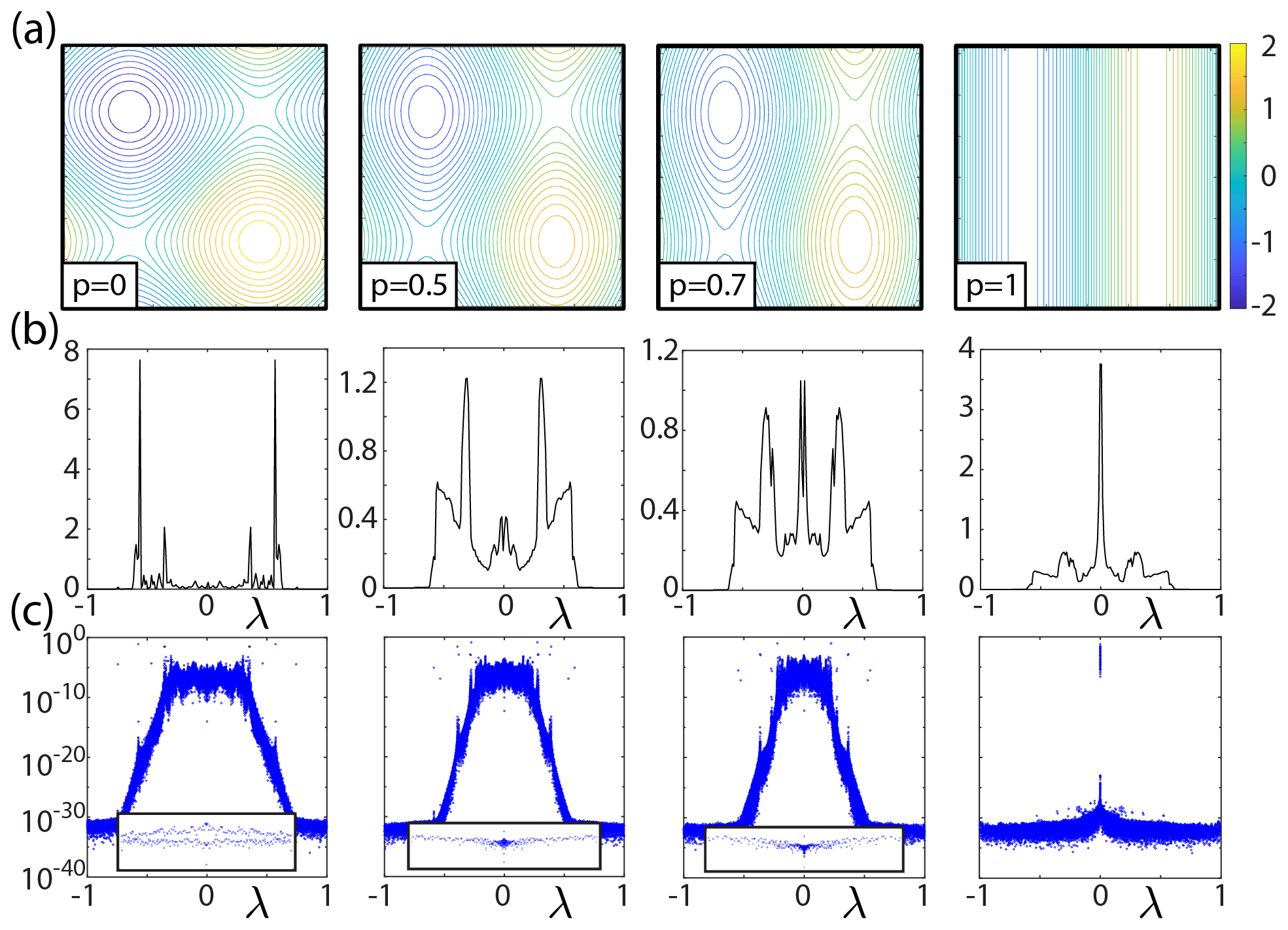
Figure 8Spectral measures for effective diffusivities. (a) Streamlines for BC flow with fluid velocity field with B=1, , and increasing values of p from left to right. BC cell flow with closed streamlines arises for . As the value of C decreases from 1, the streamlines elongate in the y direction giving rise to large-scale thermal transport, even in the absence of molecular diffusivity, when ε=0. BC shear flow is attained when B=1 and C=0, for which the spectral measure is known to be a δ function at the origin λ=0 (Avellaneda and Majda, 1991), as shown in the rightmost panel of (a) and (c). (b) Corresponding spectral functions ν22(λ) (histogram representations) for the spectral measures ν22 in (c), which display the spectral measure weights vs. eigenvalues λj of the matrix M=iΓHΓ for the value of p shown in (a). Since the streamlines do not become elongated in the x direction, the spectral functions for the measure ν11 are qualitatively similar to those of ν22 for BC cell flow, for all p. The spectral functions in (b) are ensemble averaged for B=1 and with , with p=0.01, 0.5, 0.7, and 1, from left to right. The zoomed-in insets in (c) with show the density of the measure near the spectral origin λ=0 increasing as BC cell flow transitions to BC shear flow.
Analytical calculations of the spectral measure ν are extremely difficult except for simple flows like shear flow (Avellaneda and Majda, 1991). However, Padé approximants provide rigorous, converging upper and lower bounds (Baker and Graves-Morris, 1996) for the Stieltjes function in Eqs. (28) and (29), where ; Padé approximants can be calculated using the moments νn of ν. Despite this, the lack of a method to calculate the moments νn of ν has impeded progress on obtaining explicit bounds for specific flows using this procedure (Avellaneda and Majda, 1991, 1989) since 1991. We have recently developed a mathematical framework that can be used to compute, in principle, all of the moments νn for a spatially or space–time periodic velocity field v, hence Padé approximant bounds. We have utilized these results to provide rigorous bounds for the enhancement of sea ice thermal conductivity by brine fluid velocity fields. These findings will be published elsewhere.
Spectral measure computations for advection diffusion processes
We have extended our numerical methods discussed for two-component media in Sect. 3.1 to compute the spectral measure ν for spatially periodic flows (Murphy et al., 2020a) and developed Fourier methods for computing ν for space-time periodic flows (Murphy et al., 2017b). For simplicity, we focus our discussion to the setting of spatially periodic flows. Computing the spectral measure ν for a given flow involves discretizing the spatially dependent stream matrix H(x), which becomes a banded antisymmetric matrix satisfying . The projection matrix Γ is given by that in Sect. 3.1, and the key self-adjoint operator is given by G=iΓHΓ, which becomes a Hermitian matrix M. In this case, the integral in Eq. (28) and the resolvent in Eq. (30) are given in terms of the eigenvalues λj and eigenvectors wj of the matrix M
which is analogous to Eq. (9).
The computations in Murphy et al. (2017b, 2020a) and those displayed in Fig. 8 show that the spectral origin λ=0 for advection diffusion plays the role of the spectral endpoints for two-component and polycrystalline composite materials. An increase in spectral mass at λ=0 increases the advection-driven enhancement of effective diffusivity above the bare molecular diffusivity ε in the advection-dominated regime, where ε≪1 (or Péclet number ξ≫1). For example, the closed streamlines shown in the leftmost panel of Fig. 8a for BC cell flow, with fluid velocity field and , transport tracers in a short-range periodic motion, so long-range transport is only possible due to molecular diffusion. Consequently, in the advection-dominated regime, the effective diffusivity scales as (Fannjiang and Papanicolaou, 1994, 1997; Murphy et al., 2020a), vanishing as ε→0. As shown in Fig. 8b and c, and also in Murphy et al. (2017b, 2020a), this is reflected in the spectral measure ν by the lack of adequate mass near λ=0 for the singular integrand to overcome the multiplicative factor of ε for in Eq. (28).
On the other hand, when B≠C the streamlines elongate and connect to neighboring cells which gives rise to long-range advection of tracers, even in the absence of molecular diffusion. This is reflected in the spectral measure by a buildup of adequate mass near λ=0 for the singular integrand to overcome the multiplicative factor of ε for in Eq. (28), leading to a non-zero value of κ* in the limit ε→0 (Murphy et al., 2017b). This is a key example of how the behavior of the spectral measure ν governs the behavior of the bulk transport coefficient κ*.
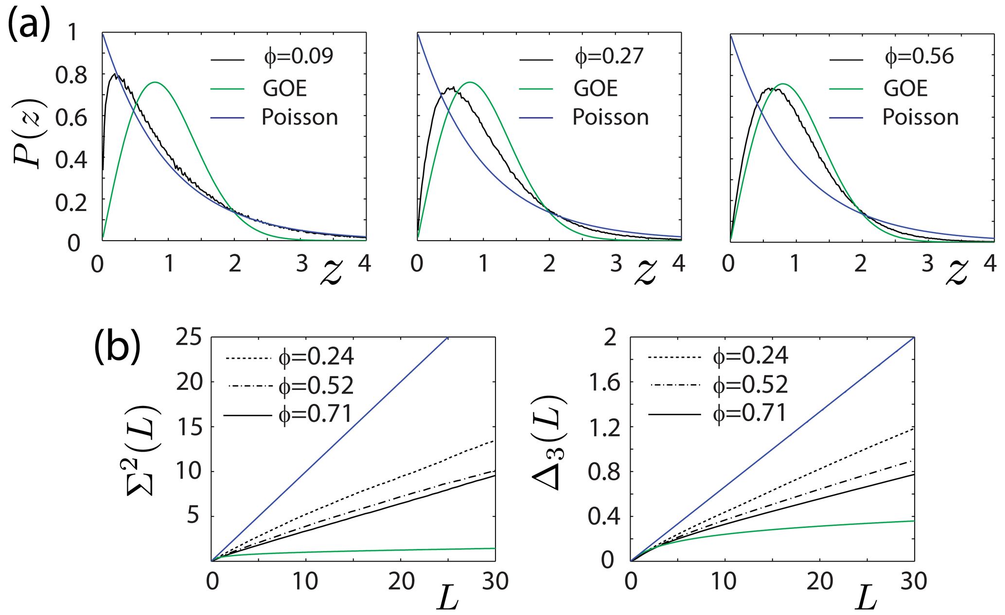
Figure 9Eigenvalue spacing statistics for sea ice melt ponds (a) and long-range eigenvalue statistics for the brine structures in sea ice (b). (a) Eigenvalue spacing distribution (ESD) P(z) for the melt ponds shown in Fig. 4. (b) Spectral statistics for the brine structures shown in Fig. 3. We see the transition toward universal Wigner–Dyson statistics as melt water phases and brine phases become connected over the scale of the sample.
In random matrix theory (RMT) (Guhr et al., 1998; Bohigas and Giannoni, 1984; Deift and Gioev, 2009), long- and short-range correlations of the bulk eigenvalues away from the spectral edge (Canali, 1996; Guhr et al., 1998) for random matrices are measured using various eigenvalue statistics (Guhr et al., 1998; Bohigas and Giannoni, 1984), such as the eigenvalue spacing distribution (ESD), spectral rigidity Δ3, and number variance Σ2. To observe statistical fluctuations of these bulk eigenvalues about the mean density, the eigenvalues must be unfolded (Bohigas and Giannoni, 1984; Guhr et al., 1998; Canali, 1996; Plerou et al., 2002). The localization properties of the eigenvectors are measured in terms of quantities such as the inverse participation ratio (IPR) (Plerou et al., 2002; Evers and Mirlin, 2008).
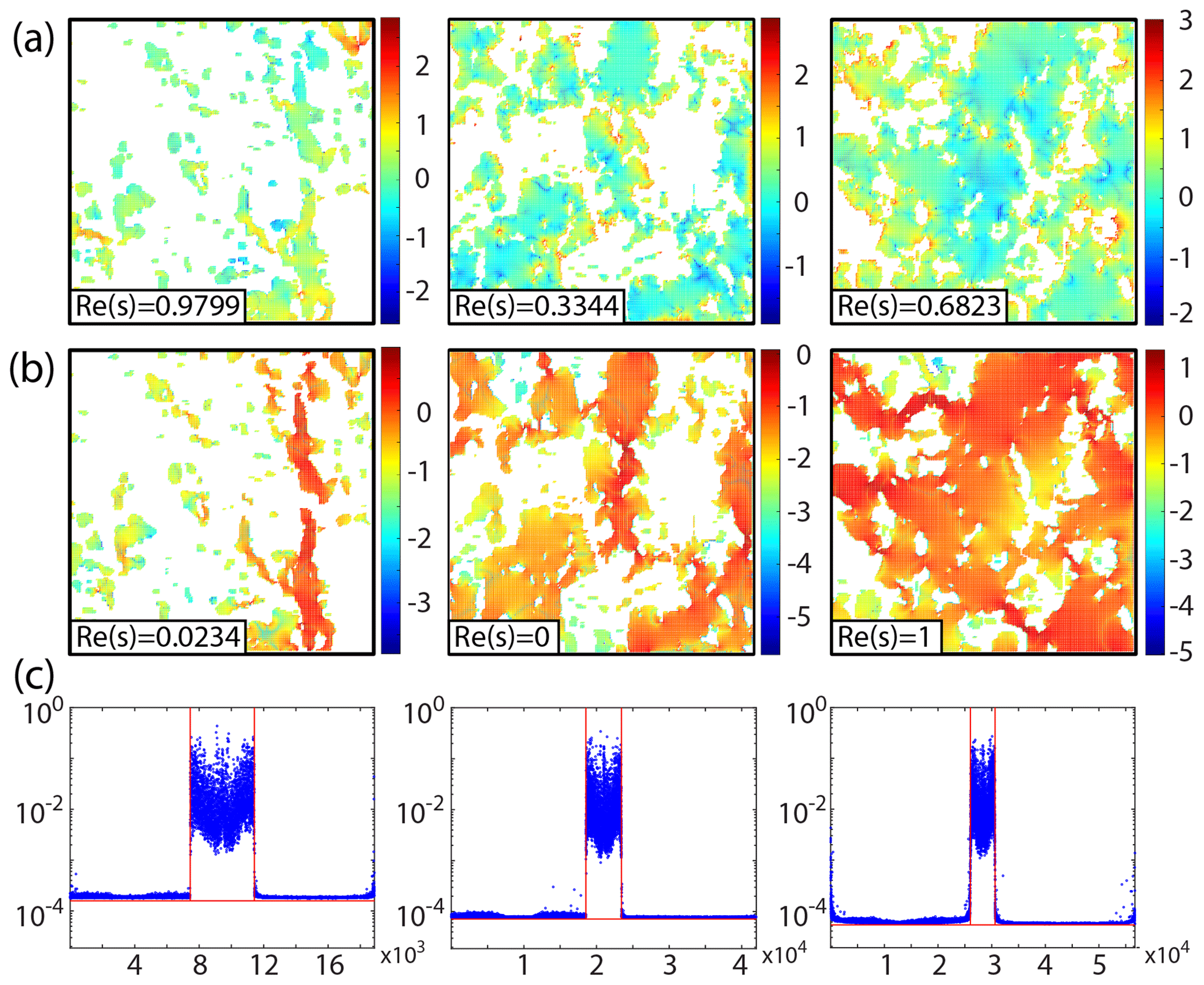
Figure 10Anderson localization transition for electric fields in sea ice brine microstructure. Examples of (a) localized and (b) extended electric fields for sea ice brine microstructure with increasing connectedness from left to right. The values of s are taken to satisfy Im(s)=0.001 with . The electric fields are displayed for values of Re(s) which (a) maximize and (b) minimize IPR[E](s), which correspond to the values of such s associated with (a) most localized and (b) most extended electric fields. (c) Corresponding IPR for eigenvectors wj plotted versus index j. The vertical lines define the δ components of μ, where the eigenvalues satisfy and . The horizontal lines mark the IPR value for the Gaussian orthogonal ensemble (GOE) with matrix size N1≈ϕN, where N=Ldd.
In Murphy et al. (2017a), we found that as a percolation threshold is approached and long-range order develops, the behavior of the ESD transitions from weakly correlated Poissonian statistics toward obeying universal Wigner–Dyson (WD) statistics of the Gaussian orthogonal ensemble (GOE). The eigenvectors de-localize, and mobility edges appear (Murphy et al., 2017a), similar to the metal/insulator transition in solid state physics. We explored the transition in the 2D and 3D RRN, as well as in sea ice microstructures such as in 2D discretizations of the brine microstructure of sea ice (Golden et al., 1998a, 2007; Golden, 2009), melt ponds on Arctic sea ice (Hohenegger et al., 2012), the sea ice pack itself, and porous human bone (Golden et al., 2011; Kabel et al., 1999; Bonifasi-Lista and Cherkaev, 2009; Cherkaev and Bonifasi-Lista, 2011). We extended these results to two-component composite media with quasiperiodic microgeometry in Morison et al. (2022).
For highly correlated WD spectra exhibited by, for example, real-symmetric matrices of the GOE, the nearest-neighbor ESD P(z) is accurately approximated by , which illustrates eigenvalue repulsion and vanishes linearly as spacings z→0 (Guhr et al., 1998; Stone et al., 1991; Canali, 1996). In contrast, the ESD for uncorrelated Poisson spectra, , allows for significant level degeneracy (Guhr et al., 1998). In Fig. 9a we display the ESDs for Poisson (blue) and WD (green) spectra, along with the behavior of the ESDs for the matrix M=χ1Γχ1, corresponding to the Arctic melt ponds in Fig. 4 with fluid area fraction ϕ. It shows that for sparsely connected systems, the behavior of the ESDs is well described by weakly correlated Poisson-like statistics (Canali, 1996). With increasing connectedness, the ESDs transition toward highly correlated WD statistics with strong level repulsion. This behavior of the ESD reveals a mechanism for the collapse in the spectral gaps of μ. For sparsely connected systems, the weak level repulsion allows for significant level degeneracy and resonances in μ as shown in Murphy et al. (2015) for the 2D percolation model and in Fig. 4a for Arctic melt pond microstructure. As the system becomes increasingly connected, the level repulsion increases, causing the eigenvalues to spread out, which, in turn, causes the gaps in the measure near the spectral edges to collapse and subsequently form δ components of the measure at the spectral endpoints (as shown in the figures in Sect. 3.1). Our computations of Δ3 and Σ2 are shown in Fig. 9b for the brine microstructure in Fig. 3. Notice that as the system becomes increasingly connected, the long-range statistics transition towards that of the GOE, indicating an increase in the long-range correlations of the eigenvalues.
The eigenvectors wj of M=χ1Γχ1, associated with the N1×N1 submatrices of Γ, also exhibit a connectedness-driven transition in their localization properties. The IPR is defined as , , where is the ith component of wj. Eigenvectors of matrices in the GOE are known to be highly extended (Deift and Gioev, 2009), with an asymptotic value of the IPR given by (Plerou et al., 2002).
In Murphy et al. (2017a), we found for the 2D and 3D percolation models that as p surpasses pc and long-range order is established in a RRN, “mobility edges” form in the eigenvector IPR, with a sudden increase in the number of extended eigenvectors. This is analogous to Anderson localization, where mobility edges mark the characteristic energies of the metal–insulator transition (MIT) (Guhr et al., 1998). Remarkably, the mobility edges for RRN are due to very extended eigenstates associated with δ components that form at the spectral endpoints precisely at the percolation threshold pc (and 1−pc for 3D) (Murphy and Golden, 2012), which control critical behavior in insulator/conductor and conductor/superconductor systems (Murphy and Golden, 2012; Clerc et al., 1990; Bergman and Stroud, 1992). This and other eigenvector phenomena were observed for two-component composite media with quasiperiodic microgeometry in Morison et al. (2022).
The IPR phenomenon for the eigenvectors of the matrix M=χ1Γχ1 is shown for sea ice brine microstructure in Fig. 10c. The electric field E within sea ice brine microstructure exhibits a frequency-dependent Anderson localization transition, as shown in Fig. 10a and b. To generate these figures, the IPR of the electric field, IPR[E](s) in the brine phase χ1E, was calculated as a function of s via Eq. (9) for Im s=0.001 and and then normalized to have unit length. The values of s were then selected where IPR[E](s) attains its maximum and minimum, corresponding to the most localized and most extended E, respectively. For those values of s, the electric fields for brine microstructure are shown in Fig. 10a and b. The localized electric fields in (a) are characterized by high-intensity “hot spots” at the brine-ice interfaces, while extended electric fields have high intensities spread out more evenly across the connected and near-connected brine components.
We have gone on a tour of various areas of sea ice physics concerned with homogenization and how they can be rigorously addressed with the powerful analytic continuation method and its extensions. The effective complex permittivity of sea ice treated as a two-phase composite of pure ice with brine inclusions, or treated as a polycrystalline material, and the effective diffusivity for advection diffusion problems are all Stieltjes functions of their variables. We showed how these functions have integral representations involving spectral measures which distill the mixture or velocity field geometries into the spectral properties of a self adjoint operator, akin to the Hamiltonian in quantum physics. These spectral representations have been used to obtain rigorous forward and inverse bounds on effective transport coefficients for sea ice. Finally, viewing the behavior of these spectral representations through the lens of random matrix theory has revealed fascinating parallels between quantum transport in disordered media, Anderson localization, and classical transport phenomena.
This work exclusively uses software that is currently in development by the authors and has not yet been made publicly available. The data used in the numerical results and the creation of figures are available from the corresponding author upon reasonable request.
All authors contributed to planning the work and writing and editing the manuscript.
The contact author has declared that none of the authors has any competing interests.
Publisher's note: Copernicus Publications remains neutral with regard to jurisdictional claims in published maps and institutional affiliations.
This article is part of the special issue “Interdisciplinary perspectives on climate sciences – highlighting past and current scientific achievements”. It is not associated with a conference.
We gratefully acknowledge support from the Applied and Computational Analysis Program and the Arctic and Global Prediction Program at the US Office of Naval Research (grant nos. N00014-18-1-2552, N00014-21-1-2909, N00014-13-10291, N00014-15-1-2455, and N00014-18-1-2041). We are also grateful for support from the Division of Mathematical Sciences and the Division of Polar Programs at the US National Science Foundation (NSF) (grant nos. DMS-0940249, DMS-2136198, DMS-2111117, DMS-2206171, DMS-1715680, and DMS-1413454). Finally, we would like to thank the NSF Math Climate Research Network (MCRN), and especially Chris Jones, for supporting this work.
This research has been supported by the Office of Naval Research (grant nos. N00014-21-1-2909, N00014-18-1-2552, N00014-13-10291, N00014-15-1-2455, and N00014-18-1-2041) and the National Science Foundation (grant nos. DMS-2206171, DMS-2111117, DMS-0940249, DMS-2136198, DMS-1715680, and DMS-1413454).
This paper was edited by Vera Melinda Galfi and reviewed by two anonymous referees.
Anderson, P.: Absence of diffusion in certain random lattices, Phys. Rev., 109, 1492–1505, 1958. a
Arcone, S. A., Gow, A. J., and McGrew, S.: Structure and dielectric properties at 4.8 and 9.5 GHz of saline ice, J. Geophys. Res., 91, 14281–14303, 1986. a, b, c
Avellaneda, M. and Majda, A.: Stieltjes integral representation and effective diffusivity bounds for turbulent transport, Phys. Rev. Lett., 62, 753–755, 1989. a, b, c, d, e, f
Avellaneda, M. and Majda, A.: An integral representation and bounds on the effective diffusivity in passive advection by laminar and turbulent flow, Comm. Math. Phys., 138, 339–391, 1991. a, b, c, d, e, f, g, h, i
Avellaneda, M. and Vergassola, M.: Stieltjes integral representation of effective diffusivities in time-dependent flows, Phys. Rev. E, 52, 3249–3251, 1995. a, b
Backstrom, L. G. E. and Eicken, H.: Capacitance probe measurements of brine volume and bulk salinity in first-year sea ice, Cold Reg. Sci. Technol., 46, 167–180, https://doi.org/10.1016/j.coldregions.2006.08.018, 2006. a
Baker, G. A.: Quantitative Theory of Critical Phenomena, Academic Press, New York, https://doi.org/10.1016/B978-0-12-075120-4.X5001-5, 1990. a
Baker, G. A. and Graves-Morris, P. R.: Padé Approximants, Encyclopedia of Mathematics and its Applications, Cambridge University Press, 746 pp., ISBN 0521450071, 9780521450072, 1996. a, b
Banwell, A., Burton, J., Cenedese, C., Golden, K. M., and Åström, J.: Physics of the cryosphere, Nature Rev. Phys., 5, 446–449, 2023. a
Barabash, S. and Stroud, D.: Spectral representation for the effective macroscopic response of a polycrystal: application to third-order non-linear susceptibility, J. Phys. Condens. Matter, 11, 10323–10334, 1999. a, b
Bates, H. F. and Shapiro, L. H.: Long-period gravity waves in ice-covered sea, J. Geophys. Res., 85, 1095, https://doi.org/10.1029/jc085ic02p01095, 1980. a
Bensoussan, A., Lions, J. L., and Papanicolaou, G.: Asymptotic Analysis for Periodic Structures, North-Holland, Amsterdam, the Netherlands, ISBN 9780080875262, 1978. a
Bergman, D. J.: The dielectric constant of a composite material – A problem in classical physics, Phys. Rep. C, 43, 377–407, 1978. a, b
Bergman, D. J.: Exactly solvable microscopic geometries and rigorous bounds for the complex dielectric constant of a two-component composite material, Phys. Rev. Lett., 44, 1285–1287, 1980. a, b, c, d, e
Bergman, D. J.: Rigorous bounds for the complex dielectric constant of a two–component composite, Ann. Phys., 138, 3058–3065, 1982. a, b, c
Bergman, D. J.: Eigenstates of Maxwell's equations in multiconstituent microstructures, Phys. Rev. A, 105, 062213, https://doi.org/10.1103/PhysRevA.105.062213, 2022. a
Bergman, D. J. and Stroud, D.: Physical properties of macroscopically inhomogeneous media, Solid State Phys., 46, 147–269, 1992. a, b, c
Bergman, D. J., Chen, P. Y., and Farhi, A.: Scattering electromagnetic eigenstates of a two-constituent composite and their exploitation for calculating a physical field, Phys. Rev. A, 102, 063508, https://doi.org/10.1103/PhysRevA.102.063508, 2020. a
Beychok, M. R.: Fundamentals of Stack Gas Dispersion, self-published, 193 pp., ISBN 0964458802, 9780964458802, 1994. a
Bhattacharya, R.: Multiscale diffusion processes with periodic coefficients and an application to solute transport in porous media, Ann. Appl. Probab., 9, 951–1020, 1999. a
Bi, C., Ou, M.-J. Y., and Zhang, S.: Integral representation of hydraulic permeability, P. Royal Soc. Edinburgh A, 153, 907–936, https://doi.org/10.1017/prm.2022.25, 2023. a
Biferale, L., Crisanti, A., Vergassola, M., and Vulpiani, A.: Eddy diffusivities in scalar transport, Phys. Fluids, 7, 2725–2734, 1995. a, b
Bohigas, O. and Giannoni, M. J.: Chaotic motion and random matrix theories, in: Mathematical and computational methods in nuclear physics (Granada, 1983), vol. 209 of Lecture Notes in Physics, Springer, Berlin, 1–99, https://doi.org/10.1007/3-540-13392-5_1, 1984. a, b, c
Bonifasi-Lista, C. and Cherkaev, E.: Analytical relations between effective material properties and microporosity: Application to bone mechanics, Int. J. Eng. Sci., 46, 1239–1252, 2008. a, b, c, d
Bonifasi-Lista, C. and Cherkaev, E.: Electrical impedance spectroscopy as a potential tool for recovering bone porosity, Phys. Med. Biol., 54, 3063–3082, 2009. a, b, c, d, e, f, g
Bonifasi-Lista, C., Cherkaev, E., and Yeni, Y. N.: Analytical approach to recovering bone porosity from effective complex shear modulus, J. Biomech. Eng., 131, 121003, https://doi.org/10.1115/1.4000082, 2009. a, b, c, d
Broadbent, S. R. and Hammersley, J. M.: Percolation processes I. Crystals and mazes, Proc. Cambridge Philos. Soc., 53, 629–641, 1957. a, b
Bruno, O.: The effective conductivity of strongly heterogeneous composites, Proc. R. Soc. London A, 433, 353–381, 1991. a, b, c
Bunde, A. and Havlin, S. (Eds.): Fractals and Disordered Systems, Springer-Verlag, New York, https://doi.org/10.1007/978-3-642-51435-7, 1991. a, b
Canali, C. M.: Model For a random-matrix description of the energy-level statistics of disordered systems at the Anderson transition, Phys. Rev. B, 53, 3713–3730, 1996. a, b, c, d
Chayes, J. T. and Chayes, L.: Bulk transport properties and exponent inequalities for random resistor and flow networks, Comm. Math. Phys., 105, 133–152, 1986. a
Cherkaev, E.: Inverse homogenization for evaluation of effective properties of a mixture, Inverse Problems, 17, 1203–1218, 2001. a, b, c, d, e, f, g, h, i, j, k, l, m, n, o, p, q, r, s, t
Cherkaev, E.: Spectral coupling of effective properties of a random mixture, in: IUTAM Symposium on Asymptotics, Singularities and Homogenisation in Problems of Mechanics, edited by: Movchan, A. B., vol. 113 of Solid Mechanics and Its Applications, Springer Netherlands, 331–340, https://doi.org/10.1007/1-4020-2604-8_32, 2004. a, b
Cherkaev, E.: Internal friction and the Stieltjes analytic representation of the effective properties of two-dimensional viscoelastic composites, Arch. Appl. Mech., 89, 591–607, 2019. a, b, c, d, e
Cherkaev, E.: Internal resonances and relaxation memory kernels in composites, Philos. T. Roy. Soc. A, 378, 20190106, https://doi.org/10.1098/rsta.2019.0106, 2020. a, b, c
Cherkaev, E. and Bonifasi-Lista, C.: Characterization of structure and properties of bone by spectral measure method, J. Biomech., 44, 345–351, https://doi.org/10.1016/j.jbiomech.2010.10.031, 2011. a, b, c, d, e, f, g, h, i, j, k, l, m, n
Cherkaev, E. and Golden, K. M.: Inverse bounds for microstructural parameters of composite media derived from complex permittivity measurements, Waves in random media, 8, 437–450, 1998. a, b, c, d, e, f, g, h, i, j, k, l, m, n
Cherkaev, E. and Ou, M.-J.: Dehomogenization: reconstruction of moments of the spectral measure of the composite, Inverse Problems, 24, 065008, https://doi.org/10.1088/0266-5611/24/6/065008, 2008. a, b, c, d
Cherkaev, E. and Tripp, A. C.: Bounds on porosity for dielectric logging, in: 9th Conference of the European Consortium for Mathematics in Industry, 304–306, Technical University of Denmark, Copenhagen, Denmark, 1996. a, b, c, d, e, f, g, h, i, j
Cherkaev, E. and Zhang, D.: Coupling of the effective properties of a random mixture through the reconstructed spectral representation, Physica B, 338, 16–23, 2003. a, b
Christensen, K. and Moloney, N. R.: Complexity and Criticality, Imperial College Press, London, 2005. a
Clerc, J. P., Giraud, G., Laugier, J. M., and Luck, J. M.: The electrical conductivity of binary disordered systems, percolation clusters, fractals and related models, Adv. Phys., 39, 191–309, 1990. a
Csanady, G. T.: Turbulent diffusion of heavy particles in the atmosphere, J. Atmos. Sci., 20, 201–208, https://doi.org/10.1175/1520-0469(1963)020<0201:TDOHPI>2.0.CO;2, 1963. a
Day, A. R. and Thorpe, M. F.: The spectral function of random resistor networks, J. Phys. Cond. Matt., 8, 4389–4409, 1996. a
Day, A. R. and Thorpe, M. F.: The spectral function of composite - the inverse problem., J. Phys. Cond. Matt., 11, 2551–2568, 1999. a, b
Day, A. R., Grant, A. R., Sievers, A. J., and Thorpe, M. F.: Spectral function of composites from reflectivity measurements, Phys. Rev. Lett., 84, 1978–1981, https://doi.org/10.1103/PhysRevLett.84.1978, 2000. a
Deift, P. and Gioev, D.: Random Matrix Theory: Invariant Ensembles and Universality, Courant Lecture Notes, Courant Institute of Mathematical Sciences, 217 pp., ISBN 0821847376, 9780821847374, 2009. a, b
Di Lorenzo, E., Mountain, D., Batchelder, H. P., Bond, N., and Hofmann., E. E.: Advances in marine ecosystem dynamics from US GLOBEC: The horizontal-advection bottom-up forcing paradigm, Oceanography, 26, 22–33, https://doi.org/10.5670/oceanog.2013.73, 2013. a, b
Efros, A. L. and Shklovskii, B. I.: Critical behavior of conductivity and dielectric constant near the metal-non-metal transition threshold, Phys. Stat. Sol. (b), 76, 475–485, 1976. a
Engström, C.: Bounds on the effective tensor and the structural parameters for anisotropic two-phase composite material, J. Phys. D, 38, 3695, https://doi.org/10.1088/0022-3727/38/19/019, 2005. a
Evers, F. and Mirlin, A. D.: Anderson transitions, Rev. Modern Phys., 80, 1355–1418, 2008. a, b
Fannjiang, A. and Papanicolaou, G.: Convection–enhanced diffusion for random flows, J. Stat. Phys., 88, 1033–1076, 1997. a, b
Fannjiang, A. C.: Phase diagram for turbulent transport: sampling drift, eddy diffusivity, and variational principles, Physica D, 136, 145–174, 2000. a
Fannjiang, A. C. and Papanicolaou, G.: Convection enhanced diffusion for periodic flows, SIAM J. Appl. Math., 54, 333–408, 1994. a, b, c
Feng, S., Halperin, B. I., and Sen, P. N.: Transport properties of continuum systems near the percolation threshold, Phys. Rev. B, 35, 197–214, 1987. a
Golden, K.: Bounds on the complex permittivity of sea ice, J. Geophys. Res. (Oceans), 100, 13699–13711, 1995. a, b
Golden, K. and Papanicolaou, G.: Bounds for effective parameters of heterogeneous media by analytic continuation, Comm. Math. Phys., 90, 473–491, 1983. a, b, c, d, e, f, g, h, i, j, k, l, m, n
Golden, K. and Papanicolaou, G.: Bounds for effective parameters of multicomponent media by analytic continuation, J. Stat. Phys., 40, 655–667, 1985. a, b
Golden, K. M.: Bounds on the complex permittivity of a multicomponent material, J. Mech. Phys. Solids, 34, 333–358, 1986. a, b, c, d
Golden, K. M.: Convexity and exponent inequalities for conduction near percolation, Phys. Rev. Lett., 65, 2923–2926, 1990. a
Golden, K. M.: Exponent inequalities for the bulk conductivity of a hierarchical model, Comm. Math. Phys., 43, 467–499, 1992. a, b, c
Golden, K. M.: Percolation models for porous media, in: Homogenization and Porous Media, edited by: Hornung, U., 27–43, Springer-Verlag, 1997a. a, b
Golden, K. M.: The interaction of microwaves with sea ice, in: Wave Propagation in Complex Media, IMA Volumes in Mathematics and its Applications, vol. 96, edited by Papanicolaou, G., 75–94, Springer-Verlag, 1997b. a, b, c, d, e
Golden, K. M.: Critical behavior of transport in lattice and continuum percolation models, Phys. Rev. Lett., 78, 3935–3938, 1997c. a, b, c, d
Golden, K. M.: Climate change and the mathematics of transport in sea ice, Notices of the American Mathematical Society, 56, 562–584 and issue cover, 2009. a, b, c, d, e, f, g, h
Golden, K. M.: Mathematics of sea ice, in: The Princeton Companion to Applied Mathematics, edited by: Higham, N. J., Dennis, M. R., Glendinning, P., Martin, P. A., Santosa, F., and Tanner, J., Princeton University Press, 694–705, https://doi.org/9780691150390, Princeton, 2015. a, b, c
Golden, K. M. and Ackley, S. F.: Modeling of anisotropic electromagnetic reflection from sea ice, J. Geophys. Res.-Oceans, 86, 8107–8116, 1981. a
Golden, K. M., Ackley, S. F., and Lytle, V. I.: The percolation phase transition in sea ice, Science, 282, 2238–2241, 1998a. a, b, c, d, e, f
Golden, K. M., Borup, D., Cheney, M., Cherkaeva, E., Dawson, M. S., Ding, K. H., Fung, A. K., Isaacson, D., Johnson, S. A., , Jordan, A. K., Kong, J. A., Kwok, R., Nghiem, S. V., Onstott, R. G., Sylvester, J., Winebrenner, D. P., and Zabel, I.: Inverse electromagnetic scattering models for sea ice, IEEE T. Geosci. Remote, 36, 1675–1704, 1998b. a, b, c, d
Golden, K. M., Cheney, M., Ding, K. H., Fung, A. K., Grenfell, T. C., Isaacson, D., Kong, J. A., Nghiem, S. V., Sylvester, J., and Winebrenner, D. P.: Forward electromagnetic scattering models for sea ice, IEEE T. Geosci. Remote, 36, 1655–1674, 1998c. a, b, c
Golden, K. M., Eicken, H., Heaton, A. L., Miner, J., Pringle, D., and Zhu, J.: Thermal evolution of permeability and microstructure in sea ice, Geophys. Res. Lett., 34, L16501, https://doi.org/10.1029/2007GL030447, 2007. a, b, c, d, e, f, g
Golden, K. M., Murphy, N. B., and Cherkaev, E.: Spectral analysis and connectivity of porous microstructures in bone, J. Biomech., 44, 337–344, 2011. a, b, c, d, e, f
Golden, K. M., Bennetts, L. G., Cherkaev, E., Eisenman, I., Feltham, D., Horvat, C., Hunke, E., Jones, C., Perovich, D., Ponte-Castañeda, P., Strong, C., Sulsky, D., and Wells, A.: Modeling sea ice, Notices of the American Mathematical Society, 67, 1535–1555, 2020. a, b, c, d
Grimmett, G.: Percolation, Springer-Verlag, New York, 1989. a, b
Guhr, T., Müller-Groeling, A., and Weidenmüller, H. A.: Random-matrix Theories in quantum physics: common concepts, Phys. Rep., 299, 189–425, https://doi.org/10.1016/S0370-1573(97)00088-4, 1998. a, b, c, d, e, f, g, h, i
Gully, A., Backstrom, L. G. E., Eicken, H., and Golden, K. M.: Complex bounds and microstructural recovery from measurements of sea ice permittivity, Physica B, 394, 357–362, 2007. a
Gully, A., Lin, J., Cherkaev, E., and Golden, K. M.: Bounds on the complex permittivity of polycrystalline composites by analytic continuation, P. Roy. Soc. A, 471, 20140702, https://doi.org/10.1098/rspa.2014.0702, 2015. a, b, c, d, e, f, g, h, i, j, k, l, m, n, o, p, q, r, s, t, u, v, w
Halperin, B. I., Feng, S., and Sen, P. N.: Differences between lattice and continuum percolation transport exponents, Phys. Rev. Lett., 54, 2391–2394, 1985. a
Hashin, Z. and Shtrikman, S.: A Variational Approach to the Theory of Effective Magnetic Permeability of Multiphase Materials, J. Appl. Phys., 33, 3125–3131, 1962. a
Hofmann, E. E. and Murphy, E. J.: Advection, krill, and Antarctic marine ecosystems, Antarct. Sci., 16, 487–499, https://doi.org/10.1017/S0954102004002275, 2004. a
Hohenegger, C., Alali, B., Steffen, K. R., Perovich, D. K., and Golden, K. M.: Transition in the fractal geometry of Arctic melt ponds, The Cryosphere, 6, 1157–1162, https://doi.org/10.5194/tc-6-1157-2012, 2012. a, b
Huang, T.-M., Lin, W.-W., and Wang, W.: Matrix representations of discrete differential operators and operations in electromagnetism, Ann. Math. Sci. Appl., 4, 55–79, https://doi.org/10.4310/AMSA.2019.v4.n1.a3, 2019. a
Jonckheere, T. and Luck, J. M.: Dielectric resonances of binary random networks, J. Phys. A, 31, 3687–3717, 1998. a
Kabel, J., Odgaard, A., van Rietbergen, B., and Huiskes, R.: Connectivity and the elastic properties of cancellous bone, Bone, 24, 115–120, 1999. a
Kantor, Y. and Bergman, D. J.: Elastostatic resonances: a new approach to the calculation of the effective elastic constants of composites, J. Mech. Phys. Solids, 30, 355–376, 1982. a, b
Kantor, Y. and Bergman, D. J.: Improved rigorous bounds on the effective elastic moduli of a composite material, J. Mech. Phys. Solids, 32, 41–62, 1984. a
Keller, J. B.: Gravity waves on ice-covered water, J. Geophys. Res.-Oceans, 103, 7663–7669, https://doi.org/10.1029/97jc02966, 1998. a
Kerstein, A. R.: Equivalence of the void percolation problem for overlapping spheres and a network problem, J. Phys. A, 16, 3071–3075, 1983. a
Kozlov, S. M.: Geometric aspects of homogenization, Russ. Math. Surv., 44, 91, 1989. a
Kravtsov, V. E. and Muttalib, K. A.: New class of random matrix ensembles with multifractal eigenvectors, Phys. Rev. Lett., 79, 1913–1916, 1997. a, b
Levy, O. and Cherkaev, E.: Effective medium approximations for anisotropic composites with arbitrary component orientation, J. Appl. Phys., 114, 164102, https://doi.org/10.1063/1.4826616, 2013. a
Li, J., Babanin, A. V., Liu, Q., Voermans, J. J., Heil, P., and Tang, Y.: Effects of wave-induced sea ice break-Up and mixing in a high-resolution coupled ice-ocean model, J. Marine Sci. Eng., 9, 365, https://doi.org/10.3390/jmse9040365, 2021. a
Luger, A. and Ou, M.-J. Y.: On Applications of Herglotz-Nevanlinna Functions in Material Sciences, I: Classical Theory and Applications of Sum Rules, 433–459, Springer International Publishing, Cham, https://doi.org/10.1007/978-3-031-04496-0_19, 2022. a
Lukovich, J. V., Hutchings, J. K., and Barber, D. G.: On sea-ice dynamical regimes in the Arctic Ocean, Ann. Glaciol., 56, 323–331, 2015. a
Lytle, V. I. and Ackley, S. F.: Heat flux through sea ice in the Western Weddell Sea: Convective and conductive transfer processes, J. Geophys. Res., 101, 8853–8868, 1996. a
Ma, Y., Sudakov, I., Strong, C., and Golden, K. M.: Ising model for melt ponds on Arctic sea ice, New J. Phys., 21, 063029, https://doi.org/10.1088/1367-2630/ab26db, 2019. a
Majda, A. J. and Kramer, P. R.: Simplified models for turbulent diffusion: Theory, numerical modelling, and physical phenomena, Phys. Rep., 237–574, https://doi.org/10.1016/S0370-1573(98)00083-0, 1999. a
Majda, A. J. and Souganidis, P. E.: Large scale front dynamics for turbulent reaction-diffusion equations with separated velocity scales, Nonlinearity (Bristol), 7, 1–30, https://doi.org/10.1088/0951-7715/7/1/001, 1994. a
Maslanik, J. A., Fowler, C., Stroeve, J., Drobot, S., Zwally, J., Yi, D., and Emery, W.: A younger, thinner Arctic ice cover: Increased potential for rapid, extensive sea-ice loss, Geophys. Res. Lett., 34, L24501, https://doi.org/10.1029/2007GL032043, 2007. a
McLaughlin, D., Papanicolaou, G., and Pironneau, O.: Convection of microstructure and related problems, SIAM J. Appl. Math., 45, 780–797, 1985. a, b, c, d, e, f, g
McPhedran, R. C. and Milton, G. W.: Inverse transport problems for composite media, MRS Proceedings, 195, 257–274, https://doi.org/10.1557/PROC-195-257, 1990. a, b, c
McPhedran, R. C., McKenzie, D. R., and Milton, G. W.: Extraction of structural information from measured transport properties of composites, Appl. Phys. A, 29, 19–27, 1982. a, b, c
Milton, G. W.: Bounds on the complex dielectric constant of a composite material, Appl. Phys. Lett., 37, 300–302, 1980. a, b, c, d, e, f
Milton, G. W.: Bounds on the complex permittivity of a two-component composite material, J. Appl. Phys., 52, 5286–5293, 1981. a
Milton, G. W.: Theory of Composites, Cambridge University Press, Cambridge, 2002. a, b, c, d, e, f, g, h, i, j, k, l, m, n
Milton, G. W.: Universal bounds on the electrical and elastic response of two-phase bodies and their application to bounding the volume fraction from boundary measurements, J. Mech. Phys. Solids, 60, 139–155, 2012. a
Moffatt, H. K.: Transport effects associated with turbulence with particular attention to the influence of helicity, Rep. Prog. Phys., 46, 621–664, 1983. a
Morison, D., Murphy, N. B., Cherkaev, E., and Golden, K. M.: Order to disorder in quasiperiodic composites, Commun. Phys., 5, 148, https://doi.org/10.1038/s42005-022-00898-z, 2022. a, b, c, d
Mosig, J. E. M., Montiel, F., and Squire, V. A.: Comparison of viscoelastic-type models for ocean wave attenuation in ice-covered seas, J. Geophys. Res.-Oceans, 120, 6072–6090, https://doi.org/10.1002/2015jc010881, 2015. a
Murphy, N. B. and Golden, K. M.: The Ising Model and critical behavior of transport in binary composite media, J. Math. Phys., 53, 063506, https://doi.org/10.1063/1.4725964, 2012. a, b, c, d, e, f, g, h, i, j, k
Murphy, N. B., Cherkaev, E., Hohenegger, C., and Golden, K. M.: Spectral measure computations for composite materials, Commun. Math. Sci., 13, 825–862, 2015. a, b, c, d, e, f, g, h, i, j, k, l, m, n, o, p, q, r, s, t, u, v, w, x, y
Murphy, N. B., Cherkaev, E., and Golden, K. M.: Anderson transition for classical transport in composite materials, Phys. Rev. Lett., 118, 036401, https://doi.org/10.1103/PhysRevLett.118.036401, 2017a. a, b, c, d, e, f, g
Murphy, N. B., Cherkaev, E., Xin, J., Zhu, J., and Golden, K. M.: Spectral analysis and computation of effective diffusivities in space-time periodic incompressible flows, Ann. Math. Sci. Appl., 2, 3–66, https://doi.org/10.4310/AMSA.2017.v2.n1.a1, 2017b. a, b, c, d, e, f, g, h, i, j, k, l, m, n, o, p, q
Murphy, N. B., Cherkaev, E., Zhu, J., Xin, J., and Golden, K. M.: Spectral analysis and computation for homogenization of advection diffusion processes in steady flows, J. Math. Phys., 61, 013102, https://doi.org/10.1063/1.5127457, 2020a. a, b, c, d, e, f, g, h, i, j, k, l, m, n, o
Murphy, N. B., Cherkaev, E., Zhu, J., Xin, J., and Golden, K. M.: Spectral analysis and computation for homogenization of advection diffusion processes in steady flows, J. Math. Phys., 61, 013102, https://doi.org/10.1063/1.5127457, 2020b. a
Notz, D. and Community, S.: Arctic Sea Ice in CMIP6, Geophys. Res. Lett., 47, e2019GL086749, https://doi.org/10.1029/2019GL086749, 2020. a
Notz, D. and Stroeve, J.: Observed Arctic sea-ice loss directly follows anthropogenic CO2 emission, Science, 354, 747–750, 2016. a
Orum, C., Cherkaev, E., and Golden, K. M.: Recovery of inclusion separations in strongly heterogeneous composites from effective property measurements, Proc. Roy. Soc. London A, 468, 784–809, 2012. a, b, c, d, e, f, g
Ou, M.: Two-parameter integral representation formula for the effective elastic moduli, Complex Variables and Elliptic Equations, 57, 411–424, 2012. a
Ou, M. J. and Cherkaev, E.: On the integral representation formula for a two-component elastic composite, Math. Meth. Appl. Sci., 29, 655–664, 2006. a
Ou, M.-J. Y. and Luger, A.: On Applications of Herglotz–Nevanlinna Functions in Material Sciences, II: Extended Applications and Generalized Theory, 461–499, Springer International Publishing, Cham, https://doi.org/10.1007/978-3-031-04496-0_20, 2022. a
Papanicolaou, G. and Varadhan, S.: Boundary value problems with rapidly oscillating coefficients, in: Colloquia Mathematica Societatis János Bolyai 27, Random Fields (Esztergom, Hungary 1979), 835, North-Holland, 1982. a, b
Pavliotis, G. A.: Homogenization theory for advection-diffusion equations with mean flow, PhD thesis, Rensselaer Polytechnic Institute Troy, New York, 2002. a, b, c
Pavliotis, G. A.: Asymptotic analysis of the Green–Kubo formula, IMA J. Appl. Math., 75, 951–967, 2010. a
Petrich, C. and Eicken, H.: Growth, structure and properties of sea ice, in: Sea Ice, edited by: Thomas, D. N. and Dieckmann, G. S., 23–77, Wiley-Blackwell, 2009. a
Plerou, V., Gopikrishnan, P., Rosenow, B., Amaral, L. A. N., Guhr, T., and Stanley, H. E.: Random matrix approach to cross correlations in financial data, Phys. Rev. E, 65, 066126, https://doi.org/10.1103/PhysRevE.65.066126, 2002. a, b, c
Pringle, D. J., Trodahl, H. J., and Haskell, T. G.: Direct measurement of sea ice thermal conductivity: No surface reduction, J. Geophys. Res.-Oceans, 111, C5, https://doi.org/10.1029/2005JC002990, 2006. a
Reimer, J. R., Adler, F. R., Golden, K. M., and Narayan, A.: Uncertainty quantification for ecological models with random parameters, Ecol. Lett., 25, 2232–2244, 2022. a
Sahimi, M.: Applications of Percolation Theory, Taylor and Francis Ltd., London, 1994. a
Sahimi, M.: Flow and Transport in Porous Media and Fractured Rock, VCH, Weinheim, 1995. a, b
Sampson, C. S.: Multiscale Models of Sea Ice Phenomena, PhD Thesis, University of Utah, Department of Mathematics, 2017. a
Samson, P. J.: Atmospheric Transport and Dispersion of Air Pollutants Associated with Vehicular Emissions, in: Air Pollution, the Automobile, and Public Health, edited by: Watson, A. Y., Bates, R. R., and Kennedy, D., 77–97, National Academy Press (US), Washington, DC, 692 pp., ISBN 978-0-309-08682-0, 1988. a
Shklovskii, B. I., Shapiro, B., Sears, B. R., Lambrianides, P., and Shore, H. B.: Statistics of spectra of disordered systems near the metal-insulator transition, Phys. Rev. B, 47, 11487–11490, 1993. a, b
Stauffer, D. and Aharony, A.: Introduction to Percolation Theory, 2nd edn., Taylor and Francis Ltd., London, https://doi.org/10.1201/9781315274386, 1992. a, b, c, d, e
Stone, A. D., Mello, P. A., Muttalib, K. A., and Pichard, J.-L.: Random Matrix Theory and Maximum Entropy Models for Disordered Conductors, Chap. 9, 369–448, in: Mesoscopic Phenomena in Solids, edited by: Altshuler, B. L., Lee, P. A., and Webb, R. A., Elsevier Science Publishers, Amsterdam, Netherlands, https://doi.org/10.1016/B978-0-444-88454-1.50015-2, 1991. a
Stroeve, J., Holland, M. M., Meier, W., Scambos, T., and Serreze, M.: Arctic sea ice decline: Faster than forecast, Geophys. Res. Lett., 34, L09501, https://doi.org/10.1029/2007GL029703, 2007. a
Stroeve, J. C., Kattsov, V., Barrett, A., Serreze, M., Pavlova, T., Holland, M., and Meier, W. N.: Trends in Arctic sea ice extent from CMIP5, CMIP3 and observations, Geophys. Res. Lett., 39, L16502, https://doi.org/10.1029/2012GL052676, 2012. a
Strong, C. and Rigor, I. G.: Arctic marginal ice zone trending wider in summer and narrower in winter, Geophys. Res. Lett., 40, 4864–4868, https://doi.org/10.1002/grl.50928, 2013. a
Taylor, G. I.: Diffusion by continuous movements, Proceedings of the London Mathematical Society, Third Series, 2, 196–211, 1921. a
Thaler, A. E. and Milton, G. W.: Exact determination of the volume of an inclusion in a body having constant shear modulus, Inverse Problems, 30, 125008, https://doi.org/10.1088/0266-5611/30/12/125008, 2014. a
Thomas, D. N. and Dieckmann, G. S. (Eds.): Sea Ice: An Introduction to its Physics, Chemistry, Biology and Geology, Blackwell, Oxford, ISBN 978-0-632-05808-2, 2003. a, b
Thompson, C. J.: Classical Equilibrium Statistical Mechanics, Oxford University Press, Oxford, ISBN 9780198519843, 1988. a
Torquato, S.: Random Heterogeneous Materials: Microstructure and Macroscopic Properties, Springer-Verlag, New York, https://doi.org/10.1115/1.1483342, 2002. a, b, c
Tripp, A. C., Cherkaev, E., and Hulen, J.: Bounds on the complex conductivity of geophysical mixtures, Geophys. Prospect., 46, 589–601, 1998. a, b, c, d
Turner, J., Holmes, C., Harrison, T. C., Phillips, T., Jena, B., Reeves-Francois, T., Fogt, R., Thomas, E. R., and Bajish, C. C.: Record low Antarctic sea ice cover in February 2022, Geophys. Res. Lett., 49, e2022GL098904, *, 2022. a
Untersteiner, N.: The Geophysics of Sea Ice, Plenum, New York, https://doi.org/10.1007/978-1-4899-5352-0, 1986. a
Wang, R. and Shen, H. H.: Gravity waves propagating into an ice-covered ocean: A viscoelastic model, J. Geophys. Res., 115, https://doi.org/10.1029/2009jc005591, 2010. a
Waseda, T., Webb, A., Sato, K., Inoue, J., Cohout, A., Penrose, B., and Penrose, S.: Correlated increase of high ocean waves and winds in the ice-free waters of the Arctic Ocean, Sci. Rep., 8, 4489, https://doi.org/10.1038/s41598-018-22500-9, 2018. a
Washington, W. M. and Parkinson, C. L.: An Introduction to Three-Dimensional Climate Modeling, University Science Books, 422 pp., ISBN 0935702520, 9780935702521, 1986. a, b
Watanabe, E. and Hasumi, H.: Pacific water transport in the western Arctic Ocean simulated by an eddy-resolving coupled sea ice–ocean model, J. Phys. Oceanogr., 39, 2194–2211, https://doi.org/10.1175/2009JPO4010.1, 2009. a
Weeks, W. F. and Ackley, S. F.: The growth, structure and properties of sea ice, Monograph 82-1, in: The Geophysics of Sea Ice, edited by: Untersteiner, N., Springer US, Boston, MA, 9–164, https://doi.org/10.1007/978-1-4899-5352-0_2, 1982. a, b
Weeks, W. F. and Gow, A. J.: Crystal alignments in the fast ice of Arctic Alaska, J. Geophys. Res., 85, 1137–1146, 1980. a
Wong, P.: The statistical physics of sedimentary rocks, Physics Today, 41, 24–32, 1988. a
Wong, P., Koplick, J., and Tomanic, J. P.: Conductivity and permeability of rocks, Phys. Rev. B, 30, 6606–6614, 1984. a
Worster, M. G. and Jones, D. W. R.: Sea-ice thermodynamics and brine drainage, Philos. T. Roy. Soc. A, 373, 20140166, https://doi.org/10.1098/rsta.2014.0166, 2015. a
Xin, J.: An Introduction to Fronts in Random Media, Surveys and Tutorials in the Applied Mathematical Sciences, Springer New York, https://doi.org/10.1007/978-0-387-87683-2, 2009. a
Yen, Y.-C.: Review of thermal properties of snow, ice, and sea ice, vol. 81, US Army, Corps of Engineers, Cold Regions Research and Engineering Laboratory, 1981. a
Zhang, D. and Cherkaev, E.: Reconstruction of spectral function from effective permittivity of a composite material using rational function approximations, J. Comput. Phys., 228, 5390–5409, 2009. a, b, c
- Abstract
- Introduction
- Percolation models
- Analytic continuation for two-phase composites
- Analytic continuation for polycrystalline media
- Inverse homogenization: recovery of information about the microstructure of composites
- Analytic continuation for advection diffusion processes
- Random matrix theory in sea ice physics
- Conclusions
- Code and data availability
- Author contributions
- Competing interests
- Disclaimer
- Special issue statement
- Acknowledgements
- Financial support
- Review statement
- References