How far can the statistical error estimation problem be closed by collocated data?

Accurate specification of the error statistics required for data assimilation remains an ongoing challenge, partly because their estimation is an underdetermined problem that requires statistical assumptions. Even with the common assumption that background and observation errors are uncorrelated, the problem remains underdetermined. One natural question that could arise is as follows: can the increasing amount of overlapping observations or other datasets help to reduce the total number of statistical assumptions, or do they introduce more statistical unknowns? In order to answer this question, this paper provides a conceptual view on the statistical error estimation problem for multiple collocated datasets, including a generalized mathematical formulation, an illustrative demonstration with synthetic data, and guidelines for setting up and solving the problem. It is demonstrated that the required number of statistical assumptions increases linearly with the number of datasets. However, the number of error statistics that can be estimated increases quadratically, allowing for an estimation of an increasing number of error cross-statistics between datasets for more than three datasets. The presented generalized estimation of full error covariance and cross-covariance matrices between datasets does not necessarily accumulate the uncertainties of assumptions among error estimations of multiple datasets.

1 Introduction

Accurate specification of the error statistics used for data assimilation has been an ongoing challenge. It is known that the accuracy of both background and observation error covariances have a strong impact on the performance of atmospheric data assimilation (e.g., Daley, 1992a, b; Mitchell and Houtekamer, 2000; Desroziers et al., 2005; Li et al., 2009). A number of approaches to estimate optimal error statistics make use of residuals, i.e., the innovations between observation and background states in observation space (Tandeo et al., 2020), but the error estimation problem remains underdetermined. Different approaches exist that aim at closing the error estimation problem, all of which rely on various assumptions. For example, error variances and correlations were estimated a posteriori by Tangborn et al. (2002), Ménard and Deshaies-Jacques (2018), and Voshtani et al. (2022) based on cross-validation of the analysis with independent observations withheld from the assimilation. However, these a posteriori methods require an iterative calculation of the analysis, and the global minimization criterion provides only spatial-mean estimates of optimal error statistics. In recent years, the number of available datasets has increased rapidly, including overlapping or collocated observations from several measurements systems. This raises the question of whether multiple overlapping datasets can be used to estimate full spatial fields of optimal error statistics a priori.

Outside of the field of data assimilation, two different methods have been developed that allow for a statistically optimal estimation of scalar error variances for fully collocated datasets. Although similar, these two methods have been developed independently of each other in different scientific fields. One method, called the three-cornered hat (3-CH) method, is based on Grubbs (1948) and Gray and Allan (1974), who developed an estimation method for error variances of three datasets based on their residuals. This method has been widely used in physics for decades, but it has only recently been exploited in meteorology (e.g., Anthes and Rieckh, 2018; Rieckh et al., 2021; Kren and Anthes, 2021; Xu and Zou, 2021). Nielsen et al. (2022) and Todling et al. (2022) were the first to independently use the generalized 3CH (G3CH) method to estimate full error covariance matrices. Todling et al. (2022) used a modification of the G3CH method to estimate the observation error covariance matrix in a data assimilation framework. They showed that, when the G3CH method is applied to the observations, background, and analysis of variational assimilation procedures, this particular error estimation problem can only be closed under the assumption that the analysis is optimal.

Independent of these developments, Stoffelen (1998) used three collocated datasets for multiplicative calibration with respect to each other. Following this idea, the triple-collocation (TC) method became a well-known tool to estimate scalar error variances from residual statistics in the fields of hydrology and oceanography (e.g., Scipal et al., 2008; McColl et al., 2014; Sjoberg et al., 2021). To date, there have only been a few applications of scalar error variance estimation in data assimilation with the TC method (e.g., Crow and van den Berg, 2010; Crow and Yilmaz, 2014). The 3CH and TC methods use different error models, leading to slightly different assumptions and formulations of error statistics. A detailed description, comparison, and evaluation of the two methods is given in Sjoberg et al. (2021). Both methods have in common that they require fully spatiotemporally collocated datasets with random errors. These errors are assumed to be independent among the realizations of each dataset, with common error statistics across all realizations (e.g., Zwieback et al., 2012; Su et al., 2014). In addition, error statistics of the three datasets are assumed to be pairwise independent, which is the most critical assumption of these methods (Pan et al., 2015; Sjoberg et al., 2021).

While the estimation of three error variances has been well established for decades, recent developments propose different approaches to extend the method to a larger number of datasets. As observed by studies such as Su et al. (2014), Pan et al. (2015), and Vogelzang and Stoffelen (2021), the problem of error variance estimation from pairwise residuals becomes overdetermined for more than three datasets. Su et al. (2014), Anthes and Rieckh (2018), and Rieckh et al. (2021) averaged all possible solutions of each error variance, thereby reducing the sensitivity of the error estimates to inaccurate assumptions. Pan et al. (2015) clustered their datasets into structural groups and performed a two-step estimation of the in-group errors and the mean errors of each group, which were assumed to be independent. Zwieback et al. (2012) were the first to propose the additional estimation of the scalar error cross-variances between two selected datasets (which they denote as covariances) instead of solving an overdetermined system. This extended collocation (EC) method was applied to scalar soil moisture datasets by Gruber et al. (2016), who estimated one cross-variance in addition to the error variances of four datasets. Furthermore, for four datasets, Vogelzang and Stoffelen (2021) demonstrated the ability to estimate two cross-variances in addition to the error variances. They observed that the problem cannot be solved for all possible combinations of cross-variances to be estimated. However, their approach failed for five dataset due to a missing generalized condition which is required to solve the problem.

This demonstrates that the different approaches available for more than three datasets provide only an incomplete picture of the problem, as each approach is tailored to the specific conditions of the respective application. Aiming for a more general analysis, this paper approaches the problem from a conceptual point of view. The main questions to be answered are as follows:

• How many error statistics can be extracted from residual statistics between multiple collocated datasets?

• How many statistics remain to be assumed?

• How do inaccuracies in assumed error statistics affect different estimations of error statistics?

• What are the general conditions to set up and solve the problem?

In order to answer these questions, the general framework of the estimation problem that builds the basis for the remaining sections is introduced in Sect. 2. It provides a conceptual analysis of the general problem with respect to the number of knowns and unknowns and the minimum number of assumptions required. Based on this, the mathematical formulation for non-scalar error matrices is derived in Sects. 3 and 4. The derivation is based on the formulation of residual statistics as a function of error statistics which is introduced in Sect. 3.2. While the exact formulation for estimating error statistics in Sect. 3.3 remains underdetermined in real applications, approximate formulations that provide a closed system of equations are derived in Sect. 4. Some relations presented in these two sections have already been formulated for scalar problems dealing with error variances only. However, we present formulations for full covariance matrices including off-diagonal covariances between single elements of the state vector of the respective dataset as well as for cross-covariance matrices between different datasets. Overlap with previous studies is mainly restricted to the formulation for three datasets in Sect. 4.1 and is noted accordingly. Based on this, Sect. 4.2 provides a new approach for the estimation of the error statistics of all additional datasets that uses a minimal number of assumptions. The theoretical formulations are applied to four synthetic datasets in Sect. 5. This demonstrates the general ability to estimate full error covariances and cross-statistics as well as the effects of inaccurate assumptions with respect to different setups. The theoretical concept proposed in this study is summarized in Sect. 6. This summary aims to provide the most important results in a general context, thereby answering the main research questions of this study without requiring knowledge of the full mathematical theory. It includes the formulation and illustration of rules to solve the problem for an arbitrary number of datasets and provides guidelines for the setup of the datasets. Finally, Sect. 7 concludes the findings and discusses the consequences of using the proposed method in the context of high-dimensional data assimilation.

2 General framework

Suppose a system of I spatiotemporally collocated datasets that may include various model forecasts, observations, analyses, and any other datasets available in the same state space. The second-moment statistics of the random errors of this system (with respect to the truth) can be described by I error covariances with respect to each dataset and N_I error cross-covariances with respect to each pair of different datasets. In a discrete state space, (cross-)covariances are matrices and the cross-covariance of dataset A and B is the transpose of the cross-covariance of B and A (see Sect. 3.1 for an explicit definition). Considering this equivalence, the number N_I of error cross-covariances between all different pairs of datasets is as follows:

$$\begin{array}{}\text{(1)}& N_I=\sum _{i=\mathrm{1}}^{I-\mathrm{1}}i={\displaystyle \frac{\mathrm{1}}{\mathrm{2}}}\cdot I\cdot (I-\mathrm{1}).\end{array}$$

Thus, the total number U_I of error statistics (error covariances and cross-covariances) is as follows:

$$\begin{array}{}\text{(2)}& U_I=N_I+I={\displaystyle \frac{\mathrm{1}}{\mathrm{2}}}\cdot I\cdot (I+\mathrm{1}).\end{array}$$

While error statistics with respect to the truth are usually unknown in real applications, residual covariances can be calculated from the residuals between each pair of different datasets. The main idea now is to express the known residual statistics as functions of unknown error statistics (Sect. 3.2) and combine these equations to eliminate single error statistics (Sects. 3.3 and 4). Because j≠i for residuals, each of the I datasets can be combined with each of the other I−1 datasets. As residual statistics also do not change with the order of datasets in the residual (see Sect. 3.1), the number of known statistics of the system is also given by N_I, as defined in Eq. (1). It will be shown (in Sect. 3.2.3) that residual cross-covariances generally contain the same information as residual covariances; thus, the N_I residual statistics can be given in the form of residual covariances or cross-covariances.

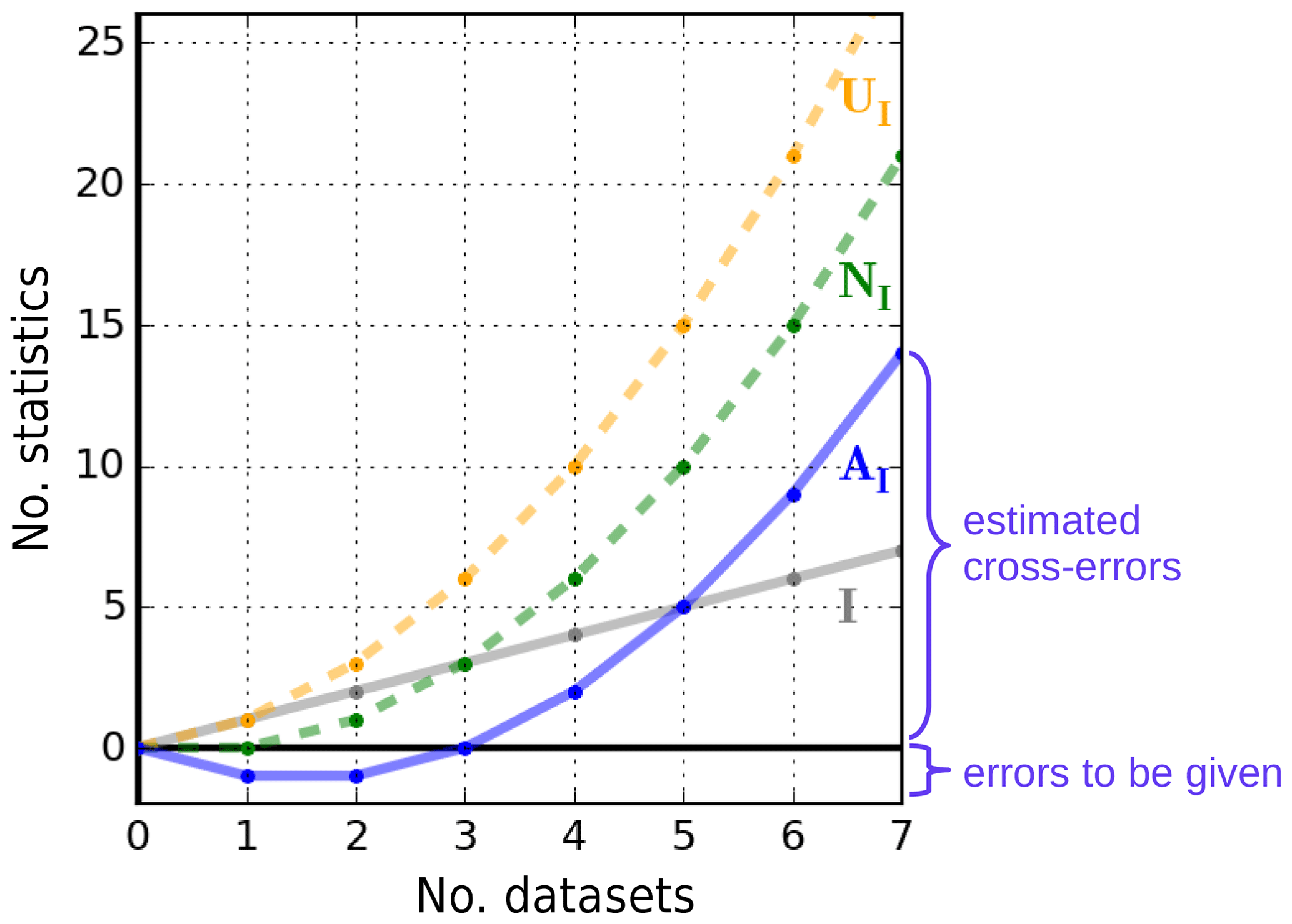
Figure 1 Relation between different numbers of statistics (covariances and cross-covariances) as a function of the number of datasets. Shown are I in solid gray (no. of datasets, no. of error covariances, and no. of required assumptions), U_I in dashed orange (no. of error statistics), N_I in dashed green (no. of residual covariances, no. of error dependencies, and no. of estimated error statistics), and A_I in solid blue (no. of estimated error cross-covariances).

Because N_I residual statistics are known, N_I of the U_I error statistics can be estimated, but the remaining I statistics have to be assumed in order to close the problem. The set of error statistics to be estimated can generally be chosen according to the specific application, but it will be shown that there are some constraints. Based on the mathematical theory provided in the following sections, Sect. 6.1 provides guidelines that ensure the solvability of the problem for a minimal number of assumptions.

In most applications of geophysical datasets, like in data assimilation, the estimation of error covariances is highly crucial, whereas their error cross-covariances are usually assumed to be negligible. Given the greater need to estimate the I error covariances, the remaining number of error cross-covariances that can be additionally estimated (A_I) is as follows:

$$\begin{array}{}\text{(3)}& A_I=N_I-I={\displaystyle \frac{\mathrm{1}}{\mathrm{2}}}\cdot I\cdot (I-\mathrm{3}).\end{array}$$

The relation between the number of datasets, residual covariances, and assumed and estimated error statistics is visualized in Fig. 1. The value for I=0 represents the mathematical extension of the problem, where no error nor residual statistics are required when no dataset is considered. For less than three datasets ($\mathrm{0}<I<\mathrm{3}$), A_I is negative, as the number of (known) residual covariances is smaller than the number of (unknown) error covariances (N_I<I); thus, the problem is underdetermined, even when all datasets are assumed to be independent (zero error cross-covariances). As in the case of data assimilation of two datasets (I=2), additional assumptions regarding error statistics are required. The same holds when only one dataset is available (I=1): the error covariance of this dataset remains unknown because no residual covariance can be formed. For three datasets (I=3), A_I is zero, meaning that the problem is fully determined under the assumption of independent errors (N_I=I, formulated in Sect. 4.1).

For more than three datasets (I>3), the number of (known) residual covariances exceeds the number of error covariances; this would lead to an overdetermined problem if independence among all datasets is assumed. Instead of solving an overdetermined problem, additional information can be used to calculate some error cross-covariances (formulated in Sect. 4.2). In other words, for I>3, not all datasets need to be assumed to be independent, and A_I gives the number of error cross-covariances that can be estimated in addition to the error covariances from all datasets. For example, half of the error cross-covariances can be estimated for I=5 $(\frac{A_{\mathrm{5}}}{N_{\mathrm{5}}}=\frac{\mathrm{5}}{\mathrm{10}})$, while two-thirds of them can be estimated for I=7 $(\frac{A_{\mathrm{7}}}{N_{\mathrm{7}}}=\frac{\mathrm{14}}{\mathrm{21}})$. Although the relative number of error cross-covariances that can be estimated increases with the number of datasets, an increasing number of $U_I-N_I=I$ assumptions – equal to the number of datasets – is required in order to close the problem because $U_I>N_I,\forall I>\mathrm{0}$.

Note that almost all numbers presented above apply to the general case, in which any combination of error covariances and cross-covariances may be given or assumed. While the interpretation of the numbers I, N_I, and U_I remains the same in all cases, the only difference is the interpretation of A_I, which is less meaningful when error covariances are also assumed.

3 Mathematical theory: exact formulation

This section gives the theoretical formulation for the exact statistical formulations of complete error covariance and cross-covariance matrices from fully spatiotemporally collocated datasets. Similar to the 3CH method, the errors are assumed to be random, independent among different realizations, but with common error statistics for each dataset. The notation is introduced in Sect. 3.1. While the true state and, thus, error statistics with respect to the truth are usually unknown, residual statistics can be calculated from residuals between each pair of datasets. At the same time, residual statistics contain information about the error statistics of the datasets involved. The expression of residual statistics as a function of error covariances and cross-covariances in Sect. 3.2 provides the basis for the subsequent mathematical theory. Based on these forward relations, inverse relations describe error statistics as a function of the residual statistics. The general equations of inverse relations are given in Sect. 3.3 and result in a highly underdetermined system of equations. Closed formulations of error statistics for three or more datasets under certain assumptions will be formulated in the following (Sect. 4).

This first part of the mathematical theory includes the following new elements: (i) the separation of cross-statistics into a symmetric error dependency and an error asymmetry (Sect. 3.1), (ii) the general formulation of residual statistics as a function of error statistics (Sect. 3.2.1 and 3.2.2), (iii) the demonstration of equivalence between residual covariances and cross-covariances (Sect. 3.2.3), and (iv) the general formulation of exact relations between residual- and error statistics (Sect. 3.3).

3.1 Notation

Suppose I datasets, each containing R realizations of spatiotemporally collocated state vectors ${\mathit{x}}_i,\forall i\in [\mathrm{1},I]$. Without loss of generality, the following formulation uses unbiased state vectors with a zero mean. In practice, each index i, j, k, and l may represent any geophysical dataset, like model forecasts, climatologies, in situ or remote-sensing observations, or other datasets.

Let ${\mathbf{\Gamma }}_{i;j;k;l}$ be the residual cross-covariance matrix between dataset residuals i−j and k−l with j≠i and l≠k, where each element (p,q) is given by the expectation over all realizations,

$$\begin{array}{}\text{(4)}& {\mathbf{\Gamma }}_{i;j;k;l}(p,q):=\stackrel{\mathrm{‾}}{\left[{\mathit{x}}_i\right(p)-{\mathit{x}}_j(p\left)\right]\left[{\mathit{x}}_k\right(q)-{\mathit{x}}_l(q\left)\right]},\end{array}$$

and the error cross-covariance matrix ${\mathbf{X}}_{\stackrel{\mathrm{̃}}{i};\stackrel{\mathrm{̃}}{j}}$ between the errors of two datasets i and j with respect to the true state x_T,

$$\begin{array}{}\text{(5)}& {\mathbf{X}}_{\stackrel{\mathrm{̃}}{i};\stackrel{\mathrm{̃}}{j}}(p,q):=\stackrel{\mathrm{‾}}{\left[{\mathit{x}}_i\right(p)-{\mathit{x}}_T(p\left)\right]\left[{\mathit{x}}_j\right(q)-{\mathit{x}}_T(q\left)\right]}.\end{array}$$

Here, the tilde above a dataset index indicates its deviation from the truth and the overbar denotes the expectation over all R realizations. Note that x_i(p) is a scalar element of the dataset vector.

In the symmetric case, each element (p,q) of the residual covariance matrix of i−j with j≠i, is given by

$$\begin{array}{}\text{(6)}& \begin{array}{rl}{\mathbf{\Gamma }}_{i;j}(p,q)& :={\mathbf{\Gamma }}_{i;j;i;j}(p,q)\\ & \stackrel{\left(\mathrm{4}\right)}{=}\stackrel{\mathrm{‾}}{\left[{\mathit{x}}_i\right(p)-{\mathit{x}}_j(p\left)\right]\left[{\mathit{x}}_i\right(q)-{\mathit{x}}_j(q\left)\right]}\end{array}\end{array}$$

and the error covariance matrix ${\mathbf{C}}_{\stackrel{\mathrm{̃}}{i}}$ of a dataset i with respect to the true state x_T

$$\begin{array}{}\text{(7)}& \begin{array}{rl}{\mathbf{C}}_{\stackrel{\mathrm{̃}}{i}}(p,q)& :={\mathbf{X}}_{\stackrel{\mathrm{̃}}{i};\stackrel{\mathrm{̃}}{i}}(p,q)\\ & \stackrel{\left(\mathrm{5}\right)}{=}\stackrel{\mathrm{‾}}{\left[{\mathit{x}}_i\right(p)-{\mathit{x}}_T(p\left)\right]\left[{\mathit{x}}_i\right(q)-{\mathit{x}}_T(q\left)\right]}.\end{array}\end{array}$$

Here, the numbers in parentheses above an equal sign indicate other equations that were used to retrieve the right-hand side.

Note that residual and error cross-covariance matrices are generally asymmetric in the non-scalar formulation presented here, but the following relations hold for residual as well as (similarly) for error cross-covariance matrices:

$$\begin{array}{}\text{(8)}& {\displaystyle }{\mathbf{\Gamma }}_{i;j;k;l}\stackrel{\left(\mathrm{4}\right)}{=}-{\mathbf{\Gamma }}_{j;i;k;l}\stackrel{\left(\mathrm{4}\right)}{=}& {\displaystyle }-{\mathbf{\Gamma }}_{i;j;l;k}\stackrel{\left(\mathrm{4}\right)}{=}{\mathbf{\Gamma }}_{j;i;l;k}\text{(9)}& {\displaystyle }{\mathbf{\Gamma }}_{i;j;k;l}\stackrel{\left(\mathrm{4}\right)}{=}& {\displaystyle }[{\mathbf{\Gamma }}_{k;l;i;j}{]}^{\mathrm{T}}\text{(10)}& {\displaystyle }{\mathbf{X}}_{\stackrel{\mathrm{̃}}{i};\stackrel{\mathrm{̃}}{j}}\stackrel{\left(\mathrm{5}\right)}{=}& {\displaystyle }[{\mathbf{X}}_{\stackrel{\mathrm{̃}}{j};\stackrel{\mathrm{̃}}{i}}{]}^{\mathrm{T}}.\end{array}$$

The symmetric properties of residual and error covariances follow directly from their definition:

$$\begin{array}{}\text{(11)}& {\displaystyle }{\mathbf{\Gamma }}_{i;j}\stackrel{\left(\mathrm{6}\right)}{=}& {\displaystyle }{\mathbf{\Gamma }}_{j;i}\text{(12)}& {\displaystyle }[{\mathbf{\Gamma }}_{i;j}{]}^{\mathrm{T}}\stackrel{\left(\mathrm{6}\right)}{=}& {\displaystyle }{\mathbf{\Gamma }}_{i;j}.\end{array}$$

The sum of an (asymmetric) cross-covariance matrix and its transpose is denoted as dependency. For example, the sum of error cross-covariance matrices between i and j is denoted as the error dependency matrix ${\mathbf{D}}_{\stackrel{\mathrm{̃}}{i};\stackrel{\mathrm{̃}}{j}}$:

$$\begin{array}{}\text{(13)}& {\mathbf{D}}_{\stackrel{\mathrm{̃}}{i};\stackrel{\mathrm{̃}}{j}}:={\mathbf{X}}_{\stackrel{\mathrm{̃}}{i};\stackrel{\mathrm{̃}}{j}}+{\mathbf{X}}_{\stackrel{\mathrm{̃}}{j};\stackrel{\mathrm{̃}}{i}}.\end{array}$$

Although error cross-covariances may be asymmetric, the error dependency matrix is symmetric by definition:

$$\begin{array}{}\text{(14)}& {\displaystyle }{\mathbf{D}}_{\stackrel{\mathrm{̃}}{i};\stackrel{\mathrm{̃}}{j}}\stackrel{\left(\mathrm{13}\right)}{=}{\mathbf{X}}_{\stackrel{\mathrm{̃}}{i};\stackrel{\mathrm{̃}}{j}}+{\mathbf{X}}_{\stackrel{\mathrm{̃}}{j};\stackrel{\mathrm{̃}}{i}}\stackrel{\left(\mathrm{13}\right)}{=}{\mathbf{D}}_{\stackrel{\mathrm{̃}}{j};\stackrel{\mathrm{̃}}{i}},\text{(15)}& {\displaystyle }{\mathbf{D}}_{\stackrel{\mathrm{̃}}{i};\stackrel{\mathrm{̃}}{j}}\stackrel{\left(\mathrm{13}\right)}{=}{\mathbf{X}}_{\stackrel{\mathrm{̃}}{i};\stackrel{\mathrm{̃}}{j}}+{\mathbf{X}}_{\stackrel{\mathrm{̃}}{j};\stackrel{\mathrm{̃}}{i}}\stackrel{\left(\mathrm{10}\right)}{=}[{\mathbf{X}}_{\stackrel{\mathrm{̃}}{j};\stackrel{\mathrm{̃}}{i}}{]}^{\mathrm{T}}+[{\mathbf{X}}_{\stackrel{\mathrm{̃}}{i};\stackrel{\mathrm{̃}}{j}}{]}^{\mathrm{T}}\stackrel{\left(\mathrm{13}\right)}{=}[{\mathbf{D}}_{\stackrel{\mathrm{̃}}{i};\stackrel{\mathrm{̃}}{j}}{]}^{\mathrm{T}}.\end{array}$$

Likewise, the sum of the residual cross-covariance matrices between i−j and k−l with j≠i and l≠k is denoted as the residual dependency matrix ${\mathbf{D}}_{i;j;k;l}$:

$$\begin{array}{}\text{(16)}& {\mathbf{D}}_{i;j;k;l}:={\mathbf{\Gamma }}_{i;j;k;l}+{\mathbf{\Gamma }}_{k;l;i;j}.\end{array}$$

The difference between a cross-covariance matrix and its transpose is a measure of asymmetry in the cross-covariances and is, therefore, denoted as asymmetry. For example, the difference between the error cross-covariance matrices between i and j is denoted as the error asymmetry matrix ${\mathbf{Y}}_{\stackrel{\mathrm{̃}}{i};\stackrel{\mathrm{̃}}{j}}$:

$$\begin{array}{}\text{(17)}& {\mathbf{Y}}_{\stackrel{\mathrm{̃}}{i};\stackrel{\mathrm{̃}}{j}}:={\mathbf{X}}_{\stackrel{\mathrm{̃}}{i};\stackrel{\mathrm{̃}}{j}}-{\mathbf{X}}_{\stackrel{\mathrm{̃}}{j};\stackrel{\mathrm{̃}}{i}}.\end{array}$$

Likewise, the difference between the residual cross-covariance matrices between i−j and k−l with j≠i and l≠k is denoted as the residual asymmetry matrix ${\mathbf{Y}}_{i;j;k;l}$:

$$\begin{array}{}\text{(18)}& {\mathbf{Y}}_{i;j;k;l}:={\mathbf{\Gamma }}_{i;j;k;l}-{\mathbf{\Gamma }}_{k;l;i;j}.\end{array}$$

3.2 Residual statistics

For real geophysical problems, the available statistical information comprises (i) the residual covariance matrices of each pair of datasets and (ii) the residual cross-covariance matrices between different residuals of datasets. The forward relations of residual covariances and residual cross-covariances as functions of error statistics are formulated in the following. For the estimation of error statistics, it is important to quantify the number of independent input statistics that determines the number of possible error estimations. Therefore, this section also includes an evaluation of the relation between residual cross-covariances and residual covariances in order to specify the additional information content of residual cross-covariances.

3.2.1 Residual covariances

Each element (p,q) of the residual covariance matrix between two input datasets i and j can be written as a function of their error statistics as follows:

$$\begin{array}{c}{\displaystyle }{\mathbf{\Gamma }}_{i;j}(p,q)\stackrel{\left(\mathrm{6}\right)}{=}\stackrel{\mathrm{‾}}{\begin{array}{c}\mathit{\left\{}\right[{\mathit{x}}_i\left(p\right)-{\mathit{x}}_T\left(p\right)]-[{\mathit{x}}_j\left(p\right)-{\mathit{x}}_T\left(p\right)\left]\mathit{\right\}}\\ \stackrel{\mathrm{‾}}{\cdot \mathit{\left\{}\right[{\mathit{x}}_i\left(q\right)-{\mathit{x}}_T\left(q\right)]-[{\mathit{x}}_j\left(q\right)-{\mathit{x}}_T\left(q\right)\left]\mathit{\right\}}}\end{array}}\\ \text{(19)}& {\displaystyle }\begin{array}{rl}& \stackrel{\left(\mathrm{5}\right),\left(\mathrm{7}\right)}{=}{\mathbf{C}}_{\stackrel{\mathrm{̃}}{i}}(p,q)-{\mathbf{X}}_{\stackrel{\mathrm{̃}}{i};\stackrel{\mathrm{̃}}{j}}(p,q)-{\mathbf{X}}_{\stackrel{\mathrm{̃}}{j};\stackrel{\mathrm{̃}}{i}}(p,q)\\ & +{\mathbf{C}}_{\stackrel{\mathrm{̃}}{j}}(p,q).\end{array}\end{array}$$

Thus, the complete residual covariance matrix of i−j is expressed as follows:

$$\begin{array}{}\text{(20)}& {\mathbf{\Gamma }}_{i;j}\stackrel{\left(\mathrm{19}\right)}{=}\underset{\text{“independent residual”}}{\underbrace{{\mathbf{C}}_{\stackrel{\mathrm{̃}}{i}}+{\mathbf{C}}_{\stackrel{\mathrm{̃}}{j}}}}-\underset{\text{“error dependency”}=:{\mathbf{D}}_{\stackrel{\mathrm{̃}}{i};\stackrel{\mathrm{̃}}{j}}.}{\underbrace{[{\mathbf{X}}_{\stackrel{\mathrm{̃}}{i};\stackrel{\mathrm{̃}}{j}}+{\mathbf{X}}_{\stackrel{\mathrm{̃}}{j};\stackrel{\mathrm{̃}}{i}}]}}\end{array}$$

Equation (20) is an exact formulation of the complete residual covariance matrix of any pair of datasets i−j. It holds for all combinations of datasets without any further assumption like independent errors. Thus, the residual covariance of any dataset pair consists of (i) the independent residual associated with sum of the error covariances of each dataset minus (ii) the error dependency corresponding to the sum of their error cross-covariances.

Note that, although the error dependency matrix is symmetric by definition, it is the sum of two error cross-covariances that are generally asymmetric and, thus, differ in the non-scalar formulation. In the scalar case, the two error cross-covariances reduce to their common error cross-variance and the residual covariance reduces to the scalar formulation of the variance, as shown in studies such as Anthes and Rieckh (2018) and Sjoberg et al. (2021).

3.2.2 Residual cross-covariances

Each element (p,q) of the residual cross-covariance matrix between two input datasets i−j and k−l can be written as a function of their error cross-covariances,

$$\begin{array}{c}{\displaystyle }{\mathbf{\Gamma }}_{i;j;k;l}(p,q)\stackrel{\left(\mathrm{4}\right)}{=}\stackrel{\mathrm{‾}}{\begin{array}{c}\mathit{\left\{}\right[{\mathit{x}}_i\left(p\right)-{\mathit{x}}_T\left(p\right)]-[{\mathit{x}}_j\left(p\right)-{\mathit{x}}_T\left(p\right)\left]\mathit{\right\}}\\ \stackrel{\mathrm{‾}}{\cdot \mathit{\left\{}\right[{\mathit{x}}_k\left(q\right)-{\mathit{x}}_T\left(q\right)]-[{\mathit{x}}_l\left(q\right)-{\mathit{x}}_T\left(q\right)\left]\mathit{\right\}}}\end{array}}\\ \text{(21)}& {\displaystyle }\begin{array}{rl}& \stackrel{\left(\mathrm{5}\right)}{=}{\mathbf{X}}_{\stackrel{\mathrm{̃}}{i};\stackrel{\mathrm{̃}}{k}}(p,q)-{\mathbf{X}}_{\stackrel{\mathrm{̃}}{i};\stackrel{\mathrm{̃}}{l}}(p,q)-{\mathbf{X}}_{\stackrel{\mathrm{̃}}{j};\stackrel{\mathrm{̃}}{k}}(p,q)\\ & +{\mathbf{X}}_{\stackrel{\mathrm{̃}}{j};\stackrel{\mathrm{̃}}{l}}(p,q),\end{array}\end{array}$$

and, thus, the complete residual cross-covariance matrix between i−j and k−l,

$$\begin{array}{}\text{(22)}& {\mathbf{\Gamma }}_{i;j;k;l}\stackrel{\left(\mathrm{21}\right)}{=}{\mathbf{X}}_{\stackrel{\mathrm{̃}}{i};\stackrel{\mathrm{̃}}{k}}-{\mathbf{X}}_{\stackrel{\mathrm{̃}}{i};\stackrel{\mathrm{̃}}{l}}-{\mathbf{X}}_{\stackrel{\mathrm{̃}}{j};\stackrel{\mathrm{̃}}{k}}+{\mathbf{X}}_{\stackrel{\mathrm{̃}}{j};\stackrel{\mathrm{̃}}{l}}.\end{array}$$

Equation (22) is a generalized form of Eq. (20) with residuals between different datasets (i−j; k−l). It consists of four error cross-covariances of the datasets involved. This formulation of residual statistics as a function of error statistics provides the basis for the complete theoretical derivation of error estimates in this study. In contrast to the symmetric residual covariance matrix, the residual cross-covariance matrix may be asymmetric for asymmetric error cross-covariances.

3.2.3 Relation of residual statistics

In the following, it is demonstrated that combinations of residual cross-covariances contain the same statistical information as residual covariance matrices.

For k=i, the residual dependency between i−j and i−l can be expressed as combination of three residual covariances:

$$\begin{array}{}\text{(23)}& \begin{array}{rl}{\mathbf{\Gamma }}_{i;l}+{\mathbf{\Gamma }}_{j;i}-{\mathbf{\Gamma }}_{j;l}\stackrel{\left(\mathrm{6}\right)}{=}& \stackrel{\mathrm{‾}}{\left[{\mathit{x}}_i\right(p)-{\mathit{x}}_l(p\left)\right]\left[{\mathit{x}}_i\right(q)-{\mathit{x}}_l(q\left)\right]}\\ & +\stackrel{\mathrm{‾}}{\left[{\mathit{x}}_j\right(p)-{\mathit{x}}_i(p\left)\right]\left[{\mathit{x}}_j\right(q)-{\mathit{x}}_i(q\left)\right]}\\ & -\stackrel{\mathrm{‾}}{\left[{\mathit{x}}_j\right(p)-{\mathit{x}}_l(p\left)\right]\left[{\mathit{x}}_j\right(q)-{\mathit{x}}_l(q\left)\right]}\\ =& \stackrel{\mathrm{‾}}{\left[{\mathit{x}}_i\right(p\left)\right]\left[{\mathit{x}}_i\right(q\left)\right]}-\stackrel{\mathrm{‾}}{\left[{\mathit{x}}_i\right(p\left)\right]\left[{\mathit{x}}_l\right(q\left)\right]}\\ & -\stackrel{\mathrm{‾}}{\left[{\mathit{x}}_l\right(p\left)\right]\left[{\mathit{x}}_i\right(q\left)\right]}\cancel{+\stackrel{\mathrm{‾}}{\left[{\mathit{x}}_l\right(p\left)\right]\left[{\mathit{x}}_l\right(q\left)\right]}}\\ & \cancel{+\stackrel{\mathrm{‾}}{\left[{\mathit{x}}_j\right(p\left)\right]\left[{\mathit{x}}_j\right(q\left)\right]}}-\stackrel{\mathrm{‾}}{\left[{\mathit{x}}_j\right(p\left)\right]\left[{\mathit{x}}_i\right(q\left)\right]}\\ & -\stackrel{\mathrm{‾}}{\left[{\mathit{x}}_i\right(p\left)\right]\left[{\mathit{x}}_j\right(q\left)\right]}+\stackrel{\mathrm{‾}}{\left[{\mathit{x}}_i\right(p\left)\right]\left[{\mathit{x}}_i\right(q\left)\right]}\\ & \cancel{-\stackrel{\mathrm{‾}}{\left[{\mathit{x}}_j\right(p\left)\right]\left[{\mathit{x}}_j\right(q\left)\right]}}+\stackrel{\mathrm{‾}}{\left[{\mathit{x}}_j\right(p\left)\right]\left[{\mathit{x}}_l\right(q\left)\right]}\\ & +\stackrel{\mathrm{‾}}{\left[{\mathit{x}}_l\right(p\left)\right]\left[{\mathit{x}}_j\right(q\left)\right]}\cancel{-\stackrel{\mathrm{‾}}{\left[{\mathit{x}}_l\right(p\left)\right]\left[{\mathit{x}}_l\right(q\left)\right]}}\\ =& \stackrel{\mathrm{‾}}{\left[{\mathit{x}}_i\right(p)-{\mathit{x}}_j(p\left)\right]\left[{\mathit{x}}_i\right(q)-{\mathit{x}}_l(q\left)\right]}\\ & +\stackrel{\mathrm{‾}}{\left[{\mathit{x}}_i\right(p)-{\mathit{x}}_l(p\left)\right]\left[{\mathit{x}}_i\right(q)-{\mathit{x}}_j(q\left)\right]}\\ \stackrel{\left(\mathrm{4}\right)}{=}& {\mathbf{\Gamma }}_{i;j;i;l}+{\mathbf{\Gamma }}_{i;l;i;j}.\end{array}\end{array}$$

The relation between residual covariances and residual cross-covariances in Eq. (23) is exact and holds for all datasets without any further assumptions. In the case of symmetric residual cross-covariances $({\mathbf{\Gamma }}_{i;j;i;l}={\mathbf{\Gamma }}_{i;l;i;j}\stackrel{\left(\mathrm{23}\right)}{=}\frac{\mathrm{1}}{\mathrm{2}}[{\mathbf{\Gamma }}_{i;l}+{\mathbf{\Gamma }}_{j;i}-{\mathbf{\Gamma }}_{j;l}\left]\right)$, the residual cross-covariance matrices are fully determined by the symmetric residual covariances.

In the general asymmetric case, Eq. (23) can be rewritten as follows:

$$\begin{array}{}\text{(24)}& \begin{array}{rl}{\mathbf{\Gamma }}_{i;l}+{\mathbf{\Gamma }}_{j;i}-{\mathbf{\Gamma }}_{j;l}& \stackrel{\left(\mathrm{23}\right)}{=}{\mathbf{\Gamma }}_{i;j;i;l}+{\mathbf{\Gamma }}_{i;l;i;j}\\ & \stackrel{\left(\mathrm{18}\right)}{=}{\mathbf{\Gamma }}_{i;j;i;l}+[{\mathbf{\Gamma }}_{i;j;i;l}-{\mathbf{Y}}_{i;j;i;l}]\\ ⟺{\mathbf{\Gamma }}_{i;j;i;l}& ={\displaystyle \frac{\mathrm{1}}{\mathrm{2}}}[{\mathbf{\Gamma }}_{i;l}+{\mathbf{\Gamma }}_{j;i}-{\mathbf{\Gamma }}_{j;l}]+{\displaystyle \frac{\mathrm{1}}{\mathrm{2}}}{\mathbf{Y}}_{i;j;i;l}.\end{array}\end{array}$$

Equation (24) shows that each individual residual cross-covariance consists of a symmetric contribution including residual covariances between the datasets and an asymmetric contribution that is half of the related residual asymmetry matrix. Thus, residual cross-covariances may only provide additional information on asymmetries of error statistics, not on symmetric statistics (like error covariances).

3.3 Exact error statistics

As an extension to previous work, this section provides generalized formulations of error covariances, cross-covariances, and dependencies in matrix form. These formulations are based on the relations between residual and error statistics in Eqs. (20) and (22). Note that the general formulations presented here do not provide a closed system of equations that can be solved in real applications. They serve as a basis for the approximate solutions that are formulated in the subsequent section.

3.3.1 Error statistics from residual covariances

Equation (20) shows that each residual covariance matrix can be expressed by the error covariances of the two datasets involved and their error dependency. The goal is to find an inverse formulation of an error covariance matrix as a function of the residual covariances that does not include other (unknown) error covariances matrices. By combining the formulations of three residuals Γ_i;j, Γ_j;k, and Γ_k;i between the same three datasets i, j, and k and expressing each using Eq. (20), a single error covariance can be eliminated:

$$\begin{array}{ll}\text{(25)}& {\displaystyle }{\mathbf{C}}_{\stackrel{\mathrm{̃}}{i}}\stackrel{(\mathrm{20}{)}_{ij}}{=}& {\displaystyle }{\mathbf{\Gamma }}_{i;j}+{\mathbf{D}}_{\stackrel{\mathrm{̃}}{i};\stackrel{\mathrm{̃}}{j}}-{\mathbf{C}}_{\stackrel{\mathrm{̃}}{j}}{\displaystyle }\stackrel{(\mathrm{20}{)}_{jk}}{=}& {\displaystyle }{\mathbf{\Gamma }}_{i;j}+{\mathbf{D}}_{\stackrel{\mathrm{̃}}{i};\stackrel{\mathrm{̃}}{j}}-{\mathbf{\Gamma }}_{j;k}-{\mathbf{D}}_{\stackrel{\mathrm{̃}}{j};\stackrel{\mathrm{̃}}{k}}+{\mathbf{C}}_{\stackrel{\mathrm{̃}}{k}}\\ {\displaystyle }\stackrel{(\mathrm{20}{)}_{ki}}{=}& {\displaystyle }{\mathbf{\Gamma }}_{i;j}+{\mathbf{D}}_{\stackrel{\mathrm{̃}}{i};\stackrel{\mathrm{̃}}{j}}-{\mathbf{\Gamma }}_{j;k}-{\mathbf{D}}_{\stackrel{\mathrm{̃}}{j};\stackrel{\mathrm{̃}}{k}}\\ \text{(26)}& {\displaystyle }& {\displaystyle }+{\mathbf{\Gamma }}_{k;i}+{\mathbf{D}}_{\stackrel{\mathrm{̃}}{k};\stackrel{\mathrm{̃}}{i}}-{\mathbf{C}}_{\stackrel{\mathrm{̃}}{i}}\end{array}$$

$$\begin{array}{}\text{(27)}& ⟺{\mathbf{C}}_{\stackrel{\mathrm{̃}}{i}}={\displaystyle \frac{\mathrm{1}}{\mathrm{2}}}[\underset{\text{“independent contribution”}}{\underbrace{{\mathbf{\Gamma }}_{i;j}+{\mathbf{\Gamma }}_{k;i}-{\mathbf{\Gamma }}_{j;k}}}+\underset{\text{“dependent contribution”}}{\underbrace{{\mathbf{D}}_{\stackrel{\mathrm{̃}}{i};\stackrel{\mathrm{̃}}{j}}+{\mathbf{D}}_{\stackrel{\mathrm{̃}}{k};\stackrel{\mathrm{̃}}{i}}-{\mathbf{D}}_{\stackrel{\mathrm{̃}}{j};\stackrel{\mathrm{̃}}{k}}}}],\end{array}$$

where the indication of the equations used, which is given above the equal signs, is extended by indices that denote the datasets to which this equation has been applied. For example, “$\stackrel{(\mathrm{20}{)}_{ki}}{=}$” indicates that the relation in Eq. (20) was applied to datasets k and i to achieve the right-hand side.

Equation (27) provides a general formulation of error covariances as a function of residual covariances and error dependencies. It holds for all combinations of datasets without any further assumptions (e.g., independence). Thus, each error covariance can be formulated as a sum of an independent contribution of three residual covariances with respect to any pair of other datasets and a dependent contribution of the three related error dependencies. While the independent contribution can be calculated from residual statistics between input datasets, the dependent contribution is generally unknown in real applications.

Given I datasets, the total number of different formulations of each error covariance in Eq. (27) is determined by the number of different pairs of the other datasets, which is ${\sum }_{i=\mathrm{1}}^{I-\mathrm{2}}i=\frac{\mathrm{1}}{\mathrm{2}}(I-\mathrm{1})(I-\mathrm{2})$ (see also Sjoberg et al., 2021). The scalar equivalent of Eq. (27) where the dependency matrices reduce to twice the error cross-variances has been previously formulated in the 3CH method in studies such as Anthes and Rieckh (2018) and Sjoberg et al. (2021). Very recently, the full matrix form was used by Nielsen et al. (2022) and Todling et al. (2022). Note that, in the literature, the dependent contribution in Eq. (27) is denoted as cross-covariances between the errors.

Equation (26) can be generalized by replacing the closed series of the three dataset pairs (i;j), (j;k), and (k;i) with a closed series of F dataset pairs, $(i_{\mathrm{1}};i_{\mathrm{2}}),(i_{\mathrm{2}};i_{\mathrm{3}})$, …, $(i_{F-\mathrm{1}};i_F),(i_F;i_{\mathrm{1}})$, for any $\mathrm{3}\le F\le I$ (where I is the number of datasets):

$$\begin{array}{}\text{(28)}& \begin{array}{rl}{\mathbf{C}}_{\stackrel{\mathrm{̃}}{i_{\mathrm{1}}}}\stackrel{\left(\mathrm{20}\right)}{=}& \sum _{f=\mathrm{1}}^{F-\mathrm{1}}(-\mathrm{1}{)}^{f-\mathrm{1}}\left[{\mathbf{\Gamma }}_{i_f;i_{f+\mathrm{1}}}+{\mathbf{D}}_{\stackrel{\mathrm{̃}}{i_f};\stackrel{\mathrm{̃}}{i_{f+\mathrm{1}}}}\right]\\ & +(-\mathrm{1}{)}^{F-\mathrm{1}}\left[{\mathbf{\Gamma }}_{i_F;i_{\mathrm{1}}}+{\mathbf{D}}_{\stackrel{\mathrm{̃}}{i_F};\stackrel{\mathrm{̃}}{i_{\mathrm{1}}}}\right]+(-\mathrm{1}{)}^F{\mathbf{C}}_{\stackrel{\mathrm{̃}}{i_{\mathrm{1}}}}.\end{array}\end{array}$$

Because of changing signs, Eq. (28) can only be solved for the error covariance ${\mathbf{C}}_{\stackrel{\mathrm{̃}}{i_{\mathrm{1}}}}$ if F is odd. If F is even, ${\mathbf{C}}_{\stackrel{\mathrm{̃}}{i_{\mathrm{1}}}}$ cancels out, cannot be eliminated, and Eq. (28) could be solved for one error dependency instead. If F is odd, the generalized formulation for ${\mathbf{C}}_{\stackrel{\mathrm{̃}}{i_{\mathrm{1}}}}$ becomes the following:

$$\begin{array}{}\text{(29)}& \begin{array}{rl}{\mathbf{C}}_{\stackrel{\mathrm{̃}}{i_{\mathrm{1}}}}\stackrel{\left(\mathrm{28}\right)}{=}& {\displaystyle \frac{\mathrm{1}}{\mathrm{2}}}[\underset{\text{“independent contribution”}}{\underbrace{\left(\sum _{f=\mathrm{1}}^{F-\mathrm{1}}\right(-\mathrm{1}{)}^{f-\mathrm{1}}{\mathbf{\Gamma }}_{i_f;i_{f+\mathrm{1}}})+{\mathbf{\Gamma }}_{i_F;i_{\mathrm{1}}}}}\\ & +\underset{\text{“dependent contribution”}}{\underbrace{\left(\sum _{f=\mathrm{1}}^{F-\mathrm{1}}\right(-\mathrm{1}{)}^{f-\mathrm{1}}{\mathbf{D}}_{\stackrel{\mathrm{̃}}{i_f};\stackrel{\mathrm{̃}}{i_{f+\mathrm{1}}}})+{\mathbf{D}}_{\stackrel{\mathrm{̃}}{i_F};\stackrel{\mathrm{̃}}{i_{\mathrm{1}}}}}}],\\ & \forall F\text{ odd }\wedge \mathrm{3}\le F\le I,\end{array}\end{array}$$

where Eq. (27) results from setting F=3 with indices i₁=i, i₂=j, and i₃=k. Note that, in any case, the number of assumed and estimated error statistics remains consistent with the general framework in Sect. 2.

A formulation of each individual error dependency matrix as a function of the error covariances of the two datasets and their residual covariance results directly from Eq. (20):

$$\begin{array}{}\text{(30)}& {\mathbf{D}}_{\stackrel{\mathrm{̃}}{i};\stackrel{\mathrm{̃}}{j}}\stackrel{\left(\mathrm{20}\right)}{=}{\mathbf{C}}_{\stackrel{\mathrm{̃}}{i}}+{\mathbf{C}}_{\stackrel{\mathrm{̃}}{j}}-{\mathbf{\Gamma }}_{i;j}.\end{array}$$

Being a symmetric matrix, residual covariances cannot provide information on error asymmetries nor on the asymmetric components of error cross-covariances. Only the symmetric component of error cross-covariances could be estimated from half the error dependency, which is equivalent to a zero error asymmetry matrix:

$$\begin{array}{}\text{(31)}& \begin{array}{rl}& {\mathbf{D}}_{\stackrel{\mathrm{̃}}{i};\stackrel{\mathrm{̃}}{j}}+{\mathbf{Y}}_{\stackrel{\mathrm{̃}}{i};\stackrel{\mathrm{̃}}{j}}\stackrel{\left(\mathrm{13}\right),\left(\mathrm{17}\right)}{=}\left[{\mathbf{X}}_{\stackrel{\mathrm{̃}}{i};\stackrel{\mathrm{̃}}{j}}\cancel{+{\mathbf{X}}_{\stackrel{\mathrm{̃}}{j};\stackrel{\mathrm{̃}}{i}}}\right]+\left[{\mathbf{X}}_{\stackrel{\mathrm{̃}}{i};\stackrel{\mathrm{̃}}{j}}\cancel{-{\mathbf{X}}_{\stackrel{\mathrm{̃}}{j};\stackrel{\mathrm{̃}}{i}}}\right]\\ & ⟺{\mathbf{X}}_{\stackrel{\mathrm{̃}}{i};\stackrel{\mathrm{̃}}{j}}={\displaystyle \frac{\mathrm{1}}{\mathrm{2}}}[{\mathbf{D}}_{\stackrel{\mathrm{̃}}{i};\stackrel{\mathrm{̃}}{j}}+{\mathbf{Y}}_{\stackrel{\mathrm{̃}}{i};\stackrel{\mathrm{̃}}{j}}].\end{array}\end{array}$$

3.3.2 Error statistics from residual cross-covariances

The general forward formulation of residual cross-covariances in Eq. (22) consists of error cross-covariances of the four datasets involved. Setting, for example, k=i provides an inverse formulation of error covariances of i:

$$\begin{array}{}\text{(32)}& \begin{array}{rl}& {\mathbf{\Gamma }}_{i;j;i;l}\stackrel{\left(\mathrm{22}\right)}{=}{\mathbf{C}}_{\stackrel{\mathrm{̃}}{i}}-{\mathbf{X}}_{\stackrel{\mathrm{̃}}{i};\stackrel{\mathrm{̃}}{l}}-{\mathbf{X}}_{\stackrel{\mathrm{̃}}{j};\stackrel{\mathrm{̃}}{i}}+{\mathbf{X}}_{\stackrel{\mathrm{̃}}{j};\stackrel{\mathrm{̃}}{l}}\\ & ⟺{\mathbf{C}}_{\stackrel{\mathrm{̃}}{i}}={\mathbf{\Gamma }}_{i;j;i;l}+{\mathbf{X}}_{\stackrel{\mathrm{̃}}{i};\stackrel{\mathrm{̃}}{l}}+{\mathbf{X}}_{\stackrel{\mathrm{̃}}{j};\stackrel{\mathrm{̃}}{i}}-{\mathbf{X}}_{\stackrel{\mathrm{̃}}{j};\stackrel{\mathrm{̃}}{l}}.\end{array}\end{array}$$

The scalar formulation of Eq. (32) was previously given in Zwieback et al. (2012).

Similarly to Eq. (27) from residual covariances, the number of formulations of each error covariance from different pairs of other datasets in Eq. (32) is ${\sum }_{i=\mathrm{1}}^{I-\mathrm{2}}i=\frac{\mathrm{1}}{\mathrm{2}}(I-\mathrm{1})(I-\mathrm{2})$. In addition, there are four possibilities to write each error covariance from the same pairs of other datasets using the relations of residual cross-covariances in Eq. (8). Each of the four possibilities results from setting both indices of one pair of datasets in the definition of the residual cross-covariances in Eq. (22) to the same value.

Two of the error cross-covariances in Eq. (32) can be rewritten by applying Eq. (32) to the error covariance of dataset j:

$$\begin{array}{}\text{(33)}& \begin{array}{rl}& {\mathbf{C}}_{\stackrel{\mathrm{̃}}{j}}\stackrel{(\mathrm{32}{)}_j}{=}{\mathbf{\Gamma }}_{j;i;j;l}+{\mathbf{X}}_{\stackrel{\mathrm{̃}}{j};\stackrel{\mathrm{̃}}{l}}+{\mathbf{X}}_{\stackrel{\mathrm{̃}}{i};\stackrel{\mathrm{̃}}{j}}-{\mathbf{X}}_{\stackrel{\mathrm{̃}}{i};\stackrel{\mathrm{̃}}{l}}\\ & ⟺{\mathbf{X}}_{\stackrel{\mathrm{̃}}{i};\stackrel{\mathrm{̃}}{l}}-{\mathbf{X}}_{\stackrel{\mathrm{̃}}{j};\stackrel{\mathrm{̃}}{l}}={\mathbf{\Gamma }}_{j;i;j;l}+{\mathbf{X}}_{\stackrel{\mathrm{̃}}{i};\stackrel{\mathrm{̃}}{j}}-{\mathbf{C}}_{\stackrel{\mathrm{̃}}{j}}.\end{array}\end{array}$$

With this, Eq. (32) becomes the following:

$$\begin{array}{}\text{(34)}& \begin{array}{rl}{\mathbf{C}}_{\stackrel{\mathrm{̃}}{i}}\stackrel{\left(\mathrm{33}\right)}{=}& {\mathbf{\Gamma }}_{i;j;i;l}+{\mathbf{\Gamma }}_{j;i;j;l}-{\mathbf{C}}_{\stackrel{\mathrm{̃}}{j}}+{\mathbf{X}}_{\stackrel{\mathrm{̃}}{i};\stackrel{\mathrm{̃}}{j}}+{\mathbf{X}}_{\stackrel{\mathrm{̃}}{j};\stackrel{\mathrm{̃}}{i}}\\ \stackrel{\left(\mathrm{13}\right)}{=}& {\mathbf{\Gamma }}_{i;j;i;l}+{\mathbf{\Gamma }}_{j;i;j;l}-{\mathbf{C}}_{\stackrel{\mathrm{̃}}{j}}+{\mathbf{D}}_{\stackrel{\mathrm{̃}}{i};\stackrel{\mathrm{̃}}{j}}.\end{array}\end{array}$$

Because the residual cross-covariances can be rewritten as

$$\begin{array}{}\text{(35)}& \begin{array}{rl}{\mathbf{\Gamma }}_{i;j;i;l}+{\mathbf{\Gamma }}_{j;i;j;l}& \stackrel{\left(\mathrm{32}\right),\left(\mathrm{33}\right)}{=}{\mathbf{C}}_{\stackrel{\mathrm{̃}}{i}}\cancel{-{\mathbf{X}}_{\stackrel{\mathrm{̃}}{i};\stackrel{\mathrm{̃}}{l}}}-{\mathbf{X}}_{\stackrel{\mathrm{̃}}{j};\stackrel{\mathrm{̃}}{i}}\cancel{+{\mathbf{X}}_{\stackrel{\mathrm{̃}}{j};\stackrel{\mathrm{̃}}{l}}}\\ & +{\mathbf{C}}_{\stackrel{\mathrm{̃}}{j}}\cancel{-{\mathbf{X}}_{\stackrel{\mathrm{̃}}{j};\stackrel{\mathrm{̃}}{l}}}-{\mathbf{X}}_{\stackrel{\mathrm{̃}}{i};\stackrel{\mathrm{̃}}{j}}\cancel{+{\mathbf{X}}_{\stackrel{\mathrm{̃}}{i};\stackrel{\mathrm{̃}}{l}}}\\ & \stackrel{\left(\mathrm{13}\right)}{=}{\mathbf{C}}_{\stackrel{\mathrm{̃}}{i}}+{\mathbf{C}}_{\stackrel{\mathrm{̃}}{j}}-{\mathbf{D}}_{\stackrel{\mathrm{̃}}{i};\stackrel{\mathrm{̃}}{j}}\stackrel{\left(\mathrm{20}\right)}{=}{\mathbf{\Gamma }}_{i;j},\end{array}\end{array}$$

the formulation of error covariances based on residual cross-covariances in Eq. (34) is, as it must be, symmetric and equivalent to the formulation based on residual covariances from Eq. (25).

The forward formulation of residual cross-covariances does not allow for an elimination of one single error cross-covariance, even when multiple equations are combined. One formulation of an error cross-covariance matrix as a function of residual cross-covariances results directly from the forward relation:

$$\begin{array}{}\text{(36)}& {\mathbf{X}}_{\stackrel{\mathrm{̃}}{j};\stackrel{\mathrm{̃}}{l}}\stackrel{\left(\mathrm{32}\right)}{=}{\mathbf{\Gamma }}_{i;j;i;l}-{\mathbf{C}}_{\stackrel{\mathrm{̃}}{i}}+{\mathbf{X}}_{\stackrel{\mathrm{̃}}{i};\stackrel{\mathrm{̃}}{l}}+{\mathbf{X}}_{\stackrel{\mathrm{̃}}{j};\stackrel{\mathrm{̃}}{i}}.\end{array}$$

Note that the third dataset i on the right-hand side of Eq. (36) can be any other dataset (i≠j, i≠l). Thus, there are I−2 formulations of each error cross-covariance ${\mathbf{X}}_{\stackrel{\mathrm{̃}}{j};\stackrel{\mathrm{̃}}{l}}$ for any I>2, and they are all equivalent in the exact formulation.

Any of the formulations of error cross-covariances can also be used for a formulation of the error dependency matrix ${\left.{\mathbf{D}}_{\stackrel{\mathrm{̃}}{j};\stackrel{\mathrm{̃}}{l}}\right|}_{\text{cross}}$, which is equivalent to the formulation based on residual covariances ${\left.{\mathbf{D}}_{\stackrel{\mathrm{̃}}{j};\stackrel{\mathrm{̃}}{l}}\right|}_{\text{covar}}$:

$$\begin{array}{}\text{(37)}& \begin{array}{rl}{\left.{\mathbf{D}}_{\stackrel{\mathrm{̃}}{j};\stackrel{\mathrm{̃}}{l}}\right|}_{\text{cross}}& \stackrel{\left(\mathrm{13}\right)}{=}{\mathbf{X}}_{\stackrel{\mathrm{̃}}{j};\stackrel{\mathrm{̃}}{l}}+{\mathbf{X}}_{\stackrel{\mathrm{̃}}{l};\stackrel{\mathrm{̃}}{j}}\stackrel{\left(\mathrm{36}\right)}{=}{\mathbf{\Gamma }}_{j;i;l;i}-{\mathbf{C}}_{\stackrel{\mathrm{̃}}{i}}\\ & +{\mathbf{X}}_{\stackrel{\mathrm{̃}}{j};\stackrel{\mathrm{̃}}{i}}+{\mathbf{X}}_{\stackrel{\mathrm{̃}}{i};\stackrel{\mathrm{̃}}{l}}+{\mathbf{\Gamma }}_{l;i;j;i}-{\mathbf{C}}_{\stackrel{\mathrm{̃}}{i}}+{\mathbf{X}}_{\stackrel{\mathrm{̃}}{i};\stackrel{\mathrm{̃}}{j}}+{\mathbf{X}}_{\stackrel{\mathrm{̃}}{l};\stackrel{\mathrm{̃}}{i}}\\ & \stackrel{\left(\mathrm{13}\right)}{=}{\mathbf{\Gamma }}_{j;i;l;i}+{\mathbf{\Gamma }}_{l;i;j;i}-\mathrm{2}{\mathbf{C}}_{\stackrel{\mathrm{̃}}{i}}+{\mathbf{D}}_{\stackrel{\mathrm{̃}}{i};\stackrel{\mathrm{̃}}{j}}+{\mathbf{D}}_{\stackrel{\mathrm{̃}}{i};\stackrel{\mathrm{̃}}{l}}\\ & \stackrel{\left(\mathrm{23}\right)}{=}{\mathbf{\Gamma }}_{i;j}+{\mathbf{D}}_{\stackrel{\mathrm{̃}}{i};\stackrel{\mathrm{̃}}{j}}+{\mathbf{\Gamma }}_{i;l}+{\mathbf{D}}_{\stackrel{\mathrm{̃}}{i};\stackrel{\mathrm{̃}}{l}}-{\mathbf{\Gamma }}_{j;l}-\mathrm{2}{\mathbf{C}}_{\stackrel{\mathrm{̃}}{i}}\\ & \stackrel{\left(\mathrm{20}\right)}{=}\cancel{{\mathbf{C}}_{\stackrel{\mathrm{̃}}{i}}}+{\mathbf{C}}_{\stackrel{\mathrm{̃}}{j}}\cancel{+{\mathbf{C}}_{\stackrel{\mathrm{̃}}{i}}}+{\mathbf{C}}_{\stackrel{\mathrm{̃}}{l}}-{\mathbf{\Gamma }}_{j;l}\cancel{-\mathrm{2}{\mathbf{C}}_{\stackrel{\mathrm{̃}}{i}}}\\ & ={\mathbf{C}}_{\stackrel{\mathrm{̃}}{j}}+{\mathbf{C}}_{\stackrel{\mathrm{̃}}{l}}-{\mathbf{\Gamma }}_{j;l}\stackrel{\left(\mathrm{30}\right)}{=}{\left.{\mathbf{D}}_{\stackrel{\mathrm{̃}}{j};\stackrel{\mathrm{̃}}{l}}\right|}_{\text{covar}}.\end{array}\end{array}$$

The equivalence demonstrates that, as they must be, the exact formulations of error statistics from residual covariances and cross-covariances are consistent with each other. This consistency applies to the exact formulations of all symmetric error statistics (error covariances and dependencies) and results from the consistent definitions of residual covariances and cross-covariances in Eqs. (4) and (6).

4 Mathematical theory: approximate formulation

Based on the exact formulations in Sect. 3, which remain underdetermined in real applications, this section provides approximate formulations for three or more datasets that provide a closed system of equations. Section 4.1 describes the long-known closure of the system for three datasets, although generalized to full covariance matrices. An extension for more than three datasets based on a minimal number of assumptions is introduced in Sect. 4.2. It includes the estimation, either direct or sequential, of additional error covariances as well as of some error cross-statistics.

In addition to the optimal extension to more than three datasets, this second part of the mathematical theory includes the following new elements: (i) the analysis of differences between error estimates from residual covariances and cross-covariances (Sect. 4.1.2), (ii) the determination of uncertainties resulting from possible errors in the assumed error statistics (Sect. 4.1.3 and 4.2.4), and (iii) the comparison of the approximations from direct and sequential estimates (Sect. 4.2.5).

4.1 Approximation for three datasets

As demonstrated in Sect. 2, at least three collocated datasets are required to estimate all error covariances (A_I≥0). For three datasets (I=3), three residual covariances (N₃=3) can be calculated between each pair of datasets. At the same time, there are six unknown error statistics (U₃=6): three error covariances and three error cross-statistics (cross-covariances or dependencies). Thus, the problem is under-determined, and three error statistics ($U_{\mathrm{3}}-N_{\mathrm{3}}=\mathrm{3}$) have to be assumed in order to close the system. The most common approach, which is also used in the 3CH and TC methods, is to assume zero error cross-statistics between all pairs of datasets: ${\mathbf{X}}_{\stackrel{\mathrm{̃}}{i};\stackrel{\mathrm{̃}}{j}}=\mathrm{0}\Rightarrow {\mathbf{D}}_{\stackrel{\mathrm{̃}}{i};\stackrel{\mathrm{̃}}{j}}=\mathrm{0}$, $\forall i,j\in [\mathrm{1},\mathrm{3}]$, j≠i. The approximation of the three error covariances can also be formulated in a Hilbert space, which allows for an illustrative geometric interpretation as in Pan et al. (2015) (their Fig. 1). Because the assumption of zero error cross-covariance implies zero error correlation, which is often used as proxy for independence, it is denoted as the “assumption of independence” or “independence assumption” hereafter.

The independence assumption resembles the innovation covariance consistency of data assimilation, where the residual covariance between background and observation datasets – denoted as innovation covariance – is assumed to be equal to the sum of their error covariances in the formulation of the analysis (e.g., Daley, 1992b; Ménard, 2016):

$$\begin{array}{}\text{(38)}& {\mathbf{\Gamma }}_{i;j}\underset{\mathit{\left\{}\mathrm{in}\mathit{\right\}}}{\stackrel{\left(\mathrm{20}\right)}{\approx }}{\mathbf{C}}_{\stackrel{\mathrm{̃}}{i}}+{\mathbf{C}}_{\stackrel{\mathrm{̃}}{j}},\end{array}$$

where “$\underset{\mathit{\left\{}\mathrm{in}\mathit{\right\}}}{\approx }$” indicates the assumption of independence between the two datasets, i.e., ${\mathbf{X}}_{\stackrel{\mathrm{̃}}{i};\stackrel{\mathrm{̃}}{j}}=\mathrm{0}$.

Because all error cross-statistics need to be assumed in this setup, approximations of these cross-covariances and dependencies only reproduce the initially assumed statistics and do not provide any new information.

4.1.1 Error covariance estimates

Assuming independent error statistics among all three datasets or, similarly, that error dependencies are negligible compared to residual covariances ${\mathbf{D}}_{\stackrel{\mathrm{̃}}{i};\stackrel{\mathrm{̃}}{j}}\ll {\mathbf{\Gamma }}_{i;j}$, $\forall j\ne i$ gives an estimate of each error covariance matrix as a function of three residual covariances:

$$\begin{array}{}\text{(39)}& {\mathbf{C}}_{\stackrel{\mathrm{̃}}{i}}\underset{\mathit{\left\{}\mathrm{in}\mathrm{3}\mathit{\right\}}}{\stackrel{\left(\mathrm{27}\right)}{\approx }}{\displaystyle \frac{\mathrm{1}}{\mathrm{2}}}[{\mathbf{\Gamma }}_{i;j}+{\mathbf{\Gamma }}_{k;i}-{\mathbf{\Gamma }}_{j;k}],\end{array}$$

where “$\underset{\mathit{\left\{}\mathrm{in}\mathrm{3}\mathit{\right\}}}{\approx }$” indicates the assumption of independence among all three datasets involved.

In the scalar case, Eq. (39) reduces to the equivalent formulation for error variances known from the TC and 3CH methods (e.g., Pan et al., 2015; Sjoberg et al., 2021). Thus, the long-known 3CH estimation of error variances from residual variances among three datasets holds similarly for complete error covariance matrices from residual covariances under the independence assumption. In fact, the approximation in Eq. (39) requires only the assumption that the dependent contribution of Eq. (27) vanishes. However, combining this condition for the error covariance estimates of all three datasets results in the need for each error dependency to be zero.

Under the assumption of independence among all three datasets ${\mathbf{X}}_{\stackrel{\mathrm{̃}}{i};\stackrel{\mathrm{̃}}{j}}=\mathrm{0}$, $\forall i,j$, their error covariance matrices can also be directly estimated from residual cross-covariances:

$$\begin{array}{}\text{(40)}& {\mathbf{C}}_{\stackrel{\mathrm{̃}}{i}}\underset{\mathit{\left\{}\mathrm{in}\mathrm{3}\mathit{\right\}}}{\stackrel{\left(\mathrm{32}\right)}{\approx }}{\mathbf{\Gamma }}_{i;j;i;l}\end{array}$$

and, likewise,

$$\begin{array}{}\text{(41)}& {\mathbf{C}}_{\stackrel{\mathrm{̃}}{i}}\underset{\mathit{\left\{}\mathrm{in}\mathrm{3}\mathit{\right\}}}{\stackrel{\left(\mathrm{32}\right)}{\approx }}{\mathbf{\Gamma }}_{i;l;i;j}.\end{array}$$

As described in Sect. 3.3.2 on exact cross-covariance statistics, every error covariance from residual cross-covariances has four equivalent formulations that provide the same result in the exact case, but they might differ in the approximate formulation. Equations (40) and (41) provide two different approximations of each error covariance matrix from residual cross-covariances based on each pair of other datasets. In the simplified case of scalar statistics, the two different formulations in Eqs. (40) and (41) reduce to the same residual cross-variance that was previously formulated by studies such as Crow and van den Berg (2010), Zwieback et al. (2012), and Pan et al. (2015).

4.1.2 Differences

Equations (39) to (41) provide three different estimates of an error covariance matrix. Using the relation between residual covariances and cross-covariances from Sect. 3.2.3 and the symmetric properties of residual statistics allows for a comparison of the three estimates:

$$\begin{array}{}\text{(42)}& {\displaystyle }{\mathbf{C}}_{\stackrel{\mathrm{̃}}{i}}{|}_{\left(\mathrm{40}\right)}\underset{\mathit{\left\{}\mathrm{in}\mathrm{3}\mathit{\right\}}}{\stackrel{\left(\mathrm{40}\right)}{\approx }}{\mathbf{\Gamma }}_{i;j;i;l}\stackrel{\left(\mathrm{24}\right),\left(\mathrm{39}\right)}{=}& {\displaystyle }{\mathbf{C}}_{\stackrel{\mathrm{̃}}{i}}{|}_{\left(\mathrm{39}\right)}+{\displaystyle \frac{\mathrm{1}}{\mathrm{2}}}{\mathbf{Y}}_{i;j;i;l},\text{(43)}& {\displaystyle }{\mathbf{C}}_{\stackrel{\mathrm{̃}}{i}}{|}_{\left(\mathrm{41}\right)}\underset{\mathit{\left\{}\mathrm{in}\mathrm{3}\mathit{\right\}}}{\stackrel{\left(\mathrm{41}\right)}{\approx }}{\mathbf{\Gamma }}_{i;l;i;j}\stackrel{\left(\mathrm{24}\right),\left(\mathrm{39}\right)}{=}& {\displaystyle }{\mathbf{C}}_{\stackrel{\mathrm{̃}}{i}}{|}_{\left(\mathrm{39}\right)}-{\displaystyle \frac{\mathrm{1}}{\mathrm{2}}}{\mathbf{Y}}_{i;j;i;l.}\end{array}$$

The three independent estimates of an error covariance matrix from the same pair of other datasets differ only with respect to their residual asymmetry. Thus, differences between the estimates from Eqs. (39) to (41) provide no additional information about symmetric error statistics.

While the estimation from residual covariances remains symmetric by definition, the estimates of error covariances from residual cross-covariances may become asymmetric. This asymmetry can be eliminated using the residual asymmetry matrix, which is also equivalent to averaging both formulations of error covariances from residual cross-covariances:

$$\begin{array}{}\text{(44)}& \begin{array}{rl}{\mathbf{C}}_{\stackrel{\mathrm{̃}}{i}}\underset{\mathit{\left\{}\mathrm{in}\mathrm{3}\mathit{\right\}}}{\stackrel{\left(\mathrm{39}\right)}{\approx }}{\displaystyle \frac{\mathrm{1}}{\mathrm{2}}}[{\mathbf{\Gamma }}_{i;j}+{\mathbf{\Gamma }}_{l;i}-{\mathbf{\Gamma }}_{j;l}]& \stackrel{\left(\mathrm{42}\right)}{=}{\mathbf{\Gamma }}_{i;j;i;l}-{\displaystyle \frac{\mathrm{1}}{\mathrm{2}}}{\mathbf{Y}}_{i;j;i;l}\\ & \stackrel{\left(\mathrm{43}\right)}{=}{\mathbf{\Gamma }}_{i;l;i;j}+{\displaystyle \frac{\mathrm{1}}{\mathrm{2}}}{\mathbf{Y}}_{i;j;i;l}.\end{array}\end{array}$$

All three estimates become equivalent if the residual cross-covariances and, thus, error cross-covariances are symmetric ($\to {\mathbf{X}}_{\stackrel{\mathrm{̃}}{i};\stackrel{\mathrm{̃}}{j}}=\frac{\mathrm{1}}{\mathrm{2}}{\mathbf{D}}_{\stackrel{\mathrm{̃}}{i};\stackrel{\mathrm{̃}}{j}}={\mathbf{X}}_{\stackrel{\mathrm{̃}}{j};\stackrel{\mathrm{̃}}{i}}$, $\forall i,j$). This is also the case for scalar statistics, where the equivalence between scalar error variance estimates from residual variances and cross-variances was previously shown by Pan et al. (2015). However, none of the estimates ensure positive definiteness of the estimated error covariances.

4.1.3 Uncertainties in approximation

The independence assumption introduces the following absolute uncertainties $\mathrm{\Delta }{\mathbf{C}}_{\stackrel{\mathrm{̃}}{i}}$ of the three different estimates for each dataset i:

$$\begin{array}{ll}{\displaystyle }\mathrm{\Delta }{\mathbf{C}}_{\stackrel{\mathrm{̃}}{i}}{|}_{\left(\mathrm{39}\right)}& {\displaystyle }:={\mathbf{C}}_{\stackrel{\mathrm{̃}}{i}}{|}_{\text{true}}-{\mathbf{C}}_{\stackrel{\mathrm{̃}}{i}}{|}_{\left(\mathrm{39}\right)}\\ \text{(45)}& {\displaystyle }& {\displaystyle }\stackrel{\left(\mathrm{27}\right),\left(\mathrm{39}\right)}{=}{\displaystyle \frac{\mathrm{1}}{\mathrm{2}}}[\mathrm{\Delta }{\mathbf{D}}_{\stackrel{\mathrm{̃}}{i};\stackrel{\mathrm{̃}}{j}}+\mathrm{\Delta }{\mathbf{D}}_{\stackrel{\mathrm{̃}}{i};\stackrel{\mathrm{̃}}{k}}-\mathrm{\Delta }{\mathbf{D}}_{\stackrel{\mathrm{̃}}{j};\stackrel{\mathrm{̃}}{k}}],{\displaystyle }\mathrm{\Delta }{\mathbf{C}}_{\stackrel{\mathrm{̃}}{i}}{|}_{\left(\mathrm{40}\right)}& {\displaystyle }:={\mathbf{C}}_{\stackrel{\mathrm{̃}}{i}}{|}_{\text{true}}-{\mathbf{C}}_{\stackrel{\mathrm{̃}}{i}}{|}_{\left(\mathrm{40}\right)}\\ \text{(46)}& {\displaystyle }& {\displaystyle }\stackrel{\left(\mathrm{32}\right),\left(\mathrm{40}\right)}{=}\mathrm{\Delta }{\mathbf{X}}_{\stackrel{\mathrm{̃}}{j};\stackrel{\mathrm{̃}}{i}}+\mathrm{\Delta }{\mathbf{X}}_{\stackrel{\mathrm{̃}}{i};\stackrel{\mathrm{̃}}{k}}-\mathrm{\Delta }{\mathbf{X}}_{\stackrel{\mathrm{̃}}{j};\stackrel{\mathrm{̃}}{k}},{\displaystyle }\mathrm{\Delta }{\mathbf{C}}_{\stackrel{\mathrm{̃}}{i}}{|}_{\left(\mathrm{41}\right)}& {\displaystyle }:={\mathbf{C}}_{\stackrel{\mathrm{̃}}{i}}{|}_{\text{true}}-{\mathbf{C}}_{\stackrel{\mathrm{̃}}{i}}{|}_{\left(\mathrm{41}\right)}\\ \text{(47)}& {\displaystyle }& {\displaystyle }\stackrel{\left(\mathrm{32}\right),\left(\mathrm{41}\right)}{=}\mathrm{\Delta }{\mathbf{X}}_{\stackrel{\mathrm{̃}}{i};\stackrel{\mathrm{̃}}{j}}+\mathrm{\Delta }{\mathbf{X}}_{\stackrel{\mathrm{̃}}{k};\stackrel{\mathrm{̃}}{i}}-\mathrm{\Delta }{\mathbf{X}}_{\stackrel{\mathrm{̃}}{k};\stackrel{\mathrm{̃}}{j}}.\end{array}$$

Here, $\mathrm{\Delta }{\mathbf{D}}_{\stackrel{\mathrm{̃}}{i};\stackrel{\mathrm{̃}}{j}}$ and $\mathrm{\Delta }{\mathbf{X}}_{\stackrel{\mathrm{̃}}{i};\stackrel{\mathrm{̃}}{j}}$ are the uncertainties in the estimated error dependencies and cross-covariances, respectively.

The absolute uncertainty in the estimates similarly depends on the (neglected) error cross-covariances or dependencies among the three datasets. While the error dependencies to the two other datasets contribute positively, the dependency between the two others is subtracted. If these dependencies cancel out ($\mathrm{\Delta }{\mathbf{D}}_{\stackrel{\mathrm{̃}}{i};\stackrel{\mathrm{̃}}{j}}+\mathrm{\Delta }{\mathbf{D}}_{\stackrel{\mathrm{̃}}{i};\stackrel{\mathrm{̃}}{k}}=\mathrm{\Delta }{\mathbf{D}}_{\stackrel{\mathrm{̃}}{j};\stackrel{\mathrm{̃}}{k}}$), the estimate of one dataset might be exact, even if all three dependencies are nonzero. However, two exact estimates can only be achieved if one (e.g., $\mathrm{\Delta }{\mathbf{D}}_{\stackrel{\mathrm{̃}}{i};\stackrel{\mathrm{̃}}{j}}=\mathrm{0}\wedge \mathrm{\Delta }{\mathbf{D}}_{\stackrel{\mathrm{̃}}{i};\stackrel{\mathrm{̃}}{k}}=\mathrm{\Delta }{\mathbf{D}}_{\stackrel{\mathrm{̃}}{j};\stackrel{\mathrm{̃}}{k}}$) or all three dependencies are zero. A special case was observed by Todling et al. (2022), who showed that the estimations of background, observation, and analysis errors in a variational data assimilation system become exact if the analysis is optimal. In this particular case, no assumptions regarding dependencies are required because the optimality of the analysis induces vanishing dependencies.

Estimated error covariances might even contain negative values if error dependencies are large compared with the true error covariance of a dataset. If the true error covariances differ significantly among highly correlated datasets, the neglected error dependency between two datasets might become much larger than the smaller error covariance, e.g.,  $\mathrm{\Delta }{\mathbf{D}}_{\stackrel{\mathrm{̃}}{k};\stackrel{\mathrm{̃}}{i}}-\mathrm{\Delta }{\mathbf{D}}_{\stackrel{\mathrm{̃}}{j};\stackrel{\mathrm{̃}}{k}}\approx \mathrm{0}$, $\frac{\mathrm{1}}{\mathrm{2}}\mathrm{\Delta }{\mathbf{D}}_{\stackrel{\mathrm{̃}}{i};\stackrel{\mathrm{̃}}{j}}>{\mathbf{C}}_{\stackrel{\mathrm{̃}}{i}}{|}_{\text{true}}$. This phenomena was also described and demonstrated by Sjoberg et al. (2021) for scalar problems, but the generalization to covariances matrices is expected to increase the occurrence of negative values in off-diagonal elements. Because spatial correlations and, thus, true covariances may become small compared with uncertainties in the assumptions or sampling noise, estimated error covariances at these locations might become negative. However, the occurrence of negative elements does not affect the positive definiteness of a covariance matrix, which is determined by the sign of its eigenvalues.

4.2 Approximation for more than three datasets

While independence among all datasets is required to estimate the error covariances of three datasets (I=3), the use of more than three datasets (I>3) enables the additional estimation of some error dependencies or cross-covariances (see Sect. 2). Although this potential of cross-statistic estimation was previously indicated by Gruber et al. (2016) and Vogelzang and Stoffelen (2021) for scalar problems, a generalized formulation exploiting its full potential by minimizing the number of assumptions is still missing.

As described in Sect. 2 for I>3 datasets, A_I>0 gives the number of error cross-statistics that can potentially be estimated in addition to all error covariances. Consequentially, the independence assumption between all pairs of datasets can be relaxed to a “partial-independence assumption” where one independent dataset pair is required for each dataset I. The estimation of error covariances can be generalized in two ways. Firstly, the direct formulation for three datasets in Sect. 4.1.1 is generalized to a direct estimation of more than three datasets in Sect. 4.2.1. Secondly, Sect. 4.2.2 introduces the sequential estimation of error covariances of any additional dataset. This estimation procedure of additional error covariances is denoted as “sequential estimation”, as it requires the error covariance estimate of a prior dataset, in contrast to the “direct estimation” from an independent triplet of datasets (“triangular estimation” in Sect. 4.1) or generally from a closed series of pairwise independent datasets (“polygonal estimation” in Sect. 4.2.1).

4.2.1 Direct error covariance estimates

For more than three datasets (I>3), the estimation from three residual covariances in Eq. (39) can be generalized to estimations of error covariances from a closed series of F residual covariances (see Sect. 3.3.1). For any odd F with $\mathrm{3}\le F\le I$, each error covariance can be estimated under the assumption of vanishing error dependencies along the closed series of datasets ${\mathbf{D}}_{\stackrel{\mathrm{̃}}{i_f};\stackrel{\mathrm{̃}}{i_{f+\mathrm{1}}}}\forall f\in [\mathrm{1},F-\mathrm{1}]$ and ${\mathbf{D}}_{\stackrel{\mathrm{̃}}{i_F};\stackrel{\mathrm{̃}}{\mathrm{1}}}$:

$$\begin{array}{}\text{(48)}& \begin{array}{rl}{\mathbf{C}}_{\stackrel{\mathrm{̃}}{i_{\mathrm{1}}}}\underset{\mathit{\left\{}\mathrm{in}F\mathit{\right\}}}{\stackrel{\left(\mathrm{29}\right)}{\approx }}& {\displaystyle \frac{\mathrm{1}}{\mathrm{2}}}\left[\right(\sum _{f=\mathrm{1}}^{F-\mathrm{1}}(-\mathrm{1}{)}^{f-\mathrm{1}}{\mathbf{\Gamma }}_{i_f;i_{f+\mathrm{1}}})+{\mathbf{\Gamma }}_{i_F;i_{\mathrm{1}}}],\\ & \forall F\text{ odd }\wedge \mathrm{3}\le F\le I.\end{array}\end{array}$$

Here, “$\underset{\mathit{\left\{}\mathrm{in}F\mathit{\right\}}}{\approx }$” indicates the assumption of neglectable error dependencies along the series of datasets. As shown in Sect. 2, the problem cannot be closed for less than three datasets, even under the independence assumption. For F=3 datasets, Eq. (39) is a special case of Eq. (48) with indices i₁=i, i₂=j, and i₃=k.

4.2.2 Sequential error covariance estimates

Similar to the estimation for three datasets (I=3) in Sect. 4.1.1, the error covariances of the first three datasets can be directly estimated from residual covariances or cross-covariances using Eqs. (39), (40), or (41). This triplet of the first three datasets that are assumed to be pairwise independent is denoted as a “basic triangle”. Similarly, a “basic polygon” can be defined from a closed series of F pairwise independent datasets, where each two successive datasets in the series as well as the last and first element are independent of each other (see Sect. 4.2.1). Then, the error covariance of each dataset in the series can be directly estimated from Eq. (48).

Based on this, the remaining error covariances can be calculated sequentially. For each additional dataset i with $F<i\le I$, its cross-statistics to one prior dataset ref(i)<i need to be assumed in order to close the problem. This prior dataset ref(i) is denoted as the “reference dataset” of dataset i. With this, the remaining error covariances can be estimated from residual covariances under the partial-independence assumption ${\mathbf{X}}_{\stackrel{\mathrm{̃}}{i};\stackrel{\mathrm{̃}}{\text{ref}\left(i\right)}}=\mathrm{0}$:

$$\begin{array}{}\text{(49)}& {\mathbf{C}}_{\stackrel{\mathrm{̃}}{i}}\underset{\mathit{\left\{}\mathrm{in}I\mathit{\right\}}}{\stackrel{\left(\mathrm{25}\right)}{\approx }}{\mathbf{\Gamma }}_{i;\text{ref}\left(i\right)}-{\mathbf{C}}_{\stackrel{\mathrm{̃}}{\text{ref}\left(i\right)}},\end{array}$$

where “$\underset{\mathit{\left\{}\mathrm{in}I\mathit{\right\}}}{\approx }$” indicates the assumption of independence to the reference dataset, i.e., ${\mathbf{X}}_{\stackrel{\mathrm{̃}}{i};\stackrel{\mathrm{̃}}{\text{ref}\left(i\right)}}=\mathrm{0}$.

Similarly, each additional error covariance can be estimated from two residual cross-covariances with respect to its reference dataset ref(i) and any other dataset j:

$$\begin{array}{}\text{(50)}& {\mathbf{C}}_{\stackrel{\mathrm{̃}}{i}}\underset{\mathit{\left\{}\mathrm{in}I\mathit{\right\}}}{\stackrel{\left(\mathrm{34}\right)}{\approx }}{\mathbf{\Gamma }}_{i;\text{ref}\left(i\right);i;j}+{\mathbf{\Gamma }}_{\text{ref}\left(i\right);i;\text{ref}\left(i\right);j}-{\mathbf{C}}_{\stackrel{\mathrm{̃}}{\text{ref}\left(i\right)}}.\end{array}$$

From the equivalence of residual statistics in Eq. (35), it follows that the two formulations of error covariances in Eqs. (49) and (50), respectively, are equivalent and produce exactly the same estimates, even if the underlying assumptions are not perfectly fulfilled.

4.2.3 Error cross-covariance and dependency estimates

Once the error covariances are estimated, the remaining residual covariances can be used to calculate the error dependencies to all other prior datasets $j\ne \text{ref}\left(i\right),j<i$:

$$\begin{array}{}\text{(51)}& {\mathbf{D}}_{\stackrel{\mathrm{̃}}{i};\stackrel{\mathrm{̃}}{j}}\stackrel{\left(\mathrm{30}\right)}{=}{\mathbf{C}}_{\stackrel{\mathrm{̃}}{i}}+{\mathbf{C}}_{\stackrel{\mathrm{̃}}{j}}-{\mathbf{\Gamma }}_{i;j}.\end{array}$$

In contrast to residual covariances, the asymmetric formulation of residual cross-covariances allows for an estimation of remaining error cross-covariances, including their asymmetric components. The error cross-covariance to each other prior dataset $j\ne \text{ref}\left(i\right),j<i$ can be estimated sequentially, again using the reference dataset ref(i):

$$\begin{array}{}\text{(52)}& {\mathbf{X}}_{\stackrel{\mathrm{̃}}{i};\stackrel{\mathrm{̃}}{j}}\underset{\mathit{\left\{}\mathrm{in}I\mathit{\right\}}}{\stackrel{\left(\mathrm{36}\right)}{\approx }}{\mathbf{\Gamma }}_{\text{ref}\left(i\right);i;\text{ref}\left(i\right);j}-{\mathbf{C}}_{\stackrel{\mathrm{̃}}{\text{ref}\left(i\right)}}+{\mathbf{X}}_{\stackrel{\mathrm{̃}}{\text{ref}\left(i\right)};\stackrel{\mathrm{̃}}{j}}.\end{array}$$

Based on this, the symmetric error dependencies can be estimated from their definition in Eq. (13). The equivalence between the formulations of error dependencies from residual covariances and cross-covariances is shown in Eq. (37).

Note that the error cross-covariances ${\mathbf{X}}_{\stackrel{\mathrm{̃}}{j};\stackrel{\mathrm{̃}}{i}}$ and dependencies ${\mathbf{D}}_{\stackrel{\mathrm{̃}}{j};\stackrel{\mathrm{̃}}{i}}$ of each subsequent dataset j>i to dataset j result directly from their symmetric properties in Eqs. (10) and (14), respectively.

4.2.4 Uncertainties in approximation

As a generalization of Eq. (45), the absolute uncertainty $\mathrm{\Delta }{\mathbf{C}}_{\stackrel{\mathrm{̃}}{i_{\mathrm{1}}}}$ of a polygonal error covariance estimate introduced by the assumption of pairwise independence along the closed series of F datasets, with F odd and $\mathrm{3}\le F\le I$, is given by the following:

$$\begin{array}{}\text{(53)}& \begin{array}{rl}& \mathrm{\Delta }{\mathbf{C}}_{\stackrel{\mathrm{̃}}{i_{\mathrm{1}}}}{|}_{\left(\mathrm{48}\right)}:={\mathbf{C}}_{\stackrel{\mathrm{̃}}{i_{\mathrm{1}}}}{|}_{\text{true}}-{\mathbf{C}}_{\stackrel{\mathrm{̃}}{i_{\mathrm{1}}}}{|}_{\left(\mathrm{48}\right)}\\ & \stackrel{\left(\mathrm{29}\right),\left(\mathrm{48}\right)}{=}{\displaystyle \frac{\mathrm{1}}{\mathrm{2}}}\left[\right(\sum _{f=\mathrm{1}}^{F-\mathrm{1}}(-\mathrm{1}{)}^{f-\mathrm{1}}\mathrm{\Delta }{\mathbf{D}}_{\stackrel{\mathrm{̃}}{i_f};\stackrel{\mathrm{̃}}{i_{f+\mathrm{1}}}})+\mathrm{\Delta }{\mathbf{D}}_{\stackrel{\mathrm{̃}}{i_F};\stackrel{\mathrm{̃}}{i_{\mathrm{1}}}}],\\ & \forall F\text{ odd }\wedge \mathrm{3}\le F\le I.\end{array}\end{array}$$

Due to the changing sign of error dependencies along the series of datasets, the absolute uncertainty in the error covariance estimates does not necessary increase with the size of the polygon F.

The absolute uncertainty $\mathrm{\Delta }{\mathbf{C}}_{\stackrel{\mathrm{̃}}{i}}$ of a sequential error covariance estimate of any additional dataset i with $F<i\le I$ is formulated recursively with respect to its reference dataset ref(i):

$$\begin{array}{}\text{(54)}& {\displaystyle }\mathrm{\Delta }{\mathbf{C}}_{\stackrel{\mathrm{̃}}{i}}{|}_{\left(\mathrm{49}\right)}:={\mathbf{C}}_{\stackrel{\mathrm{̃}}{i}}{|}_{\text{true}}-{\mathbf{C}}_{\stackrel{\mathrm{̃}}{i}}{|}_{\left(\mathrm{49}\right)}\stackrel{\left(\mathrm{25}\right),\left(\mathrm{49}\right)}{=}\mathrm{\Delta }{\mathbf{D}}_{\stackrel{\mathrm{̃}}{i};\stackrel{\mathrm{̃}}{\text{ref}\left(i\right)}}-\mathrm{\Delta }{\mathbf{C}}_{\stackrel{\mathrm{̃}}{\text{ref}\left(i\right)}},\text{(55)}& {\displaystyle }\mathrm{\Delta }{\mathbf{C}}_{\stackrel{\mathrm{̃}}{i}}{|}_{\left(\mathrm{50}\right)}:={\mathbf{C}}_{\stackrel{\mathrm{̃}}{i}}{|}_{\text{true}}-{\mathbf{C}}_{\stackrel{\mathrm{̃}}{i}}{|}_{\left(\mathrm{50}\right)}\stackrel{\left(\mathrm{34}\right),\left(\mathrm{50}\right)}{=}\mathrm{\Delta }{\mathbf{D}}_{\stackrel{\mathrm{̃}}{i};\stackrel{\mathrm{̃}}{\text{ref}\left(i\right)}}-\mathrm{\Delta }{\mathbf{C}}_{\stackrel{\mathrm{̃}}{\text{ref}\left(i\right)}}.\end{array}$$

The two sequential estimates of error covariances from residual covariances in Eq. (54) and from cross-covariances in Eq. (55) are equivalent, and the uncertainty in the latter is independent of the selection of the third dataset j in the residual cross-covariances (see Eq. 50). Thus, the absolute uncertainties in the error estimations from residual covariances and cross-covariances differ only in the uncertainties with respect to the basic polygon given in Eqs. (45) to (48).

With this, a series of reference datasets $\mathit{\left\{}{m}_g\mathit{\right\}}=m_{\mathrm{1}},\mathrm{\dots },m_G$ (where m_G is the reference of i, m_G−1 is the reference of m_G, and so on), with $m_{g-\mathrm{1}}<m_g<i$, ∀g and $m_{\mathrm{1}}=j\le \mathrm{3}$, is defined from the target dataset to the basic triangle as an example of a basic polygon. Then, the absolute uncertainty $\mathrm{\Delta }{\mathbf{C}}_{\stackrel{\mathrm{̃}}{i}}$ of each error covariance estimate is as follows:

$$\begin{array}{}\text{(56)}& \begin{array}{rl}\mathrm{\Delta }{\mathbf{C}}_{\stackrel{\mathrm{̃}}{i}}\stackrel{\left(\mathrm{54}\right)}{=}& \mathrm{\Delta }{\mathbf{D}}_{\stackrel{\mathrm{̃}}{i};\stackrel{\mathrm{̃}}{m_G}}-\mathrm{\Delta }{\mathbf{C}}_{\stackrel{\mathrm{̃}}{m_G}}\\ =& \mathrm{\Delta }{\mathbf{D}}_{\stackrel{\mathrm{̃}}{i};\stackrel{\mathrm{̃}}{m_G}}-\mathrm{\Delta }{\mathbf{D}}_{\stackrel{\mathrm{̃}}{m_G};\stackrel{\mathrm{̃}}{m_{G-\mathrm{1}}}}+\mathrm{\Delta }{\mathbf{C}}_{\stackrel{\mathrm{̃}}{m_{G-\mathrm{1}}}}=\mathrm{\dots }\\ \stackrel{\left(\mathrm{45}\right)}{=}& \mathrm{\Delta }{\mathbf{D}}_{\stackrel{\mathrm{̃}}{i};\stackrel{\mathrm{̃}}{m_G}}+\sum _{g=G-\mathrm{1}}^{\mathrm{1}}\left[\right(-\mathrm{1}{)}^{G-g}\cdot \mathrm{\Delta }{\mathbf{D}}_{\stackrel{\mathrm{̃}}{m_{g+\mathrm{1}}};\stackrel{\mathrm{̃}}{m_g}}]\\ & +(-\mathrm{1}{)}^G\cdot {\displaystyle \frac{\mathrm{1}}{\mathrm{2}}}[\mathrm{\Delta }{\mathbf{D}}_{\stackrel{\mathrm{̃}}{j};\stackrel{\mathrm{̃}}{k}}+\mathrm{\Delta }{\mathbf{D}}_{\stackrel{\mathrm{̃}}{j};\stackrel{\mathrm{̃}}{l}}-\mathrm{\Delta }{\mathbf{D}}_{\stackrel{\mathrm{̃}}{k};\stackrel{\mathrm{̃}}{l}}],\end{array}\end{array}$$

where k≤3 and l≤3 are the other two datasets in the basic triangle.

According to Eq. (56), uncertainties in the sequential estimations of additional error covariances result from the partial-independence assumption of the additional datasets in the series of reference datasets and the independence assumption in the basic triangle. Due to the changing sign between the intermediate dependencies as well as within the basic triangle (or basic polygon), the individual uncertainties may cancel out. Thus, absolute uncertainties do not necessarily increase with more intermediate reference datasets.

Although Eq. (51) is exact, the error dependency estimate of each additional pair of datasets (i; j) is influenced by uncertainties in the estimations of the related error covariances:

$$\begin{array}{}\text{(57)}& \mathrm{\Delta }{\mathbf{D}}_{\stackrel{\mathrm{̃}}{i};\stackrel{\mathrm{̃}}{j}}:={\mathbf{D}}_{\stackrel{\mathrm{̃}}{i};\stackrel{\mathrm{̃}}{j}}{|}_{\text{true}}-{\mathbf{D}}_{\stackrel{\mathrm{̃}}{i};\stackrel{\mathrm{̃}}{j}}{|}_{\left(\mathrm{51}\right)}\stackrel{\left(\mathrm{30}\right),\left(\mathrm{51}\right)}{=}\mathrm{\Delta }{\mathbf{C}}_{\stackrel{\mathrm{̃}}{i}}+\mathrm{\Delta }{\mathbf{C}}_{\stackrel{\mathrm{̃}}{j}},\end{array}$$

where the uncertainties in the two error covariances are given in Eqs. (53) to (56).

The absolute uncertainties in the estimates of additional error cross-covariances based on residual cross-covariances can be determined recursively using Eq. (56):

$$\begin{array}{}\text{(58)}& \begin{array}{rl}\mathrm{\Delta }{\mathbf{X}}_{\stackrel{\mathrm{̃}}{i};\stackrel{\mathrm{̃}}{j}}& :={\mathbf{X}}_{\stackrel{\mathrm{̃}}{i};\stackrel{\mathrm{̃}}{j}}{|}_{\text{true}}-{\mathbf{X}}_{\stackrel{\mathrm{̃}}{i};\stackrel{\mathrm{̃}}{j}}{|}_{\left(\mathrm{52}\right)}\\ & \stackrel{\left(\mathrm{36}\right),\left(\mathrm{52}\right)}{=}\mathrm{\Delta }{\mathbf{X}}_{\stackrel{\mathrm{̃}}{\text{ref}\left(i\right)};\stackrel{\mathrm{̃}}{j}}+\mathrm{\Delta }{\mathbf{X}}_{\stackrel{\mathrm{̃}}{i};\stackrel{\mathrm{̃}}{\text{ref}\left(i\right)}}-\mathrm{\Delta }{\mathbf{C}}_{\stackrel{\mathrm{̃}}{\text{ref}\left(i\right)}}.\end{array}\end{array}$$

In contrast to error covariances, the uncertainties in the error cross-covariances sum up in the two series of reference datasets. However, this sum is subtracted by the two sums of uncertainties in error covariances of these datasets, whose elements may cancel partially (not shown).

4.2.5 Comparison to approximation from three datasets

It can be shown that the sequential formulation of an error covariance from its reference dataset is consistent with the triangular formulation from three independent datasets (in Sect. 4.1) in the basic triangle. Given the triangular estimate of one error covariance from Eq. (39), the error covariances of the other two datasets in the basic triangle are equal to their sequential formulation ${{\mathbf{C}}_{\stackrel{\mathrm{̃}}{j}}}_{|⊢}$ from Eq. (49) with reference dataset ref(j)=i:

$$\begin{array}{}\text{(59)}& \begin{array}{rl}{{\mathbf{C}}_{\stackrel{\mathrm{̃}}{j}}}_{|⊢}& \underset{\mathit{\left\{}\mathrm{in}I\mathit{\right\}}}{\stackrel{\left(\mathrm{49}\right)}{\approx }}{\mathbf{\Gamma }}_{i;j}-\textcolor{red}{}\\ & \underset{\mathit{\left\{}\mathrm{in}\mathrm{3}\mathit{\right\}}}{\stackrel{(\mathrm{39}{)}_i}{\approx }}{\mathbf{\Gamma }}_{j;i}-{\displaystyle \frac{\mathrm{1}}{\mathrm{2}}}[{\mathbf{\Gamma }}_{i;j}+{\mathbf{\Gamma }}_{k;i}-{\mathbf{\Gamma }}_{j;k}]\\ & ={\displaystyle \frac{\mathrm{1}}{\mathrm{2}}}[{\mathbf{\Gamma }}_{i;j}+{\mathbf{\Gamma }}_{j;k}-{\mathbf{\Gamma }}_{i;k}]\underset{\mathit{\left\{}\mathrm{in}\mathrm{3}\mathit{\right\}}}{\stackrel{(\mathrm{39}{)}_j}{\approx }}\textcolor{red}{}.\end{array}\end{array}$$

This can also be generalized for the estimation of any error covariance ${{\mathbf{C}}_{\stackrel{\mathrm{̃}}{i_{\mathrm{2}}}}}_{|⊢}$ given its reference estimated with the polygonal formulation for a closed series of F pairwise independent datasets for any odd F with $\mathrm{3}\le F\le I$:

$$\begin{array}{}\text{(60)}& \begin{array}{rl}{{\mathbf{C}}_{\stackrel{\mathrm{̃}}{i_{\mathrm{2}}}}}_{|⊢}& \underset{\mathit{\left\{}\mathrm{in}I\mathit{\right\}}}{\stackrel{\left(\mathrm{49}\right)}{\approx }}{\mathbf{\Gamma }}_{i_{\mathrm{1}};i_{\mathrm{2}}}-\textcolor{red}{}\\ & \underset{\mathit{\left\{}\mathrm{in}F\mathit{\right\}}}{\stackrel{(\mathrm{48}{)}_{i_{\mathrm{1}}}}{\approx }}{\mathbf{\Gamma }}_{i_{\mathrm{1}};i_{\mathrm{2}}}-{\displaystyle \frac{\mathrm{1}}{\mathrm{2}}}\left[\right(\sum _{f=\mathrm{1}}^{F-\mathrm{1}}(-\mathrm{1}{)}^{f-\mathrm{1}}{\mathbf{\Gamma }}_{i_f;i_{f+\mathrm{1}}})+{\mathbf{\Gamma }}_{i_F;i_{\mathrm{1}}}]\\ & ={\displaystyle \frac{\mathrm{1}}{\mathrm{2}}}\left[\right(\sum _{f=\mathrm{2}}^{F-\mathrm{1}}(-\mathrm{1}{)}^{f-\mathrm{2}}{\mathbf{\Gamma }}_{i_f;i_{f+\mathrm{1}}})-{\mathbf{\Gamma }}_{i_F;i_{\mathrm{1}}}+{\mathbf{\Gamma }}_{i_{\mathrm{1}};i_{\mathrm{2}}}]\\ & \underset{\mathit{\left\{}\mathrm{in}F\mathit{\right\}}}{\stackrel{(\mathrm{48}{)}_{i_{\mathrm{2}}}}{\approx }}\textcolor{red}{},\forall F\text{ odd }\wedge \mathrm{3}\le F\le I.\end{array}\end{array}$$

The consistency between direct and sequential error covariance estimates results directly from their common underlying definition of residual covariances in Eq. (20) and holds not only for the approximate formulations but also for the full expressions including error dependencies (see Sect. 3.3.1). Thus, only one error covariance needs to be calculated with Eq. (39), or, more generally, with Eq. (48), whereas all others can be estimated from Eq. (49). Note that, even if only ${\mathbf{C}}_{\stackrel{\mathrm{̃}}{i}}$ is calculated from the fully independent formulation in the basic polygon, the independence assumption among all pairs of datasets in the basic polygon remains.

Instead of using the sequential estimation for additional datasets i with $F<i\le I$, the error covariances could also be estimated by defining another pairwise independent polygon, e.g., independent triangle $(i;j;k)$, with k=ref(j), and j=ref(i). Because the definition of another independent triangle requires an additional independence assumption between i and k (i.e., ${\mathbf{X}}_{\stackrel{\mathrm{̃}}{i};\stackrel{\mathrm{̃}}{k}}=\mathrm{0}\Rightarrow {\mathbf{D}}_{\stackrel{\mathrm{̃}}{i};\stackrel{\mathrm{̃}}{k}}=\mathrm{0}$), this triangular estimate from Eq. (39) differs from the sequential estimate ${{\mathbf{C}}_{\stackrel{\mathrm{̃}}{i}}}_{|⊢}$ from Eq. (49) using its reference dataset (${\mathbf{C}}_{\stackrel{\mathrm{̃}}{j}}\to {\mathbf{C}}_{\stackrel{\mathrm{̃}}{i}}$), where their absolute errors compare as follows:

$$\begin{array}{}\text{(61)}& \begin{array}{rl}\left|\mathrm{\Delta }{{\mathbf{C}}_{\stackrel{\mathrm{̃}}{i}}}_{|⊢}\right|-\left|\mathrm{\Delta }\textcolor{red}{}\right|\stackrel{\left(\mathrm{45}\right),\left(\mathrm{54}\right)}{=}& |\mathrm{\Delta }{\mathbf{D}}_{\stackrel{\mathrm{̃}}{i};\stackrel{\mathrm{̃}}{j}}-\mathrm{\Delta }{\mathbf{C}}_{\stackrel{\mathrm{̃}}{j}}|\\ & -{\displaystyle \frac{\mathrm{1}}{\mathrm{2}}}|\mathrm{\Delta }{\mathbf{D}}_{\stackrel{\mathrm{̃}}{i};\stackrel{\mathrm{̃}}{j}}+\mathrm{\Delta }{\mathbf{D}}_{\stackrel{\mathrm{̃}}{i};\stackrel{\mathrm{̃}}{k}}-\mathrm{\Delta }{\mathbf{D}}_{\stackrel{\mathrm{̃}}{j};\stackrel{\mathrm{̃}}{k}}|.\end{array}\end{array}$$

The sequential estimation of an error covariance becomes favorable if the error covariance estimate of its reference dataset is as least as accurate as the assumed dependency between these two datasets $(\mathrm{\Delta }{\mathbf{C}}_{\stackrel{\mathrm{̃}}{j}}\to \mathrm{\Delta }{\mathbf{D}}_{\stackrel{\mathrm{̃}}{i};\stackrel{\mathrm{̃}}{j}})$. In contrast, the triangular estimation becomes favorable if the accuracy of the additional independence assumption is of the order of the difference between the uncertainties in the other two error dependencies $(\mathrm{\Delta }{\mathbf{D}}_{\stackrel{\mathrm{̃}}{i};\stackrel{\mathrm{̃}}{k}}\to \mathrm{\Delta }{\mathbf{D}}_{\stackrel{\mathrm{̃}}{i};\stackrel{\mathrm{̃}}{j}}-\mathrm{\Delta }{\mathbf{D}}_{\stackrel{\mathrm{̃}}{j};\stackrel{\mathrm{̃}}{k}})$, i.e., if the accuracy of the additional independence assumption is similar to that of the other two assumptions. This holds similarly for any polygonal estimation, in which the additional independence assumption that closes the series of pairwise independent datasets has to be of similar accuracy to the other independence assumptions.

Note that the absolute uncertainties presented here only account for uncertainties due to the underlying assumptions regarding error cross-statistics and not due to imperfect residual statistics occurring, e.g., from finite sampling. A discussion of those effects for scalar problems can be found in Sjoberg et al. (2021).

5 Experiments

This section illustrates the capability to estimate full error covariance matrices for all datasets and some error dependencies. Three different experiments are presented with four collocated datasets (I=4) on a 1D domain with 25 grid points. For each experiment, the datasets are generated synthetically from 20 000 random realizations around the true value of 5.0 with predefined error statistics. The experiments use predefined error statistics that are artificially generated to fulfill certain properties concerning error covariances and dependencies. Although also being generated by a finite sample of 20 000 realizations, these predefined error statistics are used to calculate residual statistics and, thus, represent the true error statistics that would be unknown in real applications. Here, the artificial generation of sampled true error statistics – denoted as “true error statistics” hereafter – allows for an evaluation of uncertainties in the “estimated error statistics” that are estimated with the proposed method. The experiments presented in this section are based on the symmetric estimations from residual covariances derived in Sect. 4, which are summarized in Algorithm A1. Similar results would be obtained using estimations from cross-covariances given in Algorithm A2, but this short illustration is restricted to a general demonstration using symmetric statistics only.

The error statistics of the four datasets consist of 10 matrices (U₄=10; see Sect. 2): 4 error covariances (for each dataset, I=4) and 6 error dependencies (between each pair of datasets, N₄=6).

The three experiments differ with respect to the true error dependency between datasets (2;3), which increases from experiment one to three. The general structures of the other true error statistics are the same among all experiments; however, some local differences occur between the experiments due to the different dependencies and random sampling. The six residual covariances (N₄=6) between each pair of datasets are calculated from the true error statistics. Because these residual covariances are the statistical information that would be available for real applications, for which the truth remains unknown, they provide the input for the calculation of estimated error statistics.

From the six residual covariances given, all four error covariances and two error dependencies can be estimated (A₄=2; see Sect. 2). The remaining error dependencies that need to be assumed are set to zero for all experiments (independence assumption), which is consistent with the mathematical formulation in Sect. 4.1 and 4.2. For each experiment, the error statistics were estimated with two different setups (subplot a and b of Figs. 2–4, respectively). Both setups use a basic triangle between datasets $(\mathrm{1};\mathrm{2};\mathrm{3})$ to estimate their error covariances from Eq. (39). This triangular estimate assumes independence among these three datasets; this assumption is fulfilled in the first experiment but not in experiments two and three.

Based on this, the first setup uses a sequential estimation of the error covariance of the additional dataset 4 with respect to its reference dataset 1 from Eq. (49) (ref(4)=1); the independence assumption between these datasets is fulfilled in all experiments. In contrast, the second setup uses another independent triangle between datasets $(\mathrm{1};\mathrm{2};\mathrm{4})$ to estimate the error covariance of dataset 4 from Eq. (39). In comparison to the sequential estimation, this additional triangular estimation requires an additional independence assumption between datasets (2;4) that is not fulfilled in any of the three experiments. Finally, both setups use the same formulation in Eq. (51) to estimate two error dependencies, (2;4) and (3;4), based on the estimated error covariances of the two datasets involved, (2;4) and (3;4), respectively. Note that the second setup is inconsistent because it assumes independence between (2;4) in the error covariance estimation of dataset 4, but it uses this estimate to estimate the error dependency (2;4) that was previously assumed to be zero. The comparison between the two setups of each experiment shows the different effects of uncertainties in the underlying assumptions for sequential and direct error estimates.

In the following, the accuracy of the estimated error statistics from the two setups is evaluated for each experiment. In the first experiment in Sect. 5.1, the true error dependencies are constructed to fulfill the independence assumption in the basic triangle $(\mathrm{1};\mathrm{2};\mathrm{3})$. In experiments two and three in Sect. 5.2 and 5.3, a true error dependency between datasets (2;3) is introduced that is not in accordance with the independence assumption. The data from the three synthetic experiments are available in Vogel and Ménard (2023).

The plots in Figs. 2–4 are structured as follows: each subplot combines two covariance matrices – one shown in the upper-left part and the other in the lower-right part. Because all matrices involved are symmetric, it is sufficient to show only one-half of each matrix. The two matrices are separated by a thick diagonal gray bar and shifted off-diagonal so that diagonal variances are right above or below the gray bar, respectively. Statistics that might become negative are shown as absolute quantities in order to show them using the same color code. In each row, the upper-left parts are matrices that are usually unknown in real applications (as they require knowledge of the truth) and the lower-right parts are known/estimated matrices. The first row contains the error dependencies and residual covariances of each dataset pair. Here, gray asterisks in the upper-left subplot indicate that these error dependency matrices are assumed to be zero in the estimation. The second row contains the true and estimated error covariances and dependencies. The third row gives the absolute difference between the true and estimated matrices. Note that the lower-right part of each subplot in the third row does not contain any data.

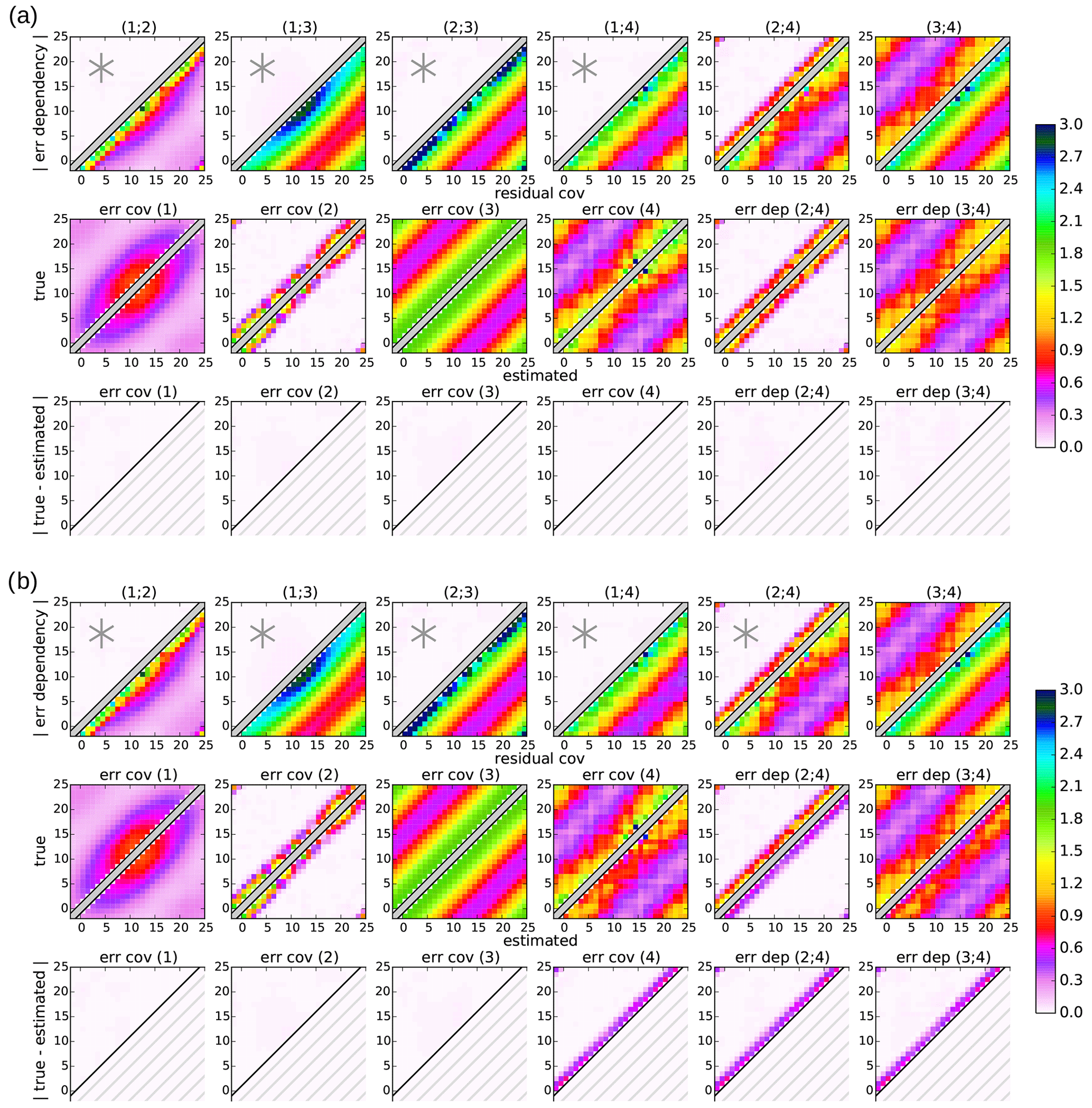
Figure 2 Experiment 1: covariance matrices for four datasets (I=4) with true dependencies of datasets (2; 4) and (3; 4). Datasets (1; 2; 3) build the basic triangle. Dataset 4 is estimated (a) from its reference dataset 1 (sequential estimation) and (b) from an additional independent triangle (1; 2; 4) (triangular estimation). For each subplot, gray asterisks in the upper-left part of the first row indicate that these error dependencies are assumed to be zero in the estimation. Note that the lower-right part of each subplot in the third row does not contain any data.

5.1 Uncertainties in additional dependencies

Figure 2 shows the error statistics of the first experiment in which only true error dependencies are generated between datasets (2;4) and (3;4) (upper-left part of the first row in Fig. 2a and b). This is in accordance with the estimation from the first setup shown in Fig. 2a that assumes independence in the basic triangle $(\mathrm{1};\mathrm{2};\mathrm{3})$ and between datasets (1;4) (independence assumptions indicated by gray asterisks). In contrast, the second setup shown in Fig. 2b requires an independence assumption between datasets (2;4) which is violated in this experiment. Thus, this experiment demonstrates the effects of uncertainties in this additional assumption.

By construction, the true error dependency matrices within the basic triangle – i.e., between (1;2), (1;3), and (2;3) – and along the sequential estimation between (1;4) are zero in this experiment (upper-left part of the first row, columns 1–4 in Fig. 2a and b). Because the first setup only assumes independence of these dataset pairs, it is able to estimate all four error covariance matrices and the two error dependency matrices between (2;4) and (3;4) accurately. Thus, the estimated error statistics exactly match the true ones (second row in Fig. 2a) and their absolute difference is zero (upper-left part of the third row in Fig. 2a).

In contrast, the additional triangular estimate in the second setup assumes an additional independence between datasets (2;4) which is not fulfilled. This neglected error dependency affects the triangular estimation of the error covariances of dataset 4, which is underestimated by half the neglected dependency as given in Eq. (45). This agrees with the experimental results shown in Fig. 2b: the neglected error dependency (2;4) with diagonal values around 1.2 (orange colors in upper-left part of the first row, column 5) induces an absolute uncertainty in the estimated error covariance 4 with diagonal values of around 0.6 (purple colors in the third row, column 4). The sign of the uncertainty that corresponds to the underestimation can be seen by comparing the true and estimated error covariances matrices of dataset 4 (second row, column 4). This uncertainty in the error covariance estimate of dataset 4 also affects the subsequent estimates of the error dependencies (2;4) and (3;4) which are expected to transfer the uncertainty in the error covariances with the same amplitude as given in Eq. (57). This can be confirmed by Fig. 2b: the uncertainties in the two estimated error dependencies equal the uncertainty in error covariance 4 (third row, columns 4–6) and, thus, the dependency estimates are underestimated by half the neglected dependency (2;4) (sign of uncertainty visible in the second row, columns 5 and 6).

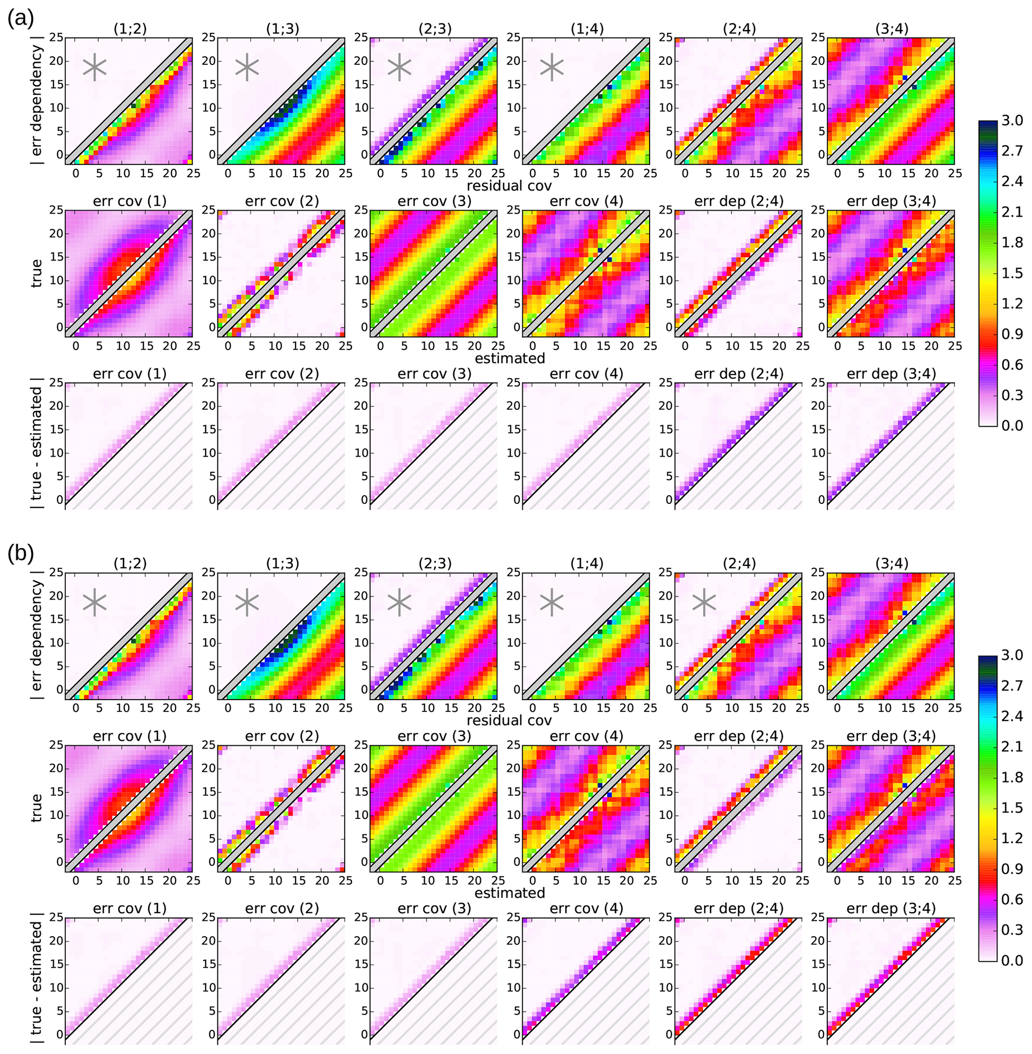
Figure 3 Experiment 2: covariance matrices for four datasets (I=4) with true dependencies of datasets (2; 3), (2; 4), and (3; 4). This figure is the same as Fig. 2 but with a neglected dependency in the basic triangle between datasets (2; 3).

This experiment demonstrates the potential to accurately estimate complete error covariances and some dependencies for more than three datasets if the underlying assumptions are sufficiently fulfilled. Note that this accurate estimation is independent of the complexity of the statistics like spatial variations or correlations. It also shows that an inaccurate independence assumption in an error covariance – here in the additional triangular estimation – may introduce uncertainties in all subsequent estimates of error covariances and dependencies, which is in accordance with the theoretical formulations above. The comparison of the two setups demonstrates the advantage of the sequential estimation for more than three datasets compared with only using triangular estimations.

Figure 4 Experiment 3: covariance matrices for four datasets (I=4) with true dependencies of datasets (2; 3), (2; 4), and (3; 4). This figure is the same as Fig. 2 but with an increased dependency in the basic triangle between datasets (2; 3).

5.2 Small uncertainties in the basic triangle

Figures 3 and 4 show the error statistics of the second and third experiments, respectively, where the independence assumption in the basic triangle is violated by introducing a nonzero dependency between datasets (2;3). The remaining true error statistics are the same as in the first experiment. Thus, in total, both experiments have three nonzero error dependencies between datasets (2;3), (2;4), and (3;4), and the neglected dependency (2;3) is increased from experiment two to experiment three (upper-left part of the first row in Figs. 3 and 4). These experiments demonstrate the effects of uncertainties in the basic triangle on the error estimates with the two setups.

Because both setups use the independent triangle $(\mathrm{1};\mathrm{2};\mathrm{3})$, the nonzero error dependency (2;3) violates this independence assumption and induces the same uncertainties in the error covariance estimates for both setups (see Eq. 45). Comparing the estimated error covariance matrices of datasets 1, 2, and 3 with the true matrices in Fig. 3a and b shows that all three matrices are similarly affected. While the magnitude of uncertainties is the same (third row, columns 1–3), their sign differs between the datasets, which is in accordance with Eq. (45). For the two datasets involved (2 and 3), the neglected positive dependency (2;3) is transferred with the same sign, leading to an underestimation of their error covariances (second row, columns 2 and 3). In contrast, the impact on the error covariance of the remaining dataset in the triangle (dataset 1) is reversed, leading to an overestimation of the true error covariance (second row, column 1). As expected from Eq. (45), the magnitude of uncertainty in the three estimated error covariances with diagonal elements around 0.4 (light-purple colors in the third row, columns 1–3) is half the neglected error dependency with diagonal elements around 0.2 (dark-purple colors in upper-left part of the first row, column 3).

The two setups differ with respect to the estimation of the error covariance of dataset 4, which affects the estimated dependencies (2;4) and (3;4), as described in the first experiment. For the sequential estimation of error covariance 4 in Fig. 3a (the first setup), the uncertainty in its reference error covariance 1 is transferred with same amplitude but the opposite sign (see Eq. 54), resulting in an underestimation of the error covariance matrix 4 (second and third rows, column 4). For the additional triangular estimation from $(\mathrm{1};\mathrm{2};\mathrm{4})$ in Fig. 3b (the second setup), the uncertainty in error covariance 4 remains the same as the first experiment, in which the independent triangle was accurate (second and third rows, column 4 of Fig. 3b vs. Fig. 2b). This is because the accuracy of a triangular estimation of an error covariance is only dependent on the assumed error dependencies between the dataset pairs – which are accurate in this experiment – but not on the other error covariance estimates (see Eq. 45).

For both setups, the uncertainties in the two estimated error dependencies (2;4) and (3;4) are the sum of the uncertainties in the error covariance estimates of the two datasets involved, i.e., (2;4) and (3;4), respectively. For the first setup in Fig. 3a, the two error dependencies are underestimated by the same amplitude as the neglected error dependency (2;3) (upper-left part of the first row, column 3 vs. the second and third rows, columns 5 and 6) because of its impact on both error covariance estimates, with a half amplitude each (second and third rows, columns 2–4). For the second setup in Fig. 3b, the two estimated error dependencies (2;4) and (3;4) are affected by both neglected error dependencies (2;3) and (2;4) due to their impact on the two error covariance estimates involved (2;4) and (3;4), respectively. Because the two uncertainties in the error covariances sum up, the estimated error dependencies are underestimated by half the sum of the two neglected error dependencies (upper-left part of the first row, columns 3 and 5 vs. the second and third rows, columns 5 and 6).

Consequently, the sequential estimation of the additional dataset 4 is more accurate in this experiment because the uncertainties in the basic triangle $(\mathrm{1};\mathrm{2};\mathrm{3})$ are smaller than the uncertainty in the assumed dependency (2;4) required for the additional triangular estimation, which can also be seen from Eq. (61).

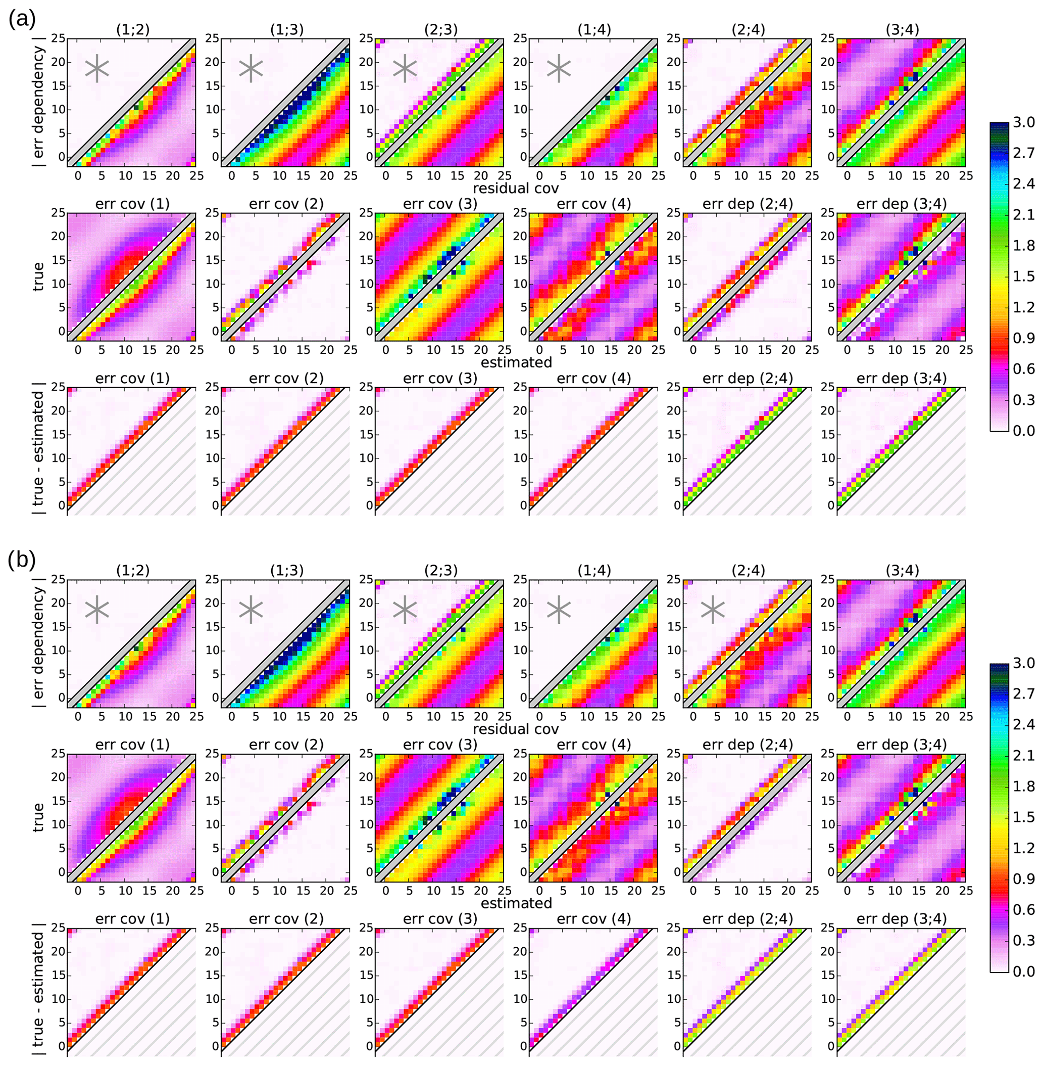
5.3 Large uncertainties in the basic triangle

This changes in the third experiment in Fig. 4, where the neglected dependency (2;3) in the basic triangle is larger than the neglected dependency (2;4) (upper-left parts of the first row, columns 3 and 5). Note that the increased error dependency (2;3) is even larger than the true error covariance 2 in some locations (upper-left parts of the first row, column 5, and second row, column 2). For the first setup in Fig. 4a, it can be seen that the increased uncertainty in the error covariance estimates in the basic triangle affects the estimates of all error statistics; the uncertainty in all estimated error statistics is increased proportionally to the increase in the neglected error dependency (2;3). As in the second experiment, the uncertainty amplitude is half the neglected error dependency for all error covariance estimates and equals the neglected error dependency for the estimated error dependencies (2;4) and (3;4) (upper-left part of the first row, column 3, and the third row of Fig. 4a vs. Fig. 3a).

The same holds for the error covariance estimates in the basic triangle $(\mathrm{1};\mathrm{2};\mathrm{3})$ in the second setup in Fig. 4b. In contrast, the additional triangular estimation of the error covariances of dataset 4 again remains the same as in the other two experiments. Because the independence assumption in the additional triangle $(\mathrm{1};\mathrm{2};\mathrm{4})$ is more accurate than the basic triangle $(\mathrm{1};\mathrm{2};\mathrm{3})$ in this experiment, the additional triangular estimation of error covariance 4 is more accurate than the sequential estimation (second and third rows, column 4 of Fig. 4a and b). If the other two error covariances 1 and 2 had also been estimated from the additional triangle $(\mathrm{1};\mathrm{2};\mathrm{4})$ instead of the basic triangle $(\mathrm{1};\mathrm{2};\mathrm{3})$, their estimation would also be more accurate (not shown).

The more accurate error covariance estimate of dataset 4 with the second setup also leads to more accurate estimates of the two error dependencies (2;3) and (3;4) due to the summation of the two error covariance estimates involved (second and third rows, columns 5 and 6 of Fig. 4a and b). In this particular example, the uncertainty in the error dependency (2;4) is even larger than the true dependency (upper-left parts of the first and third rows, column 5 of Fig. 4a and b), leading to negative dependencies for both estimates (lower-right part of the second row, column 5 of Fig. 4a and b). Similarly, the estimated error dependence matrix (3;4) loses its diagonal dominance: the diagonal elements are almost zero, but the more distant dependencies remain positive and similar to the true values (lower-right part of the second row, column 6 of Fig. 4a and b). This behavior is caused by the different spatial correlation scales of the two datasets 3 and 4 and might give an indication of inaccurate assumptions in real applications. Note that the error dependency (2;4) estimated with the second setup is more accurate in this experiment, despite its inconsistency concerning the assumption of zero error dependency (2;4) in the estimation of error covariance 4. However, due to their negative dependency estimates, the independence assumption would be more accurate than the actual estimates from both setups in this case.

The large variation in the uncertainties in the error estimates from the two setups among the different experiments demonstrates the importance of selecting an appropriate setup for the error estimation problem, which will be discussed in Sect. 6.2.

6 Conceptual summary and guidelines

This section provides a summary of the statistical error estimation method proposed in this study, with focus on its technical application. Section 6.1 summarizes the general assumptions and provides rules for the minimal conditions to solve the problem, including an illustrative visualization. Section 6.2 formulates guidelines for the selection of an appropriate setup of datasets under imperfect assumptions. Algorithmic summaries of the calculation of error statistics from residual covariances and cross-covariances, respectively, are given in Appendix A.

6.1 Minimal conditions

This section provides a conceptual discussion of different conditions that need to be fulfilled in order to be able to solve the error estimation problem. The discussion is based on the previous sections, but it is formulated in a qualitative way without providing mathematical details.

For error statistics that need to be assumed, their specific formulation may have different forms. The easiest and most common assumption is to set their error correlations and, thus, the error cross-covariances and dependencies to zero. This assumption (used in Sect. 4.1 and 4.2) is equivalent to the 3CH and TC methods. However, any nonzero error statistics can be defined and used in the general form, which is summarized in Appendix A. This also includes assuming error statistics as a function of other error statistics, including the ones estimated during the calculation. The only restriction is that all assumed error statistics must be fully determined by other error statistics or predefined values.

The number of error statistics that can be estimated for a given number of datasets (N_I) has been introduced in Sect. 2. However, not every possible choice of error statistics to be estimated provides a solution, which was also observed by Vogelzang and Stoffelen (2021) in the scalar case. The following discussion only considers setups in which all error covariances and as many error cross-statistics as possible are estimated.

In the first step, some error covariances need to be estimated directly “from scratch”, i.e., with no other error covariances available. Given the basic formulation of residual covariances in Eq. (20), a single error covariance (C_i) can only be eliminated when the other one (C_j) is replaced. Because every replacement of an error covariance of the same form introduces another error covariance, all other error covariances can only be removed if the final replacement again introduces the initial error covariance (C_i).

However, the resulting equation that involves a closed series of residuals cannot always be solved for the initial error covariance. For less than three residuals involved (F<3), the estimation of error covariances requires additional assumptions (see Sect. 2). Because of the changing sign of error covariances in the equation, the initial error covariance (${\mathbf{C}}_{\stackrel{\mathrm{̃}}{i}}$) cancels out and cannot be eliminated if the number of involved residuals is even (see Sect. 3.3.1). Note that the equation could then be used to estimate one error dependency; thus, the number of estimated error statistics remains consistent with Sect. 2.

In addition, the error cross-covariances or dependencies between each involved dataset pair have to be assumed in order to close the estimation problem. Thus, the initial error covariance can only be estimated from a closed series of F datasets, along which each pair of error cross-covariances or dependencies (${\mathbf{D}}_{\stackrel{\mathrm{̃}}{i_f};\stackrel{\mathrm{̃}}{i_{f+\mathrm{1}}}}$, ${\mathbf{D}}_{\stackrel{\mathrm{̃}}{i_F};\stackrel{\mathrm{̃}}{\mathrm{1}}}$) has to be assumed and the number of involved datasets (F) is odd and larger than or equal to three (see Sect. 4.2.1).

In the second step, all remaining error covariances can be estimated sequentially from their residual to a prior dataset – denoted as the reference dataset – with previously estimated error covariance (see Sect. 4.2.2). This estimation also requires the assumption of the error cross-covariances or dependencies related to the residuals involved. Finally, the error cross-statistics, which are not required in the estimation of error covariances (A_I>0), can be estimated from their respective residual covariances (see Sect. 4.2.3).

Based on this, two general rules for the setup of datasets can be formulated that ensure the solvability of the problem in the case that all error covariances and as many error cross-statistics as possible (cross-covariances or dependencies) are estimated:

• (i)

  all error cross-statistics along a closed series of dataset pairs, for which the number of involved datasets is odd and larger than or equal to three, are needed (this closed series of datasets is called the “basic polygon” or “basic triangle” in the case of three datasets) and

• (ii)

  at least one error cross-statistic of each additional dataset to any prior datasets is needed (this prior dataset is called the “reference dataset” of the additional dataset).

Previously, Vogelzang and Stoffelen (2021) observed that some setups for four or five datasets do not produce a solution for the problem, but they did not discuss the general requirements. Limited solvability was also found by Gruber et al. (2016) for four datasets, but they developed an unnecessarily strong requirement that each dataset has to be part of an independent triangle.

An illustrative example of assumed dependencies for I=10 datasets is visualized in Fig. 5. Note that this is one of many possible setups that are determined by the two rules above. First, the error dependencies among three datasets (1; 2; 3) need to be assumed (basic triangle). Then, one error dependency of each additional dataset i>3 to any prior dataset j (with j<i) is assumed (sequential estimation). Alternatively, the basic triangle could be replaced, for example, by a basic polygon of five datasets (basic pentagon: 1; 2; 3; 5; 4) if the dependency (3; 5) is assumed instead of the dependency (3; 1).

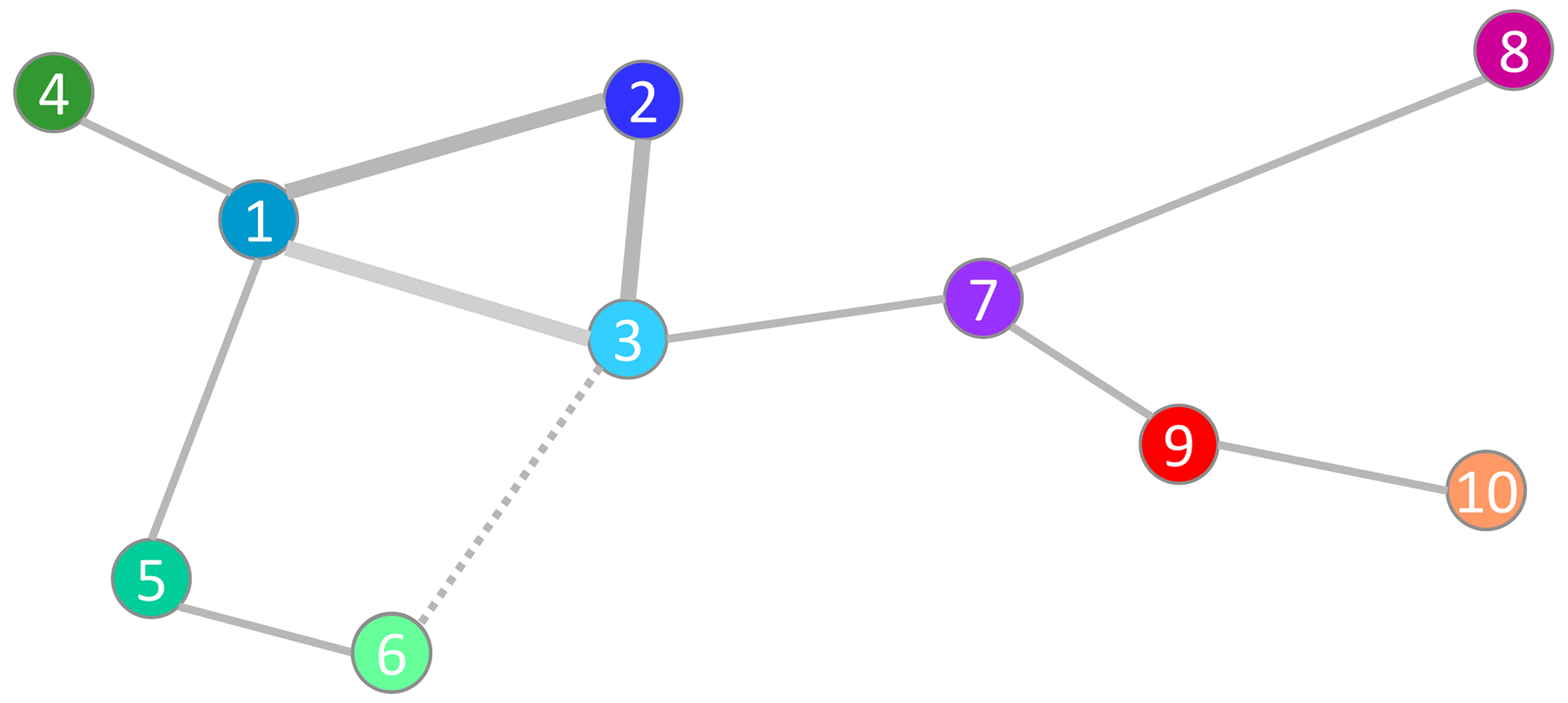
Figure 5 Independence tree: illustrative example of assumed error dependencies (gray lines) between 10 datasets (colored dots). The assumed dependencies in the basic triangle (1; 2; 3) are indicated by thicker lines. An alternative setup with a basic pentagon is indicated using the dotted line (3; 6) instead of the lighter gray line (1; 3).

6.2 Selection of the setup

The general rules given in Sect. 6.1 allow for multiple different setups of datasets that all solve the error estimation problem. However, in real applications, there might be significant differences in estimated error statistics from different setups as observed by studies such as Vogelzang and Stoffelen (2021) in the scalar case. The optimal selection is specific for each application and may depend on several requirements related to the actual purpose or use (e.g., available knowledge or accuracy of each estimate). This section provides some general guidelines on the selection of an appropriate setup among the various possible solutions with respect to the uncertainties introduced by statistical assumptions.

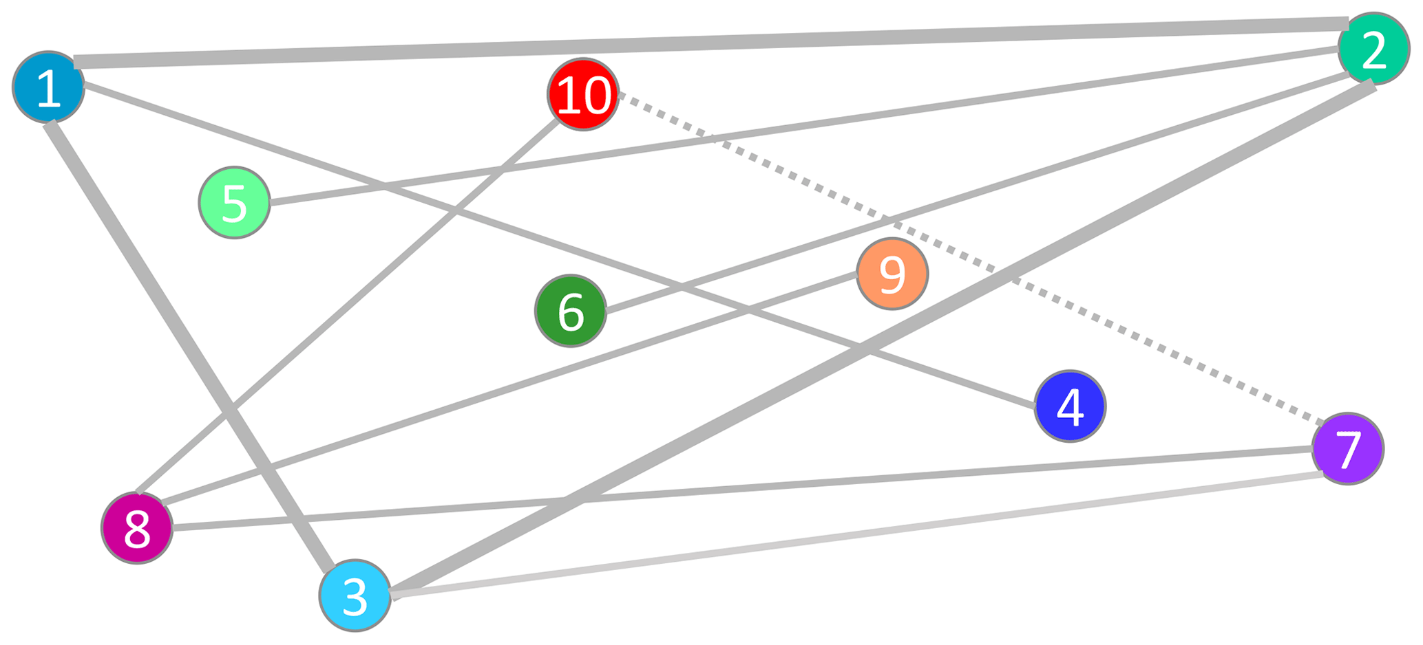
Figure 6 Improved independence tree: the same as Fig. 5 but with a modified setup for more accurate error estimates. Distances between datasets represent the accuracy of assumed dependencies between the error statistics. While locations are the same, the numbers and colors of the datasets have been changed according to the modified setup. An alternative setup with an additional independent triangle is indicated using the dotted line (7; 10) instead of the lighter gray line (3; 7).

The relative accuracy of an error covariance estimate is proportional to the ratio between the residual covariance Γ_i;j and the absolute uncertainty $\mathrm{\Delta }{\mathbf{D}}_{\stackrel{\mathrm{̃}}{i};\stackrel{\mathrm{̃}}{j}}$ of the assumed error dependency, which can be interpreted as being similar to a signal-to-noise ratio. In other words, the larger the residual covariance and the better the absolute estimate of the error dependency to the reference dataset, the more accurate the estimated error covariance. Because uncertainties in the error estimate do not necessarily sum up for a large basic polygon or along a branch of the independence tree (see Sect. 4.2.4), a large residual-to-dependency ratio with respect to the assumed cross-statistics is more important than a low number of intermediate datasets. In order to achieve sufficiently accurate estimates, the setup of datasets should be selected according to the expected accuracy of the estimated dependencies that minimize the residual-to-dependency ratio for each dataset:

$$\begin{array}{}\text{(62)}& \begin{array}{rl}& {\text{max}}_j\left({\displaystyle \frac{{\mathbf{\Gamma }}_{i;j}}{\mathrm{\Delta }{\mathbf{D}}_{\stackrel{\mathrm{̃}}{i};\stackrel{\mathrm{̃}}{j}}}}\right):j\to \text{ref}\left(i\right)\\ ⟺& {\text{min}}_j\left(\mathrm{\Delta }{\mathit{\rho }}_{\stackrel{\mathrm{̃}}{i};\stackrel{\mathrm{̃}}{j}}\right):j\to \text{ref}\left(i\right),\forall i.\end{array}\end{array}$$

The maximal residual-to-dependency ratio is equivalent to the minimal uncertainty in the normalized error correlations $\mathrm{\Delta }{\mathit{\rho }}_{\stackrel{\mathrm{̃}}{i};\stackrel{\mathrm{̃}}{j}}:=\frac{\mathrm{\Delta }{\mathbf{D}}_{\stackrel{\mathrm{̃}}{i};\stackrel{\mathrm{̃}}{j}}}{\sqrt{{\mathbf{C}}_{\stackrel{\mathrm{̃}}{i}}{\mathbf{C}}_{\stackrel{\mathrm{̃}}{j}}}}$. For example, if the error correlation of one dataset to another is known to some degree of accuracy, this dataset is well suited for use as a reference dataset. If assumed error dependencies are set to zero, the dataset to which the independence assumption is most certain should be selected as the reference dataset. Supposing that distances between datasets indicate their expected degree of independence in the independence tree, the setup visualized in Fig. 5 is not an appropriate selection. An example of an alternative setup that is expected to provide more accurate error estimates is shown in Fig. 6.

While uncertainties in the basic polygon only contribute half to the subsequent uncertainties, they affect the estimations of error statistics of all subsequent datasets (see Sect. 4.1.3 and 4.2.4 and Sect. 5.2 and 5.3). This has two implications. Firstly, the basic polygon, which is defined as the closed series of datasets that have the smallest error correlations, produces the smallest overall uncertainty with respect to all error estimates. Ideally, the basic polygon should be set as a closed series of datasets that have high pairwise independence or at least reasonably small dependencies among each pair. Secondly, if another pairwise independent polygon can be assumed for an additional dataset with similar accuracy to the dependency to its reference dataset, the additional error estimate may be more accurate using the direct estimation from this additional pairwise independent polygon rather than the sequential estimation (see Sects. 4.2.5 and 5.3). The additional pairwise independent polygon does not need to be connected to the basic polygon and may also have multiple independent branches, thus acting as an additional basic polygon. For example, in the setup shown in Fig. 6, the estimation of dataset 7 is sensitive to the dependency (3; 7) to its reference dataset and to dependencies in the basic triangle (1; 2; 3). If the dependency (7; 10) could be assumed with higher accuracy than these dependencies, the error covariances of dataset 7 can alternatively be calculated from the independent triangle (7; 8; 10) and the independence assumption between (3; 7) can be dropped. Thus, multiple independence trees can be defined around multiple separated basic triangles or basic polygons.

Furthermore, it is also possible to average the estimated error statistics of a dataset from multiple pairwise independent polygons, similar to an application of the N-cornered hat method (N-CH, e.g., Sjoberg et al., 2021) for an arbitrary subset of datasets. This setup builds an overestimated problem that requires the assumption of more error dependencies than the minimal requirements (see Sects. 2 and 6.1). However, it might be beneficial if multiple pairwise independent polygons containing the same dataset could be estimated with similar accuracy. In this case, potential uncertainties in the assumptions are expected to be reduced by the average over similar accurate estimates. Moreover, an extension to weighted averages of different estimations is possible, where the weights reflect the expected accuracy of each estimation formulation with respect to the others.

7 Conclusions

Despite the generalized matrix formulation, the main features of the presented approach are (i) its generality defining a flexible setup for any number of datasets according to the specific application, (ii) its optimality with respect to a minimal number of assumptions required, and (iii) its suitability to include expected nonzero dependencies between any pair of datasets. In contrast, the scalar N-CH method (N-cornered hat method) averages all estimates of each dataset, which is equivalent to assuming that the independence assumption among each dataset triplet is fulfilled with the same accuracy. However, this is not the case for most applications to geophysical datasets. For example, Rieckh et al. (2021) applied the N-CH method to multiple atmospheric model and observational datasets and discussed neglected levels of independence between different datasets, which are expected to vary significantly. Pan et al. (2015) tried to account for such variations by clustering the datasets into structural groups; however, this approach requires more assumptions than necessary and makes the result highly sensitive to the selected grouping. In contrast, the method presented here provides an optimal and flexible approach to handle multiple datasets with different levels of expected independence. Depending on the specific application, the estimation may be based on the minimal number of assumptions required or a (weighted) average over any number of estimations with similar expected accuracies.

An important application of the presented method is expected to be numerical weather prediction (NWP), where short-term forecasts from multiple national centers can be used to estimate the error statistics required for data assimilation. In contrast to previous statistical methods, potential dependencies among the forecasts, i.e., due to the assimilation of similar observations, can be considered in the error estimation and even explicitly quantified. Future work will show how this statistical approach compares to state-of-the-art background error estimates based on computationally expensive Monte Carlo-based or ensemble-based methods. While the presented method can be formulated to provide symmetric error covariances, a risk remains that negative values might occur for real applications due to inaccurate assumptions or sampling uncertainties.

In comparison to a posteriori methods that statistically estimate optimal error covariances for data assimilation, an a priori error estimation of collocated datasets has three main advantages: (i) optimal error statistics are calculated analytically without requiring an iterative minimization including multiple executions of the assimilation, (ii) complete covariance matrices provide spatially resolved fields of error statistics at each collocated location including spatial- and cross-species correlations, and (iii) error statistics of all datasets are estimated without selecting one dataset as a reference. This enables the consideration of more than two datasets in the assimilation. Given sufficiently estimated error statistics, the final analysis with respect to all datasets will be closer to the truth than any analysis between two datasets only. Thus, the rapidly increasing number of geophysical observations and model forecasts enable improved analyses due to increasingly overlapping datasets, and the optimal error statistics can be calculated, for example, with the method presented here. Specifically, the possibility to estimate optimal error cross-covariances between datasets provides important information for data assimilation, in which the violation of the independence assumption remains a major challenge (Tandeo et al., 2020).

However, current data assimilation schemes are not suited for multiple overlapping datasets, and cross-errors between datasets are assumed to be negligible. In contrast, the statistical error estimation method presented in this study is explicitly tailored to multiple datasets that cannot be assumed to be independent. Thus, the estimated error covariances are not consistent with assimilation algorithms assuming (two) independent datasets. If the estimated error dependencies among all assimilated datasets are small, the independence assumption may be regarded as sufficiently fulfilled. The error estimation method then provides error covariances for assimilation and information on the accuracy of the independence assumption. Otherwise, generalized assimilation schemes need to be developed for a proper use of this additional statistical information in data assimilation. Although this increases complexity, such generalized assimilation schemes enable fundamental improvements in terms of an optimal analysis from multiple datasets with respect to their error covariances and cross-statistics.

Appendix A: Algorithms

The general estimation procedure of error statistics for I≥3 datasets is summarized in Algorithms A1 and A2. The algorithms require residual covariances or cross-covariances among all I datasets (calculated from residual statistics) and I assumed error dependencies or cross-covariances, respectively. Based on this, the first error covariance matrix is calculated with a polygonal estimation. Then, error statistics of the remaining datasets are calculated sequentially in an iterative procedure: introducing a new dataset i with given residual statistics (covariances or cross-covariances) to dataset ref(i) for each $i\in [\mathrm{2},I]$ with ref(i)<i. Note that this is equivalent to a direct estimation of all error covariances in the basic polygon and a sequential estimation of the additional error covariances of datasets i>F (see Sect. 4.2.5).

Algorithm A1 Iterative calculation of error covariances and dependencies for I datasets from residual covariances with a general basic polygon of F≤I datasets.

Require:

$\mathtt{\text{rescov}}(i;\text{ref}(i);:;:)\forall i\in [\mathrm{2},I],\mathtt{\text{rescov}}(\text{F};\mathrm{1};:;:)$

Require:

$\mathtt{\text{errdep}}(i;\text{ref}(i);:;:)\forall i\in [\mathrm{2},I],\mathtt{\text{errdep}}(\text{F};\mathrm{1};:;:)$

– first dataset –

$\begin{array}{lll}\mathtt{\text{errcov}}(\mathrm{1};:;:)\leftarrow \mathrm{0.5}& \cdot \left[\right({\sum }_{f=\mathrm{1}}^{F-\mathrm{1}}(-\mathrm{1}{)}^{f-\mathrm{1}}\cdot \mathtt{\text{rescov}}(\text{f+1};\text{f};:;:\left)\right)+\mathtt{\text{rescov}}(\text{F};\mathrm{1};:;:)& \\ & +\left({\sum }_{f=\mathrm{1}}^{F-\mathrm{1}}\right(-\mathrm{1}{)}^{f-\mathrm{1}}\cdot \mathtt{\text{errdep}}(\text{f+1};\text{f};:;:))+\mathtt{\text{errdep}}(\text{F};\mathrm{1};:;:\left)\right]& \mathit{\{}\sim \mathit{\text{Eq. (29)}}\mathit{\}}\end{array}$

– loop over datasets –

for $i=\mathrm{2},I$ do

$\mathtt{\text{errcov}}(i;:;:)\leftarrow \mathtt{\text{rescov}}(i;\text{ref}(i);:;:)+\mathtt{\text{errdep}}(i;\text{ref}(i);:;:)-\mathtt{\text{errcov}}\left(\text{ref}\right(i);:;:)$        { ∼ Eq. (25)}

– remaining cross-statistics –

for $j=\mathrm{1},i-\mathrm{1}$ do

if j≠ref(i) then

$\mathtt{\text{errdep}}(i;j;:;:)\leftarrow \mathtt{\text{errcov}}(i;:;:)+\mathtt{\text{errcov}}(j;:;:)-\mathtt{\text{rescov}}(i;j;:;:)$        { ∼ Eq. (30)}

end if

$\mathtt{\text{errdep}}(j;i;:;:)\leftarrow \mathtt{\text{errdep}}(i;j;:;:)$        {∼ Eq. (14)}

end for

end for

Algorithm A2 Iterative calculation of error covariances and cross-covariances for I datasets from residual cross-covariances with a basic triangle of three datasets.

Require:

$\mathtt{\text{rescross}}(i;\text{ref}(i);i;j;:;:),\mathtt{\text{rescross}}\left(\text{ref}\right(i);i;\text{ref}(i);j;:;:)\forall i\in [\mathrm{2},I],j\ne \text{ref}\left(i\right),j\ne i,\mathtt{\text{rescross}}(\mathrm{1};\mathrm{2};\mathrm{1};\mathrm{3};:;:)$

Require:

$\mathtt{\text{errcross}}(i;\text{ref}(i);:;:)\forall i\in [\mathrm{2},I],\mathtt{\text{errcross}}(\mathrm{1};\mathrm{3};:;:)$

for $i=\mathrm{2},I$ do

$\mathtt{\text{errcross}}\left(\text{ref}\right(i);i;:;:)\leftarrow \mathtt{\text{errcross}}(i;\text{ref}(i);:;:{)}^{\mathrm{T}}$        {∼ Eq. (10)}

end for

– first dataset –

$\mathtt{\text{errcov}}(\mathrm{1};:;:)\leftarrow \mathtt{\text{rescross}}(\mathrm{1};\mathrm{2};\mathrm{1};\mathrm{3};:;:)+\mathtt{\text{errcross}}(\mathrm{1};\mathrm{3};:;:)+\mathtt{\text{errcross}}(\mathrm{2};\mathrm{1};:;:)-\mathtt{\text{errcross}}(\mathrm{2};\mathrm{3};:;:)$        {∼ Eq. (32)}

– loop over datasets –

for $i=\mathrm{2},I$ do

$\mathtt{\text{errcov}}(i;:;:)\leftarrow \mathtt{\text{rescross}}(i;\text{ref}(i);i;j;:;:)+\mathtt{\text{rescross}}\left(\text{ref}\right(i);i;\text{ref}(i);j;:;:)$

$-\mathtt{\text{errcov}}\left(\text{ref}\right(i);:;:)+\mathtt{\text{errcross}}(i;\text{ref}(i);:;:)+\mathtt{\text{errcross}}\left(\text{ref}\right(i);i;:;:)$        { ∼ Eq. (34)}

– remaining cross-statistics –

for $j=\mathrm{1},i-\mathrm{1}$ do

if j≠ref(i) then

$\mathtt{\text{errcross}}(i;j;:;:)\leftarrow \mathtt{\text{rescross}}\left(\text{ref}\right(i);i;\text{ref}(i);j;:;:)-\mathtt{\text{errcov}}\left(\text{ref}\right(i);:;:)$

$+\mathtt{\text{errcross}}\left(\text{ref}\right(i);j;:;:)+\mathtt{\text{errcross}}(i;\text{ref}(i);:;:)$        { ∼ Eq. (36)}

$\mathtt{\text{errcross}}(j;i;:;:)\leftarrow \mathtt{\text{errcross}}(i;j;:;:{)}^{\mathrm{T}}$        {∼ Eq. (10)}

end if

end for

end for

Algorithm A1 is formulated for symmetric statistic matrices, where the error covariances $\mathtt{\text{errcov}}(i;:,:)$ of each dataset i and the error dependency matrices $\mathtt{\text{errdep}}(i;j;:;:)$ between each pair (i;j) are estimated from symmetric residual covariances $\mathtt{\text{rescov}}(i;j:;:;)$. In this algorithm, the generalized formulation of a basic polygon of F≤I residuals, for any odd F≥3, is used for the estimation of the first error covariance. In Algorithm A2, the error covariance- and cross-covariance matrices $\mathtt{\text{errcross}}(i;j;:;:)$ of each pair (i;j) are estimated from the residual cross-covariances $\mathtt{\text{rescross}}(i;j;i;k;:;:)$ between ($i-j;i-k$). Here, the third dataset k in the residual cross-covariances can be freely selected and does not affect the accuracy of the estimates (see Sect. 4.2.4). This algorithm uses a basic triangle as an example for a basic polygon for the estimation of the first error covariance. Each operation is applied element-wise to each matrix-element indicated by the last two indices $(:;:)$, and matrices may contain different locations of the same quantity as well as different fields for multiple quantities of any dimension (multivariate covariances). Transposed matrices with respect to the two location indices are indicated by [ ]^T.

The equations relate to the general exact formulations, which require some error dependencies or cross-covariances to be given (see Sect. 3). The explicit calculation of the error cross-statistics (dependencies or cross-covariances) is not needed if only error covariances are of interest. In theory, both algorithms provide the same error estimations (see Sect. 3.2.3). The decision to estimate error statistics from residual covariances (Algorithm A1) or cross-covariances (Algorithm A2) depends on the availability of residual statistics; the need for symmetric estimations of error covariances, which is only intrinsically guaranteed in Algorithm A1; and the need to estimate asymmetric components of error cross-covariances, which can only be estimated with Algorithm A2 (see Sect. 3.3.1). Note that the generalized basic polygon can also be used for the estimation of the first error covariance in Algorithm A2.