Electron holes in a regularized kappa background

The pseudopotential method is used to derive electron hole structures in a suprathermal plasma with a regularized κ probability distribution function background. The regularized character allows the exploration of small κ values beyond the standard suprathermal case for which $\mathit{\kappa }>\mathrm{3}/\mathrm{2}$ is a necessary condition. We found the nonlinear dispersion relation yielding the amplitude of the electrostatic potential in terms of the remaining parameters, in particular the drift velocity, the wavenumber and the spectral index. Periodic, solitary wave, drifting and non-drifting solutions have been identified. In the linear limit, the dispersion relation yields generalized Langmuir and electron acoustic plasma modes. Standard electron hole structures are regained in the κ≫1 limit.

1 Introduction

The phenomenon of so-called electron holes in a plasma has received growing attention in the recent past, especially due to recent spacecraft observations of such structures; see, e.g., Steinvall (2019a, b). In particular, a recent study resolved the phase space density deficit of trapped electrons and proved that the solitary waves with bipolar profiles observed in space plasma are electron holes (Mozer, 2018). General reviews of electron holes can be found in Luque (2005) or Eliasson (2006). For the application to space plasmas, a quantitative treatment of electron holes should take into account the presence of a suprathermal, i.e., non-Maxwellian, background plasma. This was already pointed out in Schamel (2015, 2023) and carried out in Haas (2021), Aravindakshan (2018), Aravindakshan (2020) and Jenab (2021). In Haas (2021), the Maxwellian description of the trapped (hole) and untrapped (background) electron populations was substituted by one with a so-called standard kappa distribution (SKD).

The SKD is a simple generalization of a Maxwellian that was originally introduced by Olbert (1968) to describe non-Maxwellian power law distributions of suprathermal plasma species, which are frequently observed in solar wind (Lazar, 2017) and are formed via the interaction of solar wind particles with plasma turbulence (e.g., Ma and Summers, 1998; Yoon, 2014; Yoon et al., 2018), preventing a relaxation to a Maxwellian or bi-Maxwellian. Since then the SKD has been applied successfully to numerous space plasma and laboratory scenarios. Along with these successes, various limitations of the SKD were also identified: it exhibits diverging velocity moments, a positive lower limit of allowed kappa parameter values ($\mathit{\kappa }>\mathrm{3}/\mathrm{2}$) and a non-extensive entropy (for a recent overview, see Lazar, 2021). In addition, two types of SKDs were identified, i.e., the original one introduced by Olbert (1968) with a prescribed reference speed and a modified one that can be traced to Matsumoto (1972) with a temperature equal to that of the associated Maxwellian, and it was demonstrated (Lazar, 2016) that care has to be taken in selecting one of those for a given physical system. The kappa distribution was proposed in Vasyliunas (1968), and an extensive discussion of the different kappa distributions can be found in Pierrard (2010) and Hau (2007). In addition to these principal limitations of SKDs, there is also an observational one: SKDs do not allow one to describe velocity distributions which are harder than v⁻⁵. However, distributions with harder tails are actually observed: see, for example, Gloeckler et al. (2012). At the same time, these measurements also reveal that kappa values near 2 or below are frequently observed. This can also be seen for solar wind electrons: see, e.g., Pierrard (2022). Such low values of kappa imply unphysical features of the SKD as discussed in Scherer (2019). Another example is solar energetic particles: see, e.g., Oka et al. (2013). Kappa values as low as 1.63 and 2 are also obtained for particle distributions in the outer heliosphere (e.g., Heerikhuisen et al., 2008; Zirnstein et al., 2017). Finally, SKDs are not consistent with exponential cutoffs of observed power law distributions of suprathermal protons in the solar wind (Fisk and Gloeckler, 2012).

All of these complications in employing the SKD can be avoided when one uses the regularized kappa distribution (RKD) introduced non-relativistically in Scherer (2017) and for the relativistic case in HanThanh (2022). The RKD exhibits an exponential cutoff of the power at high velocities. Such a cutoff is a result of the fact that any acceleration process can only occur on a finite spatial scale and on a finite timescale. Consequently, such a power law cannot extend to infinity (as in the case of the standard kappa distribution) and must cut off. The main purpose of the present work is to adopt a regularized version of the SKD and to analyze the consequences. The RKD in particular removes all divergences in the theory and moves the lower limit for the kappa parameter to zero (Scherer, 2019). Both features have consequences for correspondingly described physical systems: in Yoon (2014) it was demonstrated that an “infrared catastrophe” is avoided when using the RKD instead of the SKD, and in Liu (2020) it was shown that extending the range of kappa values to zero broadens the possible properties of solitary ion acoustic waves in a plasma with RKD electrons. Here the reference value of κ is adopted according to Eq. (2) for the SKD.

Since the first generalization of the analytical treatment of electron holes in an equilibrium plasma to a suprathermal plasma was also achieved by employing an SKD (Haas, 2021), the same constraints remain: not all moments of the velocity distribution functions exist, and kappa has to be greater than $\mathrm{3}/\mathrm{2}$, thereby potentially preventing the study of a physically interesting regime because harder velocity distributions were observed (see, e.g., Gloeckler et al., 2012 and Pierrard, 2022) and were associated with observations of various solitary waves (Vasko, 2017). Therefore, the present work revisits the quantitative treatment of electron holes in a suprathermal plasma, where the electron velocity distribution is described with the RKD.

The structure of the paper is as follows: in Sect. 2 the one-dimensional RKD is defined, in Sect. 3 various dimensionless variables are introduced, in Sect. 4 the method of the pseudopotential is applied, and in Sect. 5 special solutions of the resulting Poisson equation are derived. After an analysis of the corresponding dispersion relation in Sect. 6 for homogeneous trapped electron distributions, the final Sect. 7 contains the conclusions of the study.

2 One-dimensional regularized κ distribution

The starting point (Scherer, 2019; Liu, 2020) is the three-dimensional isotropic RKD,

$$\begin{array}{}\text{(1)}& \begin{array}{rl}{f}_{\mathrm{3}}\left(\mathit{u}\right)=& {\displaystyle \frac{n_{\mathrm{0}}}{(\mathit{\pi }\mathit{\kappa }{\mathit{\theta }}^{\mathrm{2}}{)}^{\mathrm{3}/\mathrm{2}}U\left(\frac{\mathrm{3}}{\mathrm{2}},\frac{\mathrm{3}}{\mathrm{2}}-\mathit{\kappa },{\mathit{\alpha }}^{\mathrm{2}}\mathit{\kappa }\right)}}\\ & \times {\left(\mathrm{1}+{\displaystyle \frac{u^{\mathrm{2}}}{\mathit{\kappa }{\mathit{\theta }}^{\mathrm{2}}}}\right)}^{-\mathit{\kappa }-\mathrm{1}}\exp \left(-{\displaystyle \frac{{\mathit{\alpha }}^{\mathrm{2}}{u}^{\mathrm{2}}}{{\mathit{\theta }}^{\mathrm{2}}}}\right),\end{array}\end{array}$$

where n₀ is the equilibrium electron number density, κ>0 is the spectral index, θ is a reference speed, U is a Kummer function of the second kind (or Tricomi function) described in (Scherer, 2019; Liu, 2020; Abramowitz, 1972), u is the velocity vector with $u=\left|\mathit{u}\right|$, and α≥0 is the cutoff parameter.

In the non-regularized limit α→0, one regains the SKD:

$$\begin{array}{}\text{(2)}& \begin{array}{rl}{f}_{\mathrm{3}}\left(\mathit{u}\right)=& {\displaystyle \frac{n_{\mathrm{0}}\mathrm{\Gamma }(\mathit{\kappa }+\mathrm{1})}{(\mathit{\pi }\mathit{\kappa }{\mathit{\theta }}^{\mathrm{2}}{)}^{\mathrm{3}/\mathrm{2}}\mathrm{\Gamma }\left(\mathit{\kappa }-\frac{\mathrm{1}}{\mathrm{2}}\right)}}\\ & \times {\left(\mathrm{1}+{\displaystyle \frac{u^{\mathrm{2}}}{\mathit{\kappa }{\mathit{\theta }}^{\mathrm{2}}}}\right)}^{-\mathit{\kappa }-\mathrm{1}},\mathit{\alpha }\to \mathrm{0},\end{array}\end{array}$$

where Γ is the gamma function, which is positive-definite provided that $\mathit{\kappa }>\mathrm{1}/\mathrm{2}$. For the RKD, this constraint is not imposed on κ>0.

For the treatment of electrostatic structures, it is convenient to define the one-dimensional RKD. For this purpose we use cylindrical coordinates in velocity space and write $u^{\mathrm{2}}=v^{\mathrm{2}}+w^{\mathrm{2}}$, where v is the component of the velocity parallel to the electric field and w contains only the perpendicular velocity components, with $w=\left|\mathit{w}\right|$. In the isotropic case the one-dimensional RKD is

$$\begin{array}{}\text{(3)}& \begin{array}{rl}f\left(v\right)=& \mathrm{2}\mathit{\pi }\underset{\mathrm{0}}{\overset{\mathrm{\infty }}{\int }}\mathrm{d}ww{f}_{\mathrm{3}}\left(\mathit{u}\right)\\ =& {\displaystyle \frac{\mathrm{2}\mathit{\pi }{n}_{\mathrm{0}}{e}^{-\frac{{\mathit{\alpha }}^{\mathrm{2}}{v}^{\mathrm{2}}}{{\mathit{\theta }}^{\mathrm{2}}}}}{(\mathit{\pi }\mathit{\kappa }{\mathit{\theta }}^{\mathrm{2}}{)}^{\mathrm{3}/\mathrm{2}}U\left(\frac{\mathrm{3}}{\mathrm{2}},\frac{\mathrm{3}}{\mathrm{2}}-\mathit{\kappa },{\mathit{\alpha }}^{\mathrm{2}}\mathit{\kappa }\right)}}\\ & \times \underset{\mathrm{0}}{\overset{\mathrm{\infty }}{\int }}\mathrm{d}ww{\left(\mathrm{1}+{\displaystyle \frac{v^{\mathrm{2}}+w^{\mathrm{2}}}{\mathit{\kappa }{\mathit{\theta }}^{\mathrm{2}}}}\right)}^{-\mathit{\kappa }-\mathrm{1}}\\ & \times \exp \left(-{\displaystyle \frac{{\mathit{\alpha }}^{\mathrm{2}}{w}^{\mathrm{2}}}{{\mathit{\theta }}^{\mathrm{2}}}}\right)\\ =& {\displaystyle \frac{n_{\mathrm{0}}({\mathit{\alpha }}^{\mathrm{2}}\mathit{\kappa }{)}^{\mathit{\kappa }}{e}^{{\mathit{\alpha }}^{\mathrm{2}}\mathit{\kappa }}}{(\mathit{\pi }\mathit{\kappa }{\mathit{\theta }}^{\mathrm{2}}{)}^{\mathrm{1}/\mathrm{2}}U\left(\frac{\mathrm{3}}{\mathrm{2}},\frac{\mathrm{3}}{\mathrm{2}}-\mathit{\kappa },{\mathit{\alpha }}^{\mathrm{2}}\mathit{\kappa }\right)}}\\ & \times \mathrm{\Gamma }\left[-\mathit{\kappa },{\mathit{\alpha }}^{\mathrm{2}}\mathit{\kappa }\left(\mathrm{1}+{\displaystyle \frac{v^{\mathrm{2}}}{\mathit{\kappa }{\mathit{\theta }}^{\mathrm{2}}}}\right)\right],\end{array}\end{array}$$

where here Γ is the incomplete gamma function of the indicated arguments (Abramowitz, 1972). In other words, f(v) comes from the three-dimensional version after integration over the two perpendicular velocity components.

In the non-regularized limit α→0, one regains the standard one-dimensional κ distribution (Summers, 1991; Podesta, 2005)

$$\begin{array}{}\text{(4)}& f\left(v\right)={\displaystyle \frac{n_{\mathrm{0}}\mathrm{\Gamma }\left(\mathit{\kappa }\right)}{(\mathit{\pi }\mathit{\kappa }{\mathit{\theta }}^{\mathrm{2}}{)}^{\mathrm{1}/\mathrm{2}}\mathrm{\Gamma }\left(\mathit{\kappa }-\frac{\mathrm{1}}{\mathrm{2}}\right)}}{\left(\mathrm{1}+{\displaystyle \frac{v^{\mathrm{2}}}{\mathit{\kappa }{\mathit{\theta }}^{\mathrm{2}}}}\right)}^{-\mathit{\kappa }},\mathit{\alpha }\to \mathrm{0},\end{array}$$

which is positive-definite provided that $\mathit{\kappa }>\mathrm{3}/\mathrm{2}$.

In the treatment of electrostatic structures, to satisfy Vlasov's equation, the distribution function is a function of the constants of motion. In the one-dimensional, time-independent case, the available constants of motion are given by

$$\begin{array}{}\text{(5)}& \mathit{ϵ}={\displaystyle \frac{m{v}^{\mathrm{2}}}{\mathrm{2}}}-e\mathit{\varphi },\mathit{\sigma }=\text{sgn}\left(v\right),\end{array}$$

where ϕ=ϕ(x) is the scalar potential, m is the electron mass, and −e is the electron charge. The sign of the velocity $\mathit{\sigma }=v/\left|v\right|$ is an additional constant of motion just in case of untrapped particles. The energy variable ϵ can be used to distinguish untrapped (ϵ>0) and trapped (ϵ<0) electrons.

Analogously to Schamel (1972, 2015, 2023) (where the background is not in the RKD form), presently one starts from Eq. (3), using for the untrapped part the replacement $v\to \mathit{\sigma }\sqrt{\mathrm{2}\mathit{ϵ}/m}+v_{\mathrm{0}}$, where v₀ is a drift velocity defining the distributions of untrapped and trapped electrons according to

$$\begin{array}{}\text{(6)}& {\displaystyle }\begin{array}{rl}f=& f(\mathit{ϵ},\mathit{\sigma })={\displaystyle \frac{A{n}_{\mathrm{0}}}{\mathit{\theta }}}\left(\mathrm{1}+{\displaystyle \frac{k_{\mathrm{0}}^{\mathrm{2}}\mathrm{\Psi }}{\mathrm{2}}}\right)\\ & \left[H\left(\mathit{ϵ}\right)\mathrm{\Gamma }\left(-\mathit{\kappa },{\mathit{\alpha }}^{\mathrm{2}}\mathit{\kappa }\left(\mathrm{1}+{\displaystyle \frac{\mathrm{1}}{\mathit{\kappa }{\mathit{\theta }}^{\mathrm{2}}}}(\mathit{\sigma }\sqrt{\mathrm{2}\mathit{ϵ}/m}+v_{\mathrm{0}}{)}^{\mathrm{2}}\right)\right)\right.\\ & \left.+H(-\mathit{ϵ})\mathrm{\Gamma }\left(-\mathit{\kappa },{\mathit{\alpha }}^{\mathrm{2}}\mathit{\kappa }\left(\mathrm{1}+{\displaystyle \frac{v_{\mathrm{0}}^{\mathrm{2}}}{\mathit{\kappa }{\mathit{\theta }}^{\mathrm{2}}}}\right)\right)\left(\mathrm{1}-{\displaystyle \frac{\mathit{\beta }\mathit{ϵ}}{m{\mathit{\theta }}^{\mathrm{2}}}}\right)\right],\end{array}\text{(7)}& {\displaystyle }A={\displaystyle \frac{({\mathit{\alpha }}^{\mathrm{2}}\mathit{\kappa }{)}^{\mathit{\kappa }}{e}^{{\mathit{\alpha }}^{\mathrm{2}}\mathit{\kappa }}}{(\mathit{\pi }\mathit{\kappa }{)}^{\mathrm{1}/\mathrm{2}}U\left(\frac{\mathrm{3}}{\mathrm{2}},\frac{\mathrm{3}}{\mathrm{2}}-\mathit{\kappa },{\mathit{\alpha }}^{\mathrm{2}}\mathit{\kappa }\right)}},\end{array}$$

where H(ϵ) is the Heaviside function. The quantities k₀ and Ψ are dimensionless variables proportional to the wavenumber of periodic oscillations and to the electrostatic field amplitude, respectively, as will be qualified in the following. In addition, β is a dimensionless quantity associated with the inverse temperature of the trapped electron distribution. Unlike singular distributions as in Schamel (2015, 2023, 2018) and Haas (2021), here the velocity-shifted hole distribution is assumed to be continuous at the separatrix (ϵ=0) and an analytic function of the energy for both trapped and untrapped electrons. These choices have been made in order to focus on the role of the cutoff parameter α instead of further aspects.

Figure 1 An illustration of the Schamel distribution (in arbitrary units and for the sech potential in Eq. 13 in Schamel, 1986) for the values $\mathit{\beta }=-\mathrm{0.9}$, k₀=1.0, ψ=1.0, κ=0.5 and γ=0.1 of the parameters used for the notation in Haas (2021).

In the non-regularized case, using

$$\begin{array}{}\text{(8)}& \left({\mathit{\alpha }}^{\mathrm{2}}\mathit{\kappa }{)}^{\mathit{\kappa }}\mathrm{\Gamma }\right(-\mathit{\kappa },{\mathit{\alpha }}^{\mathrm{2}}\mathit{\kappa }s)\to {\displaystyle \frac{s^{-\mathit{\kappa }}}{\mathit{\kappa }}},\mathit{\alpha }\to \mathrm{0},\mathit{\kappa }>\mathrm{0}\end{array}$$

for a generic argument s and

$$\begin{array}{}\text{(9)}& U\left({\displaystyle \frac{\mathrm{3}}{\mathrm{2}}},{\displaystyle \frac{\mathrm{3}}{\mathrm{2}}}-\mathit{\kappa },{\mathit{\alpha }}^{\mathrm{2}}\mathit{\kappa }\right)\to {\displaystyle \frac{\mathrm{\Gamma }(\mathit{\kappa }-\mathrm{1}/\mathrm{2})}{\mathrm{\Gamma }(\mathit{\kappa }+\mathrm{1})}},\mathit{\alpha }\to \mathrm{0},\mathit{\kappa }>\mathrm{1}/\mathrm{2},\end{array}$$

from Eq. (6), one obtains

$$\begin{array}{}\text{(10)}& \begin{array}{rl}f=& {\displaystyle \frac{n_{\mathrm{0}}(\mathrm{1}+k_{\mathrm{0}}^{\mathrm{2}}\mathrm{\Psi }/\mathrm{2})}{(\mathit{\pi }\mathit{\kappa }{\mathit{\theta }}^{\mathrm{2}}{)}^{\mathrm{1}/\mathrm{2}}}}{\displaystyle \frac{\mathrm{\Gamma }\left(\mathit{\kappa }\right)}{\mathrm{\Gamma }(\mathit{\kappa }-\mathrm{1}/\mathrm{2})}}\\ & \times \left[H\left(\mathit{ϵ}\right){\left(\mathrm{1}+{\displaystyle \frac{\mathrm{1}}{\mathit{\kappa }{\mathit{\theta }}^{\mathrm{2}}}}{\left(\mathit{\sigma }\sqrt{{\displaystyle \frac{\mathrm{2}\mathit{ϵ}}{m}}}+v_{\mathrm{0}}\right)}^{\mathrm{2}}\right)}^{-\mathit{\kappa }}\right.\\ & \left.+H(-\mathit{ϵ}){\left(\mathrm{1}+{\displaystyle \frac{v_{\mathrm{0}}^{\mathrm{2}}}{\mathit{\kappa }{\mathit{\theta }}^{\mathrm{2}}}}\right)}^{-\mathit{\kappa }}\left(\mathrm{1}-{\displaystyle \frac{\mathit{\beta }\mathit{ϵ}}{m{\mathit{\theta }}^{\mathrm{2}}}}\right)\right],\end{array}\end{array}$$

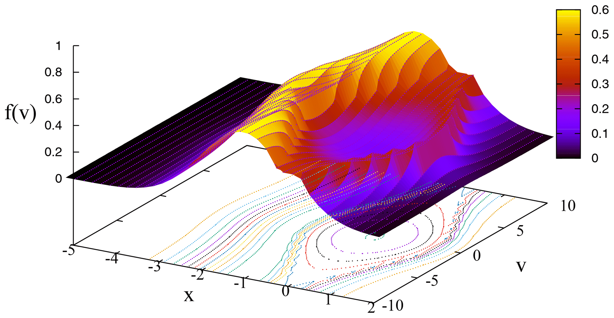
which is the κ version of Schamel's distribution that is given in its original form, e.g., in Eq. (4) in Schamel (1986) and illustrated in Fig. 1. A slight difference in comparison to the original formulation (Schamel, 1986, 2012) is that here the trapped electrons are described by a linear function of the energy instead of by a Maxwellian function.

Finally, the Poisson equation

$$\begin{array}{}\text{(11)}& {\displaystyle \frac{{\partial }^{\mathrm{2}}\mathit{\varphi }}{\partial x^{\mathrm{2}}}}={\displaystyle \frac{e}{{\mathit{\epsilon }}_{\mathrm{0}}}}(n-n_{\mathrm{0}}),n=n\left(\mathit{\varphi }\right)=\underset{-\mathrm{\infty }}{\overset{\mathrm{\infty }}{\int }}\mathrm{d}vf(\mathit{ϵ},\mathit{\sigma })\end{array}$$

is needed, where ε₀ is the vacuum permittivity. A uniform ionic background n₀ has been assumed.

3 Dimensionless variables

To avoid the use of a large number of parameters, it is convenient to adopt dimensionless variables. For the RKD, the question arises as to what the reference speed defining the velocity rescaling will be. It would be tempting to consider the use of a thermal speed v_T defined in terms of the averaged squared velocity, but this is a cumbersome expression containing Kummer functions,

$$\begin{array}{}\text{(12)}& \begin{array}{rl}{v}_T^{\mathrm{2}}& ={\displaystyle \frac{\langle u^{\mathrm{2}}\rangle }{\mathrm{3}}}={\displaystyle \frac{\mathrm{1}}{\mathrm{3}}}{\displaystyle \frac{\int d^{\mathrm{3}}u{u}^{\mathrm{2}}{f}_{\mathrm{3}}\left(\mathit{u}\right)}{\int d^{\mathrm{3}}u{f}_{\mathrm{3}}\left(\mathit{u}\right)}}\\ & ={\displaystyle \frac{\mathit{\kappa }{\mathit{\theta }}^{\mathrm{2}}}{\mathrm{2}}}{\displaystyle \frac{U\left(\frac{\mathrm{5}}{\mathrm{2}},\frac{\mathrm{5}}{\mathrm{2}}-\mathit{\kappa },{\mathit{\alpha }}^{\mathrm{2}}\mathit{\kappa }\right)}{U\left(\frac{\mathrm{3}}{\mathrm{2}},\frac{\mathrm{3}}{\mathrm{2}}-\mathit{\kappa },{\mathit{\alpha }}^{\mathrm{2}}\mathit{\kappa }\right)}},\end{array}\end{array}$$

the factor $\mathrm{1}/\mathrm{3}$ being introduced to comply with the one-dimensional geometry. Therefore, for the sake of simplicity, instead of the thermal speed, it is indicated to consider θ to be the reference speed. In this way, the rescaled variables are

$$\begin{array}{}\text{(13)}& \begin{array}{rl}& \stackrel{\mathrm{̃}}{x}={\displaystyle \frac{x}{\mathit{\lambda }}},\stackrel{\mathrm{̃}}{v}={\displaystyle \frac{v}{\mathit{\theta }}},\stackrel{\mathrm{̃}}{v_{\mathrm{0}}}={\displaystyle \frac{v_{\mathrm{0}}}{\mathit{\theta }}},\stackrel{\mathrm{̃}}{\mathit{\varphi }}={\displaystyle \frac{e\mathit{\varphi }}{m{\mathit{\theta }}^{\mathrm{2}}}},\\ & \stackrel{\mathrm{̃}}{n}={\displaystyle \frac{n}{n_{\mathrm{0}}}},\stackrel{\mathrm{̃}}{f}={\displaystyle \frac{f}{n_{\mathrm{0}}/\mathit{\theta }}},\stackrel{\mathrm{̃}}{\mathit{ϵ}}={\displaystyle \frac{\mathit{ϵ}}{m{\mathit{\theta }}^{\mathrm{2}}}},\end{array}\end{array}$$

where $\mathit{\lambda }=[{\mathit{ϵ}}_{\mathrm{0}}m{\mathit{\theta }}^{\mathrm{2}}/(n_{\mathrm{0}}{e}^{\mathrm{2}}){]}^{\mathrm{1}/\mathrm{2}}$ is a modified Debye length.

As discussed in Lazar (2016) in the non-regularized context, our standard choice of θ as a κ-independent parameter better fits a scenario with an enhanced tail in the velocity space. Alternatively, one could choose v_T from Eq. (12) to be κ-independent, which would be adequate for an enhanced core.

In dimensionless variables omitting for simplicity the tildes, the one-dimensional hole RKD from Eq. (6) is

$$\begin{array}{}\text{(14)}& \begin{array}{rl}f(\mathit{ϵ},\mathit{\sigma })=& A\left(\mathrm{1}+{\displaystyle \frac{k_{\mathrm{0}}^{\mathrm{2}}\mathrm{\Psi }}{\mathrm{2}}}\right)\\ & \times \left[H\left(\mathit{ϵ}\right)\mathrm{\Gamma }\left(-\mathit{\kappa },{\mathit{\alpha }}^{\mathrm{2}}\mathit{\kappa }\left(\mathrm{1}+{\displaystyle \frac{\mathrm{1}}{\mathit{\kappa }}}(\mathit{\sigma }\sqrt{\mathrm{2}\mathit{ϵ}}+v_{\mathrm{0}}{)}^{\mathrm{2}}\right)\right)\right.\\ & \left.+H(-\mathit{ϵ})\mathrm{\Gamma }\left(-\mathit{\kappa },{\mathit{\alpha }}^{\mathrm{2}}\mathit{\kappa }\left(\mathrm{1}+{\displaystyle \frac{v_{\mathrm{0}}^{\mathrm{2}}}{\mathit{\kappa }}}\right)\right)(\mathrm{1}-\mathit{\beta }\mathit{ϵ})\right],\end{array}\end{array}$$

while Poisson's Eq. (11) is

$$\begin{array}{}\text{(15)}& {\displaystyle \frac{{\partial }^{\mathrm{2}}\mathit{\varphi }}{\partial x^{\mathrm{2}}}}=n-\mathrm{1},n=n\left(\mathit{\varphi }\right)=\underset{-\mathrm{\infty }}{\overset{\mathrm{\infty }}{\int }}\mathrm{d}vf(\mathit{ϵ},\mathit{\sigma }),\end{array}$$

where $\mathit{ϵ}=v^{\mathrm{2}}/\mathrm{2}-\mathit{\varphi }$ and σ=sgn(v). In the rest, the purpose is to evaluate the number density in Eq. (15) in terms of ϕ and to characterize the possible solutions of Poisson's equation, especially regarding the behavior according to the parameters κ,α.

4 Pseudopotential method

From Eqs. (14) and (15), one has

$$\begin{array}{}\text{(16)}& \begin{array}{rl}{\displaystyle \frac{n}{A}}=& \left(\mathrm{1}+{\displaystyle \frac{k_{\mathrm{0}}^{\mathrm{2}}\mathrm{\Psi }}{\mathrm{2}}}\right)\\ & \times [\underset{-\mathrm{\infty }}{\overset{-\sqrt{\mathrm{2}\mathit{\varphi }}}{\int }}\mathrm{d}v\mathrm{\Gamma }\left(-\mathit{\kappa },{\mathit{\alpha }}^{\mathrm{2}}\mathit{\kappa }\left(\mathrm{1}+{\displaystyle \frac{\mathrm{1}}{\mathit{\kappa }}}(\sqrt{\mathrm{2}\mathit{ϵ}}-v_{\mathrm{0}}{)}^{\mathrm{2}}\right)\right)\\ & +\underset{\sqrt{\mathrm{2}\mathit{\varphi }}}{\overset{\mathrm{\infty }}{\int }}\mathrm{d}v\mathrm{\Gamma }\left(-\mathit{\kappa },{\mathit{\alpha }}^{\mathrm{2}}\mathit{\kappa }\left(\mathrm{1}+{\displaystyle \frac{\mathrm{1}}{\mathit{\kappa }}}(\sqrt{\mathrm{2}\mathit{ϵ}}+v_{\mathrm{0}}{)}^{\mathrm{2}}\right)\right)\\ & +\mathrm{\Gamma }\left(-\mathit{\kappa },{\mathit{\alpha }}^{\mathrm{2}}\mathit{\kappa }\left(\mathrm{1}+{\displaystyle \frac{v_{\mathrm{0}}^{\mathrm{2}}}{\mathit{\kappa }}}\right)\right)\underset{-\sqrt{\mathrm{2}\mathit{\varphi }}}{\overset{\sqrt{\mathrm{2}\mathit{\varphi }}}{\int }}\mathrm{d}v(\mathrm{1}-\mathit{\beta }\mathit{ϵ})],\end{array}\end{array}$$

assuming that $\mathrm{0}\le \mathit{\varphi }\le \mathrm{\Psi }$, where Ψ denotes the peak-to-peak amplitude of the electrostatic potential, so that, at ϕ=Ψ, one has $\mathrm{d}\mathit{\varphi }/\mathrm{d}x=\mathrm{0}$.

The integrals in Eq. (16) for the contribution of untrapped particles can be evaluated only in the weakly nonlinear limit. Expanding the integrands in a formal power series on $\sqrt{\mathit{\varphi }}$, the result is

$$\begin{array}{}\text{(17)}& n=\mathrm{1}+{\displaystyle \frac{k_{\mathrm{0}}^{\mathrm{2}}\mathrm{\Psi }}{\mathrm{2}}}+a\mathit{\varphi }+b\mathit{\varphi }\sqrt{\mathit{\varphi }}+\mathcal{O}\left({\mathit{\varphi }}^{\mathrm{2}}\right),\end{array}$$

keeping the term proportional to Ψ as it has the same order of magnitude of ϕ, where

$$\begin{array}{}\text{(18)}& \begin{array}{rl}a=& {\displaystyle \frac{\mathrm{2}}{\mathit{\kappa }U\left(\frac{\mathrm{3}}{\mathrm{2}},\frac{\mathrm{3}}{\mathrm{2}}-\mathit{\kappa },{\mathit{\alpha }}^{\mathrm{2}}\mathit{\kappa }\right)}}[U\left({\displaystyle \frac{\mathrm{1}}{\mathrm{2}}},{\displaystyle \frac{\mathrm{1}}{\mathrm{2}}}-\mathit{\kappa },{\mathit{\alpha }}^{\mathrm{2}}\mathit{\kappa }\right)\\ & +{\displaystyle \frac{v_{\mathrm{0}}}{\sqrt{\mathit{\pi }\mathit{\kappa }}}}P\underset{-\mathrm{\infty }}{\overset{\mathrm{\infty }}{\int }}{\displaystyle \frac{\mathrm{d}s}{s-v_{\mathrm{0}}}}{e}^{-{\mathit{\alpha }}^{\mathrm{2}}{s}^{\mathrm{2}}}{\left(\mathrm{1}+{\displaystyle \frac{s^{\mathrm{2}}}{\mathit{\kappa }}}\right)}^{-\mathit{\kappa }-\mathrm{1}}],\end{array}\end{array}$$

where P stands for the principal value, and

$$\begin{array}{}\text{(19)}& \begin{array}{rl}b=& {\displaystyle \frac{\mathrm{4}\sqrt{\mathrm{2}}}{\mathrm{3}}}\mathit{\beta }A\mathrm{\Gamma }\left(-\mathit{\kappa },{\mathit{\alpha }}^{\mathrm{2}}\mathit{\kappa }\left(\mathrm{1}+{\displaystyle \frac{v_{\mathrm{0}}^{\mathrm{2}}}{\mathit{\kappa }}}\right)\right)\\ & +{\displaystyle \frac{\mathrm{8}\sqrt{\mathrm{2}}{e}^{-{\mathit{\alpha }}^{\mathrm{2}}{v}_{\mathrm{0}}^{\mathrm{2}}}\left[v_{\mathrm{0}}^{\mathrm{2}}+\mathrm{2}{\mathit{\alpha }}^{\mathrm{2}}{v}_{\mathrm{0}}^{\mathrm{4}}+\mathit{\kappa }\left(-\mathrm{1}+\mathrm{2}(\mathrm{1}+{\mathit{\alpha }}^{\mathrm{2}})v_{\mathrm{0}}^{\mathrm{2}}\right)\right]}{\mathrm{3}{\mathit{\kappa }}^{\mathrm{2}}\sqrt{\mathit{\pi }\mathit{\kappa }}{\left(\mathrm{1}+v_{\mathrm{0}}^{\mathrm{2}}/\mathit{\kappa }\right)}^{\mathit{\kappa }+\mathrm{2}}U\left(\frac{\mathrm{3}}{\mathrm{2}},\frac{\mathrm{3}}{\mathrm{2}}-\mathit{\kappa },{\mathit{\alpha }}^{\mathrm{2}}\mathit{\kappa }\right)}}.\end{array}\end{array}$$

It is possible to proceed in the same way to determine the average velocity 〈v〉 from

$$\begin{array}{}\text{(20)}& n\langle v\rangle =\underset{-\mathrm{\infty }}{\overset{\mathrm{\infty }}{\int }}\mathrm{d}vvf(\mathit{ϵ},\mathit{\sigma }),\end{array}$$

yielding

$$\begin{array}{}\text{(21)}& \langle v\rangle =-v_{\mathrm{0}}(\mathrm{1}-a\mathit{\varphi })+\mathcal{O}\left({\mathit{\varphi }}^{\mathrm{3}/\mathrm{2}}\right)\end{array}$$

and giving a more precise meaning of −v₀, which is the global drift velocity only in the limit of the zero-field amplitude. In addition, note that the trapped electrons do not contribute to the average velocity, which comes from the untrapped part only, as found from the details of the procedure similar to Eq. (16).

Poisson's equation (Eq. 15) can be rewritten in terms of the pseudopotential V=V(ϕ) as

$$\begin{array}{}\text{(22)}& {\displaystyle \frac{d^{\mathrm{2}}\mathit{\varphi }}{\mathrm{d}{x}^{\mathrm{2}}}}=n-\mathrm{1}=-{\displaystyle \frac{\partial V}{\partial \mathit{\varphi }}},\end{array}$$

where

$$\begin{array}{}\text{(23)}& -V={\displaystyle \frac{k_{\mathrm{0}}^{\mathrm{2}}\mathrm{\Psi }\mathit{\varphi }}{\mathrm{2}}}+{\displaystyle \frac{a{\mathit{\varphi }}^{\mathrm{2}}}{\mathrm{2}}}+{\displaystyle \frac{\mathrm{2}b{\mathit{\varphi }}^{\mathrm{2}}\sqrt{\mathit{\varphi }}}{\mathrm{5}}}+\mathcal{O}\left({\mathit{\varphi }}^{\mathrm{3}}\right).\end{array}$$

The case where the solutions are either periodic or solitary waves requires

1. V(ϕ)<0 in the interval $\mathrm{0}<\mathit{\varphi }<\mathrm{\Psi }$ and

2. V(Ψ)=0,

the latter implying that

$$\begin{array}{}\text{(24)}& k_{\mathrm{0}}^{\mathrm{2}}+a+{\displaystyle \frac{\mathrm{4}b\sqrt{\mathrm{\Psi }}}{\mathrm{5}}}=\mathrm{0},\end{array}$$

which allows one to rewrite Eq. (23) as

$$\begin{array}{}\text{(25)}& -V={\displaystyle \frac{k_{\mathrm{0}}^{\mathrm{2}}\mathit{\varphi }}{\mathrm{2}}}(\mathrm{\Psi }-\mathit{\varphi })+{\displaystyle \frac{\mathrm{2}b{\mathit{\varphi }}^{\mathrm{2}}}{\mathrm{5}}}(\sqrt{\mathit{\varphi }}-\sqrt{\mathrm{\Psi }})\end{array}$$

up to 𝒪(ϕ³).

Equation (24) is the nonlinear dispersion relation (NDR) of the problem, providing a relation between phase velocity v₀, wavenumber k₀ and amplitude proportional to Ψ, taking into account Eqs. (18) and (19) for a and b. On the other hand, Eq. (22) can be integrated, yielding

$$\begin{array}{}\text{(26)}& {\displaystyle \frac{\mathrm{1}}{\mathrm{2}}}{\left({\displaystyle \frac{\mathrm{d}\mathit{\varphi }}{\mathrm{d}x}}\right)}^{\mathrm{2}}+V\left(\mathit{\varphi }\right)=\mathrm{0},\end{array}$$

where the integration constant was set to zero due to property (I) before Eq. (24), and since at the potential maximum ϕ=Ψ, the electric field is zero. Following the usage from Schamel (2015, 2023, 1972, 1986, 2012, 2018) and Haas (2021), the proposed ansatz has a tailored Ψ so that it is the root of V(ϕ) in Eq. (25). Otherwise, an irrelevant additive constant would be incorporated into the pseudopotential. The same applies to Eqs. (27) and (31) below.

5 Special solutions

5.1 Periodic solutions

As discussed in Schamel (2015, 2023, 1972, 1986, 2012, 2018) and Haas (2021), the expansion of the number density in powers of $\sqrt{\mathit{\varphi }}$ starting from an ansatz such as in Eq. (14) can give periodic or localized solutions according to specific conditions to be identified. For the sake of reference, we collect some of the known analytic solutions, remembering that of course now the coefficients are adapted to the RKD equilibrium. For localized solutions as a by-product, one has decaying boundary conditions.

The quadrature of Eq. (26) yields closed-form solutions in special cases. In the linear limit, for a small amplitude so that $\sqrt{\mathrm{\Psi }}\ll k_{\mathrm{0}}^{\mathrm{2}}/b$, neglecting the nonlinearity term ∼b, one has

$$\begin{array}{}\text{(27)}& V={\displaystyle \frac{k_{\mathrm{0}}^{\mathrm{2}}\mathit{\varphi }}{\mathrm{2}}}(\mathit{\varphi }-\mathrm{\Psi }).\end{array}$$

Then, from Eq. (26), immediately one has

$$\begin{array}{}\text{(28)}& \mathit{\varphi }={\displaystyle \frac{\mathrm{\Psi }}{\mathrm{2}}}[\mathrm{1}+\cos (k_{\mathrm{0}}(x-x_{\mathrm{0}})\left)\right].\end{array}$$

Hence, this verifies that k₀ indeed corresponds to the wavenumber of linear oscillations with $\mathrm{0}\le \mathit{\varphi }\le \mathrm{\Psi }$ in this case.

Assuming that k₀≠0, more insight is provided by further rescaling:

$$\begin{array}{}\text{(29)}& \stackrel{\mathrm{‾}}{\mathit{\varphi }}={\displaystyle \frac{\mathit{\varphi }}{\mathrm{\Psi }}},\stackrel{\mathrm{‾}}{x}=k_{\mathrm{0}}x,\stackrel{\mathrm{‾}}{V}=\stackrel{\mathrm{‾}}{V}\left(\stackrel{\mathrm{‾}}{\mathit{\varphi }}\right)={\displaystyle \frac{V}{k_{\mathrm{0}}^{\mathrm{2}}{\mathrm{\Psi }}^{\mathrm{2}}}},\stackrel{\mathrm{‾}}{b}={\displaystyle \frac{\mathrm{2}b\sqrt{\mathrm{\Psi }}}{\mathrm{5}{k}_{\mathrm{0}}^{\mathrm{2}}}}\end{array}$$

reduce Eq. (26) to

$$\begin{array}{}\text{(30)}& {\displaystyle \frac{\mathrm{1}}{\mathrm{2}}}{\left({\displaystyle \frac{\mathrm{d}\stackrel{\mathrm{‾}}{\mathit{\varphi }}}{\mathrm{d}\stackrel{\mathrm{‾}}{x}}}\right)}^{\mathrm{2}}+\stackrel{\mathrm{‾}}{V}\left(\stackrel{\mathrm{‾}}{\mathit{\varphi }}\right)=\mathrm{0},\end{array}$$

where

$$\begin{array}{}\text{(31)}& \begin{array}{rl}-\stackrel{\mathrm{‾}}{V}\left(\stackrel{\mathrm{‾}}{\mathit{\varphi }}\right)& ={\displaystyle \frac{\stackrel{\mathrm{‾}}{\mathit{\varphi }}}{\mathrm{2}}}(\mathrm{1}-\stackrel{\mathrm{‾}}{\mathit{\varphi }})+\stackrel{\mathrm{‾}}{b}{\stackrel{\mathrm{‾}}{\mathit{\varphi }}}^{\mathrm{2}}\left(\sqrt{\stackrel{\mathrm{‾}}{\mathit{\varphi }}}-\mathrm{1}\right)\\ & ={\displaystyle \frac{\stackrel{\mathrm{‾}}{\mathit{\varphi }}}{\mathrm{2}}}\left(\mathrm{1}-\sqrt{\stackrel{\mathrm{‾}}{\mathit{\varphi }}}\right)\left(\mathrm{1}+\sqrt{\stackrel{\mathrm{‾}}{\mathit{\varphi }}}-\mathrm{2}\stackrel{\mathrm{‾}}{b}\stackrel{\mathrm{‾}}{\mathit{\varphi }}\right)\end{array}\end{array}$$

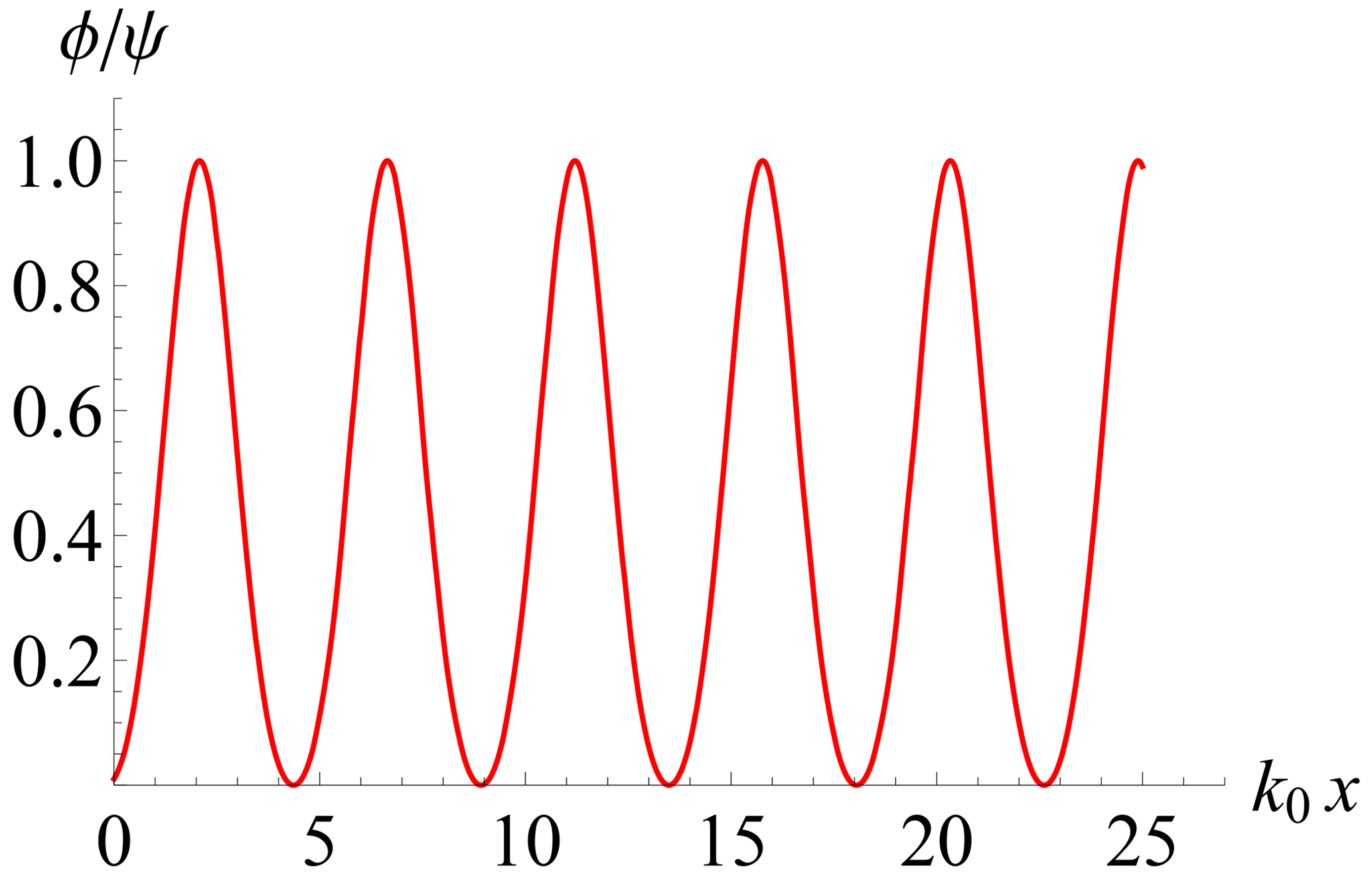
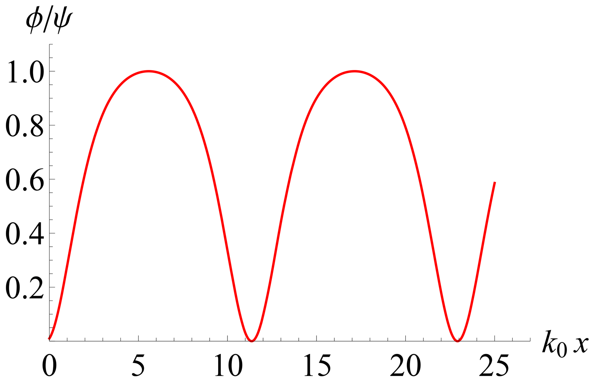
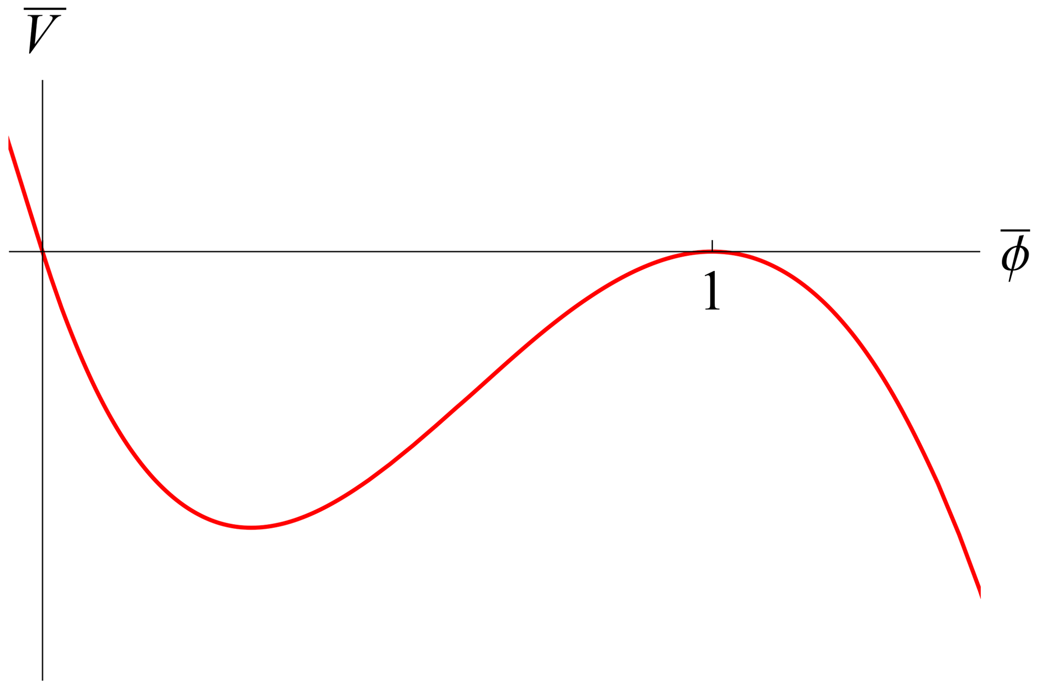
contains only one free parameter, $\stackrel{\mathrm{‾}}{b}$. Property (II) before Eq. (24) for periodic or localized solutions amounts to $\stackrel{\mathrm{‾}}{V}\left(\stackrel{\mathrm{‾}}{\mathit{\varphi }}\right)<\mathrm{0}$ within the interval $\mathrm{0}<\stackrel{\mathrm{‾}}{\mathit{\varphi }}<\mathrm{1}$. In view of the factorization in Eq. (31), it is easy to demonstrate that the condition is always satisfied for $\stackrel{\mathrm{‾}}{b}<\mathrm{1}$. The existence of periodic solutions such that $\mathrm{0}\le \stackrel{\mathrm{‾}}{\mathit{\varphi }}\le \mathrm{1}$ for $\stackrel{\mathrm{‾}}{b}<\mathrm{1}$ comes from the shape of the rescaled pseudopotential shown in Figs. 2 and 3. The case $\stackrel{\mathrm{‾}}{b}>\mathrm{1}$ also has periodic solutions but with a smaller amplitude, as is apparent from Fig. 4. The physically meaningful solutions always occur for $\stackrel{\mathrm{‾}}{V}<\mathrm{0}$ within the interval $\mathrm{0}<\stackrel{\mathrm{‾}}{\mathit{\varphi }}<\mathrm{1}$. Note that, with the further rescaling in Eq. (29), the amplitude of oscillation is set to unity, as shown in the referred figures. The required weakly nonlinear analysis always supposes that $\stackrel{\mathrm{̃}}{\mathit{\varphi }}\sim \mathrm{\Psi }\ll \mathrm{1}$ or, according to Eq. (13), $e\mathit{\varphi }/\left(m{\mathit{\theta }}^{\mathrm{2}}\right)\ll \mathrm{1}$, where ϕ is the physical scalar potential.

Figure 2 Rescaled pseudopotential from Eq. (31) for $\mathrm{0}<\stackrel{\mathrm{‾}}{b}<\mathrm{1}$.

Figure 3 Rescaled pseudopotential from Eq. (31) for $\stackrel{\mathrm{‾}}{b}\le \mathrm{0}$.

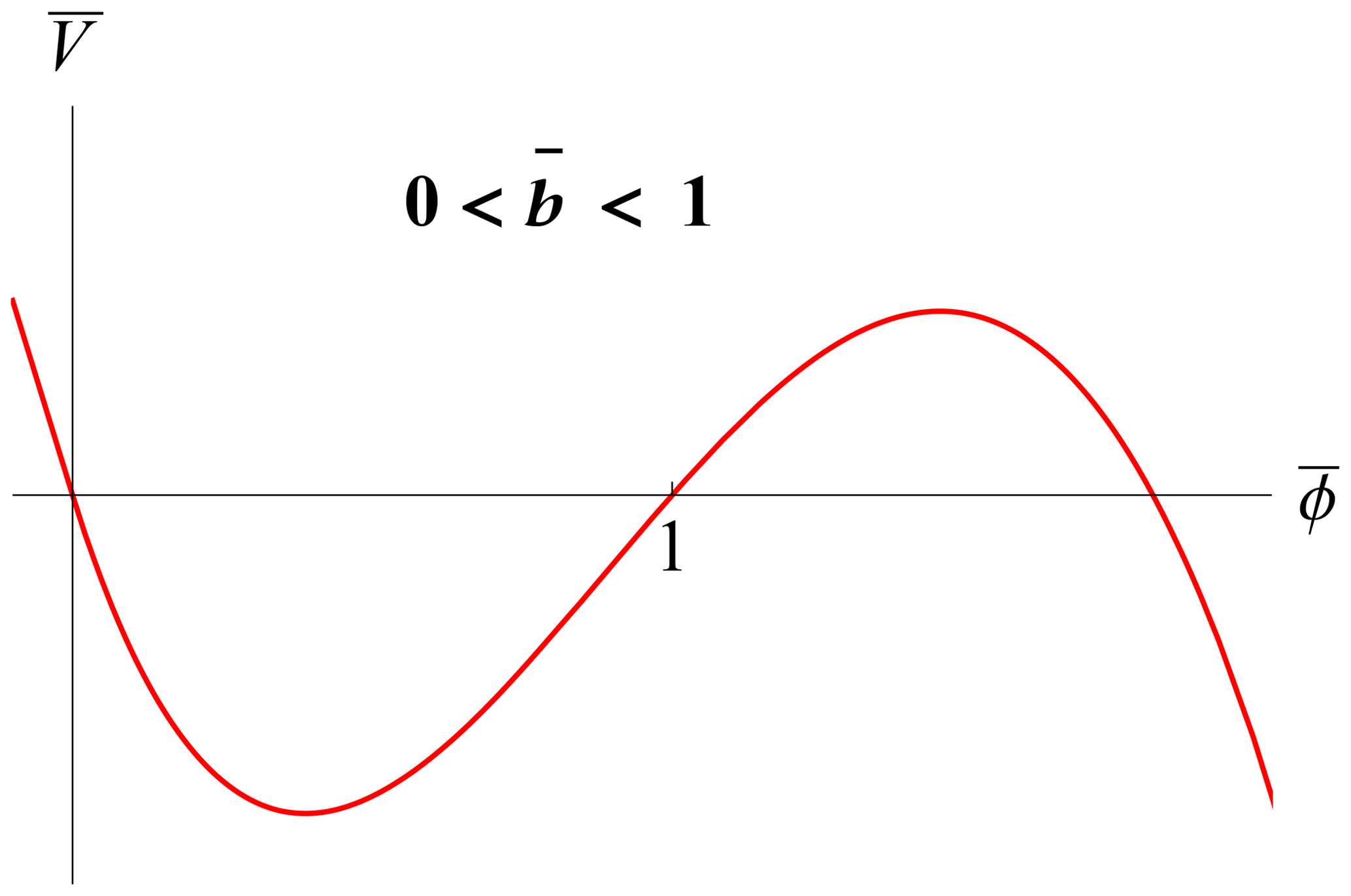
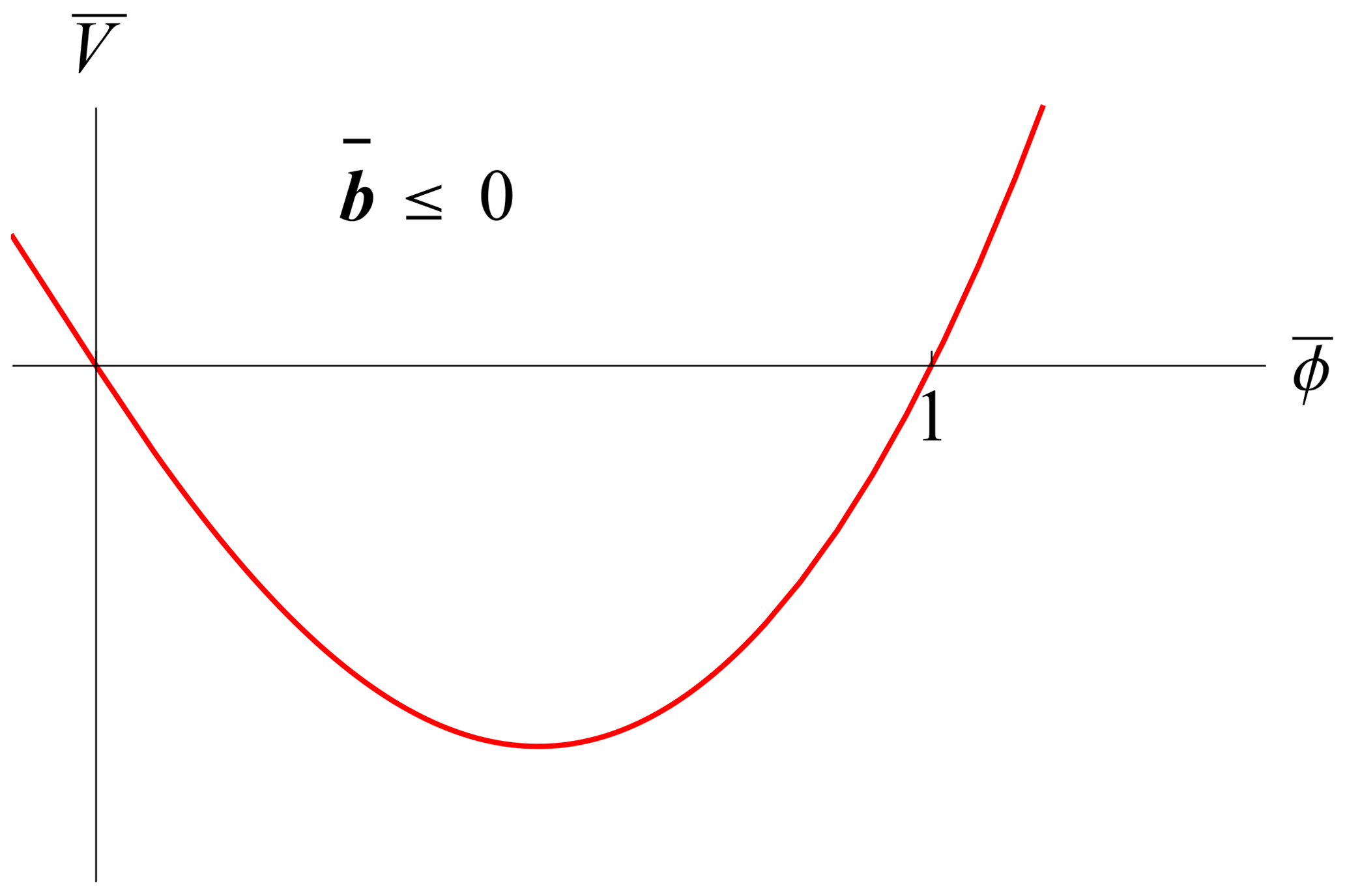
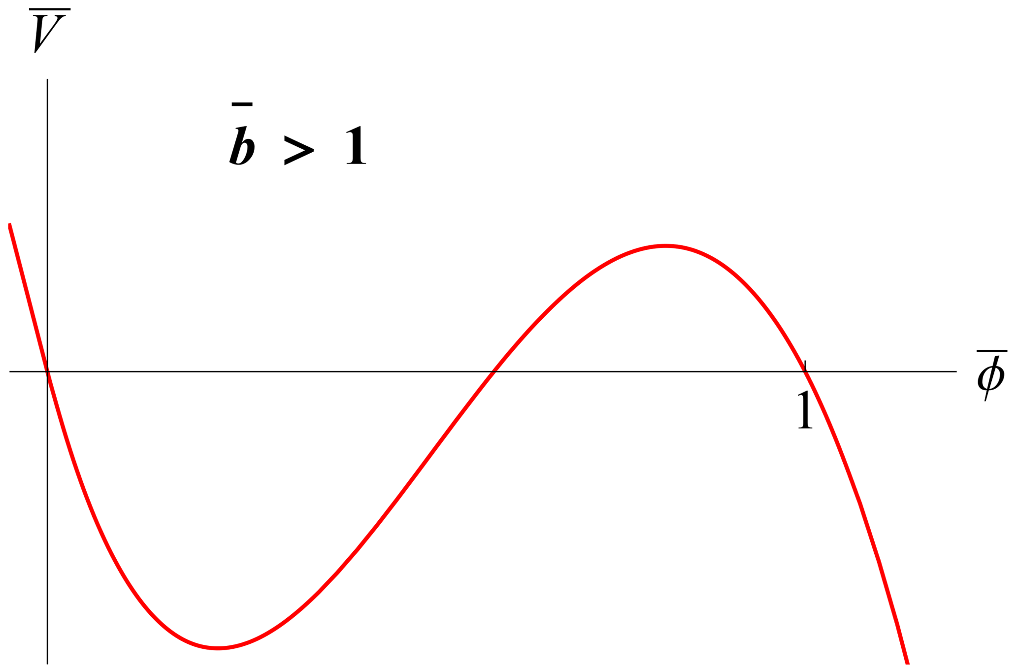
Figure 4 Rescaled pseudopotential from Eq. (31) for $\stackrel{\mathrm{‾}}{b}>\mathrm{1}$. Periodic solutions exist in a smaller interval: $\mathrm{0}\le \stackrel{\mathrm{‾}}{\mathit{\varphi }}<\mathrm{1}$.

The exact quadrature of Eq. (30) with all the terms was fully discussed in Schamel (2012, 2000), where the pseudopotential is formally the same as in Eq. (31) after rescaling. It is given in terms of Jacobi elliptic functions showing a periodic behavior and higher-order Fourier harmonics. The present work extends these results for the case of a background RKD with the adapted coefficients.

It is apparent that the control parameter $\stackrel{\mathrm{‾}}{b}$ depending on several variables such as the effective trapped particles' inverse temperature β determines the qualitative aspects of the oscillatory solutions. Figures 5–7 show in a different way how a smaller (and possibly negative) $\stackrel{\mathrm{‾}}{b}<\mathrm{1}$ corresponds to a larger wavenumber, which is exactly k₀, only in the linear case.

Figure 5 Numerical solution of Eq. (30) with $\stackrel{\mathrm{‾}}{b}=-\mathrm{2},\stackrel{\mathrm{‾}}{\mathit{\varphi }}\left(\mathrm{0}\right)={\mathrm{10}}^{-\mathrm{3}}$.

Figure 6 Numerical solution of Eq. (30) with $\stackrel{\mathrm{‾}}{b}=\mathrm{0.5},\stackrel{\mathrm{‾}}{\mathit{\varphi }}\left(\mathrm{0}\right)={\mathrm{10}}^{-\mathrm{3}}$.

Figure 7 Numerical solution of Eq. (30) with $\stackrel{\mathrm{‾}}{b}=\mathrm{0.9},\stackrel{\mathrm{‾}}{\mathit{\varphi }}\left(\mathrm{0}\right)={\mathrm{10}}^{-\mathrm{3}}$.

5.2 Localized solution with $\stackrel{\mathrm{‾}}{b}=\mathrm{1},k_{\mathrm{0}}\ne \mathrm{0}$

The limit case $\stackrel{\mathrm{‾}}{b}=\mathrm{1}$ with k₀≠0 is special, since then $\mathrm{d}\stackrel{\mathrm{‾}}{V}/\mathrm{d}\stackrel{\mathrm{‾}}{\mathit{\varphi }}=\mathrm{0}$ at $\stackrel{\mathrm{‾}}{\mathit{\varphi }}=\mathrm{1}$, as shown in Fig. 8, yielding a localized, non-periodic solution. Moreover, this case is amenable to the simple quadrature

$$\begin{array}{}\text{(32)}& \stackrel{\mathrm{‾}}{\mathit{\varphi }}={\displaystyle \frac{\mathrm{1}}{\mathrm{4}}}{\left[\mathrm{1}-\mathrm{3}{\tanh }^{\mathrm{2}}\left({\displaystyle \frac{\sqrt{\mathrm{3}}}{\mathrm{4}}}(\stackrel{\mathrm{‾}}{x}-{\stackrel{\mathrm{‾}}{x}}_{\mathrm{0}})\right)\right]}^{\mathrm{2}}\end{array}$$

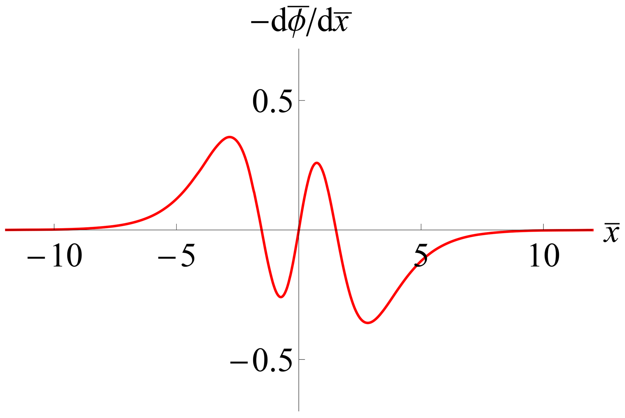
(see Fig. 9). The corresponding rescaled electric field is shown in Fig. 10. The total electrostatic energy is finite since the integral $(\mathrm{1}/\mathrm{2}){\int }_{-\mathrm{\infty }}^{\mathrm{\infty }}\mathrm{d}\stackrel{\mathrm{‾}}{x}(\mathrm{d}\stackrel{\mathrm{‾}}{\mathit{\varphi }}/\mathrm{d}\stackrel{\mathrm{‾}}{x}{)}^{\mathrm{2}}=\mathrm{6}\sqrt{\mathrm{3}}/\mathrm{35}$ converges.

Figure 8 Rescaled pseudopotential from Eq. (31) for $\stackrel{\mathrm{‾}}{b}=\mathrm{1}$.

Figure 9 Rescaled electrostatic potential from Eq. (32) for ${\stackrel{\mathrm{‾}}{x}}_{\mathrm{0}}=\mathrm{0}$.

Figure 10 Rescaled electric field $-\mathrm{d}\stackrel{\mathrm{‾}}{\mathit{\varphi }}/\mathrm{d}\stackrel{\mathrm{‾}}{x}$, where $\stackrel{\mathrm{‾}}{\mathit{\varphi }}$ is given in Eq. (32) for ${\stackrel{\mathrm{‾}}{x}}_{\mathrm{0}}=\mathrm{0}$.

5.3 Solitary waves with k₀=0

On the other hand, if k₀=0, one has

$$\begin{array}{}\text{(33)}& V={\displaystyle \frac{\mathrm{2}b{\mathit{\varphi }}^{\mathrm{2}}}{\mathrm{5}}}(\sqrt{\mathrm{\Psi }}-\sqrt{\mathit{\varphi }}),\end{array}$$

yielding the solitary pulse

$$\begin{array}{}\text{(34)}& \mathit{\varphi }=\mathrm{\Psi }{\text{sech}}^{\mathrm{4}}\left[{\left({\displaystyle \frac{-b\sqrt{\mathrm{\Psi }}}{\mathrm{20}}}\right)}^{\mathrm{1}/\mathrm{2}}(x-x_{\mathrm{0}})\right],\end{array}$$

which is well-defined everywhere provided that b<0, which can be attainable, e.g., for sufficiently small $\mathit{\beta },v_{\mathrm{0}}^{\mathrm{2}}$.

6 Dispersion relation

The NDR (24) provides several behaviors according to the values in the parameter space. For the sake of simplicity, this will be considered the case where the trapped particle distribution is homogeneous in phase space, which amounts to the dimensionless quantity β=0 in Eq. (10). This is an increasingly better approximation for small enough amplitudes so that eΨ≪mθ², yielding a relatively smaller trapped area in phase space. Clearly this limit situation does not correspond to “holes”, since in this case the trapped particles are not in a depression in phase space, as shown, e.g., in Fig. 1. However, the analytic simplicity motivates the approach. Furthermore, subcases can be identified: drifting, non-drifting, oscillating and non-oscillating as follows. Our main purpose is to provide an investigation showing regular behavior for small κ values as long as α>0.

6.1 Non-drifting, non-oscillating

If the trapped distribution is homogeneous and non-drifting with respect to the fixed ionic background (v₀=0), one has, from Eq. (24),

$$\begin{array}{}\text{(35)}& \begin{array}{rl}{k}_{\mathrm{0}}^{\mathrm{2}}& +{\displaystyle \frac{\mathrm{2}U\left(\frac{\mathrm{1}}{\mathrm{2}},\frac{\mathrm{1}}{\mathrm{2}}-\mathit{\kappa },{\mathit{\alpha }}^{\mathrm{2}}\mathit{\kappa }\right)}{\mathit{\kappa }U\left(\frac{\mathrm{3}}{\mathrm{2}},\frac{\mathrm{3}}{\mathrm{2}}-\mathit{\kappa },{\mathit{\alpha }}^{\mathrm{2}}\mathit{\kappa }\right)}}\\ & -{\displaystyle \frac{\mathrm{32}\sqrt{\mathrm{2}\mathrm{\Psi }}}{\mathrm{15}\mathit{\kappa }\sqrt{\mathit{\pi }\mathit{\kappa }}U\left(\frac{\mathrm{3}}{\mathrm{2}},\frac{\mathrm{3}}{\mathrm{2}}-\mathit{\kappa },{\mathit{\alpha }}^{\mathrm{2}}\mathit{\kappa }\right)}}=\mathrm{0}.\end{array}\end{array}$$

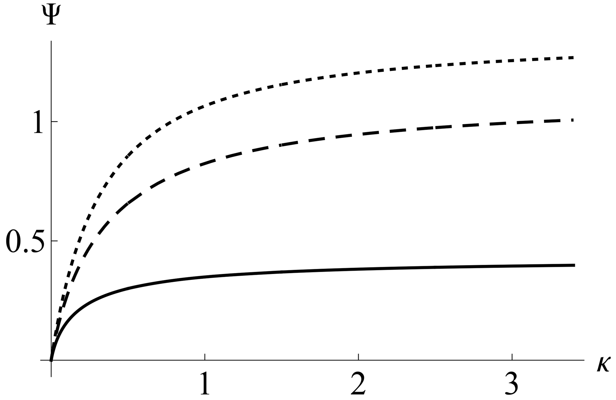
Figure 11 Solitary wave amplitude in the homogeneous trapped distribution, non-drifting and non-oscillating cases as a function of κ and different α from Eq. (36). Upper line, dotted: α=0.0; middle line, dashed: α=0.5; lower line, solid: α=1.5.

Furthermore, in the non-oscillating case k₀=0, one can solve Eq. (35) as

$$\begin{array}{}\text{(36)}& \mathrm{\Psi }={\displaystyle \frac{\mathit{\pi }}{\mathrm{2}}}\mathit{\kappa }{\left[{\displaystyle \frac{\mathrm{15}}{\mathrm{16}}}U\left({\displaystyle \frac{\mathrm{1}}{\mathrm{2}}},{\displaystyle \frac{\mathrm{1}}{\mathrm{2}}}-\mathit{\kappa },{\mathit{\alpha }}^{\mathrm{2}}\mathit{\kappa }\right)\right]}^{\mathrm{2}},\end{array}$$

which is the amplitude of the solitary wave in terms of the remaining parameters κ,α only. Figure 11 shows the resulting amplitude. The regular behavior as κ→0 is apparent. A larger α implies a smaller solitary wave amplitude. In the non-regularized limit α→0 it is possible to show that from Eq. (36) one has Ψ→1.38 as κ→∞, which is beyond the weakly nonlinear assumption. From Fig. 11 one also finds that the α=0 case only admits small-amplitude holes for κ≪1, which contradicts the constraint $\mathit{\kappa }>\mathrm{3}/\mathrm{2}$ for the non-regularized equilibrium. It is interesting to note that the weakly nonlinear condition Ψ≪1 is much better fulfilled for a sufficiently high α. Hence, such hole structures (with β=0, non-drifting and non-oscillating) are more reliable in an RKD background. Note, however, that high α values limit the extent of the power laws.

Figure 12 Wave amplitude in the homogeneous trapped distribution, non-drifting and oscillating cases as a function of κ and different wavenumbers for α=1.5 from Eq. (35). Lower line, solid: k₀=1.0; middle line, dashed: k₀=1.5; upper line, dotted: k₀=2.0.

6.2 Non-drifting, oscillating

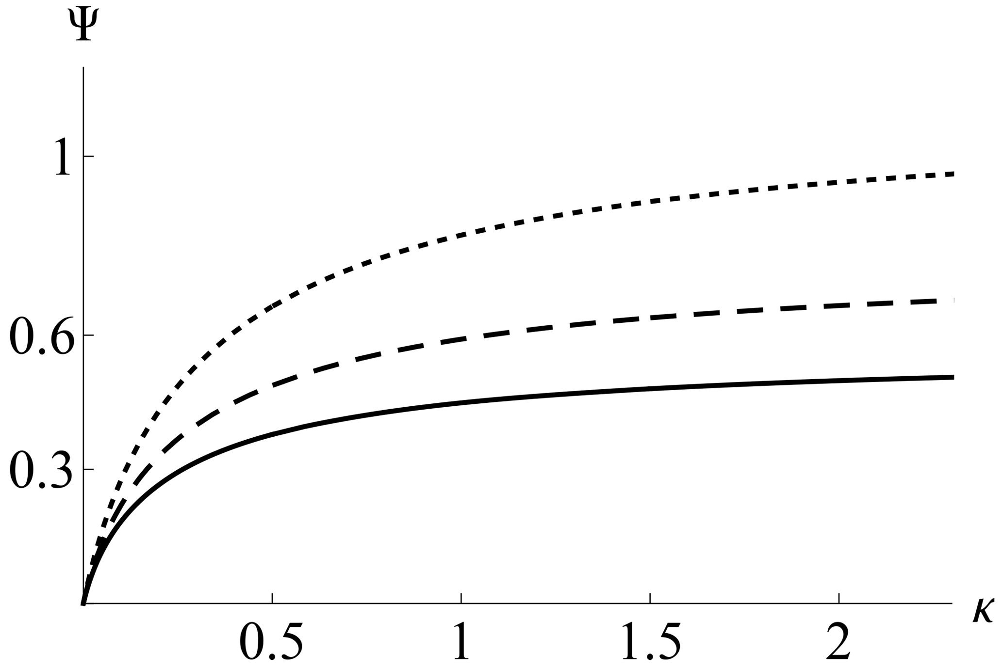
Allowing k₀≠0 for oscillating solutions, one also has a regular behavior of the amplitude as κ≪1. In this limit, assuming α>0, it can be shown that Eq. (35) reduces to

$$\begin{array}{}\text{(37)}& k_{\mathrm{0}}^{\mathrm{2}}+{\displaystyle \frac{\sqrt{\mathit{\pi }}\mathit{\alpha }}{\sqrt{\mathit{\kappa }}}}-{\displaystyle \frac{\mathrm{32}\mathit{\alpha }\sqrt{\mathrm{\Psi }}}{\mathrm{15}\sqrt{\mathrm{2}\mathit{\pi }}\mathit{\kappa }}}=\mathrm{0},\mathit{\kappa }\ll \mathrm{1},\mathit{\alpha }>\mathrm{0},\end{array}$$

yielding a vanishingly small amplitude as κ→0. Figure 12 shows Ψ from Eq. (35) as a function of κ for α=1.5 and different k₀ values. It is found that a larger k₀ yields a larger amplitude.

6.3 Dispersion relation with v₀≠0

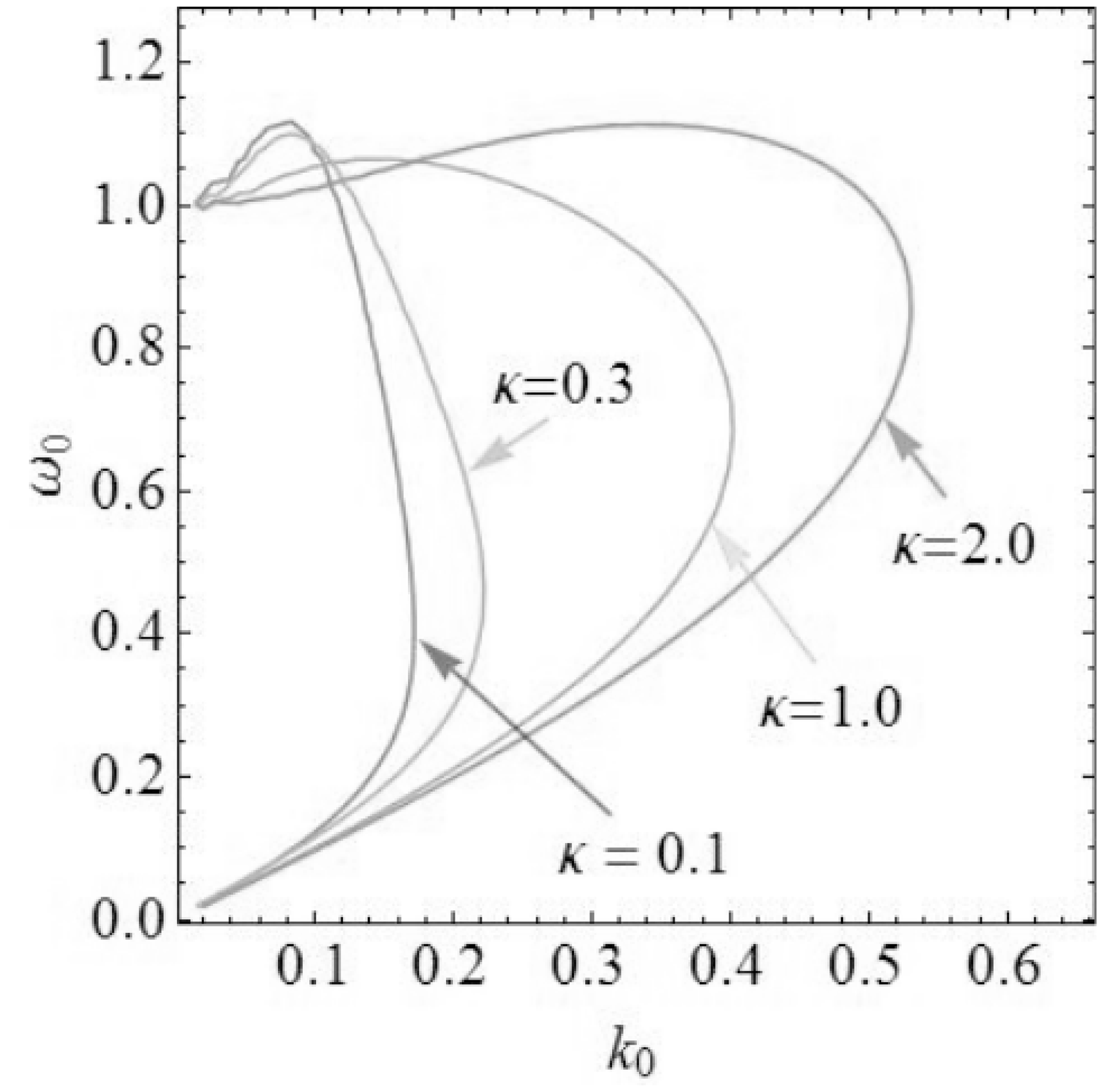
Allowing for drifting structures so that v₀≠0, for simplicity, disregarding the nonlinear term $\sim b\sqrt{\mathrm{\Psi }}$ and still with a homogeneous trapped electron distribution (β=0), one has, from Eq. (24),

$$\begin{array}{}\text{(38)}& \begin{array}{rl}{k}_{\mathrm{0}}^{\mathrm{2}}& +{\displaystyle \frac{\mathrm{2}}{\mathit{\kappa }U\left(\frac{\mathrm{3}}{\mathrm{2}},\frac{\mathrm{3}}{\mathrm{2}}-\mathit{\kappa },{\mathit{\alpha }}^{\mathrm{2}}\mathit{\kappa }\right)}}[U\left({\displaystyle \frac{\mathrm{1}}{\mathrm{2}}},{\displaystyle \frac{\mathrm{1}}{\mathrm{2}}}-\mathit{\kappa },{\mathit{\alpha }}^{\mathrm{2}}\mathit{\kappa }\right)\\ & +{\displaystyle \frac{v_{\mathrm{0}}}{\sqrt{\mathit{\pi }\mathit{\kappa }}}}P\underset{-\mathrm{\infty }}{\overset{\mathrm{\infty }}{\int }}{\displaystyle \frac{\mathrm{d}s}{s-v_{\mathrm{0}}}}{e}^{-{\mathit{\alpha }}^{\mathrm{2}}{s}^{\mathrm{2}}}{\left(\mathrm{1}+{\displaystyle \frac{s^{\mathrm{2}}}{\mathit{\kappa }}}\right)}^{-\mathit{\kappa }-\mathrm{1}}]=\mathrm{0}.\end{array}\end{array}$$

Setting $v_{\mathrm{0}}={\mathit{\omega }}_{\mathrm{0}}/k_{\mathrm{0}}$, Eq. (38) produces similar thumb curves to holes in a Maxwellian background (Schamel, 1986), now adapted for the RKD. Figure 13 shows results for different small κ values, in all cases with α=0.1. As usual, one has a high-frequency (Langmuir) mode together with a slow electron-acoustic mode (Fried, 1961) now adapted to the RKD background, where both modes coalesce at a certain point according to the parameters. As seen, the behavior is regular even for small κ values. At the extremal k value where both modes coalesce, apparently the group velocity is infinite. As discussed in Schamel (2013) and Valentini (2012), at this point taking into account the nonlinear trapping, the phase velocity of the hole should replace the diverging linear group velocity.

Figure 13 Dispersion relation (38) with $v_{\mathrm{0}}={\mathit{\omega }}_{\mathrm{0}}/k_{\mathrm{0}}$ for α=0.1 and $\mathit{\kappa }=\mathrm{0.1},\mathrm{0.3},\mathrm{1.0}$ and 2.0, as indicated.

7 Conclusions

In the present paper, electron holes have been discussed for the first time in a suprathermal plasma described with a regularized kappa distribution. Unlike Haas (2021), for simplicity, here the background distribution function has no singular features. It was verified that the regularization of the standard kappa distribution avoids all divergent features of the solutions for $\mathit{\kappa }\le \mathrm{3}/\mathrm{2}$; i.e., the analysis could be extended to all positive kappa values. This allows one to study plasma backgrounds that are described with velocity power laws harder than v⁻⁵ and those that exhibit an exponential cutoff, which are both observed in the solar wind. Note also that, even for kappa values below 2, which can technically be handled with an SKD, unphysical features related to a non-negligible contribution of particles at high velocities are unavoidable (Scherer, 2019). Their removal also requires the use of an RKD.

In terms of the hole distribution function for trapped and untrapped electrons, the number density has been evaluated, yielding the pseudopotential in the weakly nonlinear limit. As a consequence, the most prominent solutions of the resulting Poisson equation have been found. Drifting, non-drifting, oscillating and non-oscillating solutions have been discussed. The linear dispersion relation has also been analyzed, yielding a κ-dependent plasma-mode diagram revealing the existence of a high-frequency Langmuir mode and a low-frequency electron acoustic mode (Fig. 13). Unlike for the case of a pure power law, i.e., for an SKD background, all findings based on power laws with an exponential cutoff, i.e., based on an RKD background, remain regular even for very small κ values. The results are, therefore, relevant especially for those plasmas in a suprathermal equilibrium state with a spectral index $\mathit{\kappa }<\mathrm{3}/\mathrm{2}$ for which the SKD is not appropriate but which is observed in space plasmas (Gloeckler et al., 2012).