Review article: Large fluctuations in non-equilibrium physics

Non-equilibrium is dominant in geophysical and climate phenomena. However the study of non-equilibrium is much more difficult than equilibrium, and the relevance of probabilistic simplified models has been emphasized. Large deviation rates have been used recently in climate science. In this paper, after recalling progress during the last decades in understanding the role of large deviations in a class of non-equilibrium systems, we point out differences between equilibrium and non-equilibrium. For example, in non-equilibrium (a) large deviation rates may be extensive but not simply additive. (b) In non-equilibrium there are generically long-range space correlations, so large deviation rates are non-local. (c) Singularities in large deviation rates denote the existence of phase transitions often not possible in equilibrium. To exemplify, we shall refer to lattice gas models like the symmetric simple exclusion process and other models which are playing an important role in the understanding of non-equilibrium physics. The reasons why all this may be of interest in climate physics will be briefly indicated.

1 Introduction

This paper is an enlarged version of a seminar in the series Perspectives in Climate Sciences 2021 and provides an introduction to the main ideas of the so-called macroscopic fluctuation theory (MFT). This theory developed mainly for non-equilibrium diffusive systems is very well supported by mathematical models and provides a methodological approach that can be followed for other non-equilibrium systems.

The theory is based on variational principles determining for each model the large deviation rates (LDRs) of thermodynamic variables like a density or a time average like the time-averaged current flowing through the system in stationary states. Models in climate science are considerably more complex than those for which MFT has been proved to hold. However, MFT may provide a guide for more complex problems, and it shows that there are considerable differences in fluctuations from an equilibrium or a non-equilibrium state.

In the last decades, the theory of large deviations has become a main tool in statistical mechanics especially in the study of non-equilibrium. MFT has been formulated and verified in probabilistic models of lattice gases which macroscopically lead to hydrodynamic diffusion equations, which in turn represent laws of large numbers. Therefore, large deviations from hydrodynamic behavior have been studied. Here, we shall follow the formulation given in Bertini et al. (2001, 2002) and the reviews in Bertini et al. (2007, 2015). The reader is advised to refer also to Derrida (2007, 2011). Although the theory has been developed especially for diffusions, several conclusions seem to hold more generally, e.g., for reaction–diffusion systems (Jona-Lasinio et al., 1993). Reaction–diffusion systems include important energy balance models in geophysics (Sellers, 1969; Ghil, 1976).

Non-equilibrium is dominant in geophysical and climate phenomena, and we refer to the following papers for the relevance of large deviation estimates in this domain (Galfi et al., 2019; Galfi and Lucarini, 2021; Galfi et al., 2021); see also Lucarini et al. (2022). In Galfi et al. (2019), a simplified model of the general circulation of the atmosphere is adopted and assumed to be a chaotic dynamical system so that probabilistic concepts and methods can be applied. Stochastic climate models were introduced by Hasselmann (1976). For a recent assessment of the Hasselmann program, we refer to Lucarini and Chekroun (2023).

Non-equilibrium includes an enormous variety of phenomena, so we cannot hope to formulate a unique theory having a generality comparable to classical thermodynamics. We have to restrict to subclasses of problems. One difficulty is to define suitable thermodynamic functionals in far from equilibrium situations. Large fluctuations have offered a way out, as large deviation rates provide genuine thermodynamic functionals in non-equilibrium stationary states.

Studying irreversible processes is much more difficult than understanding equilibrium phenomena. In equilibrium statistical mechanics, we do not have to solve any equation of motion, and the Gibbs distribution provides the basis for the calculation of macroscopic quantities and their fluctuations. In non-equilibrium, we cannot bypass the dynamics even in the study of stationary states, which we may consider as the simplest beyond equilibrium. Examples are the heat flow in an iron rod whose endpoints are thermostated at different temperatures or the stationary flow of electrical current in a given potential difference.

For such states, the fluctuations exhibit novel and rich features with respect to the equilibrium situation. As experimentally observed (Dorfman et al., 1994), the space correlations of the thermodynamic variables generically extend to macroscopic distances, which means, for instance, that the fluctuations of the density in different points of the system are not independent. This is reflected in the structure of large deviation rates, which in non-equilibrium stationary states are in general non-local in space.

In this paper, we consider a class of systems that behave macroscopically as diffusions. The systems considered locally deviate only slightly from equilibrium so that small gradients and linear response to external fields are reasonable approximations. Microscopically, this implies that the system reaches a local equilibrium in a time which is short compared to the times typical of macroscopic evolution. So what characterizes situations in which this description applies is a separation of scales both in space and time. Far from equilibrium states are those which exhibit differences over the size of the whole system. In other words, far from equilibrium is obtained from building up small local differences. Local equilibrium is the first assumption we make. For the relevance of local equilibrium in climate models, see Lorenz (1967), Peixoto and Oort (1992).

This restriction allows us to understand some typical phenomena induced by non-equilibrium in somewhat ideal cases which however give a hint of what may happen in more realistic cases.

The content of the paper is as follows: in the next section, we recall the use by Einstein of the Boltzmann relation between entropy and probability to estimate the probability of a thermodynamic fluctuation in equilibrium. In Sect. 3, we describe the essentials of the macroscopic fluctuation theory in the version reviewed in Bertini et al. (2015). Section 4 is devoted to the illustration of the differences between equilibrium and non-equilibrium through explicit calculations for the symmetric simple exclusion process (SSEP). Final comments are in Sect. 5. Our exposition is not very detailed, and if the reader wants to understand the underpinning calculations, we suggest consulting the reviews by Bertini et al. (2015), Derrida (2007, 2011), Mallick (2015) and references therein.

2 Macroscopic fluctuations in equilibrium

The first explicit large deviation theory in equilibrium states is presumably Einstein's theory of opalescence (Einstein, 1910); see also Landau and Lifshitz (1980). He uses the Boltzmann–Planck formula connecting entropy and probability to estimate probabilities of fluctuations of thermodynamic variables, e.g., of densities. Therefore, entropy appears as a large deviation rate. The small parameter representing the intensity of the noise in this case is the Boltzmann constant (Bertini et al., 2015), $\mathit{\kappa }=R/N$, R is the gas constant, and N is Avogadro's number, so that its inverse is proportional to the typical number of the microscopic degrees of freedom of the system. Einstein's paper, which is entirely correct far from the critical point, unfortunately contains an improper application to the critical point where long-range correlations are present. This paper was criticized later by Ornstein and Zernike (1914) but provided an important source of inspiration for non-equilibrium.

Starting from what he calls the Boltzmann principle,

$$\begin{array}{}\text{(1)}& S=\mathit{\kappa }\ln W+\text{const},\end{array}$$

it is interesting to quote from Einstein (1910) the following:

W is commonly equated with the number of different possible ways (complexions) in which the state considered – which is incompletely defined in the sense of a molecular theory, by parameters of a system – can conceivably be realized. To be able to calculate W, one needs a complete theory of the system under consideration. If considered from a phenomenological point of view Eq. (1) appears devoid of content.

However, Boltzmann's principle does acquire some content independent of any elementary theory if one assumes and generalizes from molecular kinetics the proposition that the irreversibility of physical processes is only apparent.

It follows from Eq. (1) that

$$\begin{array}{}\text{(2)}& W=\text{const}\cdot e^{\frac{N}{R}S}.\end{array}$$

The order of magnitude of the constant is determined by taking into account that for the state of maximum entropy (entropy S₀), W is of the order of magnitude 1, so that we then have, with order of magnitude accuracy,

$$\begin{array}{}\text{(3)}& W=e^{\frac{N}{R}(S-S_{\mathrm{0}})}.\end{array}$$

From this, we can conclude that the probability dW that the quantities λ₁….λ_k lie between λ₁ and λ₁+dλ₁......λ_k, and λ_k+dλ_k is given, in order of magnitude, by the equation

$$\begin{array}{}\text{(4)}& \mathrm{d}W=e^{\frac{N}{R}(S-S_{\mathrm{0}})}\mathrm{d}{\mathit{\lambda }}_{\mathrm{1}}\mathrm{\dots }\mathrm{d}{\mathit{\lambda }}_k,\end{array}$$

in the case when the system is determined only incompletely by λ₁….λ_k.

In 1931, Onsager (1931a, b), in the same vein as Einstein (1910) that was quoted, made use of the Boltzmann formula in the study of fluctuations in non-equilibrium phenomena under the condition of small global deviations from equilibrium. The theory was developed further by Onsager and Machlup in Onsager and Machlup (1953) where fluctuations of time trajectories of thermodynamic variables were considered under the same hypotheses. In the next section, we discuss how it is possible to give a meaning to a formula like Eq. (3) in the more general situation of stationary states non-necessarily close to equilibrium. Typically we think of systems in contact with thermostats at different temperatures and/or reservoirs characterized by different chemical potentials and under the action of external fields. The MFT represents a step forward with respect to Onsager and the Onsager–Machlup theory.

To study the fluctuations in states far from equilibrium, let us analyze the meaning of the difference S−S₀ in Eq. (3). In an isolated system, energy is conserved so that, if the volume remains constant, $S-S_{\mathrm{0}}=-\frac{F-F_{\mathrm{0}}}{T}$ where F is the Helmholtz free energy. The quantity F₀−F, it represents the minimal work to bring the equilibrium state to the state corresponding to F at constant temperature and volume (Landau and Lifshitz, 1980) where F₀ is the equilibrium free energy different for different systems.

The concept of minimal work is meaningful also in non-equilibrium and can be taken as a generalization of the free energy. This is essentially the starting point of the macroscopic fluctuation theory. In the following section, we shall present the basic ideas of the MFT, stating explicitly the main assumptions, following mainly Bertini et al. (2015).

3 Macroscopic fluctuation theory (MFT)

The MFT, as we mentioned, was inspired by non-equilibrium microscopic probabilistic models, or the so-called lattice gases, in particular the symmetric simple exclusion process (SSEP) for which the macroscopic dynamics are diffusive and can be proved rigorously. Also the probabilities of large deviations can be obtained and the rates computed. For a general introduction to lattice gases, we refer to Spohn (1991).

3.1 Macroscopic fluctuations in stationary states

The macroscopic dynamics of diffusive systems are described by hydrodynamic equations often provided by conservation laws and constitutive equations; that is equations expressing the current in terms of the thermodynamic variables. More precisely on the basis of a local equilibrium assumption, at the macroscopic level, the system is completely described by a local density ρ(t,x), which may have several components and the local current j(t,x). The evolution equations are of the form

$$\begin{array}{}\text{(5)}& \left\{\begin{array}{l}{\partial }_t\mathit{\rho }\left(t\right)+\mathrm{\nabla }\cdot j\left(t\right)=\mathrm{0},\\ j\left(t\right)=J(t,\mathit{\rho }(t\left)\right),\end{array}\right.\end{array}$$

where we omit the space variable $x\in \mathrm{\Lambda }\subset R^d$.

For diffusive systems, the constitutive equations take the following form:

$$\begin{array}{}\text{(6)}& J\left(\mathit{\rho }\right)=-D\left(\mathit{\rho }\right)\mathrm{\nabla }\mathit{\rho }+\mathit{\chi }\left(\mathit{\rho }\right)E,\end{array}$$

where the diffusion coefficient D(ρ) and the mobility χ(ρ) are d×d symmetric and positive definite matrices, and E is an external field acting on the bulk.

These equations have to be supplemented by appropriate boundary conditions on ∂Λ, the boundary of Λ. If λ(t,x), $x\in \partial \mathrm{\Lambda }$ is the chemical potential of the external reservoirs, the boundary conditions read

$$\begin{array}{}\text{(7)}& f^{\prime }\left(\mathit{\rho }\right(t,x\left)\right)=\mathit{\lambda }(t,x),x\in \partial \mathrm{\Lambda },\end{array}$$

where f(ρ) is the equilibrium free energy density. Non-equilibrium depends on the boundary conditions and the external field. It may happen that the two equilibrate each other, in which case we have a non-homogeneous equilibrium state. Much of what we shall say applies to equations which are not in divergence form.

We assume that the microscopic evolution is given by a Markov process X_t which represents the configuration of the system at time t. The stationary non-equilibrium state (SNS) is described by a stationary, i.e., invariant with respect to time shifts, probability distribution P_st over the trajectories of X_t.

The macroscopic equations are supposed to derive from an underlying microscopic dynamics through an appropriate scaling limit where the microscopic time is divided by a factor ≈N² and space is divided by ≈N for N tending to ∞ where N is the number of degrees of freedom of the system.

The hydrodynamic equations represent laws of large numbers with respect to the probability measure P_st conditioned on an initial state X₀. The initial conditions are determined by X₀. Of course many microscopic configurations give rise to the same value of ρ₀(x). In general ρ_t(x) is an appropriate limit as the number of degrees of freedom diverges.

Classically we should start from molecules interacting with realistic forces and evolving with Newtonian dynamics. This is beyond the reach of present-day mathematical theory, and much simpler models have to be adopted in the reasonable hope that some essential features are adequately captured.

We further assume that the stationary measure P_st admits a principle of large deviations describing the fluctuations from the typical hydrodynamic behavior. This means that the probability that the macroscopic variable ρ_t deviates from the solutions of the hydrodynamic equations and is close to some trajectory ${\widehat{\mathit{\rho }}}_t$ is exponentially small and of the following form:

$$\begin{array}{}\text{(8)}& \begin{array}{rl}{P}_{\mathrm{st}}\left(\mathit{\rho }\left(X_t\right)\approx {\widehat{\mathit{\rho }}}_t\left(u\right),t\in [t_{\mathrm{1}},t_{\mathrm{2}}]\right)& \approx e^{-\frac{\mathrm{1}}{{\mathit{ϵ}}^d}\left[V\right({\widehat{\mathit{\rho }}}_{t_{\mathrm{1}}})+\mathcal{J}(\widehat{\mathit{\rho }}\left)\right]}\\ & =e^{-\frac{\mathrm{1}}{{\mathit{ϵ}}^d}I\left(\widehat{\mathit{\rho }}\right)},\end{array}\end{array}$$

where $\mathcal{J}\left(\widehat{\mathit{\rho }}\right)$ is a positive functional which vanishes if ${\widehat{\mathit{\rho }}}_t$ is a solution of Eq. (5), and $V\left({\widehat{\mathit{\rho }}}_{t_{\mathrm{1}}}\right)$ is the cost to produce the initial value ${\widehat{\mathit{\rho }}}_{t_{\mathrm{1}}}$. The parameter ϵ is a scaling factor of the order of the ratio between the microscopic length scale (typical intermolecular distance) and the macroscopic one. The factor ϵ^−d is of the order of the number of particles in a macroscopic volume. The role of Avogadro's number in Eq. (3) is played here by ϵ^d. We normalize $V\left(\widehat{\mathit{\rho }}\right)$ so that $V\left(\widehat{\mathit{\rho }}\right)=\mathrm{0}$ when $\widehat{\mathit{\rho }}=\overline{\mathit{\rho }}$ is the stationary solution. Therefore $\mathcal{J}\left(\widehat{\mathit{\rho }}\right)$ represents the extra cost necessary in order that the system follows the trajectory ${\widehat{\mathit{\rho }}}_t$. Finally $\mathit{\rho }\left(X_t\right)\approx {\widehat{\mathit{\rho }}}_t$ means closeness in some metric. V is the generalization to the infinite dimensional case of the Freidlin–Wentzell quasi-potential (Freidlin and Wentzell, 2012) and is the large deviation rate of the stationary probability measure. The exponent in Eq. (8) due to the factor ϵ^−d is extensive in space. When we consider large deviations of a time-averaged quantity like the current (Bertini et al., 2005b), we get an extra time factor.

Let us denote by θ the time inversion operator defined by $\mathit{\theta }{X}_t=X_{-t}=X_t^{*}$. The probability measure $P_{\mathrm{st}}^{*}$ describing the evolution of the time-reversed process $X_t^{*}$ is given by the composition of P_st and θ⁻¹ that is

$$\begin{array}{}\text{(9)}& P_{\mathrm{st}}^{*}(X_t^{*}={\mathit{\varphi }}_t,t\in [t_{\mathrm{1}},t_{\mathrm{2}}\left]\right)=P_{\mathrm{st}}(X_t={\mathit{\varphi }}_{-t},t\in [-t_{\mathrm{2}},-t_{\mathrm{1}}\left]\right).\end{array}$$

We assume that the time-reversed process also admits a hydrodynamic description. This hypothesis is physically very reasonable: by acting on a system from the outside, we can invert the currents flowing through the system and for example have heat passing from lower temperature to higher temperature.

At the level of large deviations, Eq. (9) implies

$$\begin{array}{}\text{(10)}& V\left({\widehat{\mathit{\rho }}}_{t_{\mathrm{1}}}\right)+{\mathcal{J}}_{[t_{\mathrm{1}},t_{\mathrm{2}}]}^{*}\left(\widehat{\mathit{\rho }}\right)=V\left({\widehat{\mathit{\rho }}}_{t_{\mathrm{2}}}\right)+{\mathcal{J}}_{[-t_{\mathrm{2}},-t_{\mathrm{1}}]}\left(\mathit{\theta }\widehat{\mathit{\rho }}\right),\end{array}$$

where ${\widehat{\mathit{\rho }}}_{t_{\mathrm{1}}}$, ${\widehat{\mathit{\rho }}}_{t_{\mathrm{2}}}$ represents the initial and final points of the trajectory and $V\left({\widehat{\mathit{\rho }}}_{t_i}\right)$ represents the costs associated with the creation of the fluctuations ${\widehat{\mathit{\rho }}}_{t_i}$ starting from the stationary non-equilibrium state (SNS). The functional 𝒥^* vanishes on the solutions of the hydrodynamics associated to the time-reversed process.

The physical situation we are considering is the following. The system is in the stationary state $\overline{\mathit{\rho }}$ at $t=-\mathrm{\infty }$, but at t=0 we find it in the state ${\widehat{\mathit{\rho }}}_{\mathrm{0}}$. We want to determine the most probable trajectory followed in the spontaneous creation of this fluctuation. According to Eq. (8), this trajectory is the one that minimizes 𝒥 among all trajectories connecting $\overline{\mathit{\rho }}$ to ${\widehat{\mathit{\rho }}}_{\mathrm{0}}$ in the time interval $[-\mathrm{\infty },\mathrm{0}]$. From Eq. (10) we have

$$\begin{array}{}\text{(11)}& {\mathcal{J}}_{[-\mathrm{\infty },\mathrm{0}]}\left(\widehat{\mathit{\rho }}\right)={\mathcal{J}}_{[\mathrm{0},\mathrm{\infty }]}^{*}\left(\mathit{\theta }\widehat{\mathit{\rho }}\right)+V\left({\widehat{\mathit{\rho }}}_{\mathrm{0}}\right).\end{array}$$

The right-hand side is minimal if ${\mathcal{J}}_{[\mathrm{0},\mathrm{\infty }]}^{*}\left(\mathit{\theta }\widehat{\mathit{\rho }}\right)=\mathrm{0}$; that is if $\mathit{\theta }\widehat{\mathit{\rho }}$ is a solution of the time-reversed hydrodynamics. The existence of such a relaxation solution is due to the fact that the stationary solution $\overline{\mathit{\rho }}$ is attractive also for the time-reversed hydrodynamics. We have therefore the following generalization of Onsager–Machlup to non-equilibrium stationary states:

In a SNS the spontaneous emergence of a macroscopic fluctuation takes place most likely following a trajectory which is the time reversal of the relaxation path according to the time-reversed hydrodynamics.

The above statement follows from assuming the existence of a time-reversed dynamics and from our general hypotheses. In equilibrium, a fluctuation emerges following the time reversal of the relaxation trajectory. As illustrated in Gabrielli et al. (1996, 1999), this property may hold even if the microscopic dynamics do not satisfy detailed balance. Therefore Onsager symmetry and the above non-equilibrium generalization can be true under rather general conditions: this is possible because going from the microscopic to the macroscopic level there is a loss of information.

From Eqs. (10) or (11) we have that the free energy is related to 𝒥 by

$$\begin{array}{}\text{(12)}& V\left(\mathit{\rho }\right)=\underset{\widehat{\mathit{\rho }}}{inf}{\mathcal{J}}_{[-\mathrm{\infty },\mathrm{0}]}\left(\widehat{\mathit{\rho }}\right),\end{array}$$

where the infimum is taken over all trajectories connecting $\overline{\mathit{\rho }}$ to ρ.

3.2 Density fluctuations

The functional 𝒥 for diffusive systems has the Freidlin–Wentzell form (Freidlin and Wentzell, 2012) generalized to the infinite dimensional situation.

$$\begin{array}{}\text{(13)}& \mathcal{J}={\displaystyle \frac{\mathrm{1}}{\mathrm{2}}}\int \mathrm{d}t\int \mathrm{d}x({\partial }_t\mathit{\rho }+\mathrm{\nabla }J(\mathit{\rho }\left)\right)K\left(\mathit{\rho }{)}^{-\mathrm{1}}\right({\partial }_t\mathit{\rho }+\mathrm{\nabla }J\left(\mathit{\rho }\right)),\end{array}$$

where the kernel K(ρ) is the elliptic operator defined on functions $\mathit{\pi }:\mathrm{\Lambda }\to \mathbf{R}$ vanishing at the boundary ∂Λ by

$$\begin{array}{}\text{(14)}& K\left(\mathit{\rho }\right)\mathit{\pi }=-\mathrm{\nabla }\cdot \left(\mathit{\chi }\right(\mathit{\rho }\left)\mathrm{\nabla }\mathit{\pi }\right).\end{array}$$

This operator is the generalization of the Onsager matrix. Interpreting $\mathcal{J}(\mathit{\rho },{\partial }_t\mathit{\rho })$ as a Lagrangian, there corresponds by Legendre duality the Hamiltonian

$$\begin{array}{}\text{(15)}& \mathcal{H}={\displaystyle \frac{\mathrm{1}}{\mathrm{2}}}\langle \mathrm{\nabla }H,\mathit{\chi }\left(\mathit{\rho }\right)\mathrm{\nabla }H\rangle +{\displaystyle \frac{\mathrm{1}}{\mathrm{2}}}\langle H,\mathrm{\nabla }\cdot \left(D\right(\mathit{\rho }\left)\mathrm{\nabla }\mathit{\rho }\right)\rangle ,\end{array}$$

where H is the momentum conjugate to ρ; that is $H=\frac{\mathit{\delta }\mathcal{L}}{\mathit{\delta }\left({\partial }_t\mathit{\rho }\right)}$. The scalar product 〈,〉 means integration over x.

The associated Hamilton equations are

$$\begin{array}{}\text{(16)}& \left\{\begin{array}{ll}{\partial }_t\mathit{\rho }& ={\displaystyle \frac{\mathit{\delta }\mathcal{H}}{\mathit{\delta }H}}={\displaystyle \frac{\mathrm{1}}{\mathrm{2}}}\mathrm{\nabla }\cdot \left(D\left(\mathit{\rho }\right)\mathrm{\nabla }\mathit{\rho }\right)-\mathrm{\nabla }\cdot \left(\mathit{\chi }\right(\mathit{\rho }\left)\mathrm{\nabla }H\right)\\ {\partial }_{t}H& ={\displaystyle }-{\displaystyle \frac{\mathit{\delta }\mathcal{H}}{\mathit{\delta }\mathit{\rho }}}\\ & ={\displaystyle }-{\displaystyle \frac{\mathrm{1}}{\mathrm{2}}}\sum _{\mathrm{1}\le i,j\le d}\left[{\mathit{\chi }}_{i,j}^{\prime }\left(\mathit{\rho }\right){\partial }_{x_i}H{\partial }_{x_j}H\right.\\ & \left.+D_{i,j}\left(\mathit{\rho }\right){\partial }_{x_i}{\partial }_{x_j}H\right].\end{array}\right.\end{array}$$

These equations with appropriate boundary conditions are the variational equations to calculate the optimal trajectory creating ρ. They characterize the MFT. They are difficult to solve for generic dependence on ρ of the transport coefficients D(ρ),χ(ρ). The variational problem has been solved for constant D and quadratic χ; see for example Imparato et al. (2009). For the special model zero-range where V turns out to be local, see e.g., Bertini et al. (2001, 2002).

The quasi-potential or non-equilibrium free energy satisfies the associated Hamilton–Jacobi equation:

$$\begin{array}{}\text{(17)}& \langle \mathrm{\nabla }{\displaystyle \frac{\mathit{\delta }V}{\mathit{\delta }\mathit{\rho }}}\cdot \mathit{\chi }\left(\mathit{\rho }\right)\mathrm{\nabla }{\displaystyle \frac{\mathit{\delta }V}{\mathit{\delta }\mathit{\rho }}}\rangle -\langle {\displaystyle \frac{\mathit{\delta }V}{\mathit{\delta }\mathit{\rho }}}\mathrm{\nabla }\cdot J\left(\mathit{\rho }\right)\rangle =\mathrm{0}.\end{array}$$

As we shall see, the expression of V(ρ) for SSEP can be obtained by solving Eq. (17).

3.3 Current fluctuations

For lattice gases, the following expression has been derived (Bertini et al., 2005b, 2006) for the joint fluctuations of density and current:

$$\begin{array}{}\text{(18)}& \begin{array}{rl}\mathbf{P}(\mathit{\rho },j)& \asymp \exp \mathit{\{}-{\displaystyle \frac{\mathrm{1}}{{\mathit{ϵ}}^d}}{\displaystyle \frac{\mathrm{1}}{\mathrm{4}}}\int \mathrm{d}t\int \mathrm{d}x(j-J\left(\mathit{\rho }\right))\cdot \mathit{\chi }(\mathit{\rho }{)}^{-\mathrm{1}}(j-J(\mathit{\rho }\left)\right)\mathit{\}}\\ & =\exp \mathit{\{}-{\displaystyle \frac{\mathrm{1}}{{\mathit{ϵ}}^d}}{\mathcal{I}}_{[t_{\mathrm{0}},t_{\mathrm{1}}]}(\mathit{\rho },j\left)\mathit{\right\}},\end{array}\end{array}$$

where

$$\begin{array}{}\text{(19)}& {\mathcal{I}}_{[T_{\mathrm{0}},T_{\mathrm{1}}]}(\mathit{\rho },j)={\displaystyle \frac{\mathrm{1}}{\mathrm{4}}}\underset{T_{\mathrm{0}}}{\overset{T_{\mathrm{1}}}{\int }}\mathrm{d}t\underset{\mathrm{\Lambda }}{\int }\mathrm{d}x[j-J(\mathit{\rho }\left)\right]\cdot \mathit{\chi }\left(\mathit{\rho }{)}^{-\mathrm{1}}\right[j-J\left(\mathit{\rho }\right)].\end{array}$$

Here, j is the actual value of the current, which is connected to ρ by the continuity equation ${\partial }_t\mathit{\rho }+\mathrm{\nabla }\cdot j=\mathrm{0}$, while J(ρ) is the hydrodynamic current for the given value of ρ. For a simple interpretation of the exponent, think of an electric circuit. In this case, χ⁻¹ is the resistance, and the double integral is the energy dissipated by j(t)−J(ρ(t)).

By minimizing first with respect to the current j, it is possible to show that

$$\begin{array}{}\text{(20)}& \begin{array}{ll}V\left(\mathit{\rho }\right)=inf& {\mathcal{I}}_{[-\mathrm{\infty },\mathrm{0}]}(\mathit{\rho },j),\\ \mathit{\rho }\left(t\right),j\left(t\right):& \\ \mathrm{\nabla }\cdot j=-{\partial }_t\mathit{\rho }& \\ \mathit{\rho }(-\mathrm{\infty })=\overline{\mathit{\rho }},\mathit{\rho }\left(\mathrm{0}\right)=\mathit{\rho },& \end{array}\end{array}$$

where $\overline{\mathit{\rho }}$ is the stationary solution.

In a stationary state, it is natural to consider the fluctuations of the local time-averaged current,

$$\begin{array}{}\text{(21)}& \stackrel{\mathrm{̃}}{j}\left(x\right)={\displaystyle \frac{\mathrm{1}}{\mathit{\tau }}}\underset{\mathrm{0}}{\overset{\mathit{\tau }}{\int }}\mathrm{d}tj(x,t).\end{array}$$

For fluctuations of $\stackrel{\mathrm{̃}}{j}$, the following large deviation principle has been derived:

$$\begin{array}{}\text{(22)}& P\left(\stackrel{\mathrm{̃}}{j}\right)\asymp \exp -{\mathit{ϵ}}^{-d}\mathit{\tau }\mathrm{\Phi }\left(\stackrel{\mathrm{̃}}{j}\right),\end{array}$$

where

$$\begin{array}{}\text{(23)}& \mathrm{\Phi }\left(\stackrel{\mathrm{̃}}{j}\right)=\underset{\mathit{\tau }\to \mathrm{\infty }}{lim}\underset{j\in {\mathcal{A}}_{\mathit{\tau },j}}{inf}{\displaystyle \frac{\mathrm{1}}{\mathit{\tau }}}{\mathcal{I}}_{[\mathrm{0},\mathit{\tau }]}(\mathit{\rho },\stackrel{\mathrm{̃}}{j}).\end{array}$$

The set 𝒜_τ,j is the set of all currents j such that ${\mathit{\tau }}^{-\mathrm{1}}{\int }_{\mathrm{0}}^{\mathit{\tau }}\mathrm{d}tj(t,x)=\stackrel{\mathrm{̃}}{j}\left(x\right)$.

This is a more general form of a large fluctuation principle proposed by Bodineau and Derrida (2004) called an additivity principle. Suppose we split a one-dimensional system in two segments of different length L₁ and L₂. In this case, we must specify the boundary condition in the intermediate point; that is a value ρ of the density. The additivity principle takes the following form:

$$\begin{array}{}\text{(24)}& P_{L_{\mathrm{1}}+L_{\mathrm{2}}}(j,{\mathit{\rho }}_a,{\mathit{\rho }}_b)\approx \underset{\mathit{\rho }}{max}\left[P_{L_{\mathrm{1}}}\right(j,{\mathit{\rho }}_a,\mathit{\rho }\left)P_{L_{\mathrm{2}}}\right(j,\mathit{\rho },{\mathit{\rho }}_b\left)\right],\end{array}$$

where P_L is the probability corresponding to the length L, and ρ_a and ρ_b are the boundary values of the density. This principle is correct for various models and equivalent to Eq. (23). However in this approach there is no time dependence, and it is assumed that in the variational calculation is enough to consider minimizers that are independent of time, while in Eq. (23) we admit time dependence. This is a non-trivial difference because as it has been clarified a phase transition may be involved. In such a case, the method of Bodineau and Derrida (2004) would underestimate the probability of a current fluctuation. Such a transition has been proved to exist in the model of Kipnis–Marchioro–Presutti (Kipnis et al., 1982) in equilibrium (Bertini et al., 2006; Bodineau and Derrida, 2005) and found numerically in Hurtado and Garrido (2011).

3.4 Phase transitions

In general, the appearance of singularities in the large deviation rates denotes the presence of a non-equilibrium phase transition. Actually the variational principle of Bodineau and Derrida may provide several time-independent solutions which in fact have been found in models discussed in Baek et al. (2018) representing different phases. There is another type of phase transition whose appearance is signaled by the non-differentiability of the quasi-potential V(ρ). This type of transition has been found in the weakly asymmetric exclusion process (WASEP), that is, in presence of an external field, for sufficiently high values of the field (Bertini et al., 2010). The existence of non-equilibrium phase transitions, often impossible in equilibrium, is a generic feature which has to be taken in account when analyzing a phenomenon.

3.5 Long-range space correlations

We are concerned with macroscopic correlations, which are a generic feature of non-equilibrium non-linear models. Microscopic space correlations which decay as a summable power law disappear at the macroscopic level.

We introduce the pressure functional as the Legendre transform of the quasi-potential V:

$$G\left(h\right)=\underset{\mathit{\rho }}{sup}\mathit{\{}\langle h\mathit{\rho }\rangle -V(\mathit{\rho }\left)\mathit{\right\}}.$$

By Legendre duality, we have the change of variable formulae $h=\frac{\mathit{\delta }V}{\mathit{\delta }\mathit{\rho }}$, $\mathit{\rho }=\frac{\mathit{\delta }G}{\mathit{\delta }h}$, so that the Hamilton–Jacobi equation (Eq. 17) can then be rewritten in terms of G as

$$\begin{array}{}\text{(25)}& \langle \mathrm{\nabla }h\cdot ,\mathit{\chi }\left({\displaystyle \frac{\mathit{\delta }G}{\mathit{\delta }h}}\right)\mathrm{\nabla }h\rangle -\langle \mathrm{\nabla }h\cdot D\left({\displaystyle \frac{\mathit{\delta }G}{\mathit{\delta }h}}\right)\mathrm{\nabla }{\displaystyle \frac{\mathit{\delta }G}{\mathit{\delta }h}}-\mathit{\chi }\left({\displaystyle \frac{\mathit{\delta }G}{\mathit{\delta }h}}\right)E\rangle =\mathrm{0},\end{array}$$

where h vanishes at the boundary of Λ. As for equilibrium systems, G is the generating functional of the correlation functions; see e.g., Amit (1978); Di Castro and Raimondi (2015).

We define

$$\begin{array}{}\text{(26)}& C_n(x_{\mathrm{1}},\mathrm{\dots },x_n)={\displaystyle \frac{{\mathit{\delta }}^{n}G}{\mathit{\delta }h\left(x_{\mathrm{1}}\right)\mathrm{\cdots }\mathit{\delta }h\left(x_n\right)}}{|}_{h=\mathrm{0}}.\end{array}$$

By expanding Eq. (25) around the stationary state one obtains, after non-trivial manipulations and combinatorics, recursive equations for the $C_n(x_{\mathrm{1}},\mathrm{\dots },x_n)$; see Bertini et al. (2009). We discuss the pair correlation function by splitting it into the local equilibrium part and a possibly non-local term as follows:

$$\begin{array}{}\text{(27)}& C(x,y)=C_{\mathrm{eq}}\left(x\right)\mathit{\delta }(x-y)+B(x,y),\end{array}$$

where

$$\begin{array}{}\text{(28)}& C_{\mathrm{eq}}\left(x\right)=D^{-\mathrm{1}}\left(\overline{\mathit{\rho }}\right(x\left)\right)\mathit{\chi }\left(\overline{\mathit{\rho }}\right(x\left)\right),\end{array}$$

and $\overline{\mathit{\rho }}$ is the stationary solution. We then obtain from the general equations the following equation for B:

$$\begin{array}{}\text{(29)}& {\mathcal{L}}^{†}B(x,y)=\mathit{\alpha }\left(x\right)\mathit{\delta }(x-y),\end{array}$$

where ℒ^† is the formal adjoint of the elliptic operator $\mathcal{L}=L_x+L_y$ given, using the usual convention that repeated indices are summed, by the following:

$$\begin{array}{}\text{(30)}& L_x=D_{ij}\left(\overline{\mathit{\rho }}\right(x\left)\right){\partial }_{x_i}{\partial }_{x_j}+{\mathit{\chi }}_{ij}^{\prime }\left(\overline{\mathit{\rho }}\right(x\left)\right)E_j\left(x\right){\partial }_{x_i},\end{array}$$

and

$$\begin{array}{}\text{(31)}& \mathit{\alpha }\left(x\right)={\partial }_{x_i}\left[{\mathit{\chi }}_{ij}^{\prime }\right(\overline{\mathit{\rho }}\left(x\right)\left)D_{jk}^{-\mathrm{1}}\right(\overline{\mathit{\rho }}\left(x\right)\left){\overline{J}}_k\right(x\left)\right],\end{array}$$

where $\overline{J}=J\left(\overline{\mathit{\rho }}\right)=-D\left(\overline{\mathit{\rho }}\right(x\left)\right)\mathrm{\nabla }\overline{\mathit{\rho }}\left(x\right)+\mathit{\chi }\left(\overline{\mathit{\rho }}\right(x\left)\right)E\left(x\right)$ is the macroscopic current in the stationary state. In order that Eq. (29) may have a non-trivial solution, α must be different from zero, which is generically the case when χ and D have a non-linear dependence on ρ. For non-trivial α, long-range correlations appear. In particular, for the SSEP where $\mathit{\chi }\left(\mathit{\rho }\right)=\mathit{\rho }(\mathrm{1}-\mathit{\rho })$,

$$\begin{array}{}\text{(32)}& B(x,y)=-{\displaystyle \frac{\mathrm{1}}{\mathrm{2}}}({\mathit{\rho }}_{\mathrm{1}}-{\mathit{\rho }}_{\mathrm{2}}{)}^{\mathrm{2}}{\mathrm{\Delta }}^{-\mathrm{1}}(x,y).\end{array}$$

Here, Δ⁻¹ is the Green function of the Dirichlet Laplacian.

In Basile and Jona-Lasinio (2004), it was shown that long-range correlations may appear also in equilibrium in reaction–diffusion dynamics when microscopic time-reversal invariance is strongly violated.

4 The simple exclusion process (SSEP)

The simple exclusion process SSEP is the most studied system in far from equilibrium situations and has a role similar to the Ising model in the study of phase transitions. The SSEP in one-dimensional lattice is a process in which particles perform symmetric random walks subject to hard core exclusion. In non-equilibrium, the boundary conditions at the two ends of the lattice are different; an external field may act on the system, or both, so that a current is flowing through the system.

Large deviations functions have also been calculated via the MFT for other models, like the zero-range process (Bertini et al., 2002) and the Kipnis–Marchioro–Presutti model (Bertini et al., 2005a).

4.1 Non-locality of the quasi-potential V in non-equilibrium stationary states

We consider the variational problem defining V(ρ) for the one-dimensional simple exclusion process characterized by D=1 and $\mathit{\chi }=\mathit{\rho }(\mathrm{1}-\mathit{\rho })$. By performing the change of variable and inserting it in the Hamilton–Jacobi equation (Eq. 17),

$$\begin{array}{}\text{(33)}& {\displaystyle \frac{\mathit{\delta }V}{\mathit{\delta }\mathit{\rho }\left(x\right)}}=\log {\displaystyle \frac{\mathit{\rho }\left(x\right)}{\mathrm{1}-\mathit{\rho }\left(x\right)}}-\mathit{\varphi }(x;\mathit{\rho }),\end{array}$$

for some functional ϕ(x;ρ) to be determined satisfying the boundary conditions $\mathit{\varphi }(\pm \mathrm{1})=\log \mathit{\rho }(\pm \mathrm{1})/[\mathrm{1}-\mathit{\rho }(\pm \mathrm{1}\left)\right]$. We obtain a solution of the variational problem if we solve the following ordinary differential equation which relates the functional $\mathit{\varphi }\left(x\right)=\mathit{\varphi }(x;\mathit{\rho })$ to ρ:

$$\begin{array}{}\text{(34)}& \left\{\begin{array}{l}{\displaystyle \frac{\mathrm{\Delta }\mathit{\varphi }\left(x\right)}{\left[\mathrm{\nabla }\mathit{\varphi }\right(x){]}^{\mathrm{2}}}}+{\displaystyle \frac{\mathrm{1}}{\mathrm{1}+e^{\mathit{\varphi }\left(x\right)}}}=\mathit{\rho }\left(x\right)x\in (-\mathrm{1},\mathrm{1}),\\ \mathit{\varphi }(\pm \mathrm{1})=\log \mathit{\rho }(\pm \mathrm{1})/[\mathrm{1}-\mathit{\rho }(\pm \mathrm{1}\left)\right].\end{array}\right.\end{array}$$

This equation admits a unique monotone solution, which is the relevant one for the quasi-potential. A computation shows that

$$\begin{array}{}\text{(35)}& V\left(\mathit{\rho }\right)=F\left(\mathit{\rho }\right)+\underset{\mathrm{\Lambda }}{\int }\mathrm{d}x\left\{(\mathrm{1}-\mathit{\rho })\mathit{\varphi }+\log \left[{\displaystyle \frac{\mathrm{\nabla }\mathit{\varphi }}{\mathrm{\nabla }\overline{\mathit{\rho }}\left(\mathrm{1}+e^{\mathit{\varphi }}\right)}}\right]\right\},\end{array}$$

where F(ρ) is the equilibrium free energy

$$\begin{array}{}\text{(36)}& F\left(\mathit{\rho }\right)=\int \mathrm{d}xf\left(\mathit{\rho }\right(x\left)\right)=\int \mathrm{d}x\mathit{\{}\mathit{\rho }\log \mathit{\rho }+(\mathrm{1}-\mathit{\rho }\left)\log \right(\mathrm{1}-\mathit{\rho }\left)\mathit{\right\}}.\end{array}$$

This expression was first obtained by Derrida, Lebowitz and Speer solving the microscopic model (Derrida et al., 2002). They also proved that if one splits the system in two parts, the rates obey an additivity rule more complicated than a simple sum and similar to the additivity principle of Bodineau and Derrida (2004). The above macroscopic calculation via the Hamilton–Jacobi equation was done in Bertini et al. (2002).

If an external field is present, the large deviation rate has been calculated by Enaud and Derrida (2004).

4.2 Non-stationary states

The time evolution depends on the initial condition. Basic work on non-stationary problems for SSEP is due to Derrida and Gerschenfeld (2009a, b) with interesting developments in recent work by Mallick–Moriya–Sasamoto (Mallick et al., 2022). They studied the evolution of a step initial condition like in Fig. 1. By considering the time integral of the local current through the origin $Q_t={\int }_{\mathrm{0}}^{t}j(\mathrm{0},t^{\prime })\mathrm{d}{t}^{\prime }$ where t is the microscopic time, we expect in a diffusive one-dimensional regime a law of large numbers for the quantity $Q_t/\sqrt{t}$ for large t and a large deviation principle,

$$\begin{array}{}\text{(37)}& P\left({\displaystyle \frac{Q_t}{\sqrt{t}}}=q\right)\asymp e^{-\sqrt{t}\mathit{\varphi }\left(q\right)}.\end{array}$$

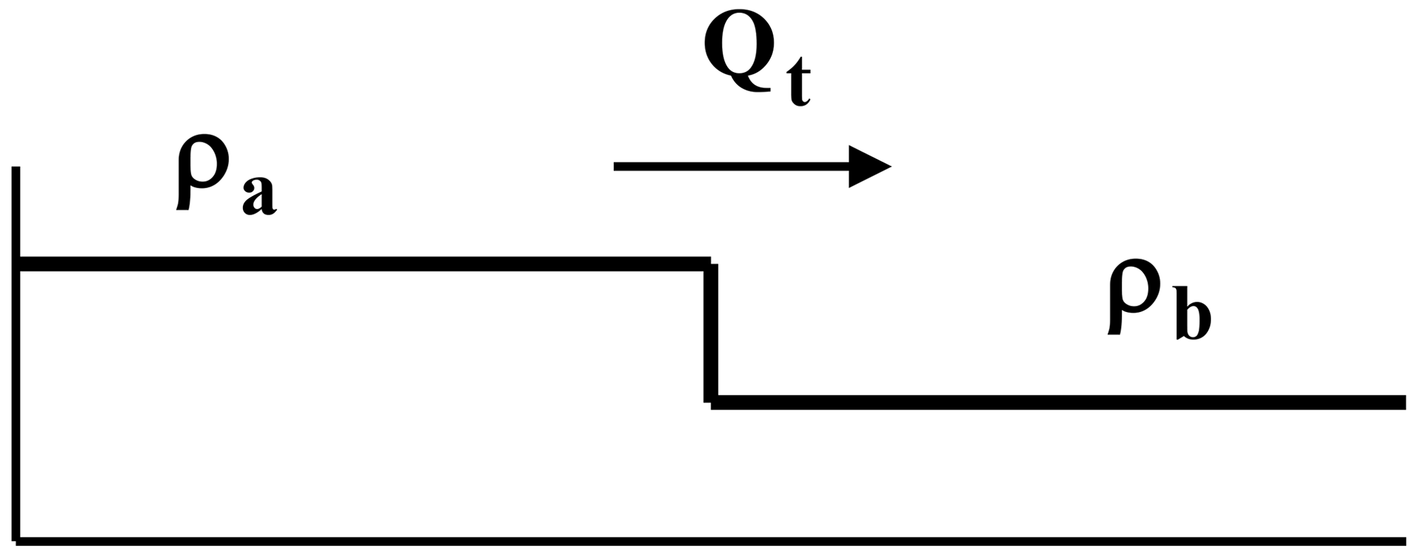
Figure 1 Step initial condition with a density ρ_a at the left of the origin and ρ_b at the right of the origin.

Define the cumulant generating function $\langle e^{\mathit{\lambda }Q}\rangle \simeq e^{\surd t\mathit{\mu }\left(\mathit{\lambda }\right)}$ where λ is a real parameter and 〈,〉 now stands for stochastic average. The functions Φ(q) and μ(λ) are Legendre transform of each other. This problem was studied by Derrida and Gerschenfeld (2009a, b).

The variational equations are

$$\begin{array}{}\text{(38)}& \begin{array}{l}{\displaystyle }{\partial }_t\mathit{\rho }={\partial }_x({\partial }_x\mathit{\rho }-\mathit{\chi }(\mathit{\rho }\left){\partial }_{x}H\right),\\ {\displaystyle }{\partial }_{t}H=-{\partial }_x^{\mathrm{2}}H-{\displaystyle \frac{\mathrm{1}}{\mathrm{2}}}{\mathit{\chi }}^{\prime }\left(\mathit{\rho }\right){\partial }_x^{\mathrm{2}}H,\end{array}\end{array}$$

where χ(ρ) is the mobility. Notice that the equation for H is backward in time, the boundary conditions being $H(t,x)=\mathit{\lambda }\mathit{\theta }\left(x\right)$ and $H(\mathrm{0},x)=\mathit{\lambda }\mathit{\theta }\left(x\right)+f^{\prime }\left(\mathit{\rho }\right(\mathrm{0},x\left)\right)-f^{\prime }\left(\overline{\mathit{\rho }}\right))$, f(ρ) is the equilibrium free energy density.

In Derrida and Gerschenfeld (2009b), the authors calculated the moment generating function with quenched and fluctuating initial conditions, microscopically with the Bethe ansatz and macroscopically with the MFT. The variational equations could be solved only in special cases. Recently Mallick–Moriya–Sasamoto (Mallick et al., 2022) have discovered that the following non-local transformations, which generalize the Cole–Hopf transformation, allow to map the variational equations for the SSEP to the Ablowitz–Kaup–Newell–Segur (AKNS) equations:

$$\begin{array}{}\text{(39)}& {\displaystyle }u(t,x)={\displaystyle \frac{\mathrm{1}}{{\mathit{\chi }}^{\prime }\left(\mathit{\rho }\right)}}{\partial }_x\mathit{\chi }\left(\mathit{\rho }\right)\exp \left[-\underset{-\mathrm{\infty }}{\overset{x}{\int }}\mathrm{d}y{\displaystyle \frac{{\mathit{\chi }}^{\prime }\left(\mathit{\rho }\right)}{\mathrm{2}}}{\partial }_{y}H\right],\text{(40)}& {\displaystyle }v(t,x)=-{\displaystyle \frac{\mathrm{2}}{{\mathit{\chi }}^{\prime }\left(\mathit{\rho }\right)}}{\partial }_x\exp \left[\underset{-\mathrm{\infty }}{\overset{x}{\int }}\mathrm{d}y{\displaystyle \frac{{\mathit{\chi }}^{\prime }\left(\mathit{\rho }\right)}{\mathrm{2}}}{\partial }_{y}H\right].\end{array}$$

The AKNS equations,

$$\begin{array}{}\text{(41)}& {\displaystyle }{\partial }_{t}u(t,x)={\partial }_{xx}u(t,x)-\mathrm{2}{u}^{\mathrm{2}}(t,x)v(x,t),\text{(42)}& {\displaystyle }{\partial }_{t}v(t,x)={\partial }_{xx}v(t,x)-\mathrm{2}{v}^{\mathrm{2}}(t,x)u(x,t),\end{array}$$

were solved for the SSEP, that is $\mathit{\chi }=\mathit{\rho }(\mathrm{1}-\mathit{\rho })$, with the inverse scattering method. These transformations are valid for quadratic χ. The boundary conditions for the step initial condition are

$$\begin{array}{}\text{(43)}& \begin{array}{l}u(\mathrm{0},x)=\mathit{\omega }\mathit{\delta }\left(x\right)\\ v(t,x)=\mathit{\delta }\left(x\right).\end{array}\end{array}$$

From their solution, they obtained the moment generating function

$$\begin{array}{}\text{(44)}& \mathit{\mu }\left(\mathit{\lambda }\right)={\displaystyle \frac{\mathrm{1}}{\surd \mathit{\pi }}}\sum _{\mathrm{1}}^{\mathrm{\infty }}{\displaystyle \frac{(-\mathrm{1}{)}^{n-\mathrm{1}}{\mathit{\omega }}^n}{n^{\mathrm{3}/\mathrm{2}}}},\end{array}$$

where

$$\begin{array}{}\text{(45)}& \mathit{\omega }=(e^{\mathit{\lambda }}-\mathrm{1}){\mathit{\rho }}_a(\mathrm{1}-{\mathit{\rho }}_b)+(e^{-\mathit{\lambda }}-\mathrm{1}){\mathit{\rho }}_b(\mathrm{1}-{\mathit{\rho }}_a).\end{array}$$

For integrability results in the Kipnis–Marchioro–Presutti model of heat transfer, see the recent work by Bettelheim–Smith–Meerson (Bettelheim et al., 2022) and references therein.

5 Final remarks

The MFT shows that once macroscopic evolution equations like hydrodynamics are available and a separation of scales holds, a self-consistent macroscopic description of non-equilibrium phenomena can be obtained through a study of rare fluctuations. The origin of the probabilistic behavior may be due to the influence of a smaller scale on a larger one or to chaotic properties of the underlying dynamical system.

The discovery that a purely macroscopic theory could reproduce in the case of SSEP the large deviation function for non-equilibrium stationary states obtained from a microscopic calculation in Derrida et al. (2002) has been an important support and a source of inspiration for the MFT. The work of Derrida and Gerschenfeld (2009a, b) extended the theory to time-dependent evolutions, and its correctness received an important mathematical support by the recent work of Mallick et al. (2022).

We have illustrated the theory in an idealized case: we have considered (i) purely diffusive systems and (ii) simplified stochastic models. However as the Ising model allowed us to understand a lot about phase transitions and the critical point, we believe that the SSEP and other solvable models are providing a guide to what may happen out of equilibrium. Furthermore the MFT applies to all variants of SSEP or of other diffusive models that macroscopically have the same transport coefficients D,χ.

The general approach of MFT has been extended to systems with more than one conservation law (Bernardin, 2008) and to some reaction diffusion processes like the Glauber–Kawasaki dynamics (Jona-Lasinio et al., 1993; Bodineau and Lagouge, 2010). It is reasonable to expect that it will be applicable to more general cases, which may lead to a different structure of the large deviation rates.

The experience so far indicates that the phenomenon of long-range space correlations is not limited to purely diffusive systems and is rather general in non-equilibrium.

In climate science, the models are comparatively more complicated. However the application of large deviation theory to rather complex models as in Galfi et al. (2019), Galfi and Lucarini (2021), Galfi et al. (2021) and Lucarini et al. (2022) is encouraging.

Appendix A: Fluctuating hydrodynamics

Formally, the equations of the MFT can be derived also from assuming an extension to non-equilibrium of the so-called fluctuating hydrodynamics (FHs). The idea of fluctuating hydrodynamics goes back to Landau (Landau and Lifshitz, 1980) who considered only linear hydrodynamic equations near equilibrium, while the most interesting phenomena are generated by non-linearities far from equilibrium. It consists in adding to the macroscopic equations a noise term. In the case of hydrodynamic equations in divergence form, we add to the current a fluctuating term,

$$\begin{array}{}\text{(A1)}& j=J\left(\mathit{\rho }\right)+\mathit{\xi },\end{array}$$

where, conditionally on ρ, ξ is a Gaussian random term with variance as follows:

$$\begin{array}{}\text{(A2)}& \langle {\mathit{\xi }}_i(t,x),{\mathit{\xi }}_j(t^{\prime },x^{\prime })\rangle ={\mathit{ϵ}}^d{\mathit{\chi }}_{ij}\left(\mathit{\rho }\right)\mathit{\delta }(t-t^{\prime })\mathit{\delta }(x-x^{\prime }).\end{array}$$

The hydrodynamic equation takes the following form:

$$\begin{array}{}\text{(A3)}& {\partial }_t\mathit{\rho }+\mathrm{\nabla }\left(J\right(\mathit{\rho })+\mathit{\xi })=\mathrm{0}.\end{array}$$

However we have to emphasize that such equations, in the case of non-linear hydrodynamics, are very singular and need renormalization, and so far there is no mathematical theory applicable even in one dimension.

From the previous equations, we obtain

$$\begin{array}{rl}\mathbf{P}(\mathit{\rho },j)& \asymp \exp \mathit{\{}-{\displaystyle \frac{\mathrm{1}}{{\mathit{ϵ}}^d}}{\displaystyle \frac{\mathrm{1}}{\mathrm{4}}}\int \mathrm{d}t\int \mathrm{d}x(j-J\left(\mathit{\rho }\right))\cdot \mathit{\chi }(\mathit{\rho }{)}^{-\mathrm{1}}(j-J(\mathit{\rho }\left)\right)\mathit{\}}\\ & =\exp \mathit{\{}-{\displaystyle \frac{\mathrm{1}}{{\mathit{ϵ}}^d}}{\mathcal{I}}_{[t_{\mathrm{0}},t_{\mathrm{1}}]}(\mathit{\rho },j\left)\mathit{\right\}},\end{array}$$

the same as formula (18).

It would be interesting to provide a rigorous foundation to fluctuating hydrodynamics; however this requires as a first step to give a clear mathematical meaning to the stochastic partial differential equations on which it is founded.