the Creative Commons Attribution 4.0 License.
the Creative Commons Attribution 4.0 License.
 | 22 Jun 2023
Reducing manipulations in a control simulation experiment based on instability vectors with the Lorenz-63 model
Mao Ouyang
Keita Tokuda
Shunji Kotsuki
Controlling weather is an outstanding and pioneering challenge for researchers around the world, due to the chaotic features of the complex atmosphere. A control simulation experiment (CSE) on the Lorenz-63 model, which consists of positive and negative regimes represented by the states of variable x, demonstrated that the variables can be controlled to stay in the target regime by adding perturbations with a constant magnitude to an independent model run (Miyoshi and Sun, 2022). The current study tries to reduce the input manipulation of the CSE, including the total control times and magnitudes of perturbations, by investigating how controls affect the instability of systems. For that purpose, we first explored the instability properties of Lorenz-63 models without and under control. Experiments show that the maximum growth rate of the singular vector (SV) reduces when the variable x was controlled in the target regime. Subsequently, this research proposes to update the magnitude of perturbations adaptively based on the maximum growth rate of SV; consequently, the times to control will also change. The proposed method successfully reduces around 40 % of total control times and around 20 % of total magnitudes of perturbations compared to the case with a constant magnitude. Results of this research suggest that investigating the impacts of control on instability would be beneficial for designing methods to control the complex atmosphere with feasible manipulations.
- Article
(5167 KB) - Full-text XML
- BibTeX
- EndNote


The ability to control the future based on past and present data is of interest in geophysics, e.g. reducing extreme and rare events, controlling climate changes, and changing cyclone tracks (Lucarini et al., 2016). Miyoshi and Sun (2022) proposed a control simulation experiment (CSE) to change the future by applying perturbations to the independent model run. Their experiments successfully controlled the state variable x in the positive regime of the Lorenz-63 model (Lorenz, 1963; Miyoshi and Sun, 2022). Sun et al. (2022) conducted CSEs on the Lorenz-96 models (Lorenz, 1996), results of which demonstrated that the CSE can be employed to control the occurrences of extreme events. The goal of CSE is to control the real-world weather (Miyoshi and Sun, 2022), whereas only preliminary investigations were reported in small-scale dynamic models (Miyoshi and Sun, 2022; Sun et al., 2022). The fundamental principles behind the mechanism of controlling the weather remain obscure. Specifically, reducing the control times and the magnitudes of the perturbations are two key challenges for a successful implementation of CSEs to complex dynamic systems, which were not thoroughly examined yet. Here, we investigate two types of vectors, namely, bred vector (BV) and singular vector (SV), which are frequently used to explore the instability properties of chaotic models, to try to find feasible manipulations for CSE in the Lorenz-63 model.
The breeding method was proposed to estimate dynamic forecast errors in atmospheric models (Toth and Kalnay, 1993, 1997). BV represents the nonlinear initial error growth within short- and medium-range periods by minimal computation effort. Zhang et al. (2015) demonstrated that the Lorenz-63 model has two different bred vectors, which would converge to one when a small random noise was added to the perturbations at each breeding cycle (Corazza et al., 2003). Singular vector (SV) was defined as the fastest growing perturbations through singular value decompositions of an operator, e.g. tangent linear model (TLM) (Diaconescu and Laprise, 2012). The initial perturbations in an ensemble prediction system at the European Centre for Medium-Range Weather Forecasts (ECMWF) were constructed by SVs, due to which produced dispersive ensembles with the most unstable directions (Palmer, 2019). Kim and Jung (2009) identified the regions sensitive to small perturbations in a tropical cyclone by SV. The growth rates of BV and SV were reported to be able to predict the regime changes in the Lorenz-63 model (Evans et al., 2004; Norwood et al., 2013). The calculation of BV and SV could be independent of the infinite time trajectory, which meets the essential criteria of CSE (Miyoshi and Sun, 2022); thus, we examined their properties.
The present study investigates the impacts of control in the Lorenz-63 model on BV and SV and discusses the approach of introducing these vectors to determine feasible manipulations in CSE. We first review the approach of CSE briefly (Miyoshi and Sun, 2022), and we describe the methods for calculating BV and SV. Then, two trajectories of the Lorenz-63 model, one without control and the other one with control activated at a certain time, are calculated. We compare the BVs and the SVs of the two trajectories at the initial stage of activating control and during a long time period. Based on the features of vectors, we will discuss possible approaches to adaptively determine the manipulations in CSE.
2.1 Lorenz-63 model
The model used in this study is the Lorenz-63 model, given by
where the standard parameters α = 10, ρ = 28, and β = are selected for chaotic behaviour with two regimes i.e. the famous butterfly pattern (Lorenz, 1963). The initial condition is chosen as (x, y, z) = (8.20747939, 10.0860429, 23.86324441) following Miyoshi and Sun (2022). Nature run (NR) is obtained by integrating the Lorenz-63 model for 208 000 time steps using the fourth-order Runge–Kutta scheme with a time step increment (dt) of 0.01. Hereafter in this paper, we use the number of these discretised time steps as the time parameters. We save the NR for 208 000 time steps, because it could provide sufficiently long reference data for evaluating the data assimilation results and provide many starting points for investigating the characteristics of CSEs under various conditions. This trajectory is named as xn, where subscript n represents NR without control.
2.2 Control simulation experiment
The CSE is an output feedback control method that determines manipulations based on outputs (or signals) from the system. In the framework by Miyoshi and Sun (2022), the output is observation data generated from NR. To estimate accurate analysis, the CSE needs to employ sequential data assimilation cycles. This study implements the ensemble Kalman filter (EnKF) (Bishop et al., 2001; Houtekamer and Zhang, 2016) following Miyoshi and Sun (2022). Three initial forecast ensembles are obtained by adding random Gaussian noise r∼𝒩 (5.0, 1.0E) to NR (Kalnay et al., 2007), where E is the identity matrix, 5.0 denotes the vector (5, 5, 5)T, and 𝒩 (5.0, Σ) denotes the multivariate normal distribution applied throughout the paper and defined as below:
Observations are generated every Ta = 8 time steps by adding Gaussian noise 𝒩 (0.0, 2.0E) to NR, and they are assimilated in the data assimilation cycle. Multiplicative inflation of the EnKF is manually tuned to be 1.04, which is consistent with previous studies (Kalnay et al., 2007). The first 8000 time steps, corresponding to 1000 data assimilation cycles, are discarded to ensure that the root mean square error (RMSE) of the mean of ensemble forecast and NR is around 0.30 (Yang et al., 2012). The purpose of the ensemble data assimilation cycle is to obtain ensemble forecasts for determining manipulations in CSE.
The goal of CSE is to control state variable x to stay in the positive regime by adding perturbations to NR. The process designed by Miyoshi and Sun (2022) is reviewed as follows:
-
Perform a data assimilation based on observations at time t.
-
Employ an ensemble forecast for T time steps from t to t+T.
-
If at least one ensemble member changes the regime, control (step 4) will be activated; otherwise, data assimilation at time t+Ta will be performed for the next cycle (step 1).
-
Perturbations are defined as the differences between the ensemble forecasts with and without regime changes. If all three ensemble members show regime change, former initial ensembles will be forecasted for extended time steps to identify at least one ensemble member showing no regime change from t to t+T. The perturbations normalised by constant Euclidean norm D are added to NR at every time step from t+1 to . The new NR, i.e. NR with adding perturbations, is used to generate observations for the subsequent data assimilation cycle (step 1).
The forecast time period T and Euclidean norm of perturbations D are tunable parameters in CSE. The ratio of successful control was high when T=300 time steps and D=0.05 (Miyoshi and Sun, 2022); thus, we adopt these parameters in this study. The trajectory under control by CSE is named as xc, where the subscript c represents NR under control.
2.3 Bred vector
Of the two types of vectors, the BV is the easier and faster to compute. We need to define the trajectory of interest xi, which is xn or xc in this study. Figure 1a and b show the methods for calculating BV without and under control. At the beginning of breeding cycle at time t, a perturbation p, scaled to size δ, and a Gaussian noise r∼𝒩 (0, 0.1E) (Corazza et al., 2003), are added to the trajectory xi(t).
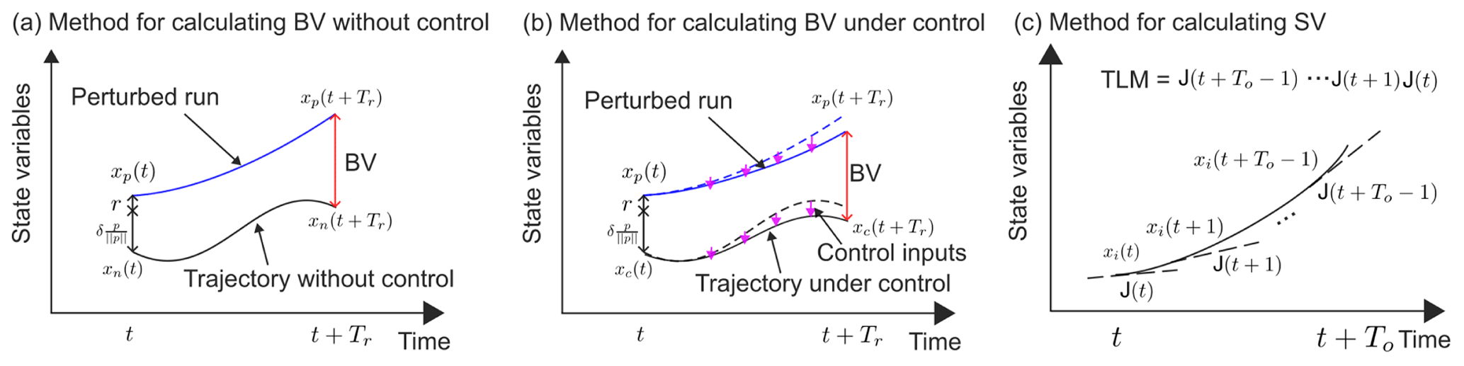
Figure 1Methods for calculating (a) BV without control, (b) BV under control, and (c) SV in general case. Please refer to the text for the meaning of each parameter.
The initial condition for the perturbed trajectory xp(t), at time t, will be
where is the Euclidean norm of p. The Lorenz-63 model is then used to integrate the perturbed trajectory forward starting from xp(t) for both trajectories without control xn and under control xc. For the trajectory under control xc, the influence of control inputs in CSE accumulates over multiple time steps. To examine the influence of the perturbation () on the systems without and under control, we add the same control inputs (the purple arrows in Fig. 1b) to the perturbed run as the independent run xc for calculating the BV. At the end of the rescaling interval Tr, BV can be obtained by subtracting xi(t+Tr) from the perturbed trajectory,
The process is repeated from Eq. (5) with as the perturbation for the next breeding cycle. The growth rate of BV is calculated by , where is the Euclidean norm of BV. The main parameters of BV are the perturbation size δ and rescaling interval Tr, which represent the effects of linear and nonlinear disturbances on error growth. We set δ equal to 1.0 and Tr equal to 8 time steps following Evans et al. (2004). The growth rate of BV is calculated once every Tr = 8 steps when the norm of BV is normalised. To obtain an instantaneous BV growth rate at every time step, we used parallel BVs, each normalised successively at different time steps along the trajectory.
2.4 Singular vector
The vectors which maximise the growth rate of perturbations for a chosen norm and optimisation time interval (To) can be represented by SV. The process of finding SV for a given state (xn or xc) starts with the Jacobian matrix (Diaconescu and Laprise, 2012), which for the Lorenz-63 model at a given state (x(t), y(t), z(t)) is given by
For simplicity, we set To equal to 1 time step, i.e. 0.01 time units. The SV can be calculated through the singular value decomposition of Jacobian matrix (Eq. 7) as
where U and V are orthonormal matrices (Press et al., 1992), VT denotes the conjugate transpose of V, and is a diagonal matrix with descending non-negative singular values. We calculate the first column of V, which is the initial leading SV, corresponding to the fastest growing vector from time t to t+1. Euclidean norm is employed to compute the growth rate of SV, which is given by ln s11.
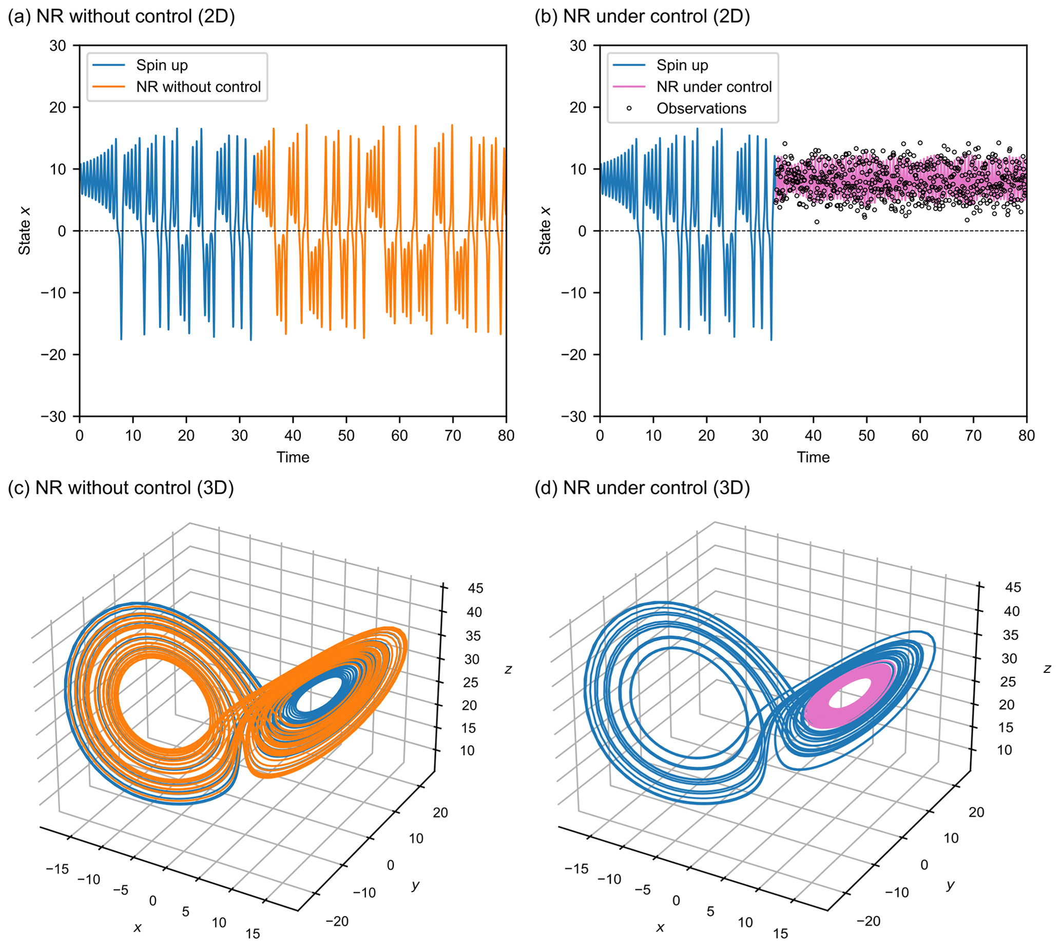
Figure 2State variables of the Lorenz-63 model. (a) State variable x in 2D plane without control. (b) After control, state variable x stays in the positive regime. The empty circles represent the observations generated by CSE. (c) Lorenz's butterfly attractor from NR, i.e. no control (xn). (d) Trajectory under control (xc). Blue line represents the spin-up states. Orange and magenta lines represent the NR without and under control, respectively. Initial control is activated at the time of 32.89.
We show the general case of calculating SV for dynamic models in Fig. 1c. The singular value decomposition is conducted in the TLM by the production of Jacobian matrices. In this study, the Jacobian matrices for both trajectories without and under control (xn and xc) are calculated by Eq. (7), assuming that the manipulations applied in the CSE can be regarded as an external force that would not affect the linear propagation of perturbations.
3.1 Control simulation experiment
We first conduct the experiments to confirm that CSE can control the state variable x to the target regime. Experimental results without control, i.e. trajectory with orange lines (xn), and under control, i.e. trajectory with magenta lines (xc), are shown in Fig. 2. Spin-up states refers to the initial period taken before the control is activated where the variables might suffer from transit effects (Lorenz, 1996), which are shown as blue lines in Fig. 2. Observation of Fig. 2b and d demonstrates that CSE can successfully generate observations and control the state variable x in the positive regime.
We calculate BV and SV of the two trajectories, xn and xc, based on the methods described in Sect. 2. To investigate the influence of control on the vectors, we focus on the instantaneous changes of vectors when control is activated and the changes of vectors during a long time period, which will be shown subsequently.
3.2 Influence of starting point on CSE
Lorenz (1963) noted that when the state variable x shows large values, the trajectory tends to change regimes. This suggests that if the starting point of the control is near the extreme value of x, it may be more difficult to control the state variables in the target regime. Here, we conduct 400 CSEs with different starting points randomly sampled in between the time unit of 50 and 150. When the state value x of the starting points is positive, the CSEs are performed for 8000 time steps, i.e. 1000 data assimilation cycles. Figure 3 shows the relationship between the number of successful and failed CSEs and the state variable x when the initial control is activated. If the control is activated at state variable x in the range of 15–20, the failed probability is quite high. For the successful controls, the initial controls occurred in the range from 0 to 15.
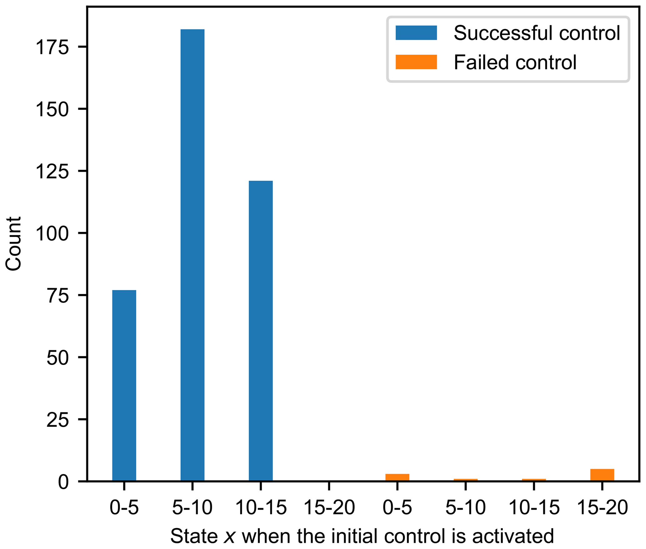
Figure 3The numbers of successful and failed CSEs with the state variable x when the initial control is activated.
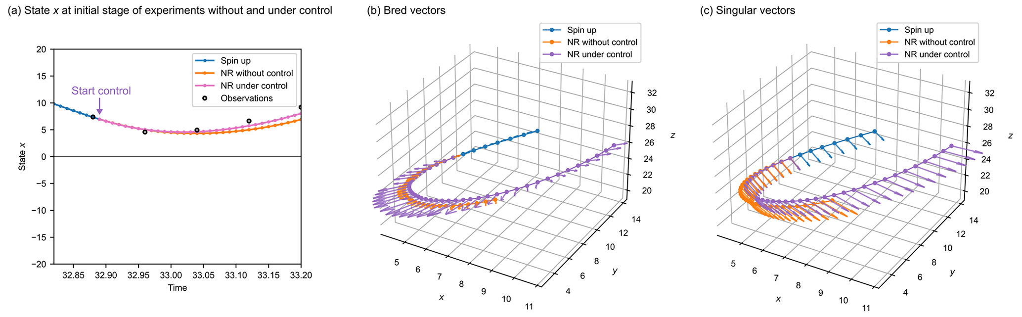
Figure 4Experimental results of changes in two vectors at the initial stage of CSE. (a) State x at the initial stage of experiments without and under control. The empty circles represent the observations generated by CSE. (b) The BVs. The lengths of the vectors represent the growth rate of BV with a magnification of 20. (c) The SVs. The lengths of the vectors represent the growth rate of SV with a magnification of 50. Blue line represents the spin-up states. Orange and magenta lines represent the NR without and under control, respectively. Control is activated at time 32.89.
3.3 Influence of control at the initial stage
Figure 4 shows the vector changes without and under control at the initial stage of experiments. After discarding the first 8000 time steps, we start the CSE; the initial control is activated at the time of 32.89. Figure 4a shows the time to start control and the different trajectories without and under control by orange lines xn, and magenta lines xc, respectively. The empty circles are the observations generated by the CSE, which are all located in the target regime. Figure 4b and c show changes in BV and SV for experiments without and with control inputs. The lengths of the vectors represent the growth rates of BVs and SVs, which are enlarged by a factor of 20 and 50 for better visualisation, respectively. When the control inputs are added to the model, both the direction and magnitude of BV are changed due to the fact that the external forces would change the nonlinear error propagations for Tr time steps, i.e. 8 time steps. The directions and magnitudes of SV are similar for those without and under control (Fig. 4c). This is because both NRs without and under control during the selected period do not show the trend to change regimes. Therefore, even though the control inputs are added to the NR under control, the direction and magnitude are similar to those of NR without control.
3.4 Influence of control during a long time period
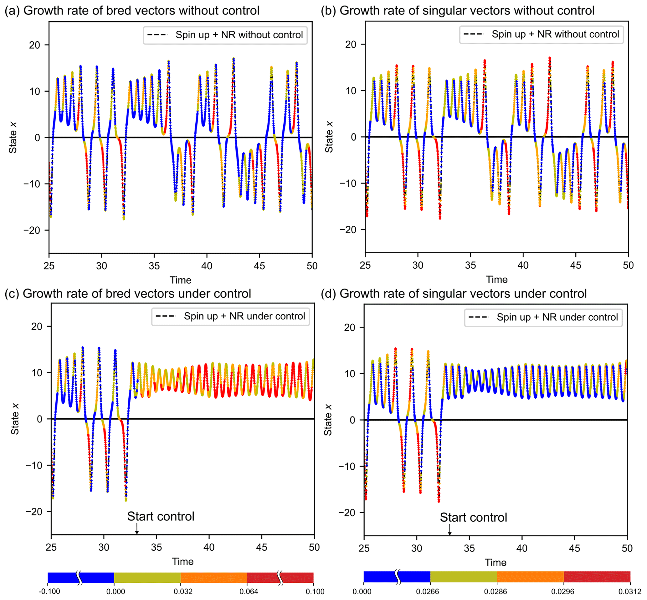
Figure 5Experimental results for long time period. Growth rates of BV (a) without control and (c) under control. Growth rates of SV (b) without control and (d) under control. Control is activated at time 32.41. The dashed black lines are the trajectories of interest, xn and xc. Coloured stars in (a) and (c) represent the growth rate of BV, with absolute value shown in the colour bar below (d). Coloured stars in (b) and (d) represent the growth rate of SV, with absolute value shown in the colour bar below (e).
It was reported that the regime changes of the Lorenz-63 model can be predicted by the growth rates of BV (Evans et al., 2004) and SV (Norwood et al., 2013). In the case of BV, the regime change was predicted by the growth rate, i.e. when the growth rate in current cycle exceeds 0.064, the next cycle will change to the other regime (Evans et al., 2004). Norwood et al. (2013) reported that the growth rate of SV also implied regime changes, i.e. when the growth rate of SV exceeds 0.0296 in the current cycle, state variable x would change to the other regime in the next cycle.
Table 1Regime change forecast verification of BV and SV. The numbers and those in the brackets represent the percentage of mean and standard deviation to the averaged total number of 100 different time series.
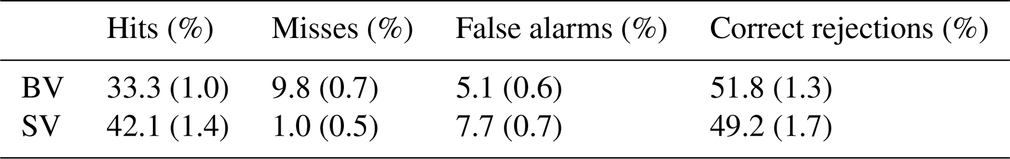
Examined vectors of the trajectory without control are shown in Fig. 5a and b for 2500 time steps. Table 1 shows the forecast verifications (Jolliffe and Stephenson, 2011) based on the rules of regime changes prediction described above, where “hit” means the rule successfully forecasts the observation, “miss” means that regime change is observed but not forecasted by the rule, and “false alarm” means that the rule forecasts a regime change but no regime change occurs; “correct rejection” means that the regime change is neither observed nor forecasted by the rule. The threshold values used here are described in the above paragraph. We verify the forecast for 100 different time series with each verification period equal to 1000 time units, i.e. 100 000 time steps. The percentages of mean values and the standard deviations are shown in Table 1. Results indicate that the growth rate of SV shows better performance than BV regarding the regime change prediction.
The features of BV and SV of trajectory under control are shown in Fig. 5c and d. Characteristics of BV and SV are altered by the control. Figure 5c suggests that the growth rate of BV of the controlled system shows large values despite the absence of regime changes, which gives us two hints. One is that when external forces are added to the Lorenz-63 model, BV may not be able to effectively predict the regime changes. Another one is that the nonlinear error growth of the controlled system is larger than that of the original system, indicating that the CSE might increase the nonlinear features to the chaotic models. Interestingly, the growth rate of SV is reduced after control, e.g. maximum growth rate shows 5 % decrease, i.e. from 0.0312 to 0.0296 (Fig. 5d).
To illustrate the robustness of the reduction of the maximum growth rate of SV, we examined the SV of the successful CSEs with different starting points. The relationship between the state variable x when the initial control is activated and the maximum growth rate of SV is shown in Fig. 6. The maximum growth rates of SV are affected by the starting point. Compared with the cases without control, the maximum growth rate of SV under control presents a great reduction for all CSEs with different starting points. The maximum growth rates of SV under control show a mean value of 0.0296 and a standard deviation of 0.00015. We use the mean value of 0.0296 for our subsequent studies.
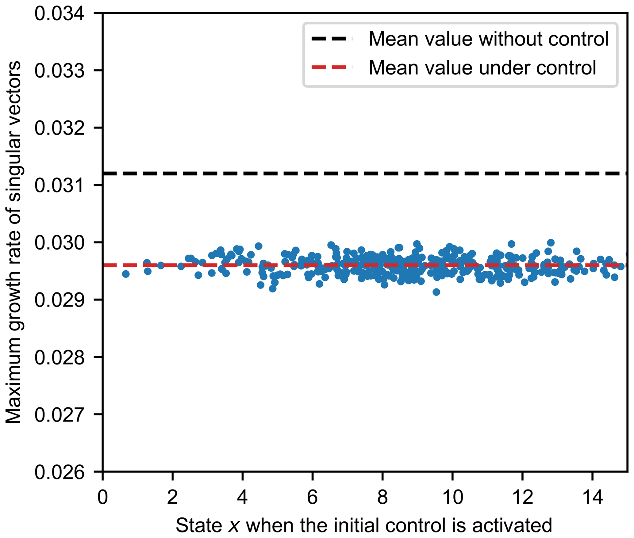
Figure 6Maximum growth rate of SV for the trajectories under control at different starting points.
Our results demonstrated that controlling the state variables changed the characteristics of BV and SV. Here, we will discuss a new approach which could determine feasible manipulations, including total control times and magnitudes of perturbations in CSE, through the insights from the investigations on instability vectors.
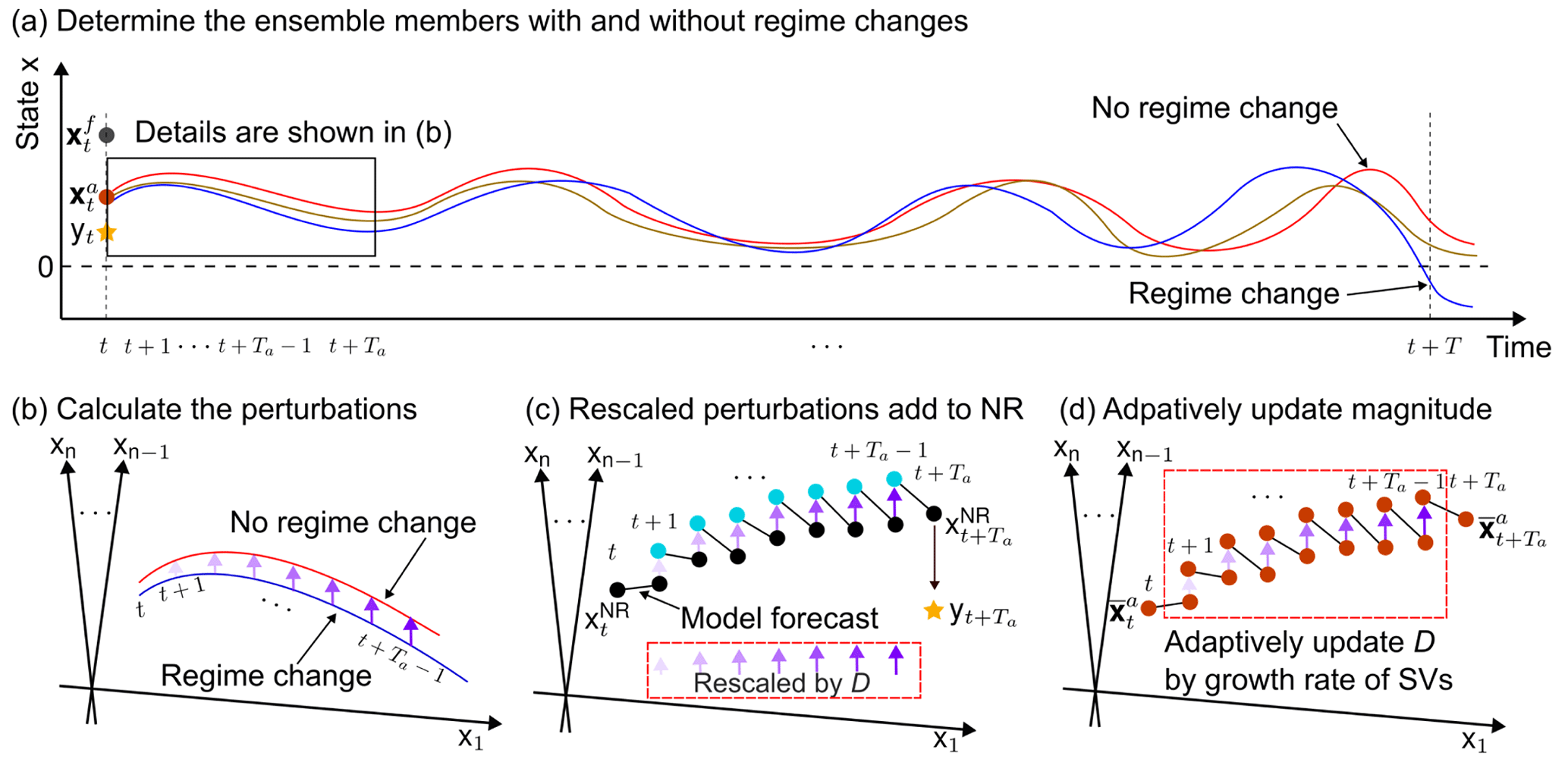
Figure 7Schematic illustrations of the experimental procedures. (a) Determine the ensemble members with and without regime changes. (b) Calculate the perturbations based on the differences of the ensemble forecasts obtained from (a). (c) Rescale the perturbations to magnitude, D, and add them to NR. (d) Adaptively update the magnitude D according to the growth rate of SV of analysis mean. Please note that the axes x1, xn−1, and xn in (b), (c), and (d) represent that the perturbations are multidimensional vectors in this study.
4.1 Introduce growth rate of SV to update magnitude adaptively
Miyoshi and Sun (2022) controlled the state variables by adding a constant magnitude of perturbations to NR in their CSE. The schematic diagram of the process related to manipulation in CSE is shown in Fig. 7a–c. After performing the data assimilation at time t, analysis ensembles are iterated for T time steps to find the ensemble members with and without regime changes (Fig. 7a), the differences of which during t+1 and over 0.08 time units are regarded as perturbations (Fig. 7b). State variables are changed by adding the rescaled perturbations with constant magnitude D to NR from t+1 to (Fig. 7c). Miyoshi and Sun (2022) suggested that the magnitude of perturbation was a sensitive parameter and needed further investigations.
Investigation of SV showed that when the state x was controlled in positive regime, the maximum growth rate of SV was less than 0.0296 (Sect. 3.4). We then proposed to apply this rule in CSEs to update the magnitude of perturbations added to NR adaptively, as shown in Fig. 7d. The perturbations (Fig. 7b) are rescaled with initial Euclidean norm D = 0.010, and they are added to the integration of analysis mean , which is the mean value of the analysis ensembles after the data assimilation (step 1 of CSE) from t+1 to . We calculate the growth rates of SVs for these Ta−1 time steps. The magnitude D is determined until the maximum growth rate of SVs was less than 0.0296; otherwise, increase D by 0.001. The process will finish after either finding D which meets the requirement or D reaching the boundary which is assumed as the maximum possible intervention.
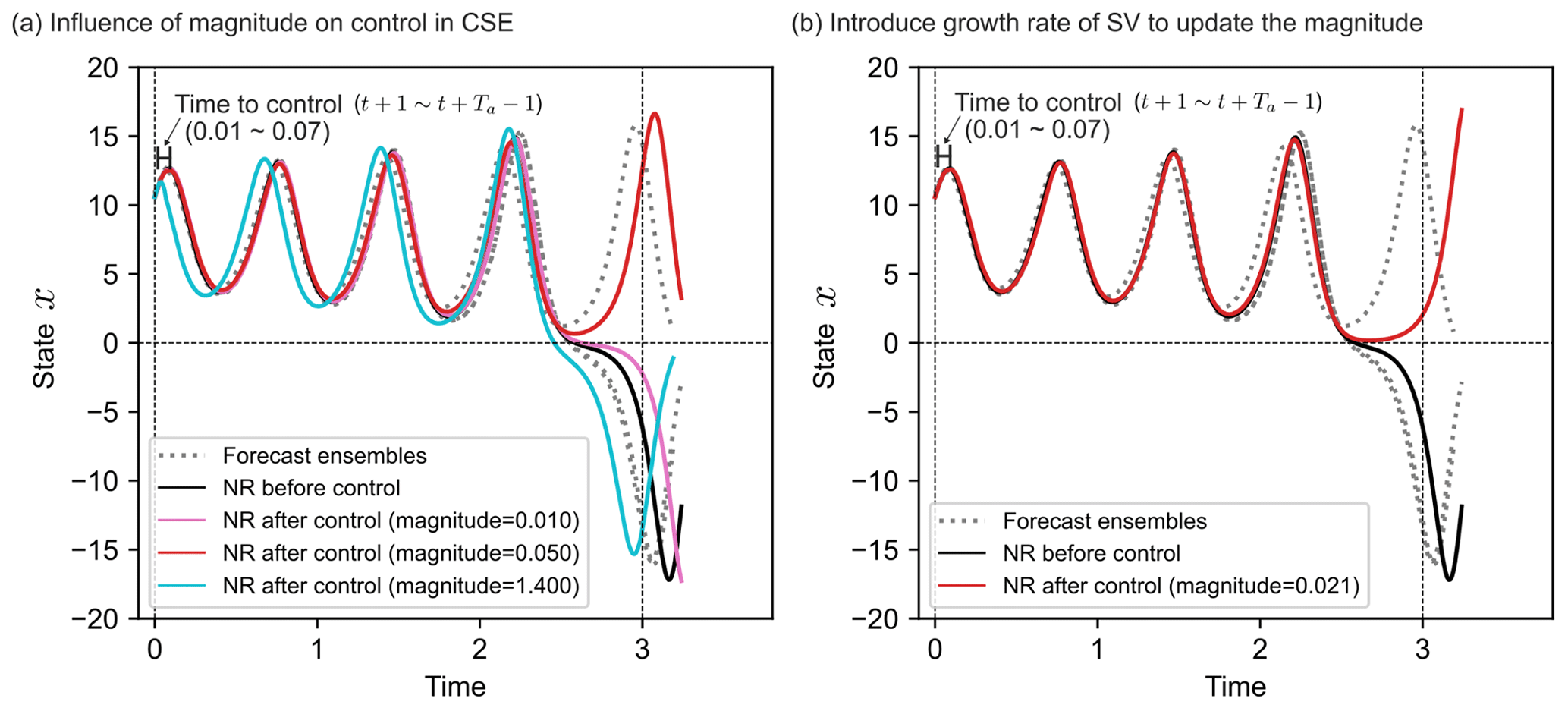
Figure 8Introducing growth rate of SV to control the state variables. (a) Influence of magnitudes on the control in CSE. (b) Introduce growth rate of SV to calculate the necessary magnitudes. The grey dotted lines are the forecast ensembles. Black lines represent the NR before control. Perturbations are added to NR from time 0.01 to 0.07 over 7 time steps. The purple and cyan lines represent the NR after control with constant magnitude of perturbations 0.010 and 1.400, respectively. The red line in (a) represents the NR after control with subjectively determined constant magnitude of perturbation 0.050. The red line in (b) represents the NR after control with magnitude of perturbations determined by growth rate of SV, 0.021.
We conduct experiments with only one data assimilation cycle to investigate the applicability of growth rate of SV in CSE. When D is subjectively determined, Fig. 8a shows that the cases with too small (0.010) and too large (1.400) magnitudes cannot successfully control the state x in positive regime, whereas that with magnitude 0.050 can achieve the goal. If D is determined by the growth rate of SV, Fig. 8b notes that the necessary magnitude to control state x in positive regime is only 0.021. This test elaborates that the growth rate of SVs can be applied in CSE to successfully control state variables.
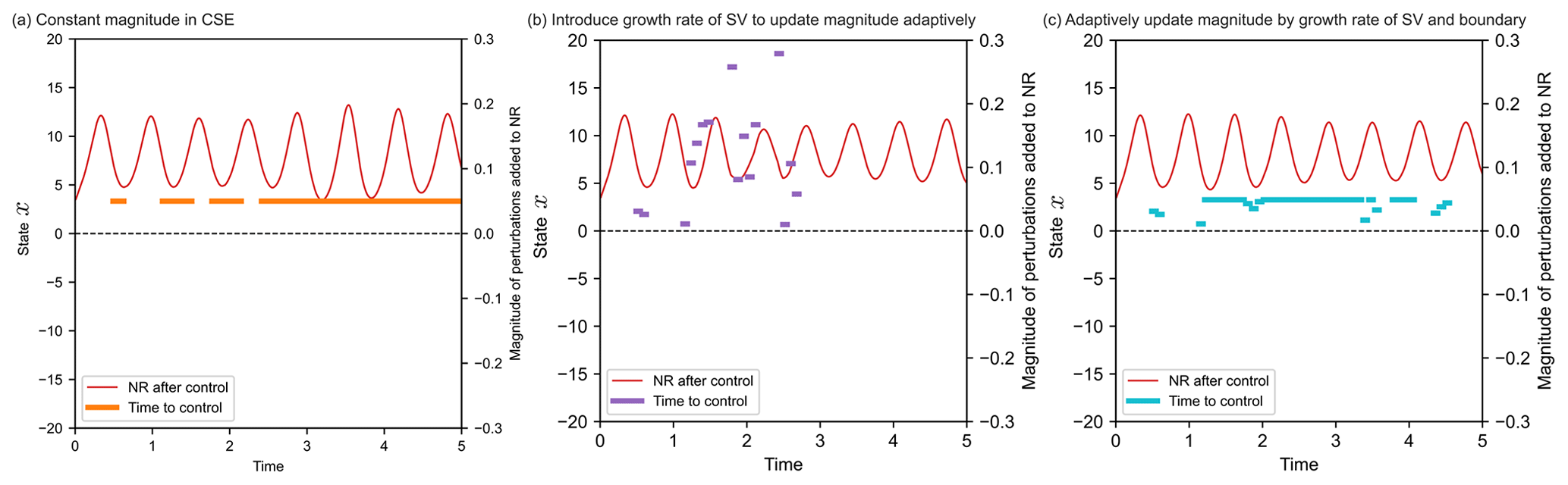
Figure 9Comparison between constant and adaptive magnitudes in CSE for 500 time steps. (a) Constant magnitude in CSE. (b) Introduce the growth rate of SV to update the magnitudes adaptively. (c) Adaptively update the magnitude by growth rate of SV and boundary. The red lines represent the NRs after control. The thick orange, magenta, and blue lines represent the times to activate control by constant magnitude (a), adaptive magnitude without boundary (b), and adaptive magnitude with boundary (c), respectively.
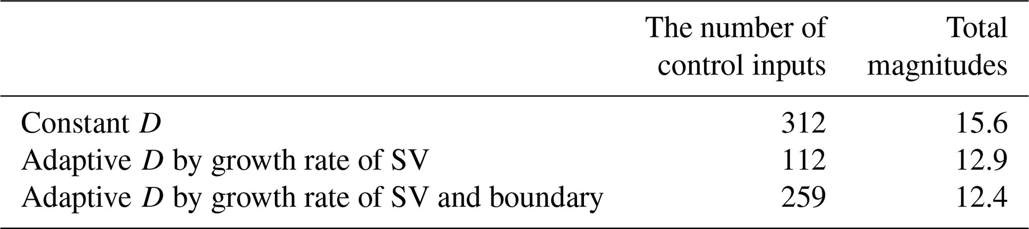
Table 2Comparison between constant and adaptive magnitudes for 500 time steps.
4.2 Comparison between constant and adaptive magnitudes
To investigate the influence of adaptive magnitude on the total control times and magnitudes of perturbations, we conduct CSEs with constant magnitude, 0.05, as recommended by Miyoshi and Sun (2022); adaptive magnitude without boundary; and adaptive magnitude with boundary to be 0.05, for 500 time steps. The results are shown in Fig. 9 and Table 2. The total control times reduce from 62.4 % (312 out of 500) to 22.4 % (112 out of 500) if the growth rate of SV was implemented to update the magnitude adaptively. The case with adaptive magnitude and boundary shows around 20 % decrease of total magnitudes of perturbations compared to that with constant magnitude.
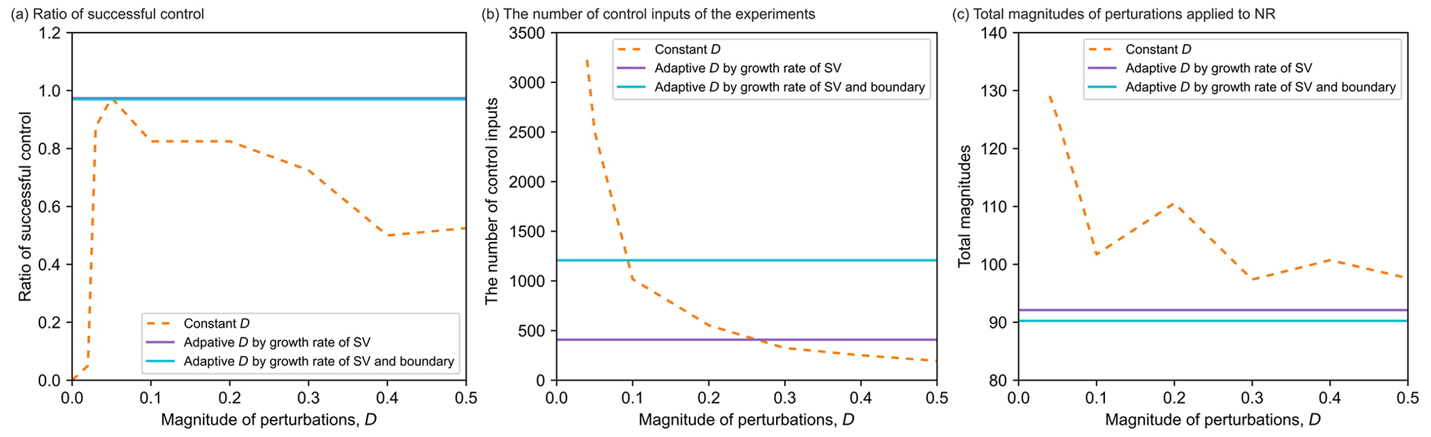
Figure 10Comparison between constant and adaptive magnitudes in terms of (a) Ratio of successful control; (b) Times to control; (c) Total magnitudes. The orange dashed, magenta, and blue lines represent the results of constant D, adaptive D by growth rate of SV, and adaptive D by growth rate of SV and boundary, respectively. Please note that the magenta and blues lines are the results with adaptive D, which are not dependent on the prescribed D and are shown as horizontal lines in this figure.
We conduct 40 experiments for 8000 time steps, corresponding to 1000 data assimilation cycles, to examine the performance of adaptive magnitude and the sensitivity of D for constant magnitude, as shown in Fig. 10. The rate of successful control is calculated as the ratio of cases when NR is controlled in the target regime. Figure 10a shows that the rate of successful control for adaptive magnitude was around 97.5 %, suggesting only 1 case fails out of 40. Total control times by adaptive magnitude without boundary are reduced from those by constant magnitude, when the applied constant magnitudes are smaller than 0.200 (Fig. 10b). Total control times of cases with adaptive D by growth rate of SV and boundary are larger than those with only adaptive D by growth rate of SV (blue and magenta lines in Fig. 10b). The experiment with adaptive magnitude by growth rate of SV and boundary achieves the minimal total magnitudes of perturbations, around 90.6, among all experiments in this study (Fig. 10c).
We investigated the impacts of control on two vectors related to instability, i.e. bred vector and singular vector in the Lorenz-63 model. Results demonstrate that the features of these vectors will change if the state variables are controlled to the target regime. The maximum growth rate of the singular vectors shows around 5 % decrease after control and is introduced to calculate the magnitude of perturbations in control simulation experiments. Accordingly, the manipulation, including total control times and magnitudes of perturbations, is designed to be updated adaptively based on the maximum growth rate of singular vectors. Total control times and magnitudes of perturbations show around 40 % and 20 % reduction, respectively, when updating the magnitude adaptively, which indicates that the manipulations are reduced through the method proposed in this research.
The information of bred vector and singular vector may be possible to be applied to reduce the time of control and magnitude of perturbations for the general cases, including but not limited to the Lorenz-63 model and regime changes. The control simulation experiment was designed to control the weather which shows separatrices, e.g. the separations between a normal precipitation and a heavy rainstorm or the separations of typhoon moving east and moving west, etc. The instability vectors probably show drastic changes near these separatrices, which might give us the chance to find effective ways for reducing the manipulations in the control simulation experiment.
Control of the state variables of the Lorenz-63 model is a simplified scenery of meteorological study. For complex dynamic systems, e.g. a full-scale numerical weather prediction model, caution is necessary when applying the proposed method to control the weather. For example, it is difficult to explicitly obtain the tangent linear model in medium- and large-scale atmospheric models, and a larger number of ensemble size would cause a higher probability for the ensemble forecasts to be in the undesired regimes; thus, more studies are necessary on the adaptive manipulation update. The present study throws light on the introduction of instability vectors to find optimal manipulations for the control simulation experiment. Climate-change-induced extreme weather, e.g. typhoon, storm surge, intensive rainfall, was reported to cause catastrophes in recent years (Kotsuki et al., 2019; Ouyang et al., 2021, 2022). Covariant Lyapunov vectors could provide insights into the spatio-temporal instability of chaotic systems (Egolf et al., 2000). Future research will be focused on exploring the chaotic features by covariant Lyapunov vectors (Ginelli et al., 2007; Tokuda et al., 2019, 2021) and implementing these vectors in atmospheric models to control extreme weather for mitigating natural hazards.
The code that supports the findings of this study is available from the corresponding authors upon reasonable request.
The authors declare that all data supporting the findings of this study are available within the figures and tables of the paper.
MO and SK conceived of the study. SK is the principal investigator. MO conducted the numerical experiments and wrote the manuscript. KT analysed the results. All authors contributed to framing and revising the paper.
The contact author has declared that none of the authors has any competing interests.
Publisher's note: Copernicus Publications remains neutral with regard to jurisdictional claims in published maps and institutional affiliations.
The authors thank project members of the Moonshot JPMJMS2284 for fruitful discussion.
This research has been supported by the Japan Science and Technology Agency (grant no. MJPR1924); the Japan Society for the Promotion of Science (grant nos. JP21H04571, JP22K18821, JP20K19882, and JP23K11259); the Moonshot Research and Development Program (grant no. JPMJMS2284); the Ministry of Education, Culture, Sports, Science and Technology (grant no. JPMXP1020200305); and the IAAR Research Support Program of Chiba University.
This paper was edited by Pierre Tandeo and reviewed by two anonymous referees.
Bishop, C. H., Etherton, B. J., and Majumdar, S. J.: Adaptive sampling with the ensemble transform Kalman filter. Part I: Theoretical aspects, Mon. Weather Rev., 129, 420–436, https://doi.org/10.1175/1520-0493(2001)129<0420:ASWTET>2.0.CO;2, 2001. a
Corazza, M., Kalnay, E., Patil, D. J., Yang, S.-C., Morss, R., Cai, M., Szunyogh, I., Hunt, B. R., and Yorke, J. A.: Use of the breeding technique to estimate the structure of the analysis “errors of the day”, Nonlin. Processes Geophys., 10, 233–243, https://doi.org/10.5194/npg-10-233-2003, 2003. a, b
Diaconescu, E. P. and Laprise, R.: Singular vectors in atmospheric sciences: A review, Earth-Sci. Rev., 113, 161–175, https://doi.org/10.1016/j.earscirev.2012.05.005, 2012. a, b
Egolf, D. A., Melnikov, I. V., Pesch, W., and Ecke, R. E.: Mechanisms of extensive spatiotemporal chaos in Rayleigh–Bénard convection, Nature, 404, 733–736, https://doi.org/10.1038/35008013, 2000. a
Evans, E., Bhatti, N., Kinney, J., Pann, L., Peña, M., Yang, S.-C., and Kalnay, E.: RISE: Undergraduates find that regime changes in Lorenz's model are predictable, B. Am. Meteorol. Soc., 85, 2004. a, b, c, d
Ginelli, F., Poggi, P., Turchi, A., Chaté, H., Livi, R., and Politi, A.: Characterizing dynamics with covariant Lyapunov vectors, Phys. Rev. Lett., 99, 130601, https://doi.org/10.1103/PhysRevLett.99.130601, 2007. a
Houtekamer, P. L. and Zhang, F.: Review of the ensemble Kalman filter for atmospheric data assimilation, Mon. Weather Rev., 144, 4489–4532, https://doi.org/10.1175/MWR-D-15-0440.1, 2016. a
Jolliffe, I. T. and Stephenson, D. B.: Forecast verification: A practitioner's guide in atmospheric science, second edition, John Wiley & Sons, Ltd, https://doi.org/10.1002/9781119960003, 2011. a
Kalnay, E., Li, H., Miyoshi, T., Yang, S.-C., and Ballabrera-Poy, J.: 4-D-Var or ensemble Kalman filter?, Tellus A, 59, 758–773, https://doi.org/10.1111/j.1600-0870.2007.00261.x, 2007. a, b
Kim, H. M. and Jung, B.-J.: Singular vector structure and evolution of a recurving tropical cyclone, Mon. Weather Rev., 137, 505–524, https://doi.org/10.1175/2008MWR2643.1, 2009. a
Kotsuki, S., Terasaki, K., Kanemaru, K., Satoh, M., Kubota, T., and Miyoshi, T.: Predictability of record-breaking rainfall in Japan in July 2018: snsemble forecast experiments with the near-real-time global atmospheric data assimilation system NEXRA, SOLA, 15A, 1–7, https://doi.org/10.2151/sola.15A-001, 2019. a
Lorenz, E. N.: Deterministic nonperiodic flow, J. Atmos. Sci., 20, 130–141, https://doi.org/10.1175/1520-0469(1963)020<0130:DNF>2.0.CO;2, 1963. a, b, c
Lorenz, E. N.: Predictability: a problem partly solved, in: Seminar on Predictability, vol. 1, pp. 1–18, ECMWF, 1996. a, b
Lucarini, V., Faranda, D., de Freitas, A., de Freitas, J., Holland, M., Kuna, T., Nicol, M., Todd, M., and Vaienti, S.: Extremes and recurrence in dynamical systems, Pure and Applied Mathematics: A Wiley Series of Texts, Monographs and Tracts, Wiley, ISBN 978-1-118-63219-2, 2016. a
Miyoshi, T. and Sun, Q.: Control simulation experiment with Lorenz's butterfly attractor, Nonlin. Processes Geophys., 29, 133–139, https://doi.org/10.5194/npg-29-133-2022, 2022. a, b, c, d, e, f, g, h, i, j, k, l, m, n, o
Norwood, A., Kalnay, E., Ide, K., Yang, S.-C., and Wolfe, C.: Lyapunov, singular and bred vectors in a multi-scale system: an empirical exploration of vectors related to instabilities, J. Phys. A, 46, 254021, https://doi.org/10.1088/1751-8113/46/25/254021, 2013. a, b, c
Ouyang, M., Ito, Y., and Tokunaga, T.: Quantifying the inundation impacts of earthquake-induced surface elevation change by hydrological and hydraulic modeling, Sci. Rep.-UK, 11, 4269, https://doi.org/10.1038/s41598-021-83309-7, 2021. a
Ouyang, M., Kotsuki, S., Ito, Y., and Tokunaga, T.: Employment of hydraulic model and social media data for flood hazard assessment in an urban city, Journal of Hydrology: Regional Studies, 44, 101261, https://doi.org/10.1016/j.ejrh.2022.101261, 2022. a
Palmer, T.: The ECMWF ensemble prediction system: Looking back (more than) 25 years and projecting forward 25 years, Q. J. Roy. Meteor. Soc., 145, 12–24, https://doi.org/10.1002/qj.3383, 2019. a
Press, W. H., Teukolsky, S. A., Vetterling, W. T., and Flannery, B. P.: Numerical recipes in FORTRAN. The art of scientific computing, Cambridge University Press, ISBN 9780521430647, 1992. a
Sun, Q., Miyoshi, T., and Richard, S.: Control Simulation Experiments of Extreme Events with the Lorenz-96 Model, Nonlin. Processes Geophys. Discuss. [preprint], https://doi.org/10.5194/npg-2022-12, in review, 2022. a, b
Tokuda, K., Katori, Y., and Aihara, K.: Chaotic dynamics as a mechanism of rapid transition of hippocampal local field activity between theta and non-theta states, Chaos, 29, 113115, https://doi.org/10.1063/1.5110327, 2019. a
Tokuda, K., Fujiwara, N., Sudo, A., and Katori, Y.: Chaos may enhance expressivity in cerebellar granular layer, Neural Networks, 136, 72–86, https://doi.org/10.1016/j.neunet.2020.12.020, 2021. a
Toth, Z. and Kalnay, E.: Ensemble forecasting at NMC: the generation of perturbations, B. Am. Meteorol. Soc., 74, 2317–2330, https://doi.org/10.1175/1520-0477(1993)074<2317:EFANTG>2.0.CO;2, 1993. a
Toth, Z. and Kalnay, E.: Ensemble forecasting at NCEP and the breeding method, Mon. Weather Rev., 125, 3297–3319, https://doi.org/10.1175/1520-0493(1997)125<3297:EFANAT>2.0.CO;2, 1997. a
Yang, S.-C., Kalnay, E., and Hunt, B.: Handling nonlinearity in an ensemble Kalman filter: Experiments with the three-variable Lorenz model, Mon. Weather Rev., 140, 2628–2646, https://doi.org/10.1175/MWR-D-11-00313.1, 2012. a
Zhang, Y., Ide, K., and Kalnay, E.: Bred vectors of the Lorenz63 system, Adv. Atmos. Sci., 32, 1533–1538, https://doi.org/10.1007/s00376-015-4275-8, 2015. a