Applying dynamical systems techniques to real ocean drifters

This paper presents the first comprehensive comparison of several different dynamical-systems-based measures of stirring and Lagrangian coherence, computed from real ocean drifters. Seven commonly used methods (finite-time Lyapunov exponent (FTLE), trajectory path length, trajectory correlation dimension, trajectory encounter volume, Lagrangian-averaged vorticity deviation, dilation, and spectral clustering) were applied to 144 surface drifters in the Gulf of Mexico in order to map out the dominant Lagrangian coherent structures. Among the detected structures were regions of hyperbolic nature resembling stable manifolds from classical examples, divergent and convergent zones, and groups of drifters that moved more coherently and stayed closer together than the rest of the drifters. Many methods highlighted the same structures, but there were differences too. Overall, five out of seven methods provided useful information about the geometry of transport within the domain spanned by the drifters, whereas the path length and correlation dimension methods were less useful than others.

1 Introduction

Techniques from dynamical systems theory can be used to study transport and exchange processes in oceanic flows (Haller, 2015; Samelson and Wiggins, 2006; Balasuriya et al., 2018; Hadjighasem et al., 2017; Filippi et al., 2021a, b; Rypina et al., 2010 and others). In general, they aim to identify the key regions of the flow with qualitatively different Lagrangian behavior and/or to identify boundaries between them. The term “Lagrangian coherent structures” or “LCSs” (Haller and Yuan, 2000) has been adopted to refer to both such regions themselves and to their boundaries. Because different methods use different definitions of “different” and “similar”, they generally yield different LCSs (Balasuriya et al., 2018; Rypina et al., 2011, 2018; Hadjighasem et al., 2017).

Being Lagrangian in nature, most LCS detection methods start with the release of a set of particles or drifters within the domain of interest and then use observations of their trajectories as the particles are advected by the flow. Obtaining such trajectory datasets is straightforward in applications where the velocity fields are known from either models or observations, and this is exactly the settings in which the dynamical system approach has been used in the past. However, applying the same techniques to real ocean drifters has been a challenge, simply because the drifters are rarely released in a manner that adequately spans the domain of interest.

On 21 April 2018, 144 near-surface CARTHE drifters were released nearly simultaneously in a roughly 11 km by 11 km domain in the northern Gulf of Mexico as part of the Submesoscale Processes and Lagrangian Analysis on the Shelf (SPLASH) experiment (Laxague et al., 2018; Solodoch et al., 2020; Lund et al., 2020). The release pattern was a nearly regular, rectangular, 12 × 12 grid with roughly 1 km average spacing between neighboring drifters. The release was done using three boats and took just under 3 h. The drifters then transmitted their positions every 5 min during the subsequent 5 d. We used all available 144 drifters, and the start time t_start for our analysis corresponds to the time when the last drifter was released. The drifter positions at t_start and the resulting drifter trajectories are shown in Fig. 1. Such an aggressive release strategy is not typical for oceanographic applications due to high costs of vessels and labor. However, it allowed the domain to be populated with drifters in a manner most suitable for the dynamical systems applications. Thus, this dataset provided a unique and long-awaited opportunity to try applying the dynamical systems techniques to real, rather than simulated, ocean drifters and to identify the real, rather than simulated, ocean LCSs.

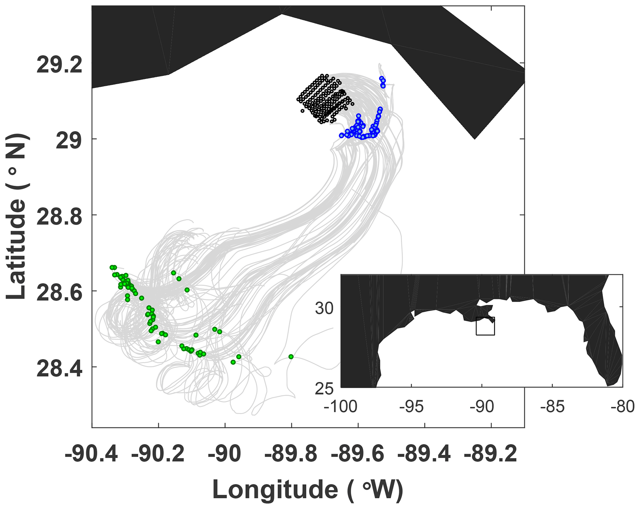
Figure 1 Trajectories of the SPLASH drifters, with their positions at the release time, 1 d, and 3 d shown by black, blue, and green dots, respectively. The inset shows the geographical location of the experiment site, with the black box indicating the domain shown in the main panel.

In this paper, seven commonly used dynamical systems techniques were applied to the real drifter dataset from the SPLASH experiment: finite-time Lyapunov exponents (FTLEs), trajectory path length, trajectory correlation dimension, encounter volume, Lagrangian-averaged vorticity deviation, dilation, and spectral clustering. The resulting real ocean LCSs were mapped and described, and, when possible, parallels were drawn between these observed structures and their more classical counterparts from textbook analytic or numeric examples. The seven techniques were also intercompared to each other, and the similarities/differences were discussed. Our choice of the seven techniques is by no means all inclusive and was inspired by Hadjighasem et al. (2017), who compared a similar selection of the dynamical systems methods (plus a few more and minus the encounter volume method) in the context of analytical, observed, and numerically generated flows.

2 Methods

We start with a brief review of the seven dynamical systems techniques that we will use.

2.1 FTLEs

One of the most commonly used LCS detection techniques is based upon FTLEs (Haller and Yuan, 2000; Shadden et al., 2005). The FTLE is the largest exponential separation rate between a trajectory and its closest neighbors in any direction. Maximizing ridges of FTLE fields can be used as proxies for stable (or unstable for backward-time trajectories) manifolds of hyperbolic trajectories in time-varying fluid flows (with the additional requirement that the fastest separation occurs in the direction normal to the ridge and is caused by the hyperbolic straining rather than shear). Regions with small FTLEs are indicative of slow separation rates between neighboring trajectories and often correspond to eddy cores. Maps of FTLEs are very visual, and the computation of FTLEs is straightforward, computationally inexpensive, and robust with respect to noise, which makes FTLEs one of the most popular methods in oceanographic studies of transport and mixing. Importantly, FTLEs are also frame-independent and thus give consistent results in any translating or rotating reference frame (Haller, 2005, 2015).

For flows where the velocity field is known from either models or observations, FTLEs (λ) can be estimated by releasing dense regularly spaced orthogonal grids of simulated trajectories (Haller, 2001, 2002). This method uses four (in 2D) closest neighbors to construct the Cauchy–Green tensor $G={\left(\frac{\mathrm{\Delta }{x}_i}{\mathrm{\Delta }{x}_{\mathrm{0},j}}\right)}^T\left(\frac{\mathrm{\Delta }{x}_i}{\mathrm{\Delta }{x}_{\mathrm{0},j}}\right)$, whose largest eigenvalue σ is connected to

$$\begin{array}{}\text{(1)}& \mathit{\lambda }={\displaystyle \frac{\mathrm{1}}{T}}\ln \surd \mathit{\sigma }.\end{array}$$

Here Δx_0,i and Δx_i are the initial and final distance in the ith direction between neighboring trajectories. This algorithm requires dense regularly spaced orthogonal grids of trajectories. For the SPLASH dataset, we manually chose quadruplets of four neighboring trajectories that form a near-rectangle, define the local orthogonal coordinate system most strongly aligned with the axes of the near-rectangle, and then estimate FTLEs using Eq. (1) for the center of mass of each quadruplet (Fig. 2 shows the quadruplets and their centers of mass locations).

Figure 2 Release locations of the SPLASH drifters (black dots) with the Delaunay delineation (grey lines) used to define the closest neighbors for estimating FTLEs at the drifter positions using the unstructured grid method. Grey circles show locations between the drifters, at which FTLEs were estimated via the structured grid method (using a quadruplet of black drifters around each grey dot).

A modification for unstructured meshes was described in Lekien and Ross (2010). Rypina et al. (2021) recently used the unstructured grid method to compute FTLEs from a cluster of six real drifters in the Alboran Sea. The method estimates FTLEs for each trajectory using its N closest neighbors as

$$\begin{array}{}\text{(2)}& \mathit{\lambda }={\displaystyle \frac{\mathrm{1}}{T}}\ln \stackrel{\mathrm{̃}}{\mathit{\sigma }},\end{array}$$

where $\stackrel{\mathrm{̃}}{\mathit{\sigma }}$ is the largest singular value of a matrix

$$\stackrel{\mathrm{̃}}{\mathbf{M}}={\mathbf{DX}}_{\mathrm{f}}{\left({\mathbf{DX}}_{\mathrm{0}}\right)}^T{\left({\mathbf{DX}}_{\mathrm{0}}{\left({\mathbf{DX}}_{\mathrm{0}}\right)}^T\right)}^{-\mathrm{1}},$$

which minimizes ∥DX_f−M DX₀∥.

Here,

$${\mathbf{DX}}_{\mathrm{0}}=\left(\begin{array}{ccc}{x}_{\mathrm{1}}^{\mathrm{0}}-x_i^{\mathrm{0}}& \mathrm{\dots }& x_N^{\mathrm{0}}-x_i^{\mathrm{0}}\\ y_{\mathrm{1}}^{\mathrm{0}}-y_i^{\mathrm{0}}& \mathrm{\dots }& y_N^{\mathrm{0}}-y_i^{\mathrm{0}}\end{array}\right)$$

and

$${\mathbf{DX}}_{\mathrm{f}}=\left(\begin{array}{ccc}{x}_{\mathrm{1}}^f-x_i^f& \mathrm{\dots }& x_N^f-x_i^f\\ y_{\mathrm{1}}^f-y_i^f& \mathrm{\dots }& y_N^f-y_i^f\end{array}\right)$$

are matrices of the initial and final displacements between the trajectory and its N neighbors. Because the largest singular value of $\stackrel{\mathrm{̃}}{\mathbf{M}}$ is equal to the square root of the largest eigenvalue of $\stackrel{\mathrm{̃}}{G}={\stackrel{\mathrm{̃}}{\mathbf{M}}}^T\stackrel{\mathrm{̃}}{\mathbf{M}}$, Eq. (2) is the unstructured-mesh counterpart of Eq. (1). We use the Delaunay triangulation partition to define closest neighbors for each drifter (Fig. 2 shows the Delaunay partition for the SPLASH dataset). The FTLE is then estimated using Eq. (2) at each drifter's initial position using its Delaunay closest neighbors. When used together, a combination of these two methods – the regular and the unstructured mesh methods – allows FTLEs to be estimated both at the locations of each drifter and between neighboring quadruplets.

2.2 Trajectory path length

Trajectory path length $L=\int \mathrm{d}s={\int }_{t_{\mathrm{0}}}^{t_{\mathrm{0}}+T}\mathrm{|}\mathit{u}\left(x\right(t),t)\mathrm{|}\mathrm{d}t$, where ds is the incremental length of the infinitesimal trajectory segments. For drifter data, summation can be used instead of integration. L has been proposed by Rypina et al. (2011) as one of the “trajectory complexity measures” and by Mendoza and Mancho (2010) as the “Lagrangian descriptor” for identifying LCSs. Curves of near-constant L values with a large ∇L in the perpendicular direction to the curve are indicative of the stable manifolds of hyperbolic trajectories (because trajectories on the manifold approach the hyperbolic trajectory, and trajectories slightly off the manifold are repelled from it). This method is less mathematically rigorous than FTLEs and frame dependence, but it is commonly used due to its simplicity.

2.3 Trajectory correlation dimension

The trajectory correlation dimension (CD) is a measure of space occupied by a trajectory. In 2D, it varies from 0 for a point to 1 for a curve to 2 for a trajectory that densely fills an area. C can be estimated using a box-counting algorithm, where the entire trajectory dataset is first mapped onto a unit square, and the unit square is then repeatedly split into 2^−2m, $m=\mathrm{0},\mathrm{1},\mathrm{\dots },M$ adjacent square boxes with side length $s={\mathrm{2}}^{-m}$ (we use M=12 in this paper). A distribution function is then computed for each trajectory as $F_i\left(s\right)=\frac{\mathrm{1}}{N_i^{\mathrm{2}}}\mathrm{\Sigma }\left(N_i^j\right(s){)}^{\mathrm{2}}$, where N_i is the total number of points in the ith trajectory, and $N_i^j$ is the number of points in the ith trajectory that fall inside the jth box for a given s. The trajectory correlation dimension CD_i for the ith trajectory can then be estimated as the slope of F_i(s) vs. s in log–log coordinates. Just like trajectory path length, CD is another measure of trajectory complexity and has been proposed by Rypina et al. (2011) as a means for LCS identification. Similar to L, level curves of near-constant CD values with a large ∇CD in the perpendicular direction to the curve are indicative of the stable manifolds of hyperbolic trajectories. CD is a more sensitive measure of trajectory complexity than L but is more computationally expensive. Just like L, the CD is also frame-dependent. Note also that for flows in the state of chaotic advection, the CD (and L) could also be used to highlight slowly moving coherent eddy-like features (regular islands), embedded into vigorously stirring regions (chaotic sea). Islands would have less complex trajectories with lower CD than trajectories within the chaotic sea. Similarly, although the CD was not designed to identify convergence, trajectories converging rapidly into a nearly stationary convergence zone would have a smaller CD than those free to wander over the entire domain.

2.4 Trajectory encounter number and trajectory encounter volume

The trajectory encounter volume V_en for a particular trajectory is a volume of fluid that gets in contact with a particular water parcel over a time interval T (Rypina and Pratt, 2017; Rypina et al., 2018). This is a frame-independent quantity. It quantifies the mixing potential of a flow and is related to the eddy or turbulent flow diffusivity κ (Rypina et al., 2018). The larger V_en is, the more opportunities exist for a parcel to exchange properties with surrounding fluid. The smallest V_en occurs in isolated secluded regions of the flow such as eddy cores, and the largest V_en occurs in hyperbolic regions and along the stable manifolds of hyperbolic trajectories leading into hyperbolic regions. Thus, V_en can be used to characterize both elliptic and hyperbolic LCSs.

For datasets containing a finite number of particle trajectories, the encounter volume for a particular trajectory can be approximated by assigning small volumes δV_j to all trajectories and summing over those trajectories that come close to the particular trajectory: $V_{\mathrm{en}}\approx \sum \mathit{\delta }{V}_j$. For regular grids $\mathit{\delta }{V}_j=\mathit{\delta }V=\mathrm{const}$ and V_en=δVN_en, where N_en is the encounter number – the number of trajectories that come close (i.e., within a small radius R) to the particular trajectory. In our calculations, we use R=1 km and δV≈1 km², which is the square of the mean distance between the drifters' release locations.

Note that the interpretation of the encounter volume in the context of limited trajectories deployed in a small part of a flow domain, such as our SPLASH drifters, differs from the case where drifters are seeded over the entire domain. Only for a domain-wide deployment is encounter volume representative of the mixing potential of the flow. For a small deployment, the encounter volume merely measures the amount of encounters within the dataset. This undersampling issue leads to important consequences in both hyperbolic and elliptic regions. While for a domain-wide deployment a lot of encounters occur in hyperbolic regions (as discussed above), these are also the exact same regions where initially nearby trajectories separate rapidly from each other, yielding low encounter values in the case of a small deployment. Similarly, whereas coherent eddy cores produce fewer encounters than hyperbolic regions for a domain-wide drifter release, these regions trap drifters, allowing them to encounter many of their neighbors deployed within the same eddy, which produces large values in the case of small deployment. Thus, the encounter volume might be a poor measure of the mixing potential of a flow in the case of a small deployment (but because this metric is still sensitive to differences between hyperbolic/elliptic behaviors even for a small deployment, it might still be able to highlight regions with different transport characteristics, so we go ahead and apply it to SPLASH drifters in the next section).

2.5 Dilation

The dilation rate (with units of inverse time) is the velocity divergence averaged along a particle's trajectory, $D=\frac{\mathrm{1}}{T}{\int }_{t_{\mathrm{0}}}^{t_{\mathrm{0}}+T}\mathrm{div}\left(\mathit{u}\right(x\left(t\right),t\left)\right)$. This frame-independent quantity was proposed by Huntley et al. (2015) as a method for identifying clusters of material at the ocean surface. We will refer to D simply as “dilation” for brevity. Trajectories with the largest positive/negative D experience the strongest divergence/convergence and thus repel/accumulate buoyant floating surface tracers (including drifters). D can be used to identify convergence-type LCSs marked by the extrema of D. For drifter data, summation can be used instead of integration, and the linear least-squares method of Molinari and Kirwan (1975) can be used to estimate div(u) at each point along each trajectory.

2.6 Lagrangian-averaged vorticity deviation (LAVD)

LAVD is the vorticity deviation with respect to the domain-averaged instantaneous vorticity, averaged along a particle trajectory, $\mathrm{LAVD}=\frac{\mathrm{1}}{T}{\int }_{t_{\mathrm{0}}}^{t_{\mathrm{0}}+T}\mathrm{|}\mathit{\omega }\left(x\right(x_{\mathrm{0}},t)-\stackrel{\mathrm{‾}}{\mathit{\omega }\left(t\right)}\mathrm{|}\mathrm{d}t$. It was introduced by Haller et al. (2016) as a frame-independent metric for identifying rotationally coherent Lagrangian eddies, which correspond to a region contained within the outermost closed convex level surface of LAVD surrounding an isolated maximum. For drifter data, we again use summation instead of integration and estimate vorticity using a linear least-squares method. Note that LAVD would only be able to identify those rotationally coherent Lagrangian eddies that are smaller than, and lay entirely within, the domain seeded with drifters.

2.7 Spectral clustering

The last method for identifying the LCSs that we will be testing using drifter data is the optimized-parameter spectral clustering described in Filippi et al. (2021a, b; see also Shi and Malik, 2000; Hadjighasem et al., 2016; and references therein). This was originally a data science technique that was adopted by the dynamical systems community. This method aims at identifying, within a given dataset of trajectories, clusters of trajectories that are most similar to each other and, at the same time, most dissimilar from trajectories in other clusters. A direct connection between spectral clusters and elliptic/hyperbolic/convergence-type LCSs from other methods is not always straightforward, although some of the identified spectral clusters often coincide with elliptic regions, regions of strong convergence, or regions delineated by segments of hyperbolic LCSs. The method starts with the construction of a matrix of weights

$${\mathbf{w}}_{ij}=\left\{\begin{array}{c}\frac{\mathrm{1}}{r_{ij}}\\ w_{\mathrm{diag}}\end{array}\right.,$$

where r_ij is the time-averaged distance between the ith and jth trajectories, and w_diag is a large constant offset value (we use $w_{\mathrm{diag}}=max\left(w_{ij}\right)\times {\mathrm{10}}^{\mathrm{7}}$). Based on this matrix, the method used ideas from machine learning theory, specifically N-cut matrix partitioning and K-means clustering algorithms, to identify the spectral clusters with the largest/smallest degree of intra-/inter-cluster similarity. Importantly, the optimized-parameter version of the spectral clustering method (Filippi et al., 2021a, b) that we are using automatically detects both the optimal number of clusters and the cluster sizes (based on the normalized eigengap between the eigenvalues of the generalized normalized Laplacian, as described in Filippi et al., 2021a). Being based on the distances between trajectories, spectral clustering is frame-independent.

2.8 Linear least-squares (LLS) method for estimating drifter-based divergence and vorticity

In order to estimate divergence and vorticity from drifters, we follow the approach of Rypina et al. (2021), where we first compute horizontal velocities from drifter positions using a centered finite-difference scheme and then apply the linear least-squares (LLS) method of Molinari and Kirwan (1975) to estimate horizontal velocity gradients. The LLS method is based on the Taylor expansion of velocity, U=DA, where $\mathit{U}={\left[u_{\mathrm{1}},\mathrm{\dots }{u}_N\right]}^T$ is a (known) vector containing the u velocity at a given time t for each of the N drifters,

$$\mathbf{D}=\left(\begin{array}{ccc}\mathrm{1}& x_{\mathrm{1}}-\stackrel{\mathrm{‾}}{x}& y_{\mathrm{1}}-\stackrel{\mathrm{‾}}{y}\\ \mathrm{⋮}& \mathrm{⋮}& \mathrm{⋮}\\ \mathrm{1}& x_N-\stackrel{\mathrm{‾}}{x}& y_N-\stackrel{\mathrm{‾}}{y}\end{array}\right)$$

is a known distance matrix containing instantaneous distances from each drifter to the center of mass of the drifter distribution at time t, and $\mathit{A}={\left[\stackrel{\mathrm{‾}}{u},\frac{\partial u}{\partial x},\frac{\partial u}{\partial y}\right]}^T$ is the vector containing the unknown velocity derivatives at time t that can be estimated using the Moore–Penrose pseudo-inverse as $\mathit{A}={\left({\mathbf{D}}^T\mathbf{D}\right)}^{-\mathrm{1}}{\mathbf{D}}^T\mathit{U}$ (and similarly for the v component).

Note that methods other than LLS can also be used to compute divergence and vorticity. Specifically, divergence can be estimated as a rate of change of the area spanned by the drifter polygon, and both divergence and vorticity can be estimated using Green's theorem as, respectively, the circulation around and total flux through the drifter polygon. Rypina et al. (2021) compared all three techniques in detail using both real and simulated drifters deployed in the Alboran Sea at similar inter-drifter distances as the SPLASH drifters and observed good correspondence between all three techniques for clusters of six drifters, as long as the drifters stayed within a few kilometers of each other and the aspect ratio was reasonably small (≤ 5). For larger aspect ratios, all methods started to deteriorate. Essink et al. (2022) also investigated the optimal way of computing velocity gradients, divergence, and vorticity from drifters. By quantifying the uncertainty in the velocity gradient calculation for different methods and different drifter configurations in a high-resolution submesoscale-resolving ocean circulation model, they concluded that the LLS was the most robust among the three methods and that the accuracy of the LLS estimates grew linearly with the increasing number of drifters and decreased logarithmically with the increasing aspect ratio of the drifter polygon (i.e., LLS works best for tight equidistant polygons with many drifters). Based on their analysis, they favored LLS over the area rate of change and Green's theorem methods as their preferred method and proposed six drifters with a polygon length scale of about 10 km and an aspect ratio of less than 10 as an optimal parameter range for reliable estimation of velocity gradients. They then successfully used LLS with these parameter criteria for estimating divergence and vorticity from the drifters in the Bay of Bengal.

Guided by recommendations of Rypina et al. (2021) and Essink et al. (2022), in this paper we will rely on the LLS method for estimating velocity gradients and will refer to the LLS estimates of divergence and vorticity as trustworthy (and mark them by colored circles) if there are ≥ six drifters within a 3 km radius, the center of mass of the drifter distribution is located within the polygon, and the polygon aspect ratio is ≤ 6. If only the aspect ratio condition is not satisfied (but the number of drifters, the distance, and the center of mass conditions are), we will still compute LLS estimates, but we will refer to them as less trustworthy (and mark them by colored diamonds). In all other cases, we do not produce estimates of divergence and vorticity.

3 Results

We start by qualitatively separating the motion of drifters into three stages. For about a day after deployment, all drifters started moving together in an anticyclonic fashion to the north and then northeast towards the coast (Fig. 1) – this is what we will refer to as the initial stage of motion. Upon approaching the shelf, the drifters halted their onshore motion and split into two groups, a smaller northern group that headed northward along the coast and a larger southern group that moved southward. This splitting behavior was reminiscent of a hyperbolic motion in the vicinity of a hyperbolic trajectory, with a stable manifold emanating from a hyperbolic trajectory in the offshore direction and two unstable manifolds northward and southward from it in the along-shore direction. As a result, a long and narrow filament roughly aligned with the coast is quickly formed just after 1 d. This filament contains about one-third of all the drifters, with the rest of the drifters forming a less elongated and more compact blob just south-southwest of the filament. Some clustering temporarily occurs at about 1 d near the southeastern corner of the drifter configuration but goes away later. The slowdown of the onshore movement, the splitting into the north–south groups, and the formation of the elongated along-shore filament constitute the second stage of motion, which lasted from about 0.9 to about 1.25 d after the deployment. Finally, during the third stage of motion, the drifters started moving offshore to the southwest. As they progress further from the coast, trajectories started exhibiting more looping and the drifters dispersed further apart from one another, although they still remained in an elongated filament configuration (not anymore aligned with the coast) all the way until day 5, which is the end time of this dataset.

Having split the drifter movement into three stages, we next apply our Lagrangian methods to trajectory segments from t_start = 0 d until t_end = 0.5, 1, and 3 d, respectively (top, middle, and bottom row of panels in Figs. 3–9). The resulting fields highlight the dominant LCSs that existed at the time of the drifter deployment (i.e., at t_start = 0) and that governed the movement of drifters during the subsequent 0.5, 1, and 3 d, respectively. Since all seven identifiers map out LCSs at the start time of trajectory, using t_start = 0 allowed us to make the best use of the nearly regular deployment pattern. Fields computed for other time intervals, for example, [0.5, 1] d or [1, 3] d, would need to be mapped to the location of trajectories at 0.5 and 1 d, respectively, when drifters already stretched into highly elongated filaments, thus losing the advantage of the regular deployment grid.

Figure 3 Real-drifter-based FTLEs at (a–c) 0.5 d, (d–f) 1 d, and (g–i) 3 d, mapped to the initial (a, d, g) and current (b, e, h and c, f, i) positions of the drifters.

FTLEs (Fig. 3). During the initial stage of motion (t_start = 0 d and t_end = 0.5 d), the FTLE field did not show any clear coherent structures, neither hyperbolic (maximizing ridges) nor elliptic (isolated regions with significantly lower FTLEs). During the intermediate stage (t_start = 0 d and t_end = 1 d), the largest FTLEs were observed along the northwestern edge of the release domain, containing drifters that split north–south upon approaching the coast and formed an elongated along-shelf filament. FTLEs were negative for drifters released near the middle of the northeastern edge of the release domain, which converged into a tight cluster in the southeastern corner of the drifter distribution at 1 d. This feature was transient and disappeared as the drifters moved offshore. The rest of the release domain has small positive FTLE values; these were the drifters which did not experience strong along-shore alignment and formed a more compact group in the southern part of the drifter distribution at 1 d. Finally, during the third stage of motion (t_start = 0 d and t_end = 3 d), as the drifters moved offshore and reshaped into a northwest–southeast configuration, the only distinguishing feature of the FTLE field was the blue cluster near the central part of the release domain. This cluster contained trajectories that either remained together or separated and then came back together (since some of these data points are marked by yellow in the top row). When mapped to the current positions of the drifters at 3 d, these smallest blue FTLEs corresponded to a group of drifters in the western part of the distribution, i.e., a cluster of blue dots in the lower middle and right panels of Fig. 4. (Note that the northwest–southeast configuration at 3 d was mostly formed from the drifters located in the southern part of the distribution at 1 d and so is different from the along-shelf “tail”.)

To summarize, although no clear coherent sets were distinguishable at early stage, the characteristic patterns became clearer at later stages. Largest FTLEs indicated regions of strong drifter separation that, during the intermediate stage of motion, were reminiscent of stable manifolds of hyperbolic trajectories. Smallest FTLEs highlighted groups of drifters that stayed closer together compared to their neighbors. Transient negative FTLE regions were also present and highlighted groups of drifters temporarily converging into tight clusters (before spreading apart again later on). The FTLEs varied significantly with the increasing duration of trajectories, i.e., increasing t_end, suggesting that different flow features governed the movement of drifters during different stages of motion. The calculation of FTLEs was straightforward and computationally inexpensive, and by combining the structured and unstructured grid methods, we were able to obtain FTLE values at both drifter release positions and in between them, providing twice higher resolution compared to other methods.

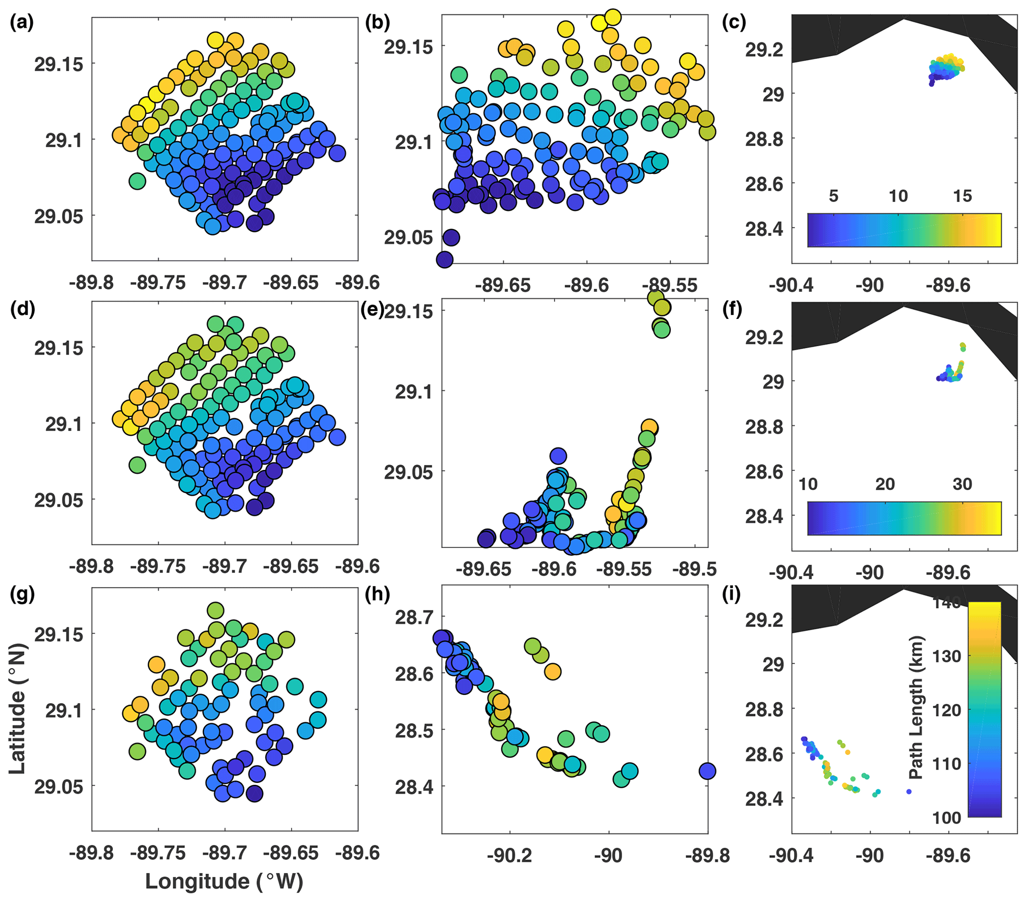
Figure 4 Real-drifter-based path length at (a–c) 0.5 d, (d–f) 1 d, and (g–i) 3 d, mapped to the initial (a, d, g) and current (b, e, h and c, f, i) positions of drifters.

L (Fig. 4). Trajectory path length L showed an increase in values with increasing latitude across the release domain at all times, with the largest/smallest values in the northwest/southeast. This large-scale gradient in L was dominated by the faster anticyclonic motion of the northwestern drifters at early times. This was reminiscent of a solid body rotation, where the northwestern drifters that were located further from the center of rotation than their southeastern neighbors moved at a faster speed and thus covered a longer path length over a given time interval. (This effect could presumably be removed by recalculation of L in an appropriate rotating frame of reference, an operation that would not change the values of the FTLEs. Thus it is perhaps not surprising that the distributions of the two metrics differ in significant ways.) All other characteristic features, such as the splitting of trajectories into the northern and southern group at about 1 d, the formation of an elongated along-shelf filament, the transient convergence region, and the reshaping of the drifter configuration as it progressed further offshore, had only minor effects on the resulting path length fields. Specifically, we tried looking for hyperbolic LCSs, which would show up as level sets of L with the highest gradient in the perpendicular direction, and for slow-moving elliptic regular regions, which should be characterized by a uniformly low L with a high gradient toward large L at the periphery, but we did not find any. Thus, despite being easy to compute and straightforward to interpret, the path length L was only marginally useful in identifying the dominant LCSs.

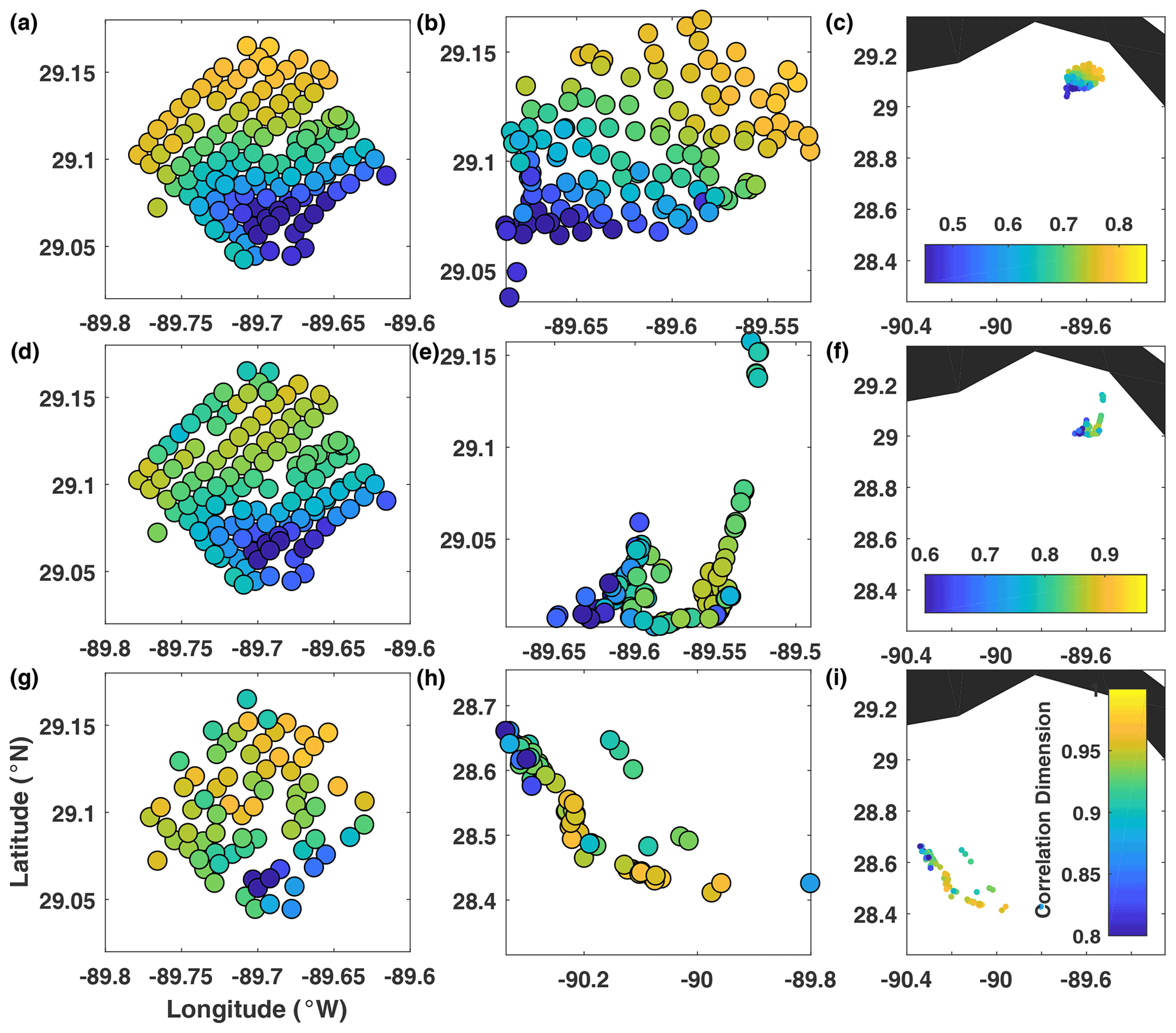
Figure 5 Real-drifter-based correlation dimension at (a–c) 0.5 d, (d–f) 1 d, and (g–i) 3 d, mapped to the initial (a, d, g) and current (b, e, h and c, f, i) positions of drifters.

CD (Fig. 5). Results for the trajectory correlation dimension CD were generally similar to those for the trajectory path length, in that CD was also dominated by the across-domain gradient from northwest to southeast, and the distribution of CD did not change dramatically in time. Although CD is a more sensitive, and also more computationally expensive, measure of trajectory complexity, it was still not able to identify the LCSs responsible for either the formation of the elongated filament at 1 d or the transient convergence zones just after 1 d or the suppressed separation between trajectories coming from the central part of the domain at 3 d. Overall, CD was no more useful than L in identifying the LCSs and, like L, had the same frame dependence issues.

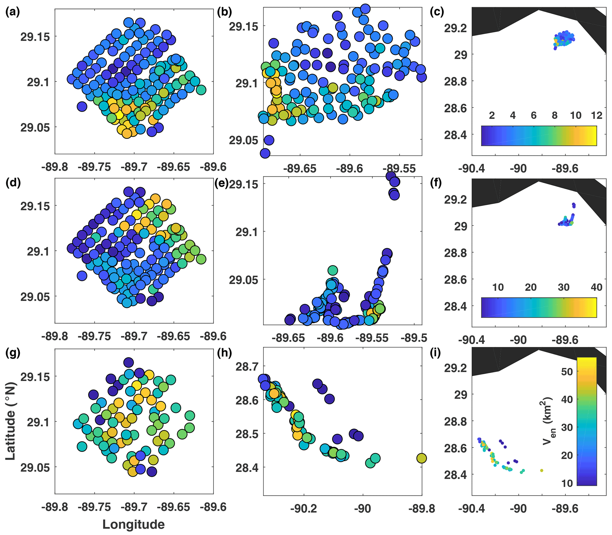
Figure 6 Real-drifter-based encounter volume at (a–c) 0.5 d, (d–f) 1 d, and (g–i) 3 d, mapped to the initial (a, d, g) and current (b, e, h and c, f, i) positions of drifters.

V_en (Fig. 6). The encounter volume V_en was able to successfully highlight several different flow features governing the movement of drifters at different stages of motion. During the initial stage, V_en had the largest values in the southern part of the release domain. From the top middle panel (the map of V_en at the current position of the drifters), we observed that these enhanced values were caused by the tighter clustering of drifters (so that they were able to meet more neighbors). During the intermediate stage of motion, the distribution of V_en changed, and the largest values migrated to the northeastern edge of the release domain. This was associated with the transient convergence zone (that we also observed in the FTLE fields); trajectories released in that area converged into a tight cluster located at the southeastern corner of the drifter distribution at 1 d (second row, middle panel). The elongated along-shore filament seen at 1 d contained the smallest V_en since trajectories in the filament separated rapidly from their nearby neighbors and thus did not encounter many SPLASH trajectories. This is likely a consequence of undersampling in hyperbolic regions (note that the same region was marked by largest FTLEs indicative of hyperbolic behavior). Since SPLASH drifters were only seeded over a small O(10 km²) domain, the resulting V_en characterizes encounters within this limited dataset, rather than with all trajectories in the entire domain, leading to smallest V_en in this hyperbolic region instead of largest V_en, as would likely have been the case for a domain-wide trajectory deployment. Trajectories that headed north after approaching the coast at 1 d never caught up with the rest of the distribution, always staying behind, i.e., to the north from the rest of the drifters. Thus, these drifters experienced the least number of encounters and, during the third stage of motion, had the smallest V_en values. Apart from this low-encounter-number group, there were no other pronounced features in the V_en field during the third stage of motion.

It is interesting to compare and contrast V_en with FTLEs, which became sort of a benchmark for the LCS detection problems, being frame-independent, commonly used, and easy to compute. There are significant differences between the distributions of the two metrics, reflecting differences in what the two are actually measuring. While both FTLEs and V_en are sensitive to flow convergence/divergence, trajectory clustering, and hyperbolic behavior, one of the key differences between them is that V_en is a time-integrated measure that depends on the behavior of trajectories over the entire time interval between the initial and final times, whereas FTLEs only depend on the initial and final positions of drifters (i.e., FTLEs do not care how trajectories got to their final positions, whereas V_en does). For example, even though trajectories comprising the low-FTLE blue cluster in the western part of the distribution at 3 d have come close together at that time, over a time frame of 3 d they experienced no more trajectory encounters than many other trajectories outside of that blue FTLE cluster (and thus were not standing out in the V_en field). V_en is also more susceptible to undersampling issues than FTLEs, since the number of encounters within a limited dataset is not necessarily representative of that with trajectories seeded over the entire domain. For SPLASH drifters, undersampling led to smallest V_en along the northwestern edge of the release domain during the second stage of motion, where large FTLEs indicated the presence of a stable manifold of a hyperbolic trajectory that was responsible for the formation of an elongated along-shore filament at 1 d.

Overall, despite some challenges with undersampling, the encounter volume V_en proved to be an interesting frame-independent diagnostic that was sensitive to both enhanced clustering, hyperbolic behavior, and flow convergence, and was complementary to FTLEs.

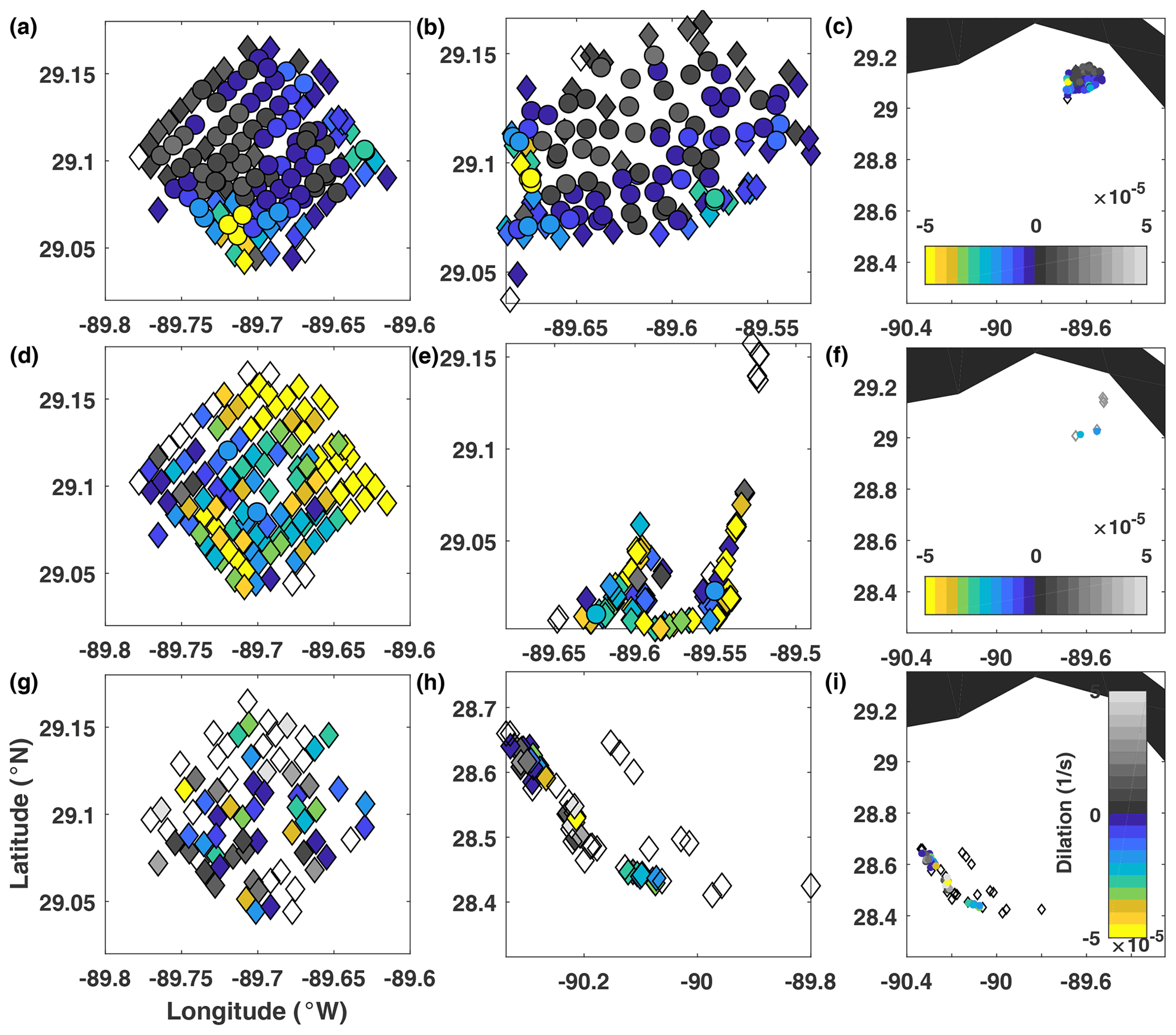
Figure 7 Real-drifter-based dilation at (a–c) 0.5 d, (d–f) 1 d, and (g–i) 3 d, mapped to the initial (a, d, g) and current (b, e, h and c, f, i) positions of drifters. Colored circles, colored diamonds, and empty (white) diamonds mark drifters for which calculation of gradients was most reliable, less reliable, and not reliable, respectively, according to the LLS reliability criteria described in the Methods section.

D (Fig. 7). The challenge with computing dilation D (as well as LAVD) for real drifters is the inability to reliably estimate divergence (vorticity) for isolated drifters and drifters forming strongly elongated polygons. This was not a problem for SPLASH drifters during the early stage of motion but became an issue as the drifters started to spread apart and formed elongated filaments. During the initial stage of motion (top row), the most pronounced feature of the D field was the negative cluster in the southern corner of the release domain, which contained drifters that converged more than their neighbors. A similar feature has been identified by V_en as the high-encounter-volume region. The rest of the domain had near-zero dilation. During the second stage of motion (middle row), the negative dilation in the south diminished, and another convergent negative-D region appeared along the northeastern edge and eastern corner of the release domain. This is reminiscent of the negative-FTLE and high-V_en region in the middle rows of Figs. 3 and 6. Trajectories released there converged into the southeastern corner of the drifter distribution at 1 d. Around this time, an increasing number of trajectories started having unreliable divergence values; for example, divergence, and thus dilation, could not anymore be reliably computed for the northern group of trajectories, which became too few and too sparse. During the third stage of motion, this problem became even more important, and by day 3, the dilation field was undefined for about half of the trajectories. The resulting D field was noisy and did not exhibit any pronounced features.

Overall, dilation D was useful in highlighting the convergence zones during the first two stages of motion, but numerical difficulties associated with reliably estimating divergence for sparse datasets and elongated drifter configurations made it challenging to compute D over long time intervals from real drifters.

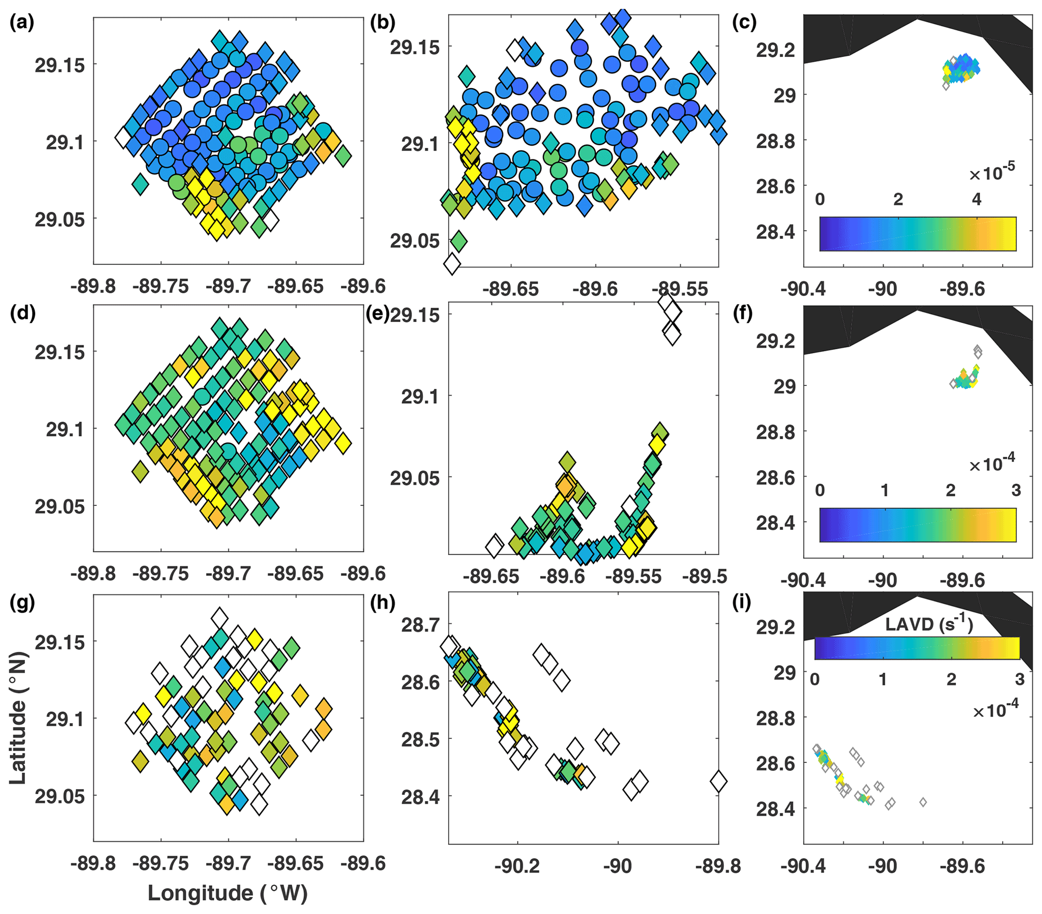
Figure 8 Real-drifter-based LAVD at (a–c) 0.5 d, (d–f) 1 d, and (g–i) 3 d, mapped to the initial (a, d, g) and current (b, e, h and c, f, i) positions of drifters. Colored circles, colored diamonds, and empty (white) diamonds mark drifters for which calculation of gradients was most reliable, less reliable, and not reliable, respectively, according to the LLS reliability criteria described in the Methods section.

LAVD (Fig. 8). During the first stage of motion, the strongest feature in the LAVD map was the yellow large-LAVD region near the southern corner of the release domain. This area coincided roughly with the negative-D and large-V_en regions in Figs. 6–7. During the second stage of motion, this feature diminished in intensity, and a second high-LAVD region appeared near the eastern corner of the domain. Again, a similar region has been highlighted by low FTLEs, high V_en, and negative D, although LAVD emphasized the eastern corner rather than the entire northeastern edge of the release domain. Trajectories starting there converged into a tight cluster near the southeastern corner of the drifter distribution at 1 d. It is interesting that LAVD identified similar regions as FTLEs, V_en, and D, despite the fact that clustering behavior and flow convergence do not necessarily need to be associated with increased vorticity deviation. In our case, clustering and convergence did coincide with increased vorticity deviation, suggesting that perhaps a small-scale eddy or recirculation that was affecting this particular cluster of drifters might have been responsible for all of these effects. (Note that interpreting the vorticity deviation as vorticity is only possible when the domain-averaged background vorticity, $\stackrel{\mathrm{‾}}{\mathit{\omega }}$, is small, which was not always the case for the SPLASH drifters.) Finally, during the third stage of motion (bottom row), the map of LAVD became gappy (because, similar to the challenges with dilation, here we could not reliably estimate LAVD for about half of the drifters) and showed no distinguished regions. However, when mapped to the current position of the drifters (lower middle panel), the cluster in the middle of the drifter distribution showed larger LAVD values than clusters to the northwest and southeast (but since trajectories forming the middle cluster came from different parts of the release domain, this feature did not stand out in the left panel).

Overall, during the first two stages of motion, LAVD highlighted two regions with enhanced LAVD values. While large LAVD does not generally indicate convergence, in our case both regions were strongly convergent. At later times, vorticity estimation became less reliable, and it became harder to distinguish coherent features in the sparse and noisy map of LAVD. Note that our high-LAVD regions differed from the classical examples of rotationally coherent Lagrangian eddies. Our regions were not circular, did not have a single maximum, and were too noisy to identify the outermost convex contour level, which marks the outer edge of the coherent rotational eddies in the standard application of the LAVD technique. Thus we cannot call these high-LAVD features rotationally coherent Lagrangian eddies. It is interesting that even though trajectories exhibited clear anticyclonic rotation during the first 12 h, LAVD did not identify this anticyclonic eddy. We think this might be because the SPLASH release domain was too small and was located entirely within this vortex structure.

Figure 9 Real-drifter-based spectral clusters at (a–c) 0.5 d, (d–f) 1 d, and (g–i) 3 d, mapped to the initial (a, d, g) and current (b, e, h and c, f, i) positions of drifters.

Spectral clustering (Fig. 9). At early times, the number of coherent clusters identified by the SC algorithm was quite large (12), although some clusters only contained a few drifters. (Recall that the optimized-parameter SC is able to autonomously identify the optimal number and optimal size of the clusters, without input from the user). Among the detected clusters, the yellow cluster located in the south-southwest of the release domain is perhaps the most noteworthy because it resembled the low-FTLE, large-V_en, negative-D, and large-LAVD region that contained trajectories that stayed close together during the initial stage of motion. As the drifters entered the second stage of motion, the number of identified coherent clusters decreased to six. Most of the release domain was split between two large clusters – the cyan cluster in the north-northeast containing drifters attracted by the convergence region (i.e., drifters that converged/came close to the southeastern corner of the drifter distribution at 1 d) and the green cluster in the south of the release domain containing drifters that did not feel the pull of that convergence zone. The remainder of the domain, i.e., the northwestern edge of the domain that mostly contained the trajectories forming an elongated along-shore filament, was split into four more clusters. Finally, at the third stage of motion, the drifters were split into eight clusters, and the grouping was most straightforward to interpret by looking at the lower middle panel. All trajectories in the western cluster were blue (these trajectories came from the central and southern portion of the domain in the bottom left panel), with the orange cluster to the southeast of it (these trajectories came from around the periphery of the blue cluster in the bottom left panel) and with the red group further to the southeast of the orange cluster (most red trajectories originate from the northeastern edge of the release domain in the bottom left panel). The remaining five clusters only contained one or two trajectories.

Overall, the spectral clustering algorithm seems to have identified physically meaningful and intuitively clear coherent clusters; the movement was similar for drifters within each cluster and dissimilar between the clusters. There were also good correspondences between the spectral clusters and coherent featured highlighted by other methods.

4 Summary and discussion

SPLASH drifter experiment provided the long-awaited opportunity to test the performance of different dynamical systems techniques with real, rather than simulated, ocean drifters. Although many other drifter datasets are available for various regions of the World Ocean, drifters are typically released by a handful here and there, and the resulting data are typically inadequate for mapping out the LCSs. For example, NOAA's Global Drifter Program dataset contains several thousands of near-surface drifter trajectories released between 1971 and today, but the density of the drifter distribution at any given time is only about one per 5^∘ × 5^∘ box, which is too sparse to identify even mesoscale LCSs.

Three qualitatively different stages of motion were evident in the SPLASH drifter data. During the first stage, all drifters moved anticyclonically toward the coast. During the second stage, the drifters halted their onshore motion, split north–south, and formed an elongated along-shelf filament. During the third stage, the drifters moved offshore, rearranging themselves into a northwest–southeast configuration. As the character of drifter movement changed with time, the maps of the Lagrangian metrics and the resulting LCSs that they highlighted changed as well. In order to capture this time dependence, we have applied the Lagrangian metrics to segments of trajectories from fixed t_start = 0 d to variable t_end = 0.5, 1, and 3 d. When the Lagrangian metrics were mapped back to the initial positions of drifters at t_start, the resulting maps highlighted the dominant LCSs (such as the hyperbolic-type LCS responsible for the formation of the along-shore filament at 1 d, the convergence-type LCS attracting drifters into the southeastern corner at 1 d, and the elliptic-type LCS forming during the 3rd stage of offshore motion) which existed at the time of the deployment within the deployment domain and which govern the subsequent motion of drifters over the corresponding time interval. The fact that the results for any particular measure differed between the three time intervals is consistent with submesoscale dynamics, where fronts, small eddies, and filaments form, evolve, and disappear on timescales of days or less.

The Lagrangian techniques we have examined include FTLEs, trajectory path length, trajectory correlation dimension, trajectory encounter number, dilation, LAVD, and optimized-parameter spectral clustering. This list was motivated by Hadjighasem et al. (2017) and is by no means exhaustive, but it includes a variety of commonly used methods that are based on different properties of trajectories, make use of the different definitions of coherence, and thus aim to identify different types of LCSs. Interestingly, despite the differences in their underlying principles and methodologies, many of these methods identified similar features within the SPLASH drifter dataset.

Among the most prominent features that were highlighted by multiple methods were (1) the region near the northwestern edge of the release domain (large FTLEs, small V_en, yellow/orange clusters), which contained trajectories that split north–south upon approaching the shelf and formed an elongated along-shelf filament at about 1 d; (2) the very strong but transient convergence region located near the northeastern edge of the release domain (negative FTLEs, large V_en, strongly negative dilation, cyan spectral cluster), which contained trajectories that converged into a tight cluster at about 1 d; and (3) the region in the central/southern part of the release domain (small FTLEs, blue spectral cluster), which contained trajectories that remained close to each other starting from 2.5 d and onward.

Although all of the identified structures were noisier and more complex than the classical elliptic and hyperbolic LCSs in textbook examples, some of the features bore resemblance to their classical counterparts. For example, the north–south splitting of trajectories starting within the yellow FTLE region near the northwestern edge of the domain was qualitatively similar to the behavior of trajectories near a hyperbolic region, where particles approach the hyperbolic trajectory along a stable manifold and then split and move away from the hyperbolic trajectory along the two unstable directions. The detected large-FTLE region near the northwestern edge of the release domain might thus possibly indicate the presence of a stable manifold in this region.

From the standpoint of numerical efficiency, FTLEs and L were the least computationally expensive, whereas CD, V_en, and spectral clustering were the most computationally expensive. However, with only 144 trajectories, the differences in the amount of time required to apply each technique were not critical. More importantly, FTLEs had the advantage of providing values at the positions of each drifter as well as between the neighboring drifters, effectively yielding output fields with twice the resolution of the other methods. FTLEs were also less affected by the gaps in GPS transmissions along trajectories because the estimation of FTLEs at a particular time only required knowing the initial and the current positions of the drifters, rather than requiring the information about the entire trajectory up to that time, as in the case of all other methods – path length, correlation dimension, encounter number, dilation, LAVD, and spectral clusters.

One challenge with dilation and LAVD is the loss of accuracy at longer times, when the drifters form elongated polygons. The deterioration of the velocity gradients estimates (that are required for estimating dilation and LAVD) with the increasing aspect ratio of the drifter polygon is intuitively clear. As the polygon elongates, the information about the velocity gradient in the perpendicular direction diminishes and is lost when the polygon approaches a one-dimensional line. This is true for all methods of velocity gradient estimation, not just for LLS, and presents a fundamental challenge for estimating dilation and LAVD from drifters, which tend to naturally form elongated filaments in oceanic flows.

It is interesting to note that the two frame-dependent methods – L and CD, which were dominated by the large-scale gradient across the entire release domain and did not highlight any submesoscale features – were the least useful in identifying LCSs. For SPLASH drifters, this dominant large-scale gradient developed during the initial anticyclonic phase of motion, when drifters deployed closer/further from the center of rotation were shorter/longer and less/more complex. This overpowering trend could potentially be removed by moving into a co-rotating reference frame (i.e., a natural frame of reference), but identifying such a natural reference frame is nontrivial in the absence of additional information about the flow.

Massive drifter releases such as SPLASH are extremely useful for improving our understanding of the transport and exchange processes at submesoscale. Specifically, data from the SPLASH and other similar experiments have been used for estimating diffusivity and studying particle spreading regimes at submesoscale (Poje et al., 2014; Beron-Vera and LaCasce, 2016). We have shown that a simultaneous release of about 100 drifters provides a glimpse of the dominant Lagrangian coherent structures that govern the transport of water and the movement of drifters.

The SPLASH experiment was not specifically focused on identifying LCSs, so the drifter release locations and timings were not optimized for capturing the underlying LCSs. Our analysis suggested that, luckily, a stable manifold of a hyperbolic trajectory was likely present in the northwestern edge of the domain spanned by the drifters at the time of their release and persisted for at least the first 1–1.5 d of the experiment. As explained above, this feature manifested itself as a high-FTLE region and was characterized by the north–south splitting of trajectories around day 1. However, no clear elliptic LCSs (i.e., coherent eddy cores) were identified by any of the methods, even though an anticyclone was likely present near the SPLASH release site at the time of deployment (based on the clockwise movement of drifters during the first day after release and on the numerical model simulations described in the Supplement). Note that even the LAVD method, which was specifically designed to identify rotationally coherent Lagrangian eddies, was also not able to highlight this anticyclone, possibly because LAVD is a wrong tool for identifying an eddy from a small trajectory set located entirely within an eddy. It is also possible that this anticyclone did not possess a Lagrangian core, or the core was located outside of the drifter release domain and/or was not properly resolved by the SPLASH drifters.

In the future, it would be interesting to repeat the experiment with the drifter deployment site and the release pattern optimized for capturing specific LCSs, whose presence could have been predicted based on a model or satellite data.

The very rapid nature of evolution at submesoscales may cause an evenly spaced array of drifters to rapidly collect into filaments, making it difficult to continue to accurately compute certain Lagrangian measures. In the SPLASH experiment, for example, the nearly rectangular deployment mesh of drifters (which took quite a bit of effort to achieve) eroded into an elongated filament over a timescale of about a day. Note, however, that it is precisely this rapid filamentation process and the rapid deformation of the initial mesh that give rise to the strong, pronounced, and detectable LCSs. A related challenge that complicates the understanding of the flow from the Lagrangian analysis presented here is that the features that are found (for example, a hyperbolic region) say something about local kinematic features of the flow but do not allow one to say much about what the flow looks like on broader spatial scales or over timescales longer than just a few days. The rapid filamentation experienced by the drifters prevents mapping out the structures at later times and over regions other than the original deployment domain. This might be one of the important things that we have learned about the flow and about sampling through massive drifter releases.

Finally, in order to investigate the reliability of the real-drifter-derived LCSs, we have simulated the SPLASH drifter dataset in a model and then compared the resulting SPLASH-like drifter-based LCSs to those computed using dense regular orthogonal grids of trajectories (we refer to the latter as dense-grid simulations). The results of these numerical simulations can be found in the Supplement. We used the operational data-assimilative Navy Coastal Ocean Model (NCOM) forecasting model for this purpose (https://doi.org/10.7266/n7-80ay-rx31; Jacobs and Spence, 2019).

Comparison between SPLASH-like and dense-grid model simulations showed reasonably good agreement for many, although not all, metrics and times, suggesting that many, although not all, SPLASH fields were reliable (see the Supplement). Specifically, SPLASH-like FTLEs were most reliable at shorter times and still meaningful at longer times in regions with strong hyperbolic-type LCSs located far enough away from each other to be resolved by the deployment grid. L and CD were reliable at all times, but since they did not identify any hyperbolic, elliptic, or convergence-type LCSs for SPLASH drifters, they were perhaps least useful among the seven methods. In contrast to FTLEs, V_en was not reliable at short times but improved its reliability at longer times. D and LAVD worked well at short times when drifters were still relatively close and did not form elongated filaments but deteriorated at longer times due to the rapid filamentation of the drifter distribution. Finally, SPLASH-like and dense-grid SC both identified large numbers of clusters within the SPLASH domain at short times and fewer clusters at longer times. At short time, the clusters were different between the SPLASH-like and dense-grid simulations; at longer times, there was a number of similarities in the identified clusters (longitudinal split along same longitude at an intermediate stage and assignment of most of the domain to 1 cluster at a later stage), but the details of the cluster configurations were different, especially near the edges of the domain.

Comparing observations to simulations, Lagrangian metrics were of similar magnitude for the real and simulated SPLASH drifter. The actual range of values in simulations and observations matched for FTLEs and D, as well as for L and CD at 0.5 and 3 d and for V_en at 0.5 d. LAVD was 2 to 3 times larger in observations, V_en was 2 to 3 times larger in simulations at the intermediate and late stages, and L and CD were slightly larger in simulations at the intermediate stage (note, however, that we used different times, specifically 1 d and 2 d, as a characteristic time for the intermediate stage in observations and simulations, respectively). Hyperbolic- and convergence-type LCSs were present in both observations and simulations, and no clear elliptic-type LCSs were seen in either model or observations. The model fields were generally significantly less noisy, exhibited a larger degree of coherence, and at early times had more positive dilation, compared to mostly near-zero and negative in observations. Detailed comparisons can be found in the Supplement.