Applying prior correlations for ensemble-based spatial localization

Localization is an essential technique for ensemble-based data assimilations (DAs) to reduce sampling errors due to limited ensembles. Unlike traditional distance-dependent localization, the correlation cutoff method (Yoshida and Kalnay, 2018; Yoshida, 2019) tends to localize the observation impacts based on their background error correlations. This method was initially proposed as a variable localization strategy for coupled systems, but it can also can be utilized extensively as a spatial localization. This study introduced and examined the feasibility of the correlation cutoff method as an alternative spatial localization with the local ensemble transform Kalman filter (LETKF) preliminary on the Lorenz (1996) model. We compared the accuracy of the distance-dependent and correlation-dependent localizations and extensively explored the potential of the hybrid localization strategies. Our results suggest that the correlation cutoff method can deliver comparable analysis to the traditional localization more efficiently and with a faster DA spin-up. These benefits would become even more pronounced under a more complicated model, especially when the ensemble and observation sizes are reduced.

1 Introduction

The ensemble Kalman filter (EnKF) is widely employed in modern numerical weather prediction (NWP) for refining the initial conditions of models and improving forecasts (Evensen, 2003). One of the notable features of EnKF is its flow-dependent background error covariance derived from the background ensembles (e.g., forecasts initialized at the last analysis time), which involves the time-evolving error statistics for the model state. The implied background error covariance together with the observation error covariance determine how much observation information should be used to generate a new analysis. Therefore, the accuracy of the background error covariance estimates is one of the most critical keys toward an optimal analysis for EnKF.

Houtekamer and Mitchell (1998) noticed that the background error covariance estimated by too few ensembles would introduce spurious error correlations in the assimilation. Incorrect error correlations are harmful to the analysis and could lead to a filter divergence. Hamill et al. (2001) performed conceptual experiments demonstrating how existing noises in the background error covariance influence the EnKF analysis. Their results showed that the relative error, also known as the noise-to-signal ratio, significantly increases when the ensemble size is reduced, and a large relative error would consequently degrade the analysis accuracy. These early studies concluded that a sufficient ensemble size is essential for EnKF to obtain reliable background error estimates and generate an accurate analysis. However, having large ensembles is computationally expensive, especially for high-resolution models. Hence, finding a balance between accuracy and computational cost becomes an inevitable challenge for modern EnKF applications. Recent EnKF studies usually limit their ensemble size to about 100 members, and the ensemble size employed in operational NWPs is even less due to the consideration of computational efficiency (Houtekamer and Zhang, 2016; Kondo and Miyoshi, 2016).

In order to reduce the sampling errors induced by limited ensembles, covariance localization has become an essential technique for EnKF applications. Traditionally, localization tends to limit the effects from distant observations (Houtekamer and Mitchell, 1998; Hamill et al., 2001), and a straightforward way to implement that is to apply a Schur product, where each element in the ensemble-based error covariance is multiplied by an element from a prescribed correlation function (Houtekamer and Mitchell, 2001). The most widely used prescribed correlation function is the Gaussian-like, distance-dependent function proposed by Gaspari and Cohn (1999; hereafter GC99). The GC99 function generally assumes that the observations farther from the analysis grid are less correlated (and even uncorrelated beyond a finite distance). As a result, the impact from distant observations would be suppressed on the analysis during assimilation.

However, the employment of distance-dependent localization also brings several issues and concerns, such as losing distant information and producing unbalanced analysis (Miyoshi et al., 2014; Mitchell et al., 2002; Lorenc, 2003; Kepert, 2009). By utilizing a 10240-member EnKF to investigate the true error correlations of atmospheric variables, Miyoshi et al. (2014) found that continental-scale, even planetary-scale, error correlations certainly exist in atmospheric variables. Thus, the use of distance-dependent localization would artificially remove the real long-range signals from the analysis increments. Another follow-up experiment with the 10240-member EnKF showed that the removal of localization could significantly improve the analysis and its subsequent 7 d forecasts, and the key component for these improvements is the long-range correlation between distant locations (Kondo and Miyoshi, 2016).

The imbalance analysis is another noteworthy issue for localization (Cohn et al., 1998; Lorenc, 2003; Kepert, 2009). An excellent paper from Greybush et al. (2011) summarized the unbalanced problem induced by localization. They argued that the imbalance analysis could happen for either B or R localizations, and the EnKF analysis accuracy could be affected by the manually defined localization length in GC99. The B and R localizations indicate whether the localization function is applied on the background error covariance B or the observation error covariance R. Furthermore, they found that the B localization has a longer optimal localization length with respect to the analysis accuracy. In contrast, the R localization is more balanced than the B localization underlying the same localization length, and the balance of the analysis is enhanced when the localization length increases. A similar conclusion is mentioned in Lorenc (2003), namely that the unbalance induced by localization would relax with longer localization length and significantly minimized when the length is larger than 3000 km.

In addition to defining the localization by distance, the empirical localization method (Anderson, 2007; Anderson and Lei, 2013; hereafter AL13) derives a static and flow-dependent localization from posterior ensembles. The core concept of AL13 is to find a localization weight that performs minimum analysis error, where a cost function is solved iteratively with subset ensembles and observations under Observation System Simulation Experiments (OSSEs). This method shows comparable analysis accuracy to the optimally tuned traditional localization (GC99) on the 40-variable Lorenz model.

This study introduces a novel non-adaptive, correlation-dependent localization scheme evolved from the correlation cutoff method (Yoshida and Kalnay, 2018; hereafter, YK18). The key idea is to “localize” the information from observation to analysis according to their square background error correlations estimated from a preceding offline run. Although YK18 was proposed initially as a variable localization strategy for coupled systems, it can be further utilized as a spatial localization through appropriate employment of the cutoff function (Yoshida, 2019). Similar to AL13, YK18 provides a static and flow-dependent localization function from posterior ensembles. However, YK18 does not need a truth value for OSSEs. It also does not need to be run iteratively like AL13. However an additional cutoff function described in Sect. 2.3 is required to filter out small perturbations in the error correlations.

This paper investigates the feasibility of the correlation-dependent localization YK18 and compares it with the well-explored traditional distance-dependent localization GC99 using the local ensemble transform Kalman filter (LETKF, Hunt et al., 2007). Furthermore, we explored the potential of the hybrid use of GC99 and YK18 under different configurations, aiming to gain insights into integrative localization applications. Note that this study primarily focuses on the impact of non-adaptive localization, so the discussion of adaptive localization (such as ECO-RAP; Bishop and Hodyss, 2009) is beyond the scope of this paper.

This paper is organized as follows: Sect. 2 briefly introduces data assimilation (DA) and localization methods. Section 3 describes the model and experiment configurations employed in this study. The results of these experiments are presented in Sect. 4. Finally, Sect. 5 concludes our findings and future applications.

2 Methodology

2.1 The local ensemble transform Kalman filter (LETKF)

The LETKF (Hunt et al., 2007) is one of the most popular ensemble-based DA schemes. Its analysis is derived independently at each model grid by combining the local information from the ensemble backgrounds and the observations. At each analysis time, the analysis equations are expressed as

$$\begin{array}{}\text{(1)}& {\displaystyle }\stackrel{\mathrm{‾}}{x_{\mathrm{a}}}=\stackrel{\mathrm{‾}}{x_{\mathrm{b}}}+{\mathbf{X}}_{\mathrm{b}}\stackrel{\mathrm{̃}}{P_{\mathrm{a}}}{\left({\mathbf{HX}}_{\mathrm{b}}\right)}^{\mathrm{T}}{\mathbf{R}}^{-\mathrm{1}}\left[{\mathit{y}}_{\mathrm{o}}-\mathbf{H}\stackrel{\mathrm{‾}}{x_{\mathrm{b}}}\right],\text{(2)}& {\displaystyle }{\mathbf{X}}_{\mathrm{a}}={\mathbf{X}}_{\mathrm{b}}{\left[(k-\mathrm{1})\stackrel{\mathrm{̃}}{P_{\mathrm{a}}}\right]}^{\frac{\mathrm{1}}{\mathrm{2}}},\text{(3)}& {\displaystyle }\stackrel{\mathrm{̃}}{P_{\mathrm{a}}}={\left[(k-\mathrm{1}){\mathbf{I}}_{k\times k}+\left({\mathbf{HX}}_{\mathrm{b}}{)}^{\mathrm{T}}{\mathbf{R}}^{-\mathrm{1}}\right({\mathbf{HX}}_{\mathrm{b}})\right]}^{-\mathrm{1}},\end{array}$$

where subscript letters a and b denote the analysis and background, respectively. The X_(.) represents the matrix of ensemble perturbations where each column is the vector of the deviations from the mean state $\stackrel{\mathrm{‾}}{x_{(.)}}$, namely ${\mathbf{X}}_{(.)}=\mathit{\left\{}\right({\mathit{x}}_{(.)}^i-\stackrel{\mathrm{‾}}{x_{(.)}}\left)\left|\mathrm{\dots }\right|\right({\mathit{x}}_{(.)}^k-\stackrel{\mathrm{‾}}{x_{(.)}}\left)\mathit{\right\}}$ and ${\mathit{x}}_{(.)}^i$ is the state vector of the ith ensemble with an ensemble size k. The observation operator is H that converts information from model space to observation space, y_o denotes the local observations, and R is the corresponding observation error covariance. The $\stackrel{\mathrm{̃}}{P_{\mathrm{a}}}$ denotes the analysis error covariance in a k-dimensional ensemble space spanned by the local ensembles. This attribute avoids the direct calculation of the error covariance in the M-dimensional model space (given that usually M≫k in NWP applications), and thus, the analysis can be obtained in a very efficient manner.

Since the background error covariance P_b in LETKF is derived in a spanned ensemble space, it is impossible to implement the localization function directly on the background error covariance through the Schur product in a physical space like Hamill et al. (2001). Instead, Hunt et al. (2007) proposed another brilliant way to implement localization for LETKF by simply multiplying the elements of R by an appropriate localization weight range from zero to one. This feature, where the localization function works at the R matrix, is also known as the R localization. The characteristics of R localization and its differences to B localization were discussed in Greybush et al. (2011).

2.2 Distance-dependent localization

Following Hunt et al. (2007), we use the positive exponential function as the localization function:

$$\begin{array}{}\text{(4)}& {\mathit{\rho }}_{ij}=\exp \left[{\displaystyle \frac{d{\left(i,j\right)}^{\mathrm{2}}}{\mathrm{2}{L}^{\mathrm{2}}}}\right],\end{array}$$

where ρ_ij is the localization weight and d(i,j) is the distance between the ith analysis grid and the jth observation. The L is the localization length which is usually manually defined. Equation (4) is a smooth and static Gaussian-like function that offers the same localization effect as the GC99 when applied to LETKF. Since the observation errors are assumed to be uncorrelated in our experiments (R is diagonal), the localization weight would be independently assigned for the assimilated observation j and analysis grid i. Accordingly, when the distance (d(i,j) in Eq. 4) increases, a larger value of ρ_ij would be multiplied to R, inflating observation error for the jth observation. That would lead to a smaller value in the corresponding rows of the Kalman gain (${\mathbf{X}}_{\mathrm{b}}{\left[\left(k-\mathrm{1}\right)\mathbf{I}+{\left({\mathbf{HX}}_{\mathrm{b}}\right)}^{\mathrm{T}}{\mathbf{R}}^{-\mathrm{1}}\left({\mathbf{HX}}_{\mathrm{b}}\right)\right]}^{-\mathrm{1}}{\left({\mathbf{HX}}_{\mathrm{b}}\right)}^{\mathrm{T}}{\mathbf{R}}^{-\mathrm{1}}$) of LETKF, down-weighting the observation on updating the background. Thus, the impact of distant observations would be suppressed on the analysis. When the compact support is presented with the localization function, the observations located beyond a certain distance (in this study it is 3.65×L) from the analysis grid would be discarded by assuming ρ_ij=0.

2.3 The correlation cutoff method

The correlation cutoff method (Yoshida and Kalnay, 2018; Yoshida, 2019), a pioneering localization approach for coupled systems, localizes the information from observation to analysis according to their square background error correlations. This method is carried out in two steps:

Step 1: obtaining the square error correlation from an offline run. The prior square error correlations are collected from a preceding offline run. At each analysis time t, an instantaneous background ensemble correlation between the ith analysis grid and the jth observation is computed as

$$\begin{array}{}\text{(5)}& \begin{array}{rl}& {\mathrm{corr}}_{ij}\left(t\right)=\\ & {\displaystyle \frac{\sum _{k=\mathrm{1}}^K\left[x_{ki}\left(t\right)-\stackrel{\mathrm{‾}}{x_i\left(t\right)}\right][h_j\left(x_k\left(t\right)\right)-\stackrel{\mathrm{‾}}{h_j\left(x_k\left(t\right)\right)}]}{\sqrt{\sum _{k=\mathrm{1}}^K{\left[x_{ki}\left(t\right)-\stackrel{\mathrm{‾}}{x_i\left(t\right)}\right]}^{\mathrm{2}}}\sqrt{\sum _{k=\mathrm{1}}^K{\left[h_j\left(x_k\left(t\right)\right)-\stackrel{\mathrm{‾}}{h_j\left(x_k\left(t\right)\right)}\right]}^{\mathrm{2}}}}},\end{array}\end{array}$$

where x_ki(t) is the state vector of the kth ensemble at the ith analysis grid at time t. The h_j(x_k(t)) is the linear interpolation to the background state x_k(t) from the analysis grid to the jth observation location. The symbol $\stackrel{\mathrm{‾}}{\left(\right)}$ denotes the ensemble mean of a given vector and K is the total ensemble size.

Then, the temporal mean of the squared correlation is computed by

$$\begin{array}{}\text{(6)}& \langle {\mathrm{corr}}_{ij}^{\mathrm{2}}\rangle ={\displaystyle \frac{\mathrm{1}}{T}}{\sum }_{t=\mathrm{1}}^{\mathrm{T}}{\mathrm{corr}}_{ij}^{\mathrm{2}}\left(t\right),\end{array}$$

where T is the total analysis cycles in the offline run. In the original YK18, this prior squared error correlation is used as a criterion for variable localization in the coupled DA, by which only those highly correlated observations would be assimilated. For the spatial localization approach, the value $\langle {\mathrm{corr}}_{ij}^{\mathrm{2}}\rangle$ will serve as the prior error correlation to estimate the localization function as described in Step 2.

Step 2: converting the prior error correlation into the localization weighting. The localization function is derived by substituting the prior error correlation obtained in Step 1 to a chosen cutoff function. Here, we followed Yoshida (2019) using the quadratic function as our choice of the cutoff function. The localization weight ρ_ij assigned for the jth observation at the ith analysis grid can be written as:

$$\begin{array}{}\text{(7)}& {\mathit{\rho }}_{ij}=\left\{\begin{array}{ll}\mathrm{0}& \left(x\le c\right),\\ \mathrm{1}-{\left(\frac{\mathrm{1}-x}{\mathrm{1}-c}\right)}^{\mathrm{2}}& (c<x\le \mathrm{1})\\ \mathrm{1}& (x>\mathrm{1})\end{array}\right.,\end{array}$$

where $x=\langle {\mathrm{corr}}_{ij}^{\mathrm{2}}\rangle$ and c is a tunable parameter that defines the slope for the function. We set c equal to 0.05 and 0.01 for the classic and the variant L96 experiments, respectively. The primary purpose of using the cutoff function is to generally smooth out small perturbations and ensure the weight range is between 0 and 1.

An additional threshold is applied to exclude observations with a square error correlation smaller than $\mathrm{1}/(K-\mathrm{1})$. This threshold is chosen because the squared sample correlation estimated by K random samples extracted from an uncorrelated distribution would converge to $\mathrm{1}/(K-\mathrm{1})$ (Pitman, 1937). Therefore, any value not much larger than $\mathrm{1}/(K-\mathrm{1})$ is assumed to be unreliable (Yoshida, 2019).

3 Experimental design

We carried out a series of experiments with LETKF on the classic and variant Lorenz (1996) models to investigate the fundamental characteristics of the two types of localizations and explore the feasibility of the hybrid use of YK18 and GC99 localizations.

3.1 The classic and variant Lorenz models

The classic Lorenz model (hereafter L96 model; Lorenz, 1996; Lorenz and Emanuel, 1998) is a one-dimensional, univariate simplified atmospheric model that consists of a nonlinear term (e.g., representing advection), a linear term (e.g., representing mechanical or thermal dissipation), and an external forcing. The governing equations are:

$$\begin{array}{}\text{(8)}& {\displaystyle \frac{\mathrm{d}{X}_i}{\mathrm{d}t}}=\left(X_{i+\mathrm{1}}-X_{i-\mathrm{2}}\right)X_{i-\mathrm{1}}-X_i+F\left(+f_i\right),\end{array}$$

where the model variable is denoted by X_i , $i=\mathrm{1},\mathrm{\dots },M$, and M=40. The constant external forcing F is set to be 8 here. The variables form a cyclic chain, where $X_{-\mathrm{1}}=X_{M-\mathrm{1}}$ and X₀=X_M. The varying forcing term f_i is neglected for the L96 model. The model is integrated with the fourth-order Runge–Kutta scheme with a time step of 0.0125 units (4 steps correspond to 6 h). The model was initialized by adding a single random perturbation onto the rest state and integrating for 90 d to remove the model spin-up.

A variant L96 model with a spatially varying forcing f_i appending to the L96 model is used to mimic a more sophisticated model dynamic. We constrained the total external forcing (F+f_i) with a value range of 6 to 10, ensuring that the model dynamic remains chaotic and has a wavenumber of 8. This additional forcing characterizes a land–ocean pattern (Fig. 1a), where the land region has an irregular and larger forcing (e.g., source), and the ocean region has a uniform and smaller forcing (e.g., sink). As discussed in Lorenz and Emanuel (1998), the primary influence of the changes in F is on its error growth rate. They found that increasing F only has a small effect on the qualitative appearance of the wave curves, while the error doubling time has an observable decrease.

To understand the fundamental properties of the variant L96 model, we examined the bred vectors (BVs; Toth and Kalnay, 1993, 1997; Kalnay et al., 2002) of the two models. The BV is a nonlinear generalization of the leading Lyapunov vectors (see Toth and Kalnay, 1993, 1997 for a more detailed exposition). Their growth rate is calculated as $\frac{\mathrm{1}}{n\mathrm{\Delta }t}\ln (∥\mathit{\delta }{x}^f∥/∥\mathit{\delta }{x}^{\mathrm{0}}∥)$, where δx^f and δx⁰ are the final and initial perturbations within the breeding window, respectively. The window size is n and Δt is the integration step. The growth rate can be seen as a measure of the local instability of the flow. Figure 1b shows the temporal mean growth rate of BVs for the classic and variant L96 models. The variant L96 model has an overall higher growth rate than the L96 model (Fig. 1b), which agrees with the statement of Lorenz and Emanuel (1998). Moreover, the perturbations tend to grow on the land–ocean interface (Fig. 1c) and propagate eastward with the group velocity (Fig. 1d). In summary, we expect the variant L96 model to offer more complicated dynamics than the L96 model, and its more rapid error growth would let the corrections from DA be lost more quickly.

Figure 1 (a) The external forcing (F+f_i) used in the variant L96 model, the temporal mean of (b) the growth rate and (c) absolute bred vectors, and (d) the time evolution of the absolute bred vectors for the variant L96 models. The breeding rescale cycle is 4 steps (n=4, Δt=0.0125), which equals our DA window length. The breeding rescale amplitude is 1.0.

3.2 Localization methods

In this study, we investigated four types of localization strategies:

• GDL: distance-dependent localization introduced in Sect. 2.2. The localization length used for each experiment is experimentally tuned for a minimum temporal mean analysis RMSE. The cutoff radius is set to be 3.65 times the localization length.

• YK18: correlation-dependent localization, in which the weighting function is derived from the correlation cutoff method (Yoshida and Kalnay, 2018) introduced in Sect. 2.3.

• Hybrid: a hybrid application of GDL and YK18, in which the localization weighting is equal to $\mathit{\alpha }\mathrm{GDL}+\left(\mathrm{1}-\mathit{\alpha }\right)\mathrm{YK}\mathrm{18}$. The combination ratio α is 0.5 for our experiment. This method was tested for the L96 model experiment.

• Hybrid II: combination use of GDL and YK18. In this method, YK18 is employed for the first 80 DA cycles for shortening the DA spin-up, and GDL is subsequently applied for the rest of the DA cycles. This method is only used for the variant L96 model experiment.

For YK18, an independent offline run with sequential DA cycling was conducted to acquire the prior error correlation before running the DA experiments. The running period for the offline run is 3 years with a 6 h analysis window. The first 4 months are assumed to be the DA spin-up period and were removed. We used 10 ensembles for the offline run with configurations the same as the GDL experiments in Sect. 4.2 and 4.3. Offline runs were performed respectively for the L96 and variant L96 models.

Theoretically, the best localization length for GDL is directly proportional to the ensemble size, and an optimal combination of the localization length and the inflation factor (Hamill et al., 2001) must exist. This study applied the multiplicative covariance inflation (Anderson, 2001), and its best combination with localizations is experimentally defined based on the minimum averaged analysis error for each experiment. The parameters used in the experiments for the L96 and variant L96 models are listed in Tables 1 and 3.

3.3 Truth and observations

The truth was obtained from the model free-run, and the observations were generated by adding random Gaussian errors with a variance of 1.0 onto the truth state every 6 h. The initial ensembles are obtained from the perturbed model states and integrated for 75 d until the ensemble trajectories converge to the model attractor. The total experiment period is 1 year.

The analysis result is evaluated by the RMSE with the truth state. For each variable, the RMSE can be represented as

$$\begin{array}{}\text{(9)}& \mathrm{RMSE}=\sqrt{{\displaystyle \frac{\mathrm{1}}{M}}\sum _{i=\mathrm{1}}^M{\left(\stackrel{\mathrm{‾}}{x_i^a}-x_i^e\right)}^{\mathrm{2}}},\end{array}$$

where M is the number of model grids, which equals 40 for the L96 model. The $\stackrel{\mathrm{‾}}{x_i^a}$ and $x_i^e$ are the analysis ensemble mean and the verified state, respectively.

4 Results

4.1 The characteristics of the YK18 function

The squared error correlation estimated from the independent background ensembles is the core of the YK18 localization function. Here, we discussed (1) how different factors (ensemble and observation) in the offline run impact the corresponding error correlation estimation (Eq. 6) and (2) what the main differences in the localization functions (e.g., GDL and YK18) are.

First, we examined the temporal mean squared correlation (Eq. 6) estimated by different observations and ensemble sizes of the offline runs. Trials with observation sizes of 40, 20, and 13 (representing uniform coverages of 100 %, 50 %, and 30 %, respectively) are carried out on the L96 model with 40 ensembles. We found that the squared correlation estimation (Eq. 6) is not very sensitive to the observation size changes (Fig. 2a) as long as the analysis of the offline run is well constrained. Moreover, the minor differences in the estimated squared error correlation (Fig. 2a) would ultimately be smoothed out by the cutoff function (Eq. 7) in practice. Therefore, the final localization weights derived from the offline runs with different observation sizes will be almost identical. In other words, this characteristic provides clear evidence to use past data to estimate the error correlations for newly added observations, which is a significant advantage for the applicability of YK18 in modern DA.

Figure 2b shows how the offline run period (i.e., number of samples) would affect the prior error correlation estimation (Eq. 6). The mean square error (MSE) was verified with the result estimated by large ensembles (ens = 100) and a long period (3 years). It is noticeable that the required number of samples (i.e., length of offline run period) for the estimated error correlation to converge to climatology is associated with the ensemble size and model complexity. A more extended period of offline run or past data might be required when using fewer ensembles or a more complicated model.

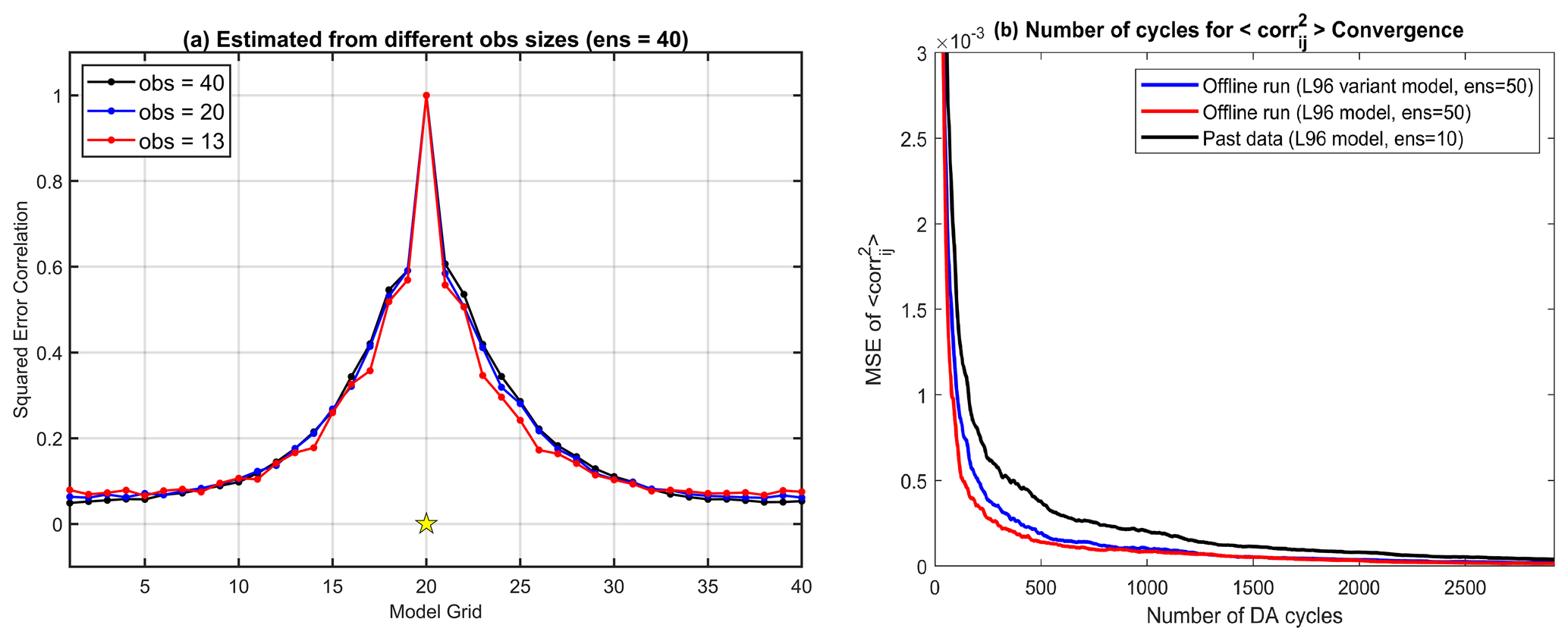
Figure 2 (a) The temporal mean squared error correlations estimated from different observation amounts. The yellow star represents the correlated observation location. (b) The MSE of Eq. (6) estimated by the past data with 10 ensembles (black) and by the ideal offline runs with the L96 model (red) and the L96 variant model (blue).

The localization functions of GDL and YK18 applied for our DA experiments are shown in Fig. 3. The optimal localization length for GDL is associated with multiple factors like ensemble size, observation distributions, and model dynamics. For example, when the ensemble size shrinks, the optimal localization length would correspondingly decrease so that a stronger suppression effect can be performed on those spurious correlations in the distant regions (Ying et al., 2018). In contrast, the YK18 localization function, once it is defined, is independent of the ensemble size changes. Unlike GDL, which provides a fixed function for every observation, YK18 offers customized localization functions for each observation based on their prior error correlations; for example, the different asymmetric features of the YK18 function (red line) in Fig. 3b and c.

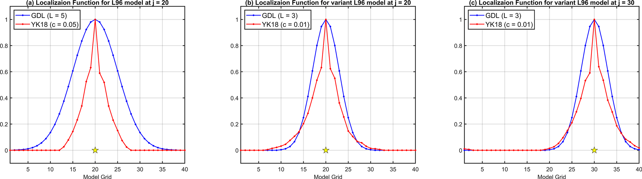
Figure 3 The localization functions of GDL (blue) and YK18 (red) for (a) the L96 model and (b, c) the variant L96 model but for the different observation sites. The yellow stars represent the corresponding observation sites. The results presented here are for the case of 10 ensembles and 40 observations.

4.2 Scenario I: classic L96 model

In this section, the classic L96 model was utilized to investigate the impacts of GDL, YK18, and Hybrid. The total experiment period is 1 year (after the first 60 cycles of spin-up) with a DA window of 6 h. The tested ensemble sizes are 8 and 10. Observations are uniformly distributed with a total number of 20 and 40. The parameters for the localization and inflation for the experiments are shown in Table 1.

Table 1 The parameters used in the L96 model experiments given in Eqs. (4) and (7). The symbol α represents the multiplicative inflation parameter.

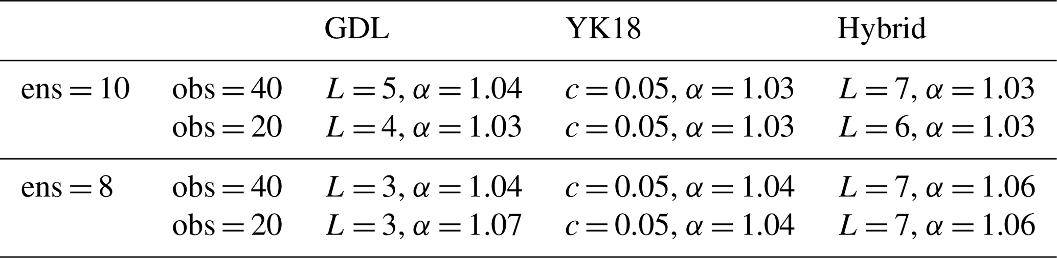
Figure 4 shows the analysis RMSE of GDL, YK18, and Hybrid. The YK18 presented the lowest RMSEs among all the methods during the DA spin-up period (Fig. 4), particularly when the ensemble size and observations were reduced (Fig. 4d). This result shows that YK18 can shorten the DA spin-up and perform an analysis comparable to GDL. The DA spin-up means the required period for the ensemble-based DA system to build a reliable background error covariance, and the analysis error reaches convergence. The phrase “spin-up” used in the following sections refers to the DA spin-up.

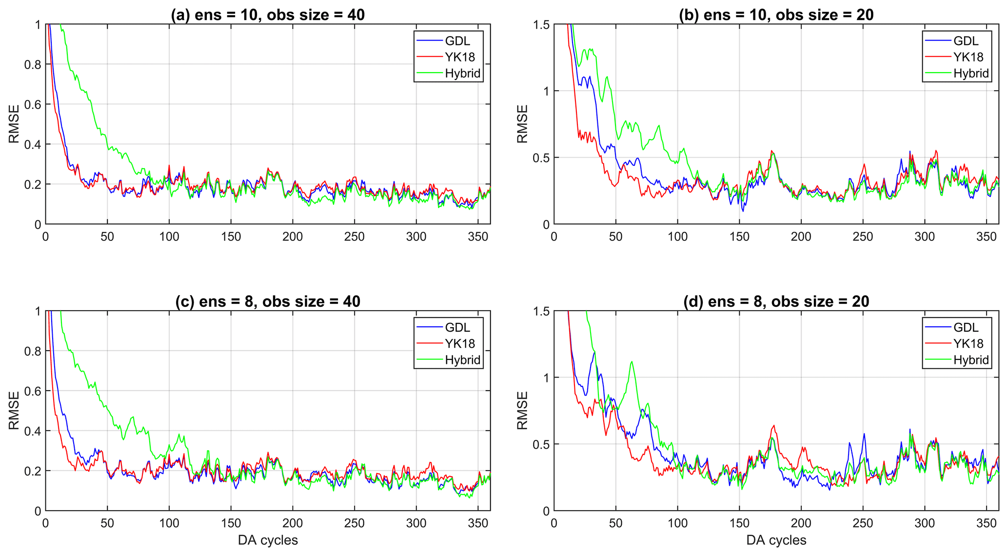
Figure 4 The time series of the analysis RMSE for GDL (blue line), YK18 (red line), and Hybrid (green line) for the cases of 10 ensembles with (a) 40 and (b) 20 observations; and cases of 8 ensembles with (c) 40 and (d) 20 observations.

The capability of YK18 in accelerating the spin-up mainly comes from its more precise interpretation of the error correlations derived from the independent (or past) ensembles. Figure 5 shows the localized background error covariance ($\mathit{\rho }{\mathbf{X}}_{\mathrm{b}}{\mathbf{X}}_{\mathrm{b}}^{\mathrm{T}}$) of GDL (blue line) and YK18 (red line) at the first (Fig. 5a) and the second (Fig. 5b) DA cycles. The true covariance (black line) was obtained by perturbing the truth state and evolving through the corresponding DA window (6 h) with a large ensemble size of 5000, which can be seen as an optimal estimation without sampling errors. At the first DA cycle, where GDL and YK18 were initialized with the same ensembles, it is apparent that the localized error covariance of YK18 is significantly closer to the true covariance, showing less spurious than GDL, especially for distant covariances (Fig. 5a). With a better estimate of the background error covariance, YK18 performed a superior analysis at the initial cycle and subsequently improved the background error estimation for the next cycle (Fig. 5b). Thus, with prior knowledge of the error correlations, YK18 can optimize the use of observations, inducing more “on-point” corrections for the analysis and reducing the required number of cycles for the DA system's spin-up. This advantage of YK18 is also present in the variant L96 model (Fig. 5c, d).

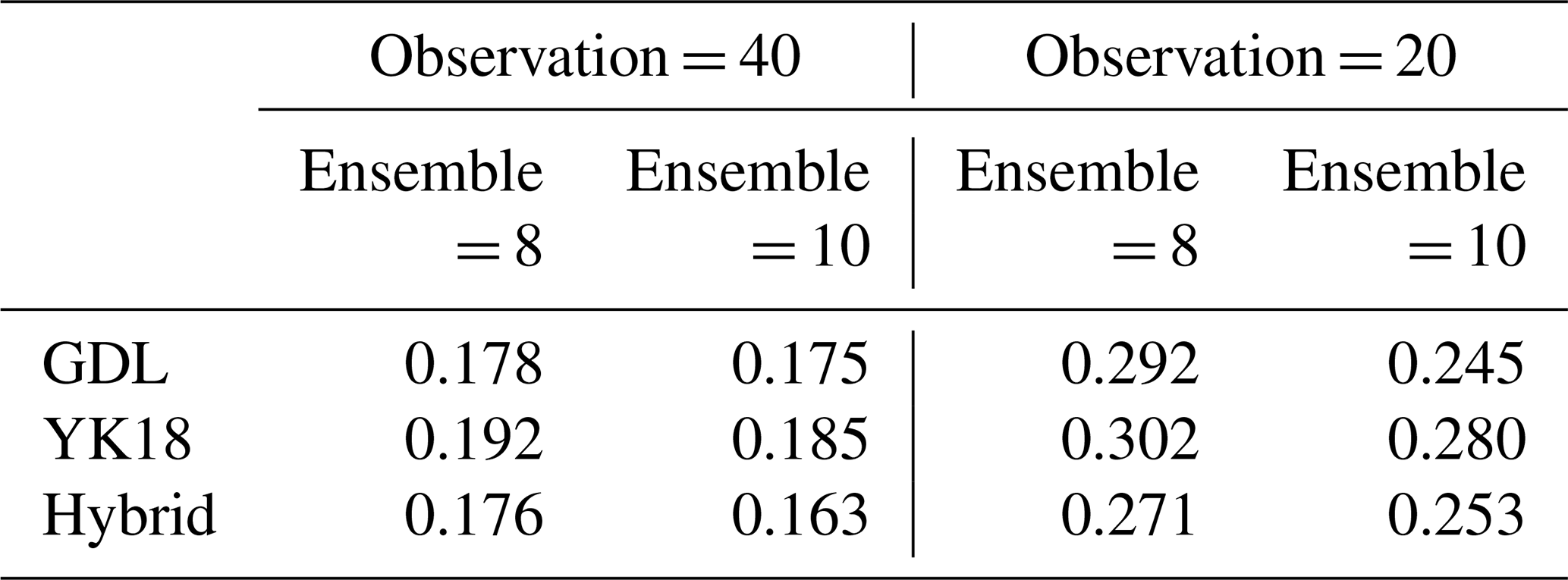
Table 2 shows the 1 year mean analysis RMSE without the spin-up period (first 100 cycles). Generally, the long-term averaged performance of the three localizations is very similar (Table 2), while Hybrid is slightly better than the other two. The best localization length for Hybrid is longer than pure GDL, which allows it to gain more observation information after the DA convergence. Note that it is unlikely for GDL to apply such a long localization length at the beginning because it needs a relatively shorter localization length to constrain the spurious error covariances during the spin-up. In our experiments, the GDL went through filter divergence at the early stage when using localization lengths larger than 7. In contrast, by averaging with the tighter function from YK18, the Hybrid was able to get through the spin-up with a longer localization length. However, on the other hand, it requires a significantly longer spin-up period than the other two methods due to its weaker constrain in the early stage.

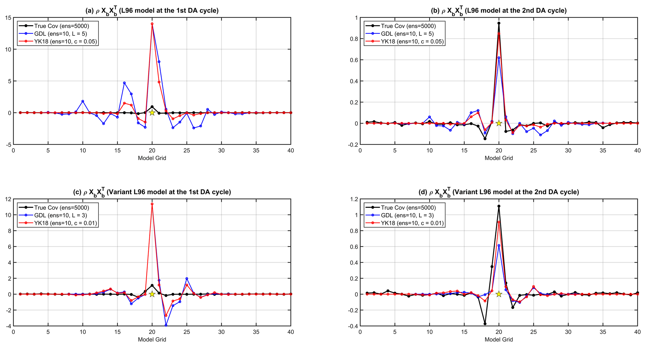
Figure 5 The true (black) and localized background error covariances ($\mathit{\rho }{\mathbf{X}}_{\mathrm{b}}{\mathbf{X}}_{\mathrm{b}}^{\mathrm{T}}$) of GDL (blue) and YK18 (red) for the L96 model at (a) the first and (b) the second DA cycles, and for the variant L96 model at (c) the first and (d) the second DA cycles. The localization functions and configurations are the same as in Fig. 3.

Table 2 The long-term mean analysis RMSE for the L96 model.

4.3 Scenario II: the variant L96 model

Considering that the L96 model is favorable for GDL due to its simple model dynamics (Table 2), the variant L96 model that offers a more complicated model dynamic was employed here. We used 10 ensembles and tested with different observation sizes of 40, 30, and 20. The 20 and 40 observations are distributed uniformly. The 30 observations are distributed densely on the land (20 observations) and coarsely in the ocean area (10 observations). Here, three localization methods were tested: GDL, YK18, and Hybrid II. Hybrid II uses YK18 for the first 80 DA cycles for accelerating the spin-up, then GDL for the rest of the cycles. Since the parameters are respectively tuned for each method, the localization length used in GDL and Hybrid II may differ. The parameters used for this section are listed in Table 3.

Table 3 The parameters used in the variant L96 model experiments given in Eqs. (4) and (7). The symbol α represents the multiplicative inflation parameter.

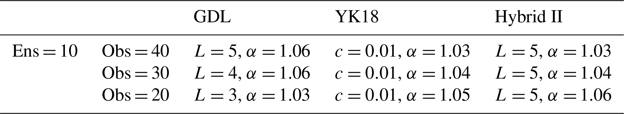
Figure 6 shows the analysis RMSE of the three methods on the variant L96 model. Note that Hybrid II is identical to YK18 for the initial 100 DA cycles, so the green overlaps with the red line in Fig. 6. As expected, GDL requires a significantly longer spin-up for the more complex model, especially when fewer observations were assimilated (Fig. 6b and c). The YK18, again, showed impressive efficiency in accelerating the spin-up, particularly with fewer observations, and generated a better analysis than GDL at the early stage (Fig. 6). Nevertheless, this advantage of YK18 became more pronounced with a more complicated model and fewer observations.

Table 4 The long-term mean analysis RMSE for the variant L96 model (10 ensembles).

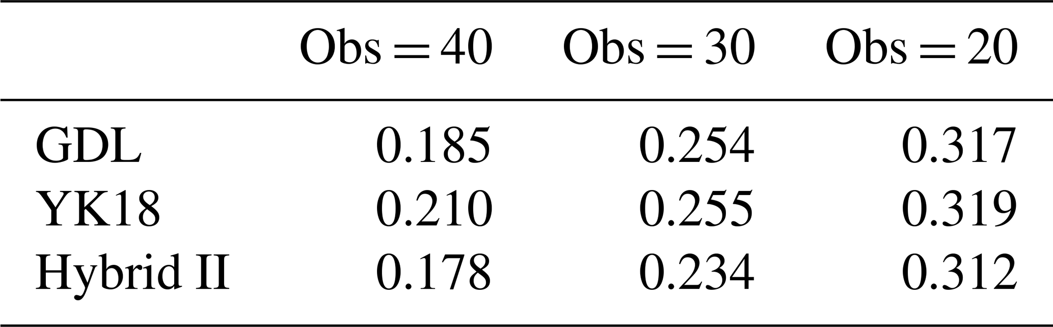
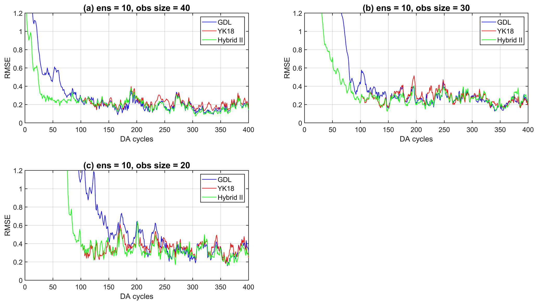
Figure 6 The analysis RMSE of the GDL (blue), YK18(red), and Hybrid II (green) with observations of (a) 40, (b) 30, and (c) 20 for the variant L96 model experiment.

Table 4 is the 1-year average of the analysis RMSE after the first 100 spin-up cycles. After the system's spin-up, the averaged analysis RMSEs of all methods are similar, while Hybrid II is slightly better than the other two methods (Table 4). We found that the mixed use of YK18 and GDL Hybrid II is superior to solely using YK18 or GDL. Hybrid II inherits the benefit of YK18 of accelerating spin-up and outperforms GDL after the system convergence, presenting the best performance among all methods. This is possibly due to the fact that Hybrid II has a longer optimal localization length than GDL, allowing it to acquire more observation information during the assimilation and provide a more accurate analysis. Moreover, Hybrid II has a significantly shorter spin-up than Hybrid I, making it a better hybrid strategy for the case that requires DA spin-ups.

Finally, it is important to highlight that YK18 is an exceptionally efficient localization method. In practice, using GDL requires multiple preceding trials to find an optimal length for the experiments of interest, which may consume considerable computational resources and time. Moreover, when the ensemble size or observation amount changes, the optimal localization length may vary accordingly, so additional tuning for the localization length might be needed for GDL. In contrast, YK18 only needs one offline run to determine the error correlations, whereas it performs an analysis comparable to GDL, even with a faster spin-up. Although an initial tuning for the parameter c in Eq. (7) is necessary at the beginning, once it is tuned, it can adapt to future ensemble or observation size changes since it is not sensitive to the variation of those factors. This feature, on the other hand, allows YK18 to avoid further trial-and-error tunings and be more efficient than GDL.

5 Summary and discussion

This study explored the feasibility of using the correlation cutoff method (YK18, Yoshida and Kalnay, 2018; Yoshida, 2019) as a spatial localization and compared the accuracy of the two types of localization, correlation-dependent (YK18) and distance-dependent (GDL), preliminarily on the L96 model with the LETKF. We also proposed and explored the potential of the two types of hybrid localization applications (Hybrid and Hybrid II). Our results showed that YK18 performs an analysis similar to GDL but with a significantly shorter spin-up, especially when fewer ensembles and observations are presented. The YK18 can accelerate the spin-up by optimizing the use of observations with its prior knowledge of the actual error correlations, effectively reducing the required number of cycles toward the analysis convergence. In our experiments with the variant L96 model, we demonstrated that these advantages of YK18 would become even more pronounced under a more complicated dynamic.

It is worth highlighting that YK18 is more efficient and economical than GDL. Traditionally, the use of GDL requires multiple trial-and-error tunings to define the optimal localization length for the experiments of interest. In contrast, YK18 only needs one offline run to obtain the prior error correlations, whereas it provides an analysis comparable to GDL even with a faster spin-up. For operational or research centers that have plentiful archives of historical ensemble datasets, it is possible to directly obtain the required prior error correlation for YK18 from the past data (i.e., historical ensemble forecasts) without executing additional offline runs.

We found that the hybrid methods, the combination uses of YK18 and GDL, generated a more accurate analysis than those solely using GDL or YK18. Hybrid II has the same advantages as YK18 in accelerating the spin-up and a larger optimal localization length than GDL. These features allow Hybrid II to spin up quicker, obtain more observation information after the system convergence, and generate a slightly better analysis than GDL and YK18. Since the imbalanced analysis would be relaxed by a larger localization length (Lorenc, 2003; Greybush et al., 2011), we expect that the hybrid methods would deliver a more balanced analysis than GDL with a multivariate model. Further investigation of this advantage will be part of our future works.

We would like to emphasize that the L96 model used in this study is highly advantageous to GDL because of its univariate and simple dynamic without teleconnection features. As a result, the two known problems in GDL, imbalanced analysis and losing long-range signals, would not appear to degrade its performance here. Despite that, this model is still an excellent test bed for preliminary DA studies because it offers a simple and ideal environment for first exploring the fundamental characteristics of new methods. With that in mind, it is encouraging that YK18 performed an analysis comparable to GDL (even with a shorter spin-up) under such an environment that is particularly advantageous to GDL. We believe YK18 has great potential to generate a relatively accurate and balanced analysis in a more sophisticated, multivariate model than GDL. More studies with a multivariate and more realistic model would be required and will be conducted as our future works.

Another future work will be extending the use of YK18 to location-varying observations. One potential solution is to use neural networks to estimate corresponding error correlations for YK18 applications (Yoshida, 2019). The experiments of Yoshida (2019) proved that neural networks could estimate the background error correlations for observation at arbitrary locations. Although high computational costs and numerous samples are inevitable for training neural networks, once the network is developed, it can provide significant advantages in estimating the error correlations for location-varying observations such as satellite data.