the Creative Commons Attribution 4.0 License.
the Creative Commons Attribution 4.0 License.
 | 08 Jul 2022
Observations of shoaling internal wave transformation over a gentle slope in the South China Sea
Steven R. Ramp
Yiing Jang Yang
Ching-Sang Chiu
D. Benjamin Reeder
Frederick L. Bahr
Four oceanographic moorings were deployed across the South China Sea continental slope near 21.85∘ N, 117.71∘ E, from 30 May to 18 July 2014 for the purpose of observing high-frequency nonlinear internal waves (NLIWs) as they shoaled across a rough, gently sloping bottom. Individual waves required just 2 h to traverse the array and could thus easily be tracked from mooring to mooring. In general, the amplitude of the incoming NLIWs tracked the fortnightly tidal envelope in the Luzon Strait; they lagged by 48.5 h and were smaller than the waves previously observed to the southwest near the Dongsha Plateau. Two types of waves, a waves and b waves, were observed, with the b waves always leading the a waves by 6–8 h. Most of the NLIWs were remotely generated, but a few of the b waves formed locally via convergence and breaking at the leading edge of the upslope-propagating internal tide. Waves incident upon the moored array with amplitude less than 50 m and energy less than 100 MJ m−1 propagated adiabatically upslope with little change of form. Larger waves formed packets via wave dispersion. For the larger waves, the kinetic energy flux decreased sharply upslope between 342 and 266 m, while the potential energy flux increased slightly, causing an increasing ratio of potential-to-kinetic energy as the waves shoaled. None of the waves met the criteria for convective breaking. The results are in rough agreement with recent theory and numerical simulations of shoaling waves.
- Article
(36207 KB) - Full-text XML
- BibTeX
- EndNote


Considerable fieldwork has now been dedicated to observing and understanding the very large-amplitude, high-frequency nonlinear internal waves (NLIWs) in the northeastern South China Sea (SCS). It has now been well established that the waves emerge from the internal tide which is generated by the flux of the barotropic tide across the two ridges in the Luzon Strait (Buijsman et al., 2010a, b; Zhang et al., 2011). Both tidal conversion and dissipation are high around the ridges (Alford et al., 2011), but adequate energy survives to escape the ridges and propagate WNW across the sea. As they do so, the internal tides steepen nonlinearly until eventually the NLIWs are formed (Farmer et al., 2009; Li and Farmer, 2011; Alford et al., 2015; Chang et al., 2021a). The longitude where this takes place depends on the details of the forcing and stratification, but based on satellite imagery, it is not until at least 120∘30′ E, roughly 50 km west of the western (Heng-Chun) ridge (Jackson, 2009). This longitude is hypothesized to be the minimum distance/time required for the internal tide to nonlinearly steepen and break, or perhaps the first point where tidal beams intersect the sea surface west of the western ridge. Once the NLIWs have formed, they propagate WNW across the deep SCS basin with remarkably little change of form (Alford et al., 2010; Ramp et al., 2010). Once the waves start to shoal on the continental slope however, roughly between 1000 to 150 m depth, the changes become quite dramatic. Wave refraction due to the shallower depth and changing stratification tends to align the wave crests with the local topography. Incident NLIWs which were initially solitary may form packets via wave breaking or dispersion (Vlasenko and Hutter, 2002; Vlasenko and Stashchuk, 2007; Lamb and Warn-Varnas, 2015). Some very large waves may split into two smaller waves (Small, 2001a, b; Ramp et al., 2004). When the wave's orbital velocity exceeds the propagation speed, usually between 300–150 m depth, the largest waves may break and form trapped cores that transport mass and nutrients onshore (Farmer et al., 2011; Lien et al., 2012, 2014; Rivera-Rosario et al., 2020; Chang et al., 2021b). Still farther onshore where the upper layer thickness exceeds the lower, the depression waves are transformed into elevation waves (Orr and Mignerey, 2003; Duda et al., 2004; Ramp et al., 2004; Liu et al., 2004). The elevation waves presumably continue propagating WNW towards shore and dissipate in shallow water, but observations to the west of this point are scarce.
Two types of NLIWs, called a waves and b waves, have been repeatedly observed, a parlance first coined by Ramp et al. (2004). Based on the Asian Seas International Acoustics Experiment (ASIAEX) results, the a waves consisted of rank-ordered packets that arrived at the same time every day and were generally larger than the b waves, which were usually solitary and arrived 1 h later each day. It has subsequently been shown via longer data sets that the timing is not universal and that b waves may sometimes be larger than a waves (Alford et al., 2010; Ramp et al., 2010). It is now recognized that the a waves are generated in the southern portion of the Luzon Strait and the b waves to the north (Du et al., 2008; Zhang et al., 2011; Ramp et al., 2019). The b waves are subject to massive dissipation over the shallow northern portion of the western (Heng-Chun) ridge (Alford et al., 2011), but the a waves are not. The distinction matters because the energy and propagation direction of the trans-basin waves incident on the continental slope determines how they behave as they shoal. These differences are explored further in this paper.
The present study was motivated by the discovery of large (h>15 m, λ order 350 m) undersea sand dunes on the sea floor along a transect southeastward from 21.93∘ N, 117.53∘ E in the northeastern South China Sea (Reeder et al., 2011). Subsequent multi-beam echo sounder surveys (MBESs) during 2013 and 2014 revealed that the dunes occupy at least the region spanning 21.8 to 21.9∘ N and 117.5 to 117.7∘ E (Fig. 1). This region is on the continental slope slightly northeast of the Dongsha Plateau. The bottom slope in the dunes region is relatively slight with respect to steeper bottom slopes progressing both offshore and onshore from the dune field. The sand dunes are of interest due to their impact on shallow-water acoustic propagation and their interaction with shoaling internal tides and NLIWs traveling WNW up the slope. The acoustic issues are addressed in other papers emerging from the program (Chiu and Reeder, 2013; Chiu et al., 2015). Oceanographic questions of interest include the following: (1) how are NLIWs transformed as they shoal over a gentle slope between 388 and 266 m over the continental slope? (2) What are the physical mechanisms responsible for this transformation? (3) How does the increased bottom roughness in the dune field affect energy dissipation in the shoaling internal tides and NLIWs, relative to other locations? Geophysical problems of interest include the following: (4) What, if any, is the role of the NLIW in sediment resuspension and dune building? (5) What determines the spatial scales of the dunes? (6) Why are the dunes located where they are, and why are they not observed elsewhere?
This paper addresses how the high-frequency nonlinear internal waves were transformed under shoaling, while the NLIW dissipation and role in the dune-building process will be addressed in separate works (Helfrich et al., 2022). The data and methods are described in Sect. 2, the NLIW arrival patterns and their relation to the source tides in Sect. 3, and the wave transformations and energy conservation in Sect. 4. A summary and conclusion section follows.
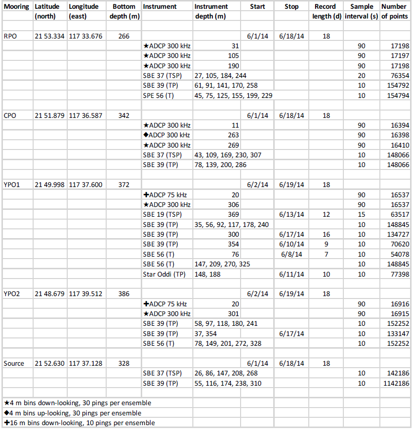
An array of four oceanographic moorings were deployed across the continental slope from 21.81∘ N, 117.86∘ E (386 m) to 21.89∘ N, 117.56∘ E (266 m) during 31 May to 18 June 2014 (Fig. 1, Appendix A; all times are given throughout in GMT). The moorings labeled YPO2, YPO1, CPO, and RPO were separated by 4.10, 3.30, and 5.69 km respectively, corresponding to wave travel times of 36.5, 30.3, and 56 min between moorings. Temperature and salinity were sampled at 60 s intervals. Instrument spacing ranged from 15 m to a maximum of 30 m in the vertical to resolve internal wave amplitudes. Currents at RPO were sampled using three downward-looking 300 kHz acoustic Doppler current profilers (ADCPs) moored at 27, 105, and 184 m depth, which provided coverage of the entire water column, except the upper 20 m. Currents at CPO were also sampled using three 300 kHz ADCPs, one downward-looking unit moored at 15 m depth, and an up/down pair at 264 m depth. Since the range of these instruments was nominally 100 m, there was an unsampled region spanning roughly 115–164 m depth at mooring CPO. Currents at YPO1 and YPO2 were sampled using one 75 kHz and one 300 kHz ADCP. The 75 kHz instruments were mounted downward-looking in the top syntactic foam sphere at 20 m depth. The 300 kHz instruments were also mounted downward-looking in cages at 300 m depth. The 300 kHz instruments burst-sampled for 20 s every 90 s, while the 75 kHz instruments sampled once per second and were averaged to 90 s intervals during post-processing. These sampling rates were adequate to observe the shoaling NLIWs with no aliasing. A fifth mooring labeled “source” on roughly the same isobath as CPO (Fig. 1) sampled temperature only from 27 to 267 m. This mooring was targeted for the same “trough” in the sand dune field as CPO to examine along-crest acoustic propagation. It additionally proved useful to identify the precise phasing and orientation of the internal wave crests in the along-slope direction.
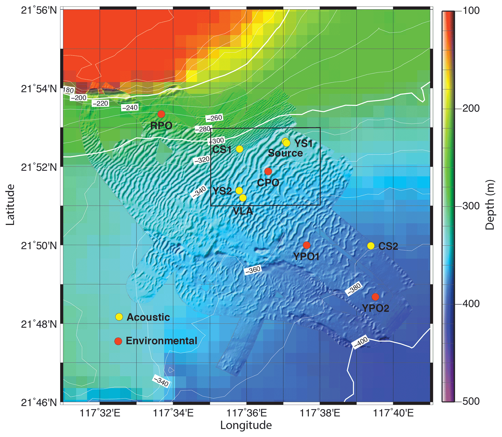
Figure 1Locator map for the Sand Dunes 2014 field experiment. This paper primarily concerns the environmental moorings indicated by the red dots, although temperature from the “source” mooring is also used. The area within the black box is expanded in Fig. 2.
3.1 The nature of the dunes
The stage is set by a zoomed-in view of the study region showing the sea floor sand dunes as depicted by the MBES data (Fig. 2). A change in the bottom slope forms a very clear line of demarcation between lower (4 m) dunes with shorter (100 m) wavelength and the larger (10–15 m) dunes with longer (260 m) wavelength. Dunes in these regions were nearly sinusoidal. Farther down the slope in water >360 m depth, the dunes were “parted”, meaning the trough widths were much greater than the crest widths. Mooring RPO was located in the first region with steeper slope, CPO was in the second region of smaller slope and large sinusoidal dunes, and moorings YPO1 and YPO2 were in a region with similar mean bottom slope but parted dunes. Repeat MBESs indicated that during 2013–2014, the dunes were stationary to within the accuracy of the surveys. For purposes of this paper, the most important fact about the bottom is the sharp, clear change of bottom slope across the dotted white line (Fig. 2) from over the shallower part to over the deeper part. These slopes are essential for comparing the observations to theory.
3.2 Wave arrival patterns
While fine-tuning the NLIW generation problem is beyond the scope of this paper, the fundamental properties of the wave arrival patterns can be understood via comparisons with the generating tide in the Luzon Strait. Having no remote observations during spring 2014, the wave arrival patterns at the sand dunes moored array were compared with the barotropic tidal forcing in the Luzon Strait as obtained from the TPXO7.0 global tidal model (Egbert and Erofeeva, 2002). The model output has been shown to be in good agreement with the limited observations available in the Luzon Strait (Ramp et al., 2010) and is thus a good indication of the tidal amplitude and phase at generation.
To begin, all the NLIWs arriving at the moored array were identified using large-scale plots of temperature, salinity, and velocity. The arrivals were then summarized for the entire time series by labeling the displacement of the 20∘C isotherm from its mean position at mooring RPO (Fig. 3a). The wave arrivals, as indicated by sharp downward displacements of the isotherm, fall into two groups or “clusters” of waves, each within a fortnightly envelope. The waves were labeled using previous conventions, using lowercase a and b for the first cluster and uppercase A and B for the second for uniqueness. This nomenclature will be used to refer to individual waves subsequently.
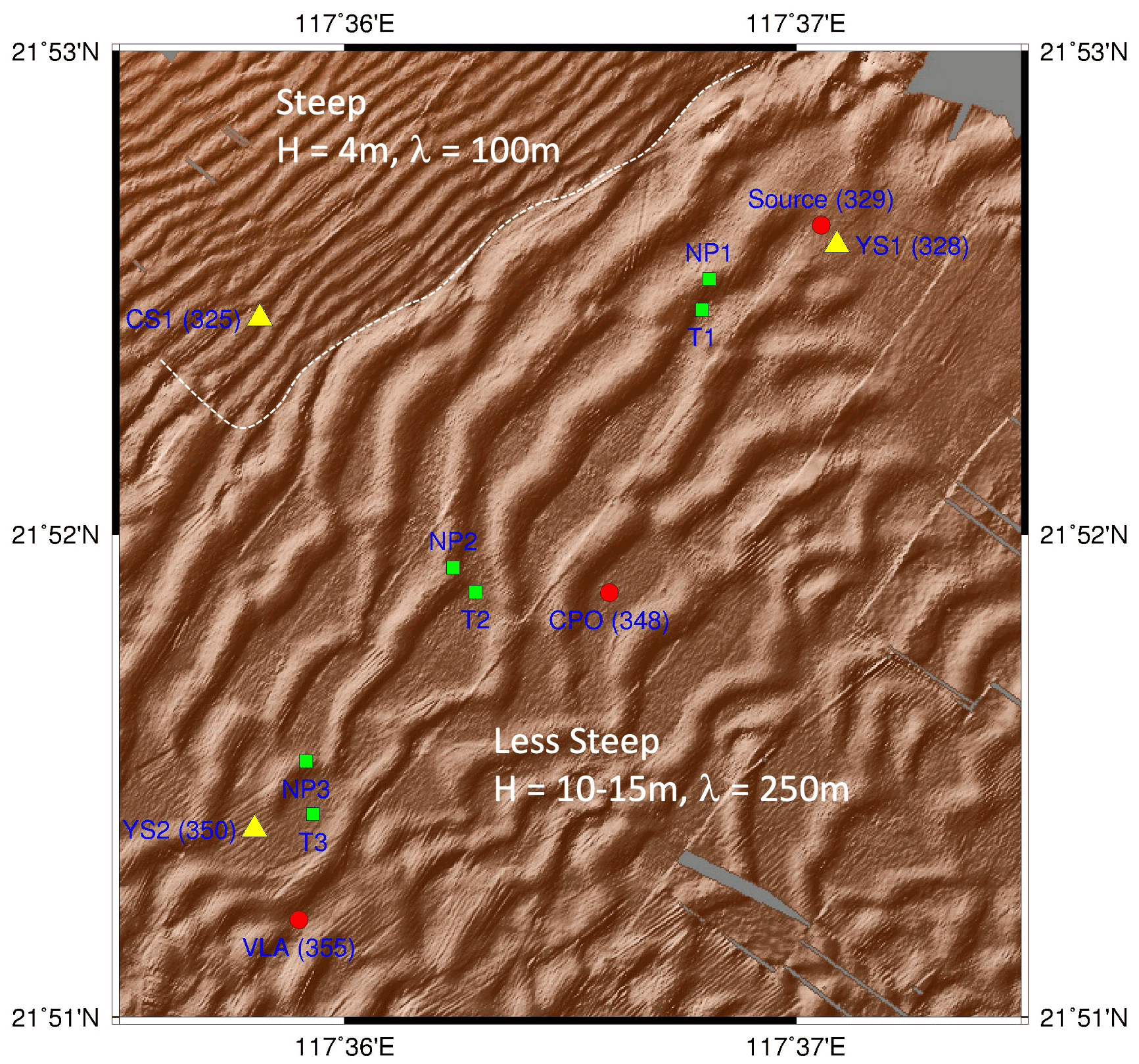
Figure 2The sea floor in the study region as observed by a multi-beam echo sounder (MBES) survey during June 2014. The region is delineated by the black box in Fig. 1. The dotted white line indicates a sharp change in bottom slope, steeper towards the northwest.
There is no dynamical difference implied by the upper- vs. lowercase names. A total of 21 NLIWs with amplitude greater than 20 m were observed, 13 a waves and 8 b waves. When b waves were present, the waves arrived in b and a pairs, with the b wave always leading the a wave by on average 6.6 h. The a waves began arriving earlier in the fortnightly cycle, for instance, 7 to 11 June. The b waves began arriving later and grew larger later in the fortnightly cycle. With the exception of 3 and 15 June, the a waves were larger than the b waves.
The RPO wave amplitude time series was then plotted over the Luzon Strait tides (Fig. 3b) with the wave amplitudes lagged by the propagation time from the source to the mooring. The lag time (48.5 h) was estimated by making a small adjustment to the propagation time nearby (50.3 h), which was calculated using a full year's data (Ramp et al., 2010). Several obvious results emerge from this comparison. First, the NLIW amplitudes at RPO track the fortnightly tidal amplitudes in the Luzon Strait. The largest waves were generated at spring tide in the strait, and no waves at all were generated during neap. This result is consistent with longer (11-month) time series obtained over the continental slope to the southwest (Chang et al., 2021a). Second, the generating tide was mixed, diurnal dominant, with a strong diurnal variation, but only the major beats resulted in NLIWs in the far field. The minor beats and the neap tides were apparently too weak to spawn NLIWs downstream. As a result, just one wave of each type was generated per day, despite the generating tide being semidiurnal. The major and minor beats switched positions during the neap tide, and the wave arrivals at the sand dunes array switched positions accordingly. Third, the lagged a waves aligned precisely with the major ebb (eastward) tide in the Luzon Strait, in agreement with previous work. This suggests generation by the lee wave mechanism (Buijsman et al., 2010a). Finally, the b waves were sometimes aligned well with the major flood tide preceding each a wave, but we now believe this to be coincidence: the directional histograms (not shown) show the a waves on average traveling along a path about 24∘ more northward (294∘) than the b waves (270∘), consistent with the primary source for the a waves being located farther to the south along the Luzon ridge system. The b waves lead because their generation site was closer to our observation point on the Chinese continental slope.
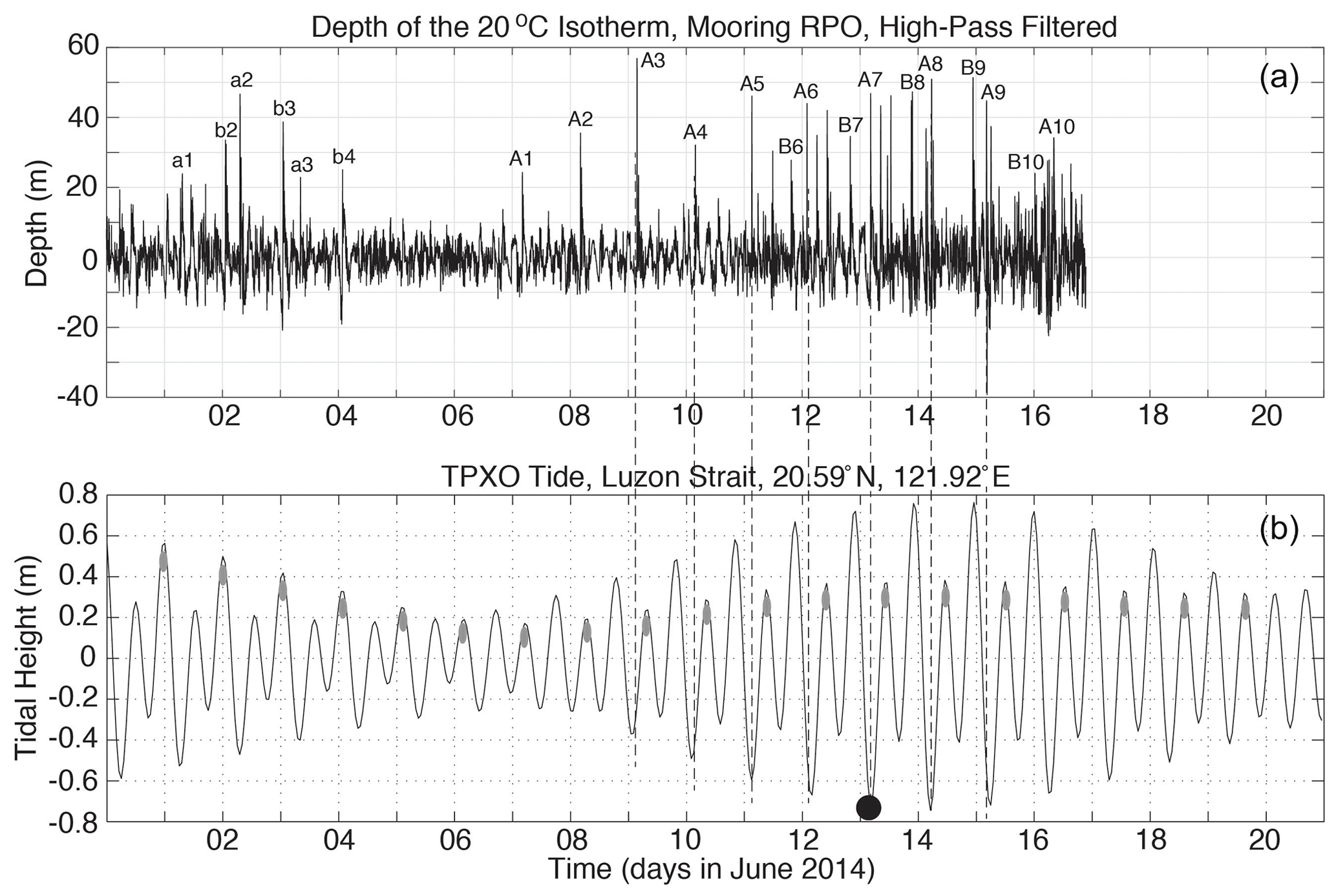
Figure 3(a) Time series showing the depth of the 20∘C isotherm observed by mooring RPO located at the 266 m isobath (Fig. 1). The time series was high-pass-filtered to separate thermal displacements due to NLIWs from the internal tides and mean (mesoscale and seasonal) flows. The sharp depressions of the isotherm indicate passing NLIWs. The type-a and type-b waves are labeled using lowercase for the first fortnight and upper case for the second. (b) Barotropic tidal amplitude in the central Luzon Strait from the TPXO global tidal model (Egbert and Erofeeva, 2002), at a point located between Batan and Itbayat Island in the Luzon Strait. The gray ellipses indicate how the major and minor tidal beats switched positions during the neap tide. The black circle indicates the time of the full moon on 13 June. The waves (a) have been lagged by the propagation time from the strait (48.5 h) to better align with the barotropic tidal envelope in the generating region. The vertical dashed lines show how the lagged a waves aligned with the ebb tide in the straits.
One example of the daily moored temperature time series at mooring RPO is shown to further illustrate these results (Fig. 4). During 9 to 13 June, the A waves arrived at about the same time each day, while from 14–18 June, they arrived about an hour later each day. This result, that the A wave arrival times were constant early in the fortnightly tidal cycle but were delayed an hour per day as the waves increased in amplitude later in the cycle, was consistent with the model results of Chen et al. (2013). Wave A7 on 15 June was anomalously late by about 2 h relative to waves A6 and A8. This is attributed to the passing of tropical storm Hagabus on 14–15 June with accompanying strong wind-forced currents and upper ocean mixing. The B wave arrivals began at about 20:00 on 13 June and were subsequently delayed about an hour per day, similar to the corresponding A waves (Fig. 4). The difference in the arrival times between the B waves and the A waves was 06:30, 08:25, 06:15, and 05:50 on 14–17 June respectively. Wave B7 was not delayed by the storm, which provides further evidence for different propagation paths for the B waves vs. the A waves. On 16–18 June two A waves of near equal amplitude arrived about 2 h apart. These “double A waves” appeared over the slope only near spring tide in the Luzon Straits, and the second one was designated by a prime. The origin of these waves is unclear. We speculate that the new A' waves originated from a different (third) source in the Luzon Straits that is only active under maximum barotropic forcing. More observations in the source region are needed to understand the wave generation issues, including this double a-wave phenomenon.
3.3 Wave transformation over the slope
Many significant wave transformations were observed between the 386 (YPO2) and the 266 m (RPO) isobaths over the upper continental slope. Three sections of the record are shown to illustrate different phenomena. The first sequence from 2 to 6 June (Fig. 5) evolved out of moderate and decreasing forcing in the Luzon Strait (Fig. 3). The observations captured the local steepening and breaking of the tidal front to form b waves as it shoaled. The internal tides at YPO2 were diurnal and nearly sinusoidal with an amplitude of about 4∘C (blue line). The a waves were already evident at YPO2 but not the b waves. Then, beginning at YPO1 and continuing to CPO, the leading edge of the tidal front became very steep, with a temperature change of 1∘C min−1 for 5 min at CPO (black ellipses in Fig. 5). This front subsequently broke and formed b-wave packets b2 and b3 observed at mooring RPO. This example thus demonstrates a local b-wave formation process via steepening of the leading edge of the tidal front. This steepening temperature front was due to velocity convergence at the head of the westward-propagating internal tide. The formation of a similar bore-like feature at shallower depths (200–120 m) was noted in the ASIAEX data (Duda et al., 2004), but they did not make the connection to b-wave formation. Waves a1 and a2 lost amplitude and formed packets as they shoaled between YPO2 and RPO. This process will be compared with some recent theoretical ideas in the “Discussion” section. Wave a3 was small at YPO2 but gained amplitude as the tide progressed up the slope. This is because the barotropic forcing in the Luzon Strait was weaker on 5 June than on 2–4 June (Fig. 3). All the waves subsequently disappeared on 7–8 June during neap tide in the Luzon Strait.
The second sequence during 10–14 June shows well-developed A-wave packets which originated from moderate but increasing remote forcing (Fig. 6). Only A waves were observed until 13 June when the B waves started to arrive. Wave B6 was weakly perceptible at YPO2 and increased in amplitude across the slope. The temperature fluctuations induced by the A waves increased across the slope and reached a maximum of 7∘C on 11 June at A3. The temperature gradients in the wave fronts were again very steep, 1∘C min−1. The number of waves per packet increased towards shallower water, most clearly in waves A2, A3, and A4. Two extraneous solitary waves appeared trailing wave A5 on 13 June at CPO and RPO but were not part of the A5 packet structure. Two similar waves appeared the next day trailing wave A6 (Fig. 7), and their origin is unclear.
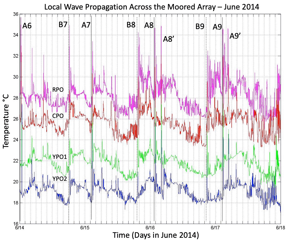
The final sequence from 14 to 18 June was obtained during a period of maximal forcing near spring tide at the source, and a very complicated field of NLIW emerged (Fig. 7). The B waves were large and were evident at all the moorings. Wave B8 and B9 were solitary at YPO2 but had many waves per packet by the time they reached RPO. The arrival timing was the same as the locally formed b waves (Fig. 5), suggesting similar dynamics but faster/shorter development time/distance when the forcing at the source was stronger. The A waves continued to grow at YPO2 during 14–18 June. Interestingly, the temperature fluctuations due to the largest waves did not increase monotonically as they traveled up the slope from YPO2 to RPO. This is more clearly seen in a bar graph showing the maximum amplitude of the isotherm of maximum displacement (Fig. 8). Smaller waves (9–12 June) gained amplitude as they shoaled. All waves larger than about 50 m offshore (13–18 June) lost amplitude as they shoaled, most clearly between CPO and RPO, where the biggest change in bottom depth and slope occurred. This result is consistent with the numerical results of Lamb and Warn-Varnas (2015), who also found that smaller-amplitude waves continued to gain amplitude into shallower water, but the larger waves did not. This fundamental result, that NLIWs first gain amplitude and then lose it as they shoal, is consistent with EKdV (extended Korteweg–de Vries) theory(Small, 2001a, b; Vlasenko et al., 2005). Note that all the wave amplitudes (Fig. 8) were smaller than those observed previously over the continental slope 44, 87, and 145 km to the southwest (Ramp et al., 2004; Lien et al., 2014; Chang et al., 2021a; Ramp et al., 2022). This is because, as seen in hundreds of satellite images (typified by Fig. 9), the NLIWs have maximum amplitude in the region just north of the Dongsha Plateau near 20∘ N, decreasing both northward and southward from there. Along-slope observations have also shown a reduction in the upslope energy flux off-axis towards the northeast (Chang et al., 2006). The sand dunes site is near the northeastern extremity of the wave crests, as viewed in the imagery: a bit farther to the northeast, the waves vanished. A practical ramification of this is that the undersea sand dunes were located in a region where the forcing due to encroaching NLIWs was not maximal. Other factors such as the bottom slope and sediment supply must also play an important role in determining the dune formation location.
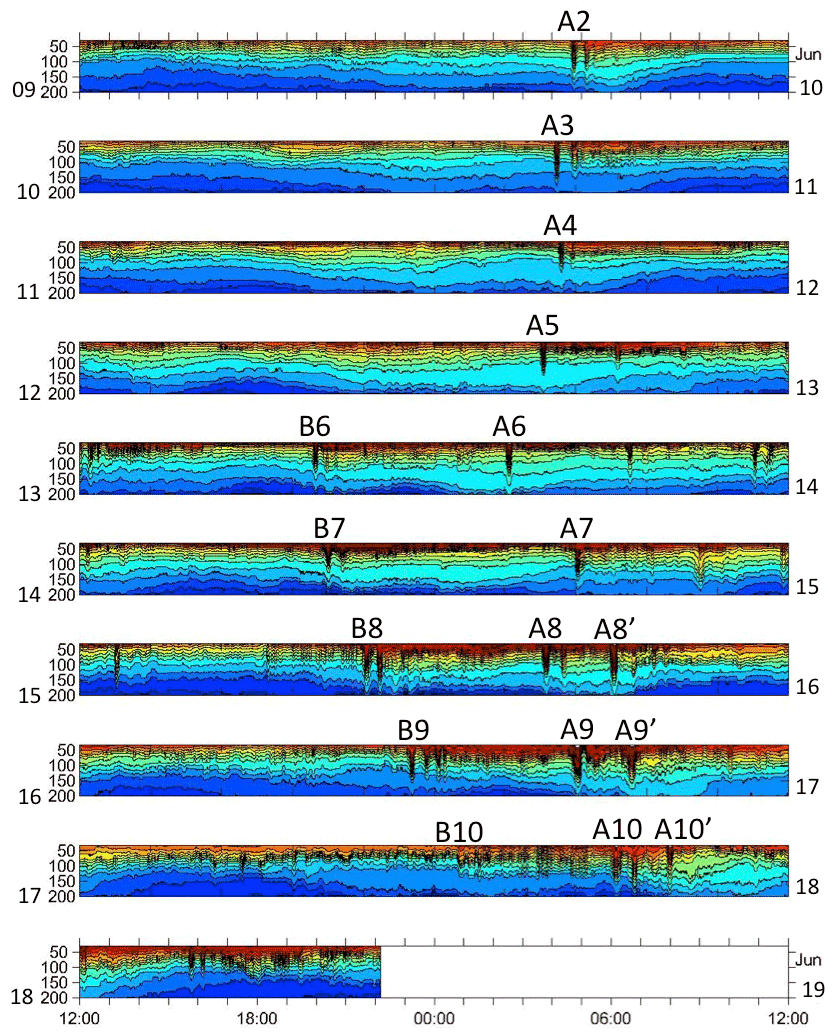
Figure 4Temperature contour plots for mooring RPO from 9 to 19 June 2014. Each panel from top to bottom is 1 d centered on midnight, to capture both the A- and B-wave arrivals. The A waves were prominent throughout this fortnightly cycle. The B-wave arrivals began on 13 June, 5 d after the A-waves. The double A waves (A8'–A10') arrived only during 16–18 June. This and similar plots were used to label the waves in Fig. 3.
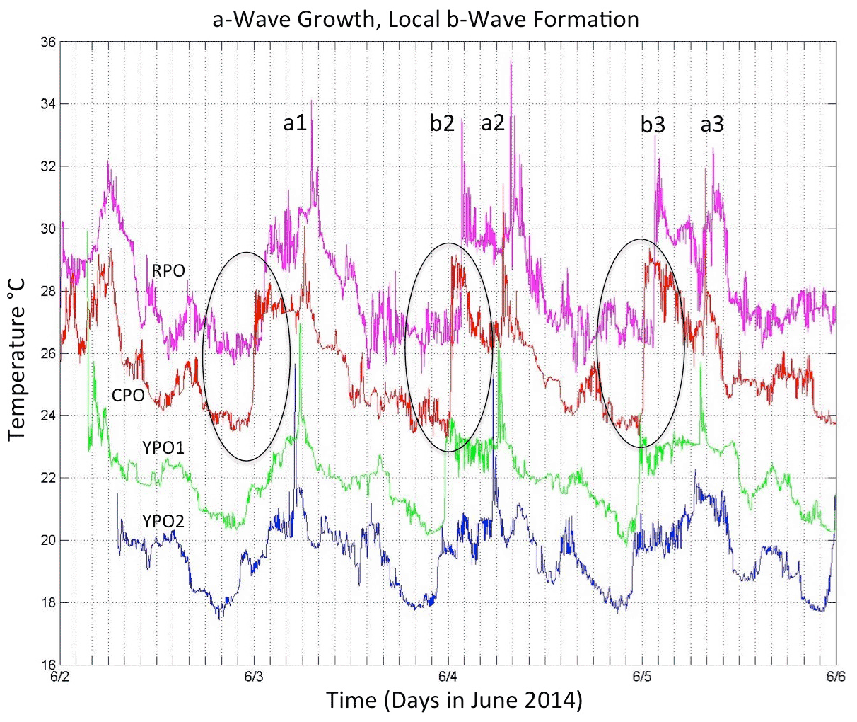
Figure 5Temperature vs. time during 2–6 June at all four moorings across the continental slope. The observations are from 75, 79, 97, and 99 m from moorings RPO, CPO, YPO1, and YPO2 respectively. Each time series has been offset vertically by 2∘C for clarity. The black ellipses highlight the region of strong temperature fronts at CPO that subsequently broke and formed b waves at RPO.
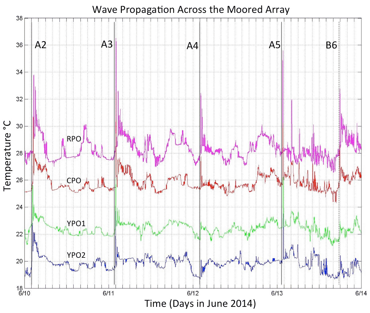
Figure 6As in Fig. 5, except during 10–14 June 2014. In this plot, the time series have additionally been shifted relative to YPO2 by the propagation time between moorings so that individual waves line up. The lag times used are 36.5 min for YPO1, 66.8 min for CPO, and 122.8 min for RPO.
The double a-wave phenomenon mentioned earlier (Fig. 4) was again evident in Fig. 7. These waves differed from the smaller waves trailing A5 and A6 in that they were already well developed by the time they arrived at YPO2. As in Fig. 6, many waves which were solitary at YPO2 formed packets as they crossed the array. Waves B9, A9, and A9' can be clearly seen in the satellite ocean color imagery (Fig. 9). The timing of the imagery at 03:10 was conveniently just as wave A9 was impacting mooring YPO2. The B-wave packets and solitary nature of A9 and A9' are easily seen in the image.
Two examples of velocity and temperature across the slope are shown to illustrate the difference between weakly and strongly forced waves. Mooring YPO1 is not shown since it was very similar to mooring YPO2 (Fig. 10). The weaker case begins at YPO2 on 3–4 June (Fig. 10, column 1) which shows a clear a wave near 0530 but no b wave. Wave a2 was observed towards the rear of the northwestward-propagating internal tide (blue near the surface). The a wave was traveling NW near the surface and in the opposite direction in the lower water column, with a nodal point near 100 m. While not obvious in temperature, the velocity plots show a weak second wave about 20 min behind the lead wave forming a two-wave packet. By mooring CPO (column 2), located 7.3 km away, the leading edge of the internal tide had steepened to form a sharp front in both velocity and temperature near midnight on 3 June. There was strong convergence in the upper 50 m with eastward flow (red shades) ahead of the front and westward flow (blue shades) behind it. A solitary b wave appeared on this convergent front, which was absent at YPO2. Wave a2 at CPO looked similar to YPO2, perhaps slightly stronger. By mooring RPO, 5.7 km and 80 m farther up the slope (column 3), the b wave increased in amplitude and formed a two-wave packet, and the leading a wave spawned a four-wave packet. These waves were particularly clear in the v component since the waves refracted towards the north as they propagated up the slope (Fig. 1). The nodal point remained near 100 m for all the leading waves. Note that the background internal tide (most easily seen in the deep water) was diurnal at moorings YPO2 and CPO but became more semidiurnal at RPO. This indicates the presence of a locally generated tide at RPO where the bottom slope was steeper than at the other moorings farther offshore. In fact, the bottom slope at YPO2-CPO (Figs. 1, 2 right of the dotted white line) was critical to the diurnal tide, while the slope at RPO (left of the dotted white line) was critical to the semidiurnal tide. The interaction of the tidal currents with the bottom is maximal where the slope of the tidal beams parallels the bottom, and this likely contributes to the different nature of the sand dunes offshore vs. onshore of the dotted white line (Fig. 2). At all moorings, there was only one westward surface internal tide per day. The b waves all emerged at the leading edge of this westward tide, while the a waves emerged towards the rear, and this clear velocity signature represents another way to distinguish the two types of waves. The two wave arrivals were separated by 06:20 on this day. The strongest bottom velocities were downslope (southeast) and were greater in the NLIW than in the internal tide.
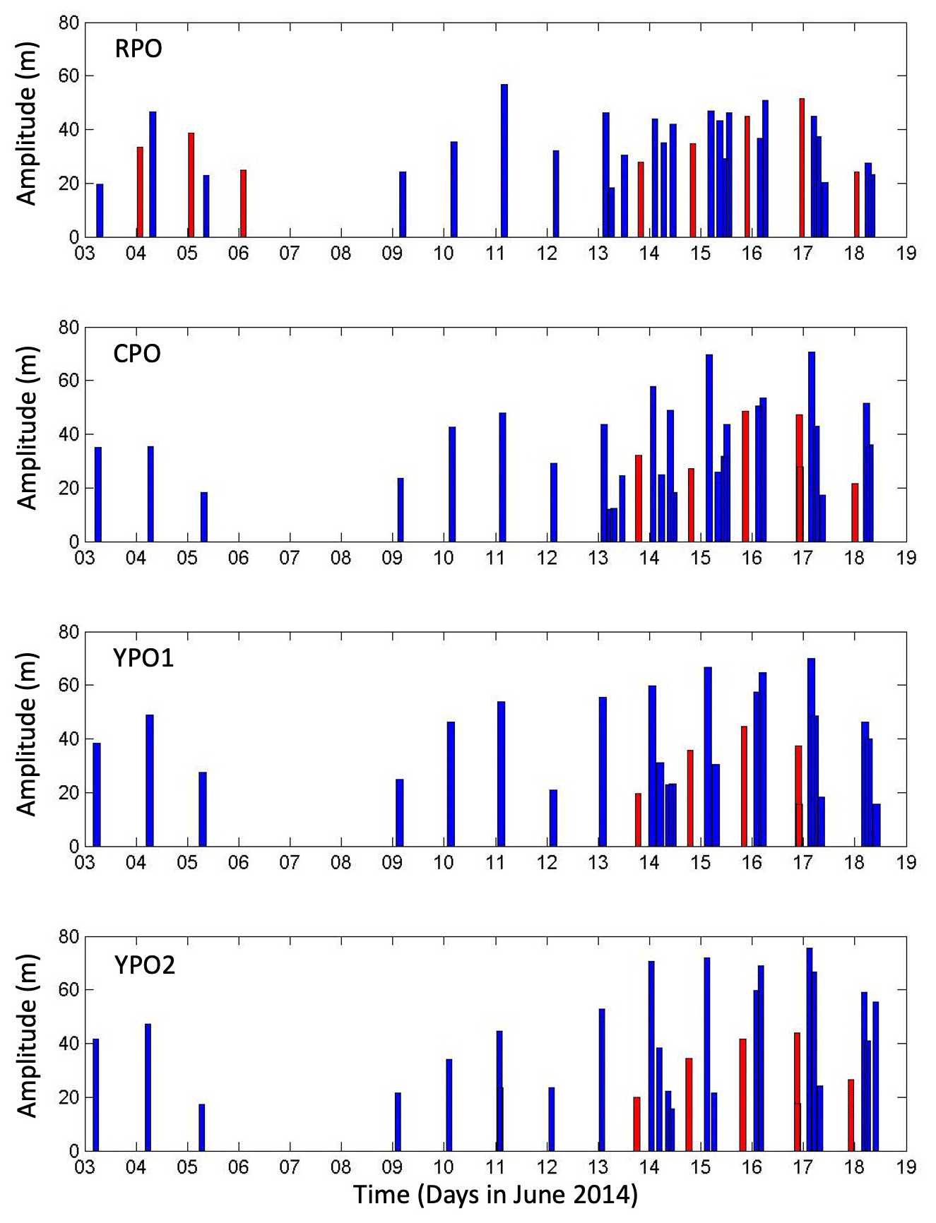
Figure 8Bar graph of wave amplitudes across the slope. The amplitudes were calculated as deviations of the 20∘C isotherm from its mean position. The a waves are indicated by blue bars and the b waves by the red.
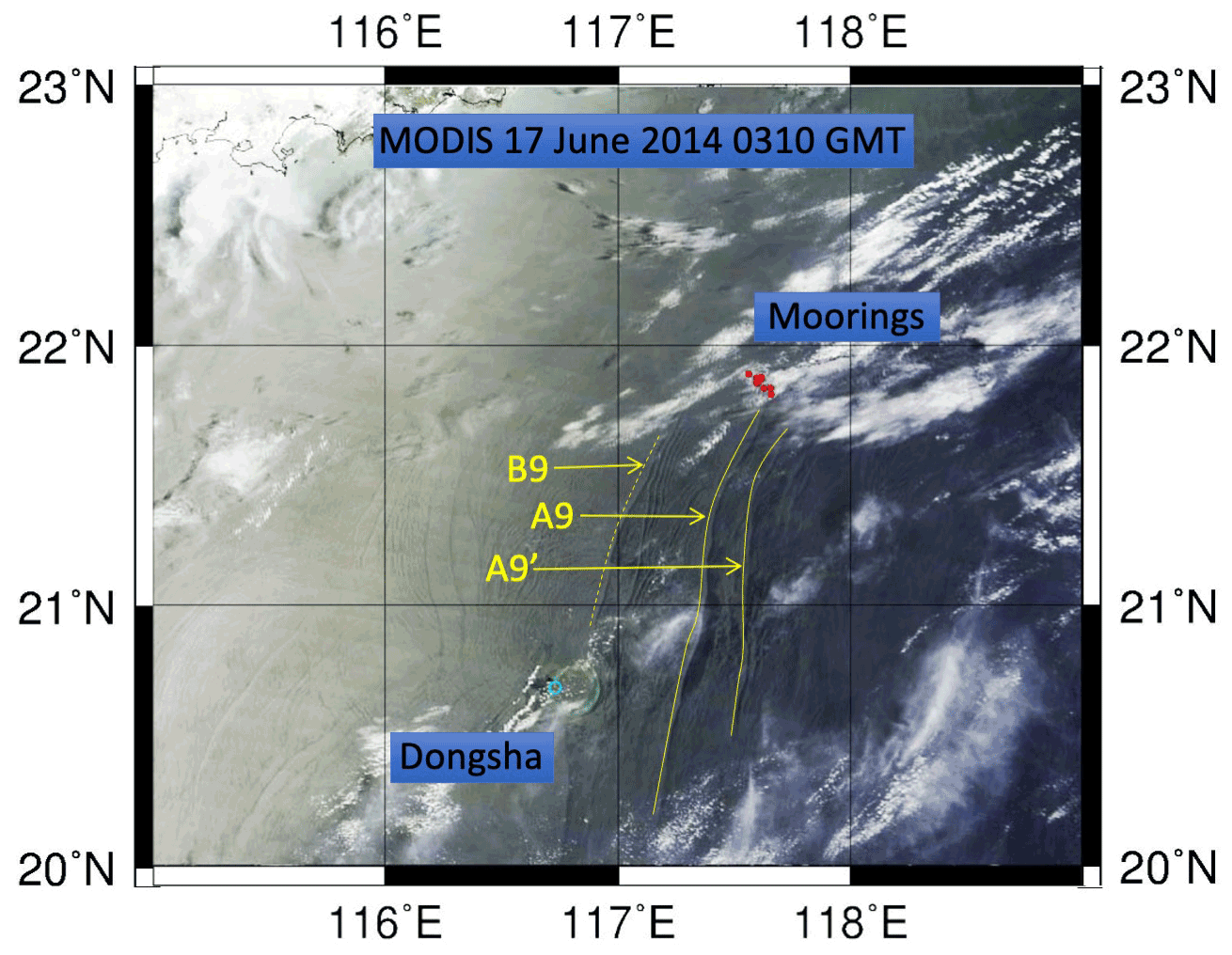
Figure 9A sea surface ocean color image obtained at 03:10 on 17 June 2014 from the Moderate Resolution Imaging Spectroradiometer (MODIS). The sand dunes moorings are indicated by the red dots. The surface signatures of NLIWs B9, A9, and A9' are indicated by the yellow arrows. Wave A9 was impinging upon mooring YPO2 at this moment, as seen in Fig. 7 (base image data courtesy of NASA, plotted using HDFLook and GMT software).
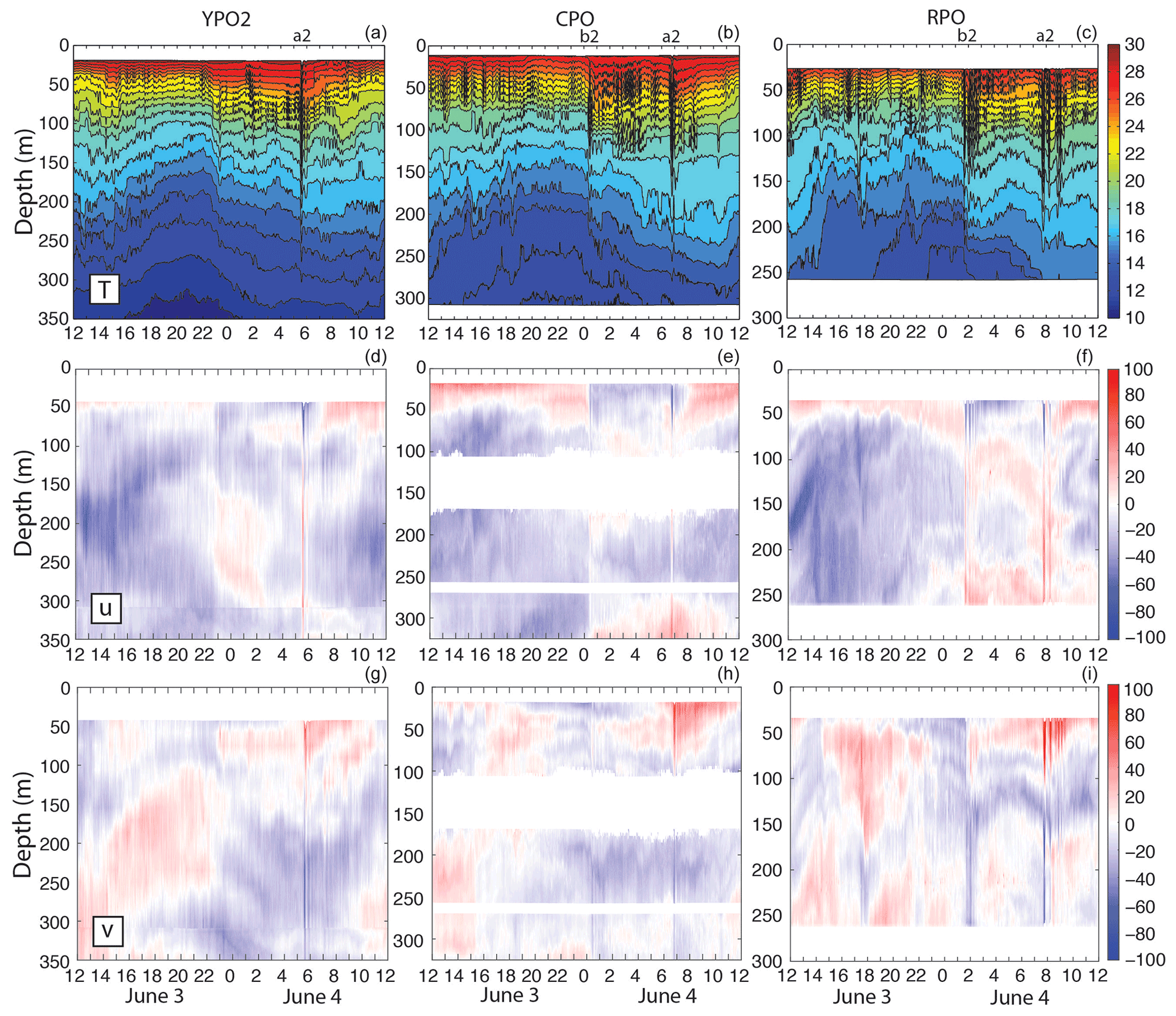
Figure 10Temperature (a–c), u component of velocity (d–f) and v component of velocity (g–i) from 3–4 June 2014 from moorings YPO2 (a, d, g), CPO (b, e, h), and RPO (c, f, i). The wave propagation time between moorings was 67 min from YPO2 to CPO and 56 min from CPO to RPO. Positive (u, v) represents (east, north) respectively. White space at mooring CPO indicates regions not sampled by the three ADCPs. These data were obtained during a period of moderate and declining tidal forcing; see Figs. 3 and 5 for context.
The strong example (Fig. 11) shows that unlike the previous example, both the B-wave packet and the A-wave packet had already formed by mooring YPO2 on 16–17 June (remember there is no dynamical significance to upper- vs. lowercase a and b: the lettering is chosen to remain consistent with the nomenclature established in the earlier figures and refers to the first and second cluster). The waves were traveling in the same direction as the 3–4 June waves but had a deeper nodal point located near 120–130 m. The A wave in this case was a double A wave mentioned earlier. These resembled individual waves rather than a packet in the usual sense. The two waves A9 and A9' were about the same amplitude: on this day the first wave (A9) was slightly larger, but the opposite was true the day before (not shown). The A9' wave was slightly wider than the A9 wave. This may be due to constructive interference with the tail of wave A9, which was just 2 h ahead of it. Wave B9 formed a two-wave packet at CPO (column 2) and a three-wave packet at RPO (column 3). Wave A9 formed a two-wave packet between moorings CPO and RPO. As before, the u component shows the B wave was coming off the leading edge of the westward surface tide (eastward bottom tide). The A9 wave grew out of the middle of the tide, and the A9' wave emerged from the trailing edge of the same westward internal tide. The surface westward velocities exceeded 97, 162, and 153 cm s−1 at YPO2, CPO, and RPO respectively. The eastward bottom velocities exceeded 20, 85, and 80 cm s−1 respectively. The smaller lower layer velocities below the nodal point were consistent with a thicker lower layer and with theory (Lamb and Warn-Varnas, 2015). The strongest bottom velocities outside the waves were about half the wave velocities. Clearly the strongest bottom velocities observed over the upper continental slope were generated by the passing NLIWs, although these high velocities were very brief compared to the internal tide. Referring once again to Fig. 8, the B wave (just before midnight on 16 June) started at YPO2 with just over 40 m amplitude and grew shoreward across the shelf. In contrast, the much larger A waves just after midnight on 17 June started out with 70–75 m amplitude at YPO2 and lost amplitude across the shelf. This is consistent with the earlier discussion surrounding Fig. 10.
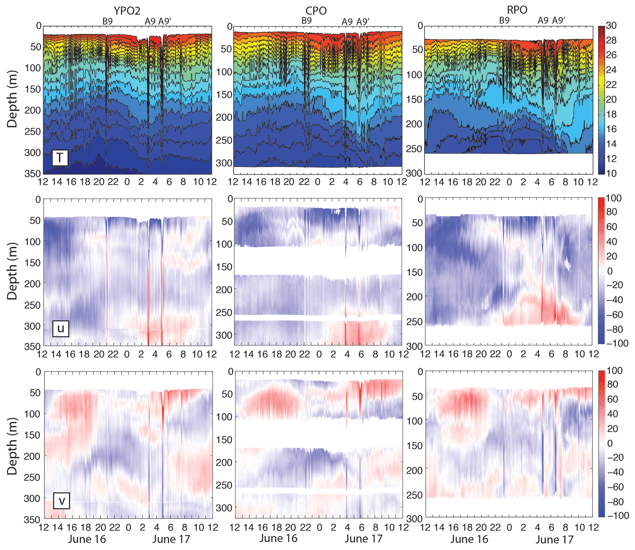
Figure 11As in Fig. 10 except for 16–17 June 2014. These data were obtained during a period of strong tidal forcing; see Figs. 3 and 7 for context.
Many ordinary internal waves can be seen in Fig. 11 in between the nonlinear waves. These waves were likely generated by tropical cyclone Hagabus, which passed over the array on 14–15 June with winds exceeding 25 m s−1.
On 16 June a packet of convex mode-2 waves appeared from 15:00–21:00, centered near 60 m and extending from 50 to 100 m depth (Fig. 11, bottom row). These waves strengthened upslope from YPO2 to RPO and trailed the double-A waves from the day before (not shown). There looked to be about six waves in the mode-2 packet at mooring RPO. All three of the double-A waves on 16, 17, and 18 June had this feature associated with them. The observation is consistent with Yang et al. (2009, 2010), who observed mode-2 waves trailing mode-1 waves in the ASIAEX region nearby and attributed this to the adjustment of shoaling mode-1 waves. These observed wave transformations are now discussed further below in light of the theory for shoaling solitary waves.
4.1 Theoretical framework
In this section, the observed NLIW characteristics are compared with laboratory and numerical studies to determine what kind of changes might be expected as the waves shoal over the sand dunes region. The possibilities include adiabatic shoaling, dispersion, breaking, and conversion to waves of elevation. The latter may be easily ruled out for this study since this only happens when the nonlinear coefficient α from the Korteweg–de Vries (KdV) equation changes sign, which typically takes place between 100–120 m depth over the Chinese continental shelf (Hsu and Liu, 2000; Orr and Mignerey, 2003; Liu et al., 2004). Even accounting for some temporal variability due to the local internal tides, this “critical point” where the upper- and lower-layer depths were equal was always well inshore of the sand dunes region.
The wave progression WNW from deeper to shallower water may be conveniently framed in terms of the two regions demarcated by the dotted white line in Fig. 2. Moorings YPO1, YPO2, and CPO were all located in the region where the mean bottom slope was . Mooring RPO was in the region where the bottom slope was . The bottom slope is considered gentle when it is less than (Grimshaw et al., 2004; Vlasenko et al., 2005; Lamb and Warn-Varnas, 2015; Rivera-Rosario et al., 2020). Dynamically speaking, the mean bottom slopes in the sand dunes region then ranged from weak to practically flat. Under these conditions, the response of shoaling NLIWs depends primarily on three factors: the bottom depth, wave amplitude, and thermocline depth (Small, 2001a, b; Vlasenko and Hutter, 2002; Lamb, 2002; Vlasenko and Stashchuk, 2007; Grimshaw et al., 2014; Lamb and Warn-Varnas, 2015; Rivera-Rosario et al., 2020). Waves break when wave orbital velocity umax> the propagation speed c (Lien et al., 2014; Rivera-Rosario et al., 2020; Chang et al., 2021b) and
where am is the maximum possible wave amplitude, Hb is the bottom depth, and Hm is the upper layer thickness, here approximated by the thermocline depth (Helfrich and Melville, 1986; Helfrich, 1992; Vlasenko and Hutter, 2002). This expression can be used to evaluate the isobath where a wave of given amplitude will break or, alternatively, to determine the wave amplitude necessary for wave breaking at a given isobath. For the upslope-propagating waves observed here, these criteria were examined for moorings CPO in region 1 and RPO in region 2. The depth of the 23∘C isotherm was used to estimate the thermocline depth at both moorings. The undisturbed isotherm depth, determined by time-averaging the low-pass-filtered data, was similar at both moorings, 60 m at CPO and 57 m at RPO. Substituting these values in Eq. (1) shows that a wave amplitude of 112 m would be required at CPO for wave breaking to occur. Moving on to RPO, the required amplitude for wave breaking there would be about 84 m. In comparison with the observed wave amplitudes at CPO and RPO (Fig. 8), all the observed wave amplitudes were lower than the above criteria, and no wave breaking events are expected in this array. Some combination of adiabatic shoaling and packet formation via wave dispersion is more likely instead.
Using this guidance, the temperature and velocity structure at site RPO is studied in greater detail for three examples: a statistically common a wave (Fig. 12), a very large a wave (Fig. 13), and a b wave (Fig. 14). For wave A3 on 11 June (Fig. 12), which typifies A waves between 3–13 June, the wave was symmetric in both velocity and temperature, with no sign of back-side steepening. The wave amplitude was 57 m, and the maximum orbital velocity was 1.04 m s−1 and was located near the surface. This was much less than the local propagation speed of 1.60 m s−1. The opposing lower-layer velocity was on the order of 0.75 m s−1, commensurate with the thicker lower layer. Such bottom velocities were commonly observed and are easily enough to produce both bedload and suspended sediment transport among the dunes (Reeder et al., 2011). The w profile was nearly symmetric at ±0.25 m s−1, downward ahead of the wave and upward behind it, with the maxima located near mid-depth. One or possibly two trailing waves were observed: the first was centered near 04:48 and had vertical velocities of ±0.8 m s−1, while the second was near 05:00 with vertical velocities of just a few centimeters per second. A fourth wave-like feature was observed in the temperature plot near 05:20, but it cannot be discerned in the velocity structure. To summarize, wave A3 consisted of a primary wave and two to three trailing waves about 30 min behind. The wave was symmetric in velocity and temperature, with no sign of breaking or trapped core formation.
The largest wave observed was wave A9 on 17 June. This wave showed several characteristics of breaking or near-breaking waves (Fig. 13). The back side of the wave was steeper than the leading side, and the jagged temperature contours in the wave core were indicative of breaking and/or mixing. A “pedestal” was starting to form behind the wave as described by Lamb and Warn-Varnas (2015). Several more smaller depression waves were emerging from the pedestal. The velocity contours were likewise asymmetric and showed a subsurface maximum near 60–70 m, which was about 0.20 m s−1 greater than the surface. This is typical of waves with trapped cores (Lien et al., 2012, 2014; Lamb and Warn-Varnas, 2015). The maximum near-surface velocity was 1.55 m s−1, which was close to the local propagation speed (1.60 m s−1). It is possible that the surface velocities above 20 m depth were slightly larger but were not observed. At site CPO, this same wave had a maximum velocity of 1.80 m s−1, also very close to the local propagation speed. The vertical velocities were actually smaller than wave A3, at −12 and +20 cm s−1, with at least two and possibly more of the trailing depression waves visible as down/up pairs. To summarize, this wave appears to be about to break or just starting to break; however, this wave was the exception rather than the rule: only one such wave was observed. It is possible that the trailing double-A waves A8' and A9' might also meet these criteria; however their form was distorted by interference from the trailing packet of the leading A8 and A9 waves 2 h earlier, making their characteristics difficult to discern. The South China Sea NLIW amplitudes in June are near their maximum values observed in July and August (Chang et al., 2021a). It is thus unlikely that breaking waves are ever prevalent in the sand dunes region. This situation contrasts with a similar depth range farther southwest, where larger waves were already actively breaking at the 300 m isobath (Chang et al., 2021b).
It is worth noting that the subsurface velocity maximum in the wave may be caused by phenomena other than wave breaking. Tropical cyclone Hagabus passed over the array on 14–15 June and forced strong near-surface currents which opposed the wave velocities. This was especially obvious on 15 June (not shown), when westward currents at 80 m depth in wave A7 exceeded the surface currents by over 0.80 m s−1 at RPO and by over 1.00 m s−1 at CPO. This likely explains why wave A7 arrived 2 h late with respect to waves A6 and A8 (Fig. 4). The storm also left behind a surface mixed layer 40 m deep, which lingered to the end of the record.
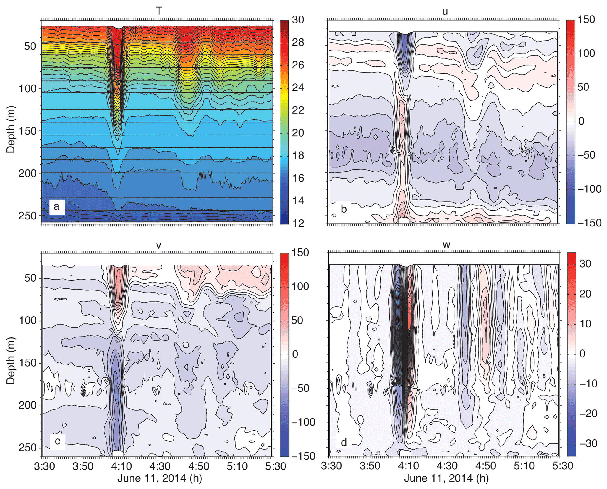
Figure 12(a) Temperature, (b) u component of velocity (positive east), (c) v component of velocity (positive north), and (d) vertical velocity (positive up) for wave A3 on 11 June 2014. This rank-ordered packet with a symmetrical leading wave typifies most of the type-a waves observed during the experiment.
This means all the largest waves forced near spring tide propagated into a region with an unusually deep surface mixed layer. The effect of this is to severely limit wave breaking (Lamb, 2002). In fact, the scenario described above in the “Results” section rather closely resembles the model results of Lamb (2002) when a surface mixed layer was added (their Fig. 10). The shoaling solitary wave in the model produced a second trailing solitary wave, followed by the dispersive tail of mode-1 depression waves, followed by a packet of mode-2 waves. The observations reported here closely resembled this pattern, not only on 16–18 June, but also on 3–5 June trailing waves a1 and a2.
We conclude that most of the packets that formed as the waves traveled up the slope from YPO2 to RPO were formed by dispersion rather than wave breaking. Rotational effects seem locally unimportant, given that the packets formed in just 2 h, while the local inertial period was 32 h. Rotation may have played a role farther offshore, establishing the initial perturbations (inertial gravity waves) that then grow and become a trailing packet as the waves shoal (Grimshaw et al., 2014). This effect could not be investigated without observations in deep water. Trailing undular bores of the sort modeled by Grimshaw et al. (2014) by including rotation were not observed but are likely not observable since in the real ocean, the waves arrive periodically, and the trailing undular bores would be destroyed by each subsequent arriving NLIW before they have a chance to develop. It is most likely then an imbalance between nonlinearity and dispersion that causes the new trailing waves to form (Vlasenko and Hutter, 2002; Lamb and Warn-Varnas, 2015). The large lead internal solitary wave (ISW) in the sand dunes array never split into two but rather slowly decreased in amplitude as energy was transferred to the dispersive tail. Phenomena such as wave splitting and breaking likely took place inshore of the sand dunes array in the vicinity of the 150 m isobath, as was observed previously at the ASIAEX site nearby.

Figure 13As in Fig. 12 but for wave A9 on 17 June 2014. The steepening back side and subsurface velocity maximum suggest breaking or imminent breaking.
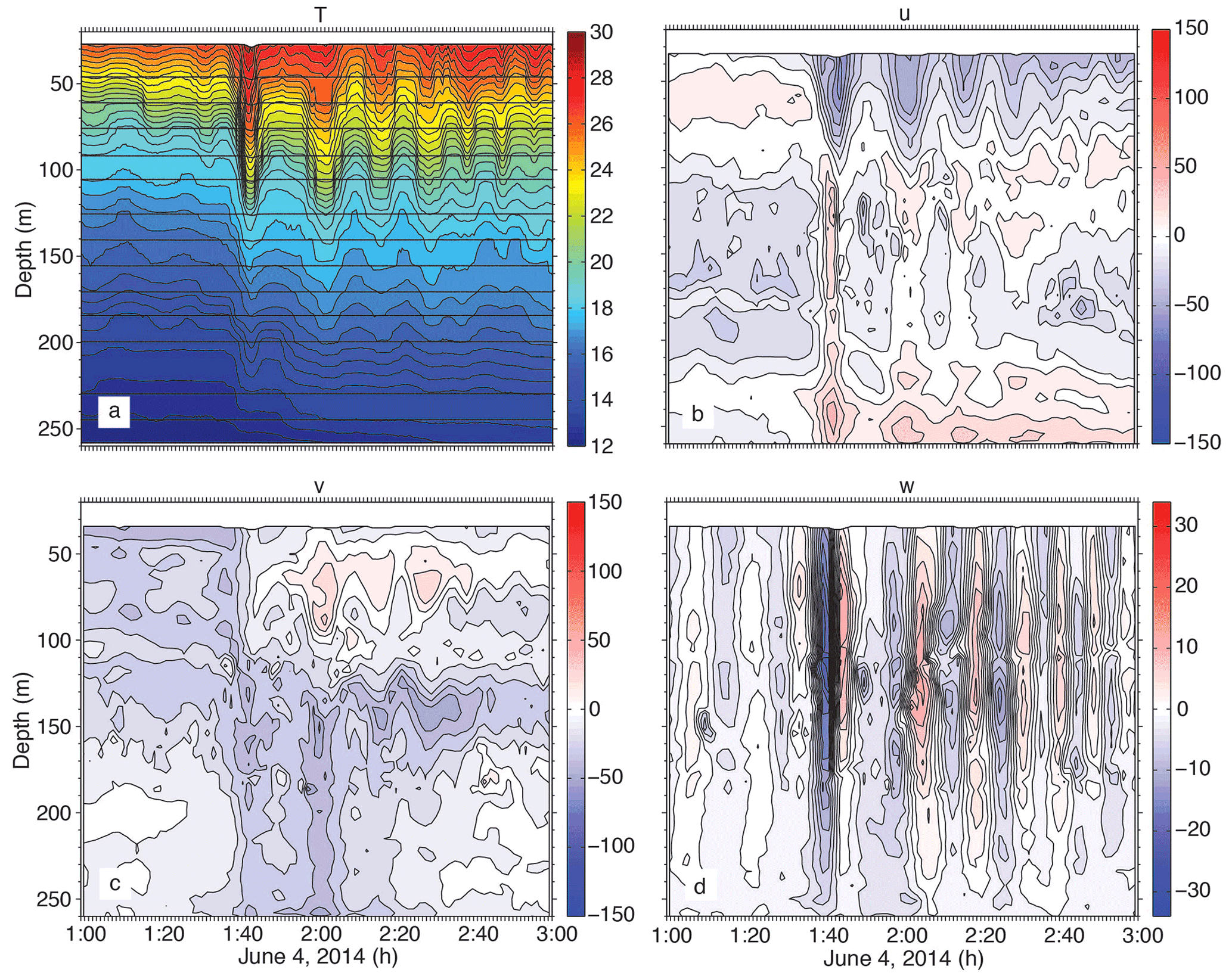
Figure 14As in Fig. 12 except for wave b2 on 4 June 2014. This example typifies waves formed locally by breaking of the tidal front between moorings YPO and RPO.
The situation for the locally formed b waves (b2–b4) was completely different. These waves were nonexistent at YPO2 but formed well-defined, evenly spaced packets by the time they reached RPO (Fig. 14). For wave b2 on 4 June, six waves can be clearly seen in T and w, with most of the horizontal velocity in u; that is these waves were traveling westward. The amplitude of the lead wave was about 40 m, the near-surface velocity 60 cm s−1 westward, and near-bottom velocity 40 cm s−1 eastward. The waves were formed all at once by the collision and breaking of the westward internal tide with the off-slope-propagating eastward tide. This is a different mechanism than that described for shoaling ISWs in the literature.
4.2 Energy and energy flux
The data set provides an opportunity to observe how the horizontal kinetic (HKE) and available potential (APE) energy in the high-frequency nonlinear internal waves changes as the waves propagate up a gentle slope. In turn, the energy pathways provide some insight into the dynamics underlying the wave transformation process. The theoretical expectation for linear and small-amplitude nonlinear internal waves is that the energy will be equipartitioned for freely propagating long waves away from boundaries. This is not the case however for finite-amplitude, nonlinear, nonhydrostatic internal solitary waves, whose kinetic energy (KE) typically exceeds the PE by a factor of 1.3. This result was found theoretically via exact solutions to the fully nonlinear equations of motion (Turkington et al., 1991) and has also been noted observationally (Klymak et al., 2006; Moum et al., 2007). Thus, the KE is expected to slightly exceed the PE for the waves arriving at mooring YPO2. For shoaling NLIW however, the flux of PE theoretically exceeds the flux of KE, which causes the PE to exceed the KE in shallower water (Lamb, 2002; Lamb and Nguyen, 2009). This is because the flux of PE remains nearly constant, while the KE flux decreases as the upper- and lower-layer thicknesses become more equal. Shoaling waves observed in the Massachusetts Bay displayed this property (Scotti et al., 2006). Thus, a shift from greater KE to greater PE might be expected as the waves shoal from YPO2 to RPO, although it depends on the details of the wave amplitude, stratification, and bottom slope, etc.
To compute the energies and energy fluxes from moorings, time series of density and velocity which are uniform in space and time are required. Moorings RPO and CPO had good coverage of temperature and salinity in the vertical (Appendix A); however moorings YPO1 and YPO2 sampled temperature only. Two methods to compute the density at YPO1 and YPO2 were explored. The first used a constant salinity (34.42, the vertical average from a nearby CTD cast) paired with the observed temperature at each sensor to compute density. This method assumes that most of the density variability comes from the temperature fluctuations rather than salinity. The second method used the salinity profiles from all the CTD casts taken during the cruise to compute a mean curve, which was then used as a lookup table to determine the salinity to use with each observed temperature. The CTD casts were all within 12 km of each other and were thus treated as a time series. The profiles fell into two groups, namely before tropical storm Hagabus passed by on 14 June, with little to no surface mixed layer, and after the storm, when the mixed layer was about 40–50 m deep. Thus, two mean curves were actually used, one from before the storm and one after. The benchmark for these methods was to compare the density calculated using the curves with the actual density calculated using the observed salinity on moorings RPO and CPO. The APE computed using the mean curve was found to agree much better with the observations than the APE computed using a constant value for the salinity. Both techniques were slight underestimates of the true APE but the method much less so than the constant method. For this reason, the mean curves were used to compute the density time series and thus APE for moorings YPO1 and YPO2.
The observed time series also had velocity gaps of varying severity in the water column due to the range limitations of the ADCPs. Mooring CPO had a mid-depth gap spanning roughly 110–170 m and a second smaller gap from 255–265 m (see Figs. 10 and 11). These gaps were filled using the least-squares-fit normal-mode techniques described in Nash et al. (2005). Theoretically as many as seven modes (number of instruments in the vertical – 1) were possible, but the most stable results were achieved with just three modes. No attempt was made to fill in the upper 20 m of the water column where both velocity and temperature were unsampled by the moorings.
Once clean time series were available to operate on, the energies and energy fluxes were computed from the data via established techniques (Nash et al., 2005, 2006; Lee et al., 2006). The baroclinic velocity and pressure fluctuations induced by the waves were first computed as
and
where
is the density anomaly with respect to the time-mean density profile. In Eqs. (2) and (3), the last term satisfies the baroclinicity requirement that the primed quantities integrate to zero over the entire water column (Kunze, et al., 2002). Overbars indicate temporal means. The HKE and APE can then be computed as
where ρ0 is the mean density, g is the acceleration of gravity, and N2 is the buoyancy frequency.
The energy flux due to highly nonlinear internal waves is given by
where the first term on the right is the pressure work, and the second and third terms represent the advection of horizontal kinetic and available potential energy density (Nash et al., 2012). For the small-amplitude, linear, hydrostatic case, the flux equation is often approximated as the first term only:
but since it is not obvious that this approximation is valid for the strongly nonlinear shoaling waves observed in the sand dunes region, all three terms of the flux equation were computed.
The resulting changes in the wave energy distribution across the slope depended on the wave amplitude (Fig. 15). For waves up to and including A3 on 11 June, the APE exceeded HKE offshore and continued to increase up the slope. This is interpreted to mean the waves were still growing and had not yet reached maximum amplitude. Smaller waves can penetrate farther upslope adiabatically than larger waves. Wave A4 was anomalously small for which no obvious explanation has been found. Perhaps the wave was obliterated by the leading edge of tropical storm Hagabus. Starting with wave A5 on 13 June, as the remote barotropic tidal forcing continued to increase, the HKE exceeded APE at YPO2 by a factor averaging 1.7 and increased to its maximum value at mooring YPO1. This ratio is even larger than the theoretical expectation of 1.3 (Turkington et al., 1991; Lamb and Nguyen, 2009) and indicates highly nonlinear waves with large amplitudes. Between CPO and RPO, there was a dramatic change when the APE increased and the HKE sharply decreased, resulting in greater APE than HKE at mooring RPO (Fig. 15a). The energy ratio at RPO (Fig. 15f) was commonly 3 to 4 but suddenly decreased sharply with the arrival of wave A6 on 14 June and remained near 1 for the remainder of the time series. This is attributed to the increased surface mixed layer depth as the tropical storm went by which wiped out the upper ocean stratification and reduced the APE. The total energies (Fig. 15e) integrated both vertically and over a wavelength followed an envelope consistent with the remote tidal forcing and maxed out at around 250 MJ m−1. This was less than half the energy (550 MJ m−1) previously reported over the Dongsha Plateau (Lien et al., 2014), where the maximum observed wave amplitudes exceeded 150 m vs. 80 m here. The total energy appears approximately conserved across the slope for many of the waves as indicated by color bars of approximately equal length (Fig. 15e). The losses in HKE were compensated for by the increases in APE, in reasonable agreement with theory and numerical simulations (Lamb and Nguyen, 2009; Lamb and Warn-Varnas, 2015). For the larger waves however, such as a1, A6, A8', A9, and A9', the total energy decreased upslope (Fig. 15e). The HKE was lost much faster than the APE was gained. This is attributed to strong dissipation over the rough bottom in the dune field (Helfrich et al., 2022).
In the simplest sense the energy flux is just the energy times the group velocity (or phase velocity for nondispersive waves). Since the phase velocity varied from 1.87 m s−1 between YPO2 and YPO1 to 1.69 m s−1 from CPO to RPO, the flux to energy ratio is expected to vary little across the slope, and the flux patterns should resemble that of the total energies. This is indeed the case as seen by comparing the envelope of the curves for the total flux (Fig. 16b) and the total energy (Fig. 15e). The vertically integrated flux tends to decrease upslope, primarily due to the decreasing water depth. Of greater interest is the change in the various terms of Eq. (7). The pressure work (PW) is indeed the largest term but not by much: the PW comprised 57 %, 56 %, 43 %, and 52 % of the total flux at YPO2, YPO1, CPO, and RPO respectively. The large percentage still remaining was accounted for by the advection of HKE and APE and shows that the waves were indeed strongly nonlinear. The increase in APE with respect to HKE at mooring RPO versus CPO can be accounted for by the change in the fluxes at those moorings (Fig. 16a). From CPO to RPO, the kinetic energy flux dropped by 50 % (blue line to green line), while the potential energy flux went up slightly (red line to purple line).
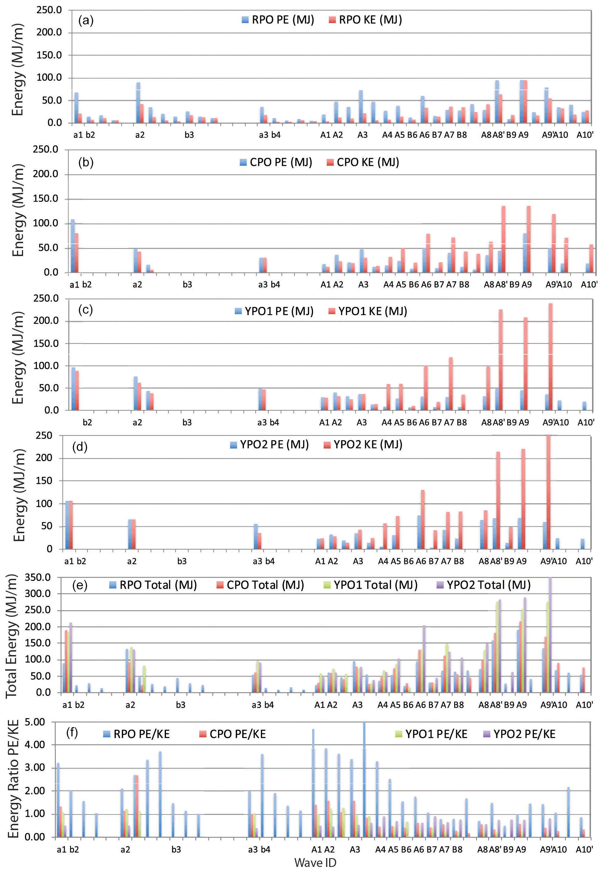
Figure 15Energy transformations across the slope. The total HKE and APE, computed by integrating the wave energy both vertically and horizontally at moorings RPO, CPO, YPO1, and YPO2, are shown in (a)–(d) respectively. The total pseudo-energy (HKE + APE) at all four moorings is shown for each wave in (e) and the APEHKE ratio in (f).
An 18 d time series of high-resolution velocity and temperature data were obtained at four closely spaced moorings spanning 386–266 m depth on the continental slope 160 km northeast of Dongsha Island in the South China Sea. The experiment was motivated by the need to understand ocean variability and how it interacts with large (15 m) sand dunes on the sea floor. The dominant signal observed consisted of sets of large-amplitude, nonlinear internal waves (NLIWs) impinging on the continental slope from the southeast. These were in fact the very same waves that impact the Dongsha Island region and have been reported by many previous authors. The sand dunes waves however were about 50 % smaller and less energetic than the Dongsha waves, since the location was near the northern extremity of the wave crests rather than near the main axis of the waves. The mean bottom slope along the sand dunes mooring line was also gentler than farther southwest. While the internal tides are no doubt important to the dune-building process, this paper focuses entirely on the NLIW properties, most especially how the waves were transformed as they shoaled up a very gradual bottom slope. New information gleaned includes the packet formation process, further insights on the difference between a waves and b waves, and the energy transformation processes which took place during wave shoaling.
During the fortnight observed, the a waves began arriving several days ahead of the b waves and traveled in a more northerly direction. Once they started arriving, the b wave always lead the a wave by 6–8 h. In any given pair, the a wave was generally larger, but b waves generated near spring tide may be larger than a waves generated near neap. The a waves generally arrived at the site as two to three wave packets, but the b waves may also form packets as they shoal. The wave generation location and their positioning relative to each other and the internal tide determine the wave classification. The b waves were located near the head of the upslope internal tide, while the a waves developed more towards the back. The wave arrival patterns rigorously tracked the tidal structure in the Luzon Strait, even to the point of shifting by 6 h when the alternating strong-beat followed by a weak-beat pattern reversed in the strait during neap tide. The arrival patterns were consistent with earlier work showing that the a waves were generated in the southern portion of the Luzon Strait and the b waves in the north.
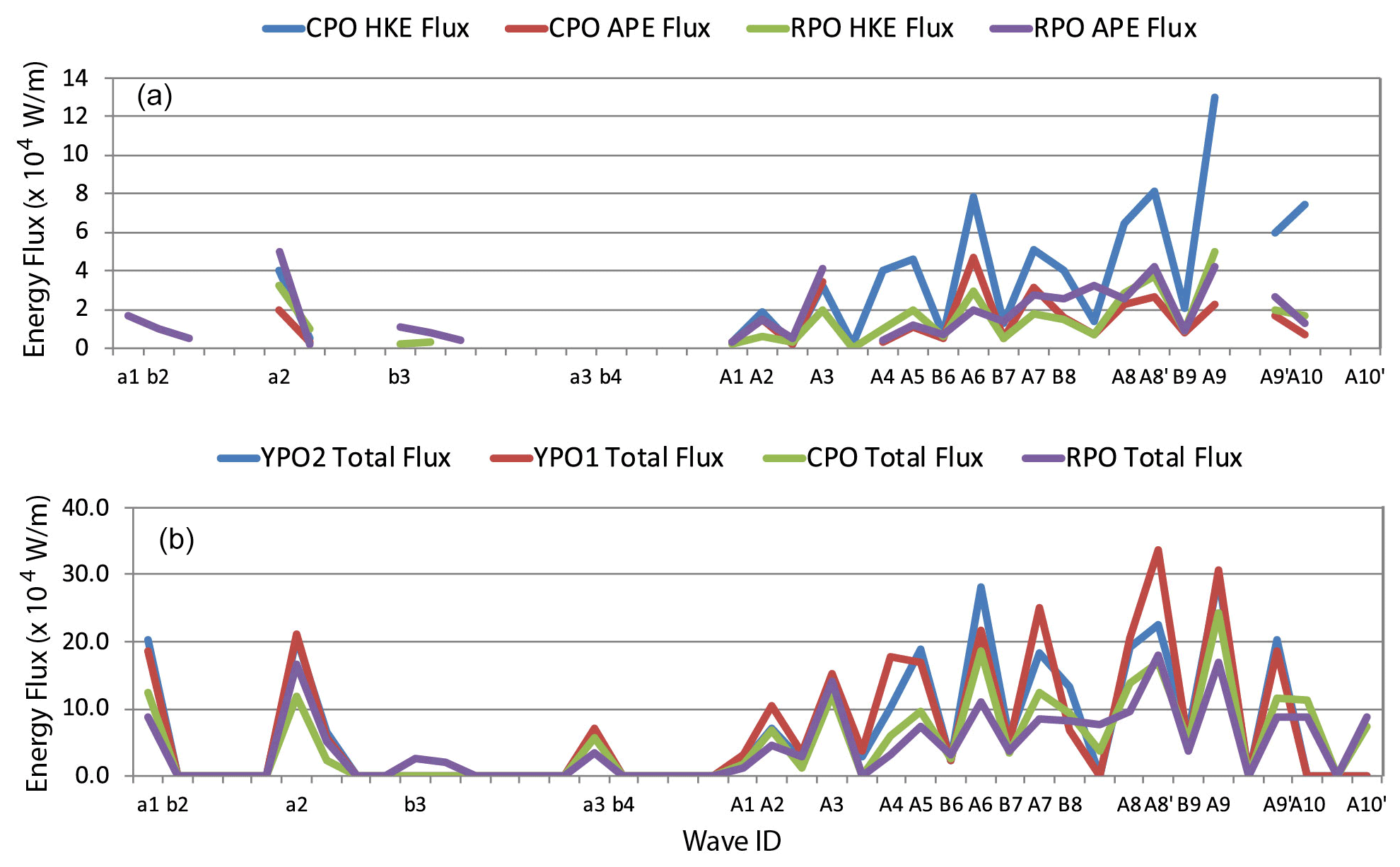
Figure 16The energy fluxes up the slope for each of the nonlinear internal waves identified in the sand dunes moored array data. (a) The kinetic and potential energy flux for moorings CPO and RPO. (b) The total energy flux for all four moorings. This is the sum of the kinetic, potential, and pressure work terms.
A conundrum remains the arrival of two large a waves with nearly equal amplitude separated by 2 h during the period of maximal tidal forcing, spring tide plus or minus 1 d. Additional work is needed to understand the origin of these waves.
At least two packet-generating mechanisms were clearly observed. Most a waves had already formed in the deep basin by the time they were incident upon the most offshore mooring, YPO2 at the 388 m isobath. The behavior of these waves depended on their amplitude: waves smaller than about 50 m and 100 MJ m−1 propagated adiabatically upslope with little change of form. Waves larger/more energetic than this formed packets via wave dispersion. Wave breaking was not observed at any time, with the possible exception of the largest wave that was steepening on the back side at the shallowest mooring, RPO at 266 m depth. The waves likely break, and/or reflect, inshore of 266 m, where the bottom is also steeper. On the other hand, some of the b waves were incident on YPO2, while others were absent at YPO2 and formed while the internal tide shoaled between YPO2 and RPO. These waves and wave packets were formed by the breaking of the leading, strongly convergent edge of the upslope-propagating internal tide (not to be confused with a breaking NLIW). This process took place near mooring CPO on the 342 m isobath. This process occurred just once per day and was most easily discerned by the downslope tidal current near the bottom, which was not complicated by upper ocean processes.
The energy transformations also depended on wave amplitude. For the smaller waves (E<100 MJ m−1), the incident APE was greater than the HKE and continued to grow upslope. For the larger waves, the incident HKE was larger than the APE, but the flux of HKE decreased sharply upslope, especially between 342 and 266 m, while the flux of APE in that depth range increased slightly, resulting in greater APE than HKE farther onshore. These results are in rough agreement with recent theory and numerical simulations of shoaling waves.
With the possible exception of one (largest) wave, no breaking NLIWs were observed anywhere in the moored array. This is because neither of the criteria for breaking waves was met: the orbital velocities never exceeded the propagation speed, and wave amplitudes were too small. This situation contrasts with a similar depth range farther southwest, where larger waves were already actively breaking at the 300 m isobath. The more periodic, less turbulent environment presented to the subaqueous sand dune field may be relevant to its formation location along the slope. This and other forcing factors will be taken up in more detail in a subsequent work.
The HDFLook and GMT software used to create Fig. 9 is publicly available and may be found at https://hdfeos.org/software/HDFLook.php (Gonzalez and Deroo, 2008) and https://www.generic-mapping-tools.org/ (Wessel et al., 2019) respectively.
All data used in this paper including temperature, salinity, and velocity are available in the Meldeley Data Repository and may be accessed via https://doi.org/10.17632/6wwv4m4r97.1 (Bahr et al., 2022). This is an open link available to all. The raw image data for Fig. 9 are also publicly available from the NASA website at https://ladsweb.modaps.eosdis.nasa.gov/ (Wolfe, 2022).
SRR is the lead author and wrote the manuscript in its entirety. He also helped plan the experiment, participated in the cruises, and supplied a portion of the moored equipment. YJY is the lead scientist from Taiwan. He helped plan the experiment, participated in the work at sea, and supplied a portion of the equipment. He also arranged for the ship time and provided liaison with the Institute of Oceanography, National Taiwan University, and the Taiwanese government. CSC helped plan the experiment, participated in the cruises, and supplied a portion of the equipment, especially the acoustics gear. DBR helped plan the experiment, participated in the cruises, and supplied some of the equipment, most notably the acoustics gear. FLB is an oceanographer and computer programmer, who conducted the data downloading, processing, and quality control for most of the instruments deployed. He also produced most of the figures that appear in the paper.
The contact author has declared that neither they nor their co-authors have any competing interests.
Publisher’s note: Copernicus Publications remains neutral with regard to jurisdictional claims in published maps and institutional affiliations.
This article is part of the special issue “Nonlinear internal waves”. It is not associated with a conference.
Wen-Hwa Her (IONTU) and Marla Stone (NPS) led the mooring work at sea. We thank the officers and crew of the research vessels OCEAN RESEARCHER 1, OCEAN RESEARCHER 3, and OCEAN RESEARCHER 5.
This research has been supported by the Office of Naval Research (grant no. N000141512464) and the Ministry of Science and Technology, Taiwan.
This paper was edited by Marek Stastna and reviewed by Peter Diamessis and one anonymous referee.
Alford, M. H., Lien, R.-C., Simmons, H., Klymak, J., Ramp, S. R., Yang, Y.-J., Tang, T.-Y., Farmer, D., and Chang, M.-H.: Speed and evolution of nonlinear internal waves transiting the South China Sea, J. Phys. Oceanogr., 40, 1338–1355, 2010.
Alford, M. H., MacKinnon, J. A., Nash, J. D., Simmons, H., Pickering, A., Klymak, J. M., Pinkel, R., Sun, O., Rainville, L., Musgrave, R., Beitzel, T., Fu, K.-H., and Lu, C.-W.: Energy flux and Dissipation in Luzon Strait: Two tales of two ridges, J. Phys. Oceanogr. 41, 2211–2222, 2011.
Alford, M. H., Peacock, T., MacKinnon, J. A. et al.: The formation and fate of internal waves in the South China Sea, Nature, 521, 65–69, 2015.
Bahr, F., Ramp, S., Yang, Y. J.: Observations of shoaling internal wave transformation over a gentle slope in the South China Sea, V1, Mendeley Data [data set], https://doi.org/10.17632/6wwv4m4r97.1, 2022.
Buijsman, M. C., Kanarska, Y., and McWilliams, J. C.: On the generation and evolution of nonlinear internal waves in the South China Sea, J. Geophys. Res.-Oceans, 115, C02012, https://doi.org/10.1029/2009JC005275, 2010a.
Buijsman, M. C., McWilliams, J. C., and Jackson, C. R.: East-west asymmetry in nonlinear internal waves from Luzon Strait, J. Geophys. Res.-Oceans, 115, C1057, https://doi.org/10.1029/2009JC006004, 2010b.
Chang, M.-H., Lien, R.-C., Tang, T. Y., D'Asaro, E. A., and Yang, Y. J.: Energy flux on nonlinear internal waves in the northern South China Sea, Geophys. Res. Let., 33, L03607, https://doi.org/10.1029/2005GL025196, 2006.
Chang, M.-H., Lien, R.-C., Lamb, K. G., and Diamessis, P. J.: Long-term observations of shoaling internal solitary waves in the northern South China Sea, J. Geophys. Res.-Oceans, 126, e2020JC017129, https://doi.org/10.1029/2020JC017129, 2021a.
Chang, M.-H., Cheng, Y.-H., Yang, Y.-J., Jan, S., Ramp, S. R., Reeder, D. B., Hseih, W.-T., Ko, D. S., Davis, K. A., Shao, H.-J., and Tseng, R.-S.: Direct measurements reveal instabilities and turbulence within large amplitude internal solitary waves beneath the ocean, Communications Earth & Environments, 2, 15, https://doi.org/10.1038/S43247-020-00083-6, 2021b.
Chen, Y.-J., Ko, D. S., and Shaw, P.-T.: The generation and propagation of internal solitary waves in the South China Sea, J. Geophys. Res.-Oceans, 118, 6578–6589, https://doi.org/10.1002/2013JC009319, 2013.
Chiu, L. Y. S. and Reeder, D. B.: Acoustic mode coupling due to subaqueous sand dunes in the South China Sea, J. Acoust. Soc. Am., 134, EL198, https://doi.org/10.1121/1.4812862, 2013.
Chiu, L. Y. S., Chang, A. Y. Y., and Reeder, D. B.: Resonant interaction of acoustic waves with subaqueous bedforms: Sand dunes in the South China Sea, J. Acoust. Soc. Am., 138, EL515, https://doi.org/10.1121/1.4937746, 2015.
Du, T., Tseng, Y.-H., and Yan, X.-H.: Impacts of tidal currents and Kuroshio intrusion on the generation of nonlinear internal waves in Luzon Strait, J. Geophys. Res.-Oceans, 113, C08015, https://doi.org/10.1029/2007JC004294, 2008.
Duda, T. F., Lynch, J. F., Irish, J. D., Beardsley, R. C., Ramp, S. R., Chiu, C.-S., Tang, T.-Y., and Yang, Y.-J.: Internal tide and nonlinear internal wave behavior at the continental slope in the northern South China Sea, IEEE J. Oceanic Eng., 29, 1105–1131, 2004.
Egbert, G. and Erofeeva, S.: Efficient inverse modeling of barotropic ocean tides, J. Atmos. Ocean. Tech., 19, 183–204, 2002.
Farmer, D., Li, Q., and Park, J.-H.: Internal wave observations in the South China Sea: The role of rotation and non-linearity, Atmos.-Ocean, 47, 267–280, 2009.
Farmer, D. M., Alford, M. H., Lien, R.-C., Yang, Y. J., Chang, M.-H., and Li, Q.: From Luzon Strait to Dongsha Plateau: Stages in the life of an internal wave, Oceanography, 24, 64–77, 2011.
Gonzalez, L. and Deroo, C.: Manuel HDFLook/HDFLook MODIS, Laboratoire d’Optique Atmospherique, Universite de Lille, France [software], https://hdfeos.org/software/HDFLook.php (last access: June 2014), 2008.
Grimshaw, R., Pelinovsky, E. N., Talipova, T. G., and Kurkina, A.: Simulations of the transformation of internal solitary wave on oceanic shelves, J. Phys. Oceanogr., 34, 2774–2791, 2004.
Grimshaw, R., Guo, C., Helfrich, K., and Vlasenko, V.: Combined effect of rotation and topography on shoaling oceanic internal solitary waves, J. Phys. Oceanogr., 44, 1116–1132, 2014.
Helfrich, K. R.: Internal solitary wave breaking and run-up on a uniform slope, J. Fluid Mech., 243, 133–154, 1992.
Helfrich, K. R. and Melville, W. K.: On long nonlinear internal waves over slowly varying topography, J. Fluid Mech., 149, 305–317, 1986.
Helfrich, K. R., Trowbridge, J. H., and Reeder, D. B.: High dissipation of an internal solitary wave over sand dunes, J. Phys. Oceanogr., in review, 2022.
Hsu, M.-K. and Liu, A. K.: Nonlinear internal waves in the South China Sea, Can. J. Remote Sens., 26, 72–81, 2000.
Jackson, C. B.: An empirical model for estimating the geographic location of nonlinear internal solitary waves, J. Atmos. Ocean. Tech., 26, 2243–2255, 2009.
Klymak, J. M., Pinkel, R., Liu, C.-T., Liu, A. K., and David, L.: Prototypical solitons in the South China Sea, Geophys. Res. Lett., 33, L11607, https://doi.org/10.1029/2006GL025932, 2006.
Kunze, E., Rosenfeld, L. K., Carter, G. S, and Gregg, M. C.: Internal waves in Monterey Submarine Canyon, J. Phys. Oceanogr., 32, 1890–1913, 2002.
Lamb, K. G.: A numerical investigation of solitary internal waves with trapped cores formed via shoaling, J. Fluid Mech., 451, 109–144, 2002.
Lamb, K. G. and Nguyen, V. T.: Calculating energy flux in internal solitary waves with an application to reflectance, J. Phys. Oceanogr., 39, 559–580, 2009.
Lamb, K. G. and Warn-Varnas, A.: Two-dimensional numerical simulations of shoaling internal solitary waves at the ASIAEX site in the South China Sea, Nonlin. Processes Geophys., 22, 289–312, https://doi.org/10.5194/npg-22-289-2015, 2015.
Lee, C. M, Kunze, E., Sanford, T. B., Nash, J. D., Merrifield, M. A., and Holloway, P. E.: Internal tides and turbulence along the 3000-m isobath of the Hawaiian Ridge, J. Phys. Oceanogr., 36, 1165–1183, 2006.
Li, Q. and Farmer, D. M.: The generation and evolution of nonlinear internal waves in the deep basin of the South China Sea, J. Phys. Oceanogr., 41, 1345–1363, 2011.
Lien, R. C., D'Asaro, E. A., Henyey, F., Chang, M. H., Tang, T. Y., and Yang, Y.-J.: Trapped core formation within a shoaling nonlinear internal wave, J. Phys. Oceanogr., 42, 511–525 2012.
Lien, R. C., Henyey, F., Ma, B., and Yang, Y. J.: Large-amplitude internal solitary waves observed in the northern South China Sea: Properties and Energetics, J. Phys. Oceanogr., 44, 1095–1115, 2014.
Liu, A. K., Ramp, S. R., Zhao, Y., and Tang, T. Y.: A case study of internal solitary wave propagation during ASIAEX 2001, IEEE J. Oceanic Eng., 29, 1144–1156, 2004.
Moum, J. N., Klymak, J. M., Nash, J. D., Perlin, A., and Smyth, W. D.: Energy transport by nonlinear internal waves, J. Phys. Oceanogr., 37, 1968–1988, 2007.
Nash, J. D., Alford, M. H., and Kunze, E.: Estimating internal wave energy fluxes in the ocean, J. Atmos. Ocean. Tech., 22, 1551–1570, 2005.
Nash, J. D., Kunze, E., Lee, C. M., and Sanford, T. B.: Structure of the baroclinic tide generated at Kaena Ridge, Hawaii, J. Phys. Oceanogr., 36, 1123–1135, 2006.
Nash, J. D., Kelly, S. M., Shroyer, E. L., Moum, J. N., and Duda, T. F.: The unpredictable nature of internal tides on the continental shelf, J. Phys. Oceanogr., 42, 1981–2000, 2012.
Orr, M. H. and Mignerey, P. C.: Nonlinear internal waves in the South China Sea: Observations of the conversion of depression internal waves to elevation internal wages, J. Geophys. Res. 108, 3064, https://doi.org/10.1029/2001JC001163, 2003.
Ramp, S. R., Chiu, C. S., Kim, H.-R., Bahr, F. L., Tang, T.-Y., Yang, Y. J., Duda, T., and Liu, A. K.: Solitons in the Northeastern South China Sea Part I: Sources and Propagation Through Deep Water, IEEE J. Oceanic Eng., 29, 1157–1181, 2004.
Ramp, S. R., Yang, Y. J., and Bahr, F. L.: Characterizing the nonlinear internal wave climate in the northeastern South China Sea, Nonlin. Processes Geophys., 17, 481–498, https://doi.org/10.5194/npg-17-481-2010, 2010.
Ramp, S. R., Park, J.-H., Yang, Y. J., Bahr, F. L., and Jeon, C.: Latitudinal Structure of Solitons in the South China Sea, J. Phys. Oceanogr., 49, 1747–1767, 2019.
Ramp, S. R., Yang, Y.-J., Jan, S., Chang, M.-H., Davis, K. A., Sinnett, G., Bahr, F. L., Reeder, D. B., Ko, D. S., and Pawlak, G.: Solitary waves impinging on an isolated tropical reef: Arrival patterns and wave transformation under shoaling, J. Geophys. Res.-Oceans, 127, e2021JC017781, https://doi.org/10.1029/2021JC017781, 2022.
Reeder, D. B., Ma, B., and Yang, Y. J.: Very large subaqueous sand dunes on the upper continental slope in the South China Sea generated by episodic, shoaling deep-water internal solitary waves, Mar. Geol., 279, 12–18, 2011.
Rivera-Rosario, G., Diamessis, P. J., Lien, R.-C., Lamb, K. G., and Thomsen, G. N.: Formation of recirculating cores in convectively breaking internal solitary waves of depression shoaling over gentle slopes in the South China Sea, J. Phys. Oceanogr., 50, 1137–1157, https://doi.org/10.1175/jpo-d-19-0036.1, 2020.
Scotti, A., Beardsley, R. C., and Butman, B.: On the interpretation of energy and energy fluxes of nonlinear internal waves: An example from Massachusetts Bay, J. Fluid Mech., 561, 103–112, 2006.
Small, J.: A nonlinear model of the shoaling and refraction of interfacial solitary waves in the ocean. Part I: Development of the model and investigations of the shoaling effect, J. Phys. Oceanogr., 31, 3163–3183, 2001a.
Small, J.: A nonlinear model of the shoaling and refraction of interfacial solitary waves in the ocean. Part II: Oblique refraction across a continental slope and propagation over a seamount, J. Phys. Oceanogr., 31, 3184–3199, 2001b.
Turkington, B., Eydeland, A., and Wang, S.: A computatioinal method for solitary internal waves in a continuously stratified fluid, Stud. Appl. Math., 85, 93–127, 1991.
Vlasenko, V. and Hutter, K.: Numerical experiments on the breaking of solitary internal waves over a slope-shelf topography, J. Phys. Oceanogr., 32, 1779–1793, 2002.
Vlasenko, V. and Stashchuk, N.: Three-dimensional shoaling of large-amplitude internal waves, J. Geophys. Res.-Oceans, 112, C11018, https://doi.org/10.1029/2007JC004107, 2007.
Vlasenko, V., Ostrovsky, V. L., and Hutter, K.: Adiabatic behavior of strongly nonlinear internal solitary waves in slope-shelf areas, J. Geophys. Res., 110, C04006, https://doi.org/10.1029/2004JC002705, 2005.
Wessel, P., Luis, J. F., Uieda, L., Scharroo, R., Wobbe, F., Smith, W. H. F., and Tian, D.: The Generic Mapping Tools version 6, Geochem. Geophys. Geosy., 20, 5556–5564, https://doi.org/10.1029/2019GC008515, 2019 (software available at: https://www.generic-mapping-tools.org/, last access: June 2014).
Wolfe, R.: Level-1 and Atmosphere Archive and Distribution System (LAADS) Distributed Active Archive Center (DAAC), NASA Goddard Space Flight Center, Greenbelt, Maryland [data set], https://ladsweb.modaps.eosdis.nasa.gov/ (last access: June 2014), 2022.
Yang, Y. J., Fang, Y. C., Chang, M.-H., Ramp, S. R., Kao, C.-C., and Tang, T.-Y.: Observations of second baroclinic mode internal solitary waves on the continental slope of the northern South China Sea, J. Geophys. Res.-Oceans, 114, C10003, https://doi.org/10.1029/2009JC005318, 2009.
Yang, Y. J., Fang, Y. C., Tang, T. Y., and Ramp, S. R.: Convex and concave types of second baroclinic mode internal solitary waves, Nonlin. Processes Geophys., 17, 605–614, https://doi.org/10.5194/npg-17-605-2010, 2010.
Zhang, Z., Fringer, O. B., and Ramp, S. R.: Three-dimensional, nonhydrostatic numerical simulation of nonlinear internal wave generation and propagation in the South China Sea, J. Geophys. Res.-Oceans, 116, C05022, https://doi.org/10.1029/2010JC006424, 2011.