the Creative Commons Attribution 4.0 License.
the Creative Commons Attribution 4.0 License.
 | 05 Jul 2022
Predicting sea surface temperatures with coupled reservoir computers
Benjamin Walleshauser
Erik Bollt
Sea surface temperature (SST) is a key factor in understanding the greater climate of the Earth, and it is also an important variable when making weather predictions. Methods of machine learning have become ever more present and important in data-driven science and engineering, including in important areas for Earth science. Here, we propose an efficient framework that allows us to make global SST forecasts using a coupled reservoir computer method that we have specialized to this domain, allowing for template regions that accommodate irregular coastlines. Reservoir computing is an especially good method for forecasting spatiotemporally complex dynamical systems, as it is a machine learning method that, despite many randomly selected weights, is highly accurate and easy to train. Our approach provides the benefit of a simple and computationally efficient model that is able to predict SSTs across the entire Earth's oceans. The results are demonstrated to generally follow the actual dynamics of the system over a forecasting period of several weeks.
- Article
(1486 KB) - Full-text XML
- BibTeX
- EndNote


As most of Earth's surface is covered by water, global sea surface temperatures (SSTs) are an important parameter in understanding the greater climate of the Earth. The SST is an important variable in the study of marine ecology (Gomez et al., 2020; Novi et al., 2021), weather prediction (Dado and Takahashi, 2017) and to help project future climate scenarios (Pastor, 2021). However, the task of predicting changes in the SST is quite difficult due to large variations in heat flux, radiation and diurnal wind near the surface of the sea (Patil et al., 2016).
Given the importance of the SST to the fuller Earth weather and climate system, there is significant interest in forecasting this spatiotemporally complex process. Methods for predicting changes in the SST can be divided into two different categories: numerical methods and data-driven methods. Numerical methods are based on the underlying knowledge of the governing physics behind the system and the simulation thereof. These are widely used to predict SST over a large area (Stockdale et al., 2006; Krishnamurti et al., 2006). However, data-driven methods encompass statistical and machine learning approaches, and they are widely used to predict the SST, often with little to no knowledge regarding the relevant physical principles behind the dynamics of the system, thereby reducing the complexity of the model. Several statistical methods that have been used include Markov models (Xue and Leetmaa, 2000; Johnson et al., 2000), linear regression (Kug et al., 2004) and empirical canonical correlation analysis (Collins et al., 2004). Meanwhile machine learning methods have included techniques such as support vector machines (SVMs; Lins et al., 2013), long short-term memory neural networks (LSTMs; Zhang et al., 2017; Kim et al., 2020; Xiao et al., 2019a) and memory graph convolutional networks (MGCNs; Zhang et al., 2021). In this paper, we utilize coupled reservoir computers (RCs), thereby taking advantage of the reduced complexity of data-driven methods while still being able to predict temperatures globally due to the minimal training required by each RC. We have adapted the RC concept for spatiotemporal processes to allow for coupled local templates that accommodate the peculiarities associated with varying coastlines.
Reservoir computers have been shown to be excellent at predicting complex dynamical systems (Ghosh et al., 2021; Pandey and Schumacher, 2020), regardless of the relative simplicity of the approach. They have even been shown to be proficient in the prediction of spatiotemporally complex systems, such as the Kuramoto–Sivashinsky partial differential equation (Vlachas et al., 2020) and cell segmentation (Hadaeghi et al., 2021). In our case, the use of coupled reservoir computers is introduced due to the large number of points on the map, making it computationally challenging to utilize a single large reservoir computer. The reservoirs are coupled together by making the reservoirs functions of points outside their forecast domain, effectively creating overlap.
Reservoir computing is a type of recurrent neural net where the only layer trained is the output layer; this is done with a simple linear method. Compared with traditional recurrent neural networks, reservoir computers utilize randomly generated input and middle weights, which, in effect, reduces training time significantly. The reservoir computer is stated as follows (Jaeger and Haas, 2004):
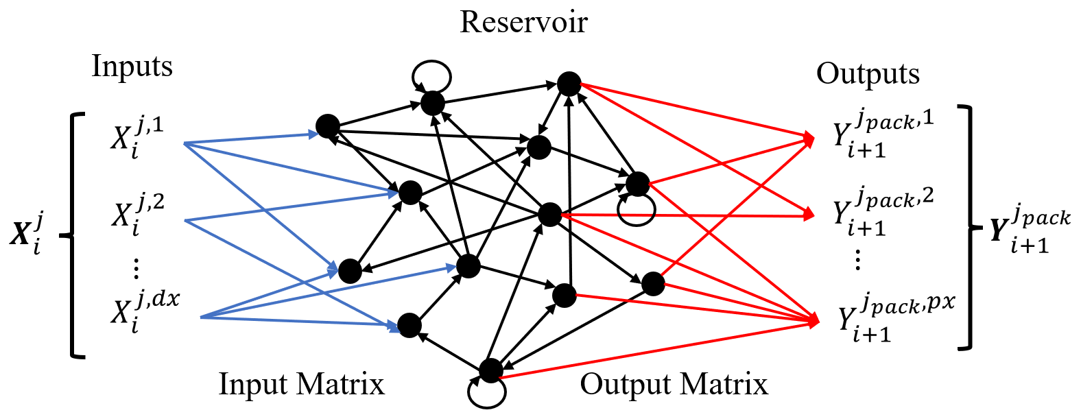
The inputs Xi (of total length dx) represent the raw data which describe a system; in our case, these would be the temperatures at points in the sea. These are fed into the reservoir via the input matrix Win, which has weights that are determined via sampling a uniform distribution . The reservoir dimension N describes how many nodes there are to be within the reservoir. Therefore, in order to transform the inputs into the space of the reservoir, the dimensions of Win will be N×dx.
The reservoir state r, which evolves according to Eq. (1), carries information about the current and previous states of the system. During training, the reservoir states are horizontally concatenated as time evolves to form the matrix , where ttrain is the number of data points being used to train the model and, thus, the computational complexity associated with the matrix operations stated in Eq. (2). The dimensions of R at the end of the training phase will then be N×ttrain.
The reservoir matrix A, which contains the middle weights, is a sparse matrix with a set density d, with nonzero values that are sampled from a uniform distribution . The matrix A will have dimensions of N×N, corresponding to the N reservoir nodes. The spectral radius ρ of A is an important metaparameter in the formation of the RC (Jiang and Lai, 2019), and it can be adjusted by scaling A (which essentially just involves changing β). The activation function q(s) is usually picked to be a nonlinear function such as the sigmoid function or the hyperbolic tangent function. Often, a bias term b is included when one desires to shift the activation function a set amount. After the training dataset is cycled through and the matrix R is completed, the output matrix Wout is then found via a ridge regression:
which utilizes the identity matrix I scaled by a regularization parameter λ to prevent overfitting. As the output matrix is transforming reservoir states to a desired output Yi+1 (of length px), the dimension of Wout will be px×N. The trained model can then be used to forecast autonomously by inserting the newly predicted values Yi+1 back into the reservoir on the next iteration as Xi.
As we would like to predict the SST across the entire globe, it is computationally challenging to use a single reservoir computer to forecast for the entire map due to the number of points on the map. From the dataset, there will be a total of n⋅m points on the map. If we were to use a single reservoir computer, the size of the input dataset Xi would be around (as 71 % of the Earth's surface is water) for each time step. It will be seen in Sect. 4 that the values of n and m that are ultimately used to train our model are 120 and 240, respectively; hence, the total number of points that are not on land across the map is about 20 448. Thus, even if the reservoir dimension N is 15:1 with respect to the size of the input dataset (which is relatively small; e.g., the value of N commonly used for the 3D Lorenz system is 1000; Bollt, 2021), the size of the resulting matrix A would be 306 720×306 720, which, assuming each element requires 8 B, would require 750 GB to store.
Therefore, in this application, it is better to follow the methodology laid out by Pathak et al. (2018) to model the evolution of the SST with the use of smaller reservoir computers that each cover a small domain of the map. This approach is advantageous because the input and middle weights for a reservoir computer are chosen randomly, thereby allowing us to reuse the same input matrices1 Win and the same reservoir matrix A between the individual RCs. Now, each individual RC learns the local behavior of the points within its forecasting domain (defined as a pack) while still being connected to the global system via coupling with its neighbors.
A pack is essentially a collection of contiguous indices on the greater map that will be assigned to a given RC. In other words, a pack is an RC model of the dynamics, for a local region of the globe, that is designed to accommodate any local peculiarities of the land–water interface and also couples into other neighboring packs. This reservoir computer will then be solely responsible for predicting the temperatures within its pack as time evolves. For simplicity's sake, in this study, points within a pack are grouped in the shape of rectangles, where the number of rows of points within the pack is defined as npack and the number of columns subsequently mpack. Therefore, each RC will be responsible for forecasting a maximum of npack⋅mpack spatial points on the map. As there are n⋅m total points on the map, the number of RCs needed will then be . An illustration of the various packs on a sample map are provided in Fig. 1.
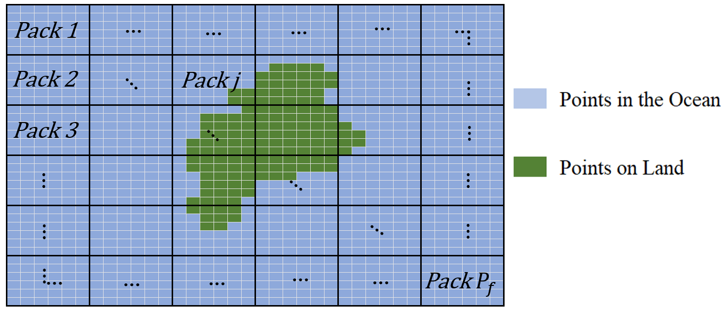
Figure 1The various packs on a sample map. The points within a pack that are blue are the eligible points in the ocean that the pack’s designated reservoir computer will attempt to forecast. Points in green represent land, which are not eligible points and whose indices are ignored in the formation of the pack.
No points containing land are assigned to a RC; therefore, some packs will have more or less points than others, due to these points on land. It should also be noted that no point on the map can be in more than one pack, as packs do not overlap. The SSTs of the points within the jth pack at the ith day are stacked in the vector , which is of length px:
For the various reservoirs to interact with one another, coupling is introduced by including the SST of the neighbors surrounding a pack. The neighbors of a pack are the non-land points that are either directly touching or are on the corner of a point within the pack. As many points within a pack share similar neighbors, only unique neighbors are kept, and their SSTs at the ith day are compiled into the vector . The neighbors for a given pack on the sample map are illustrated below in Fig. 2.
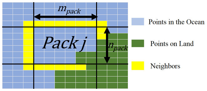
Figure 2Illustration of the jth pack with its valid neighbors denoted by a yellow highlight. In this example, it is evident that px is equal to 32 (number of pack points in the ocean) and dx is equal to 54 (px plus the number of neighbors). It is also evident that npack and mpack are both equal to 6 in this case.
The vectors and are combined to form the vector (of length dx), which contains all of the SSTs for the pack and its neighbors at the ith day and is ultimately the input for the jth reservoir computer.
As we would like the model to predict SSTs within the pack at the next day , the reservoir computer for the jth pack can now be written as follows:
Each reservoir computer is trained over the entire training dataset from d. Each pack contains a distinct output matrix , such that the reservoir states are matched with the values of the SST within the pack at the next day. In order to save computer memory, it is advisable to create an array of input matrices with values of dx from 1 to and then assign these to RCs with a similar value of dx, denoted by . One middle-weight matrix A is shared between all of the RCs, as the reservoir dimension N is set to be fixed between all of the reservoirs. The architecture of a single reservoir computer is described in Fig. 3.
The dataset from the Group for High Resolution Sea Surface Temperature (GHRSST) used to train and validate the model is titled “GHRSST Level 4 MUR 0.25 deg Global Foundation Sea Surface Temperature Analysis (v4.2)”; it contains SST data in degrees kelvin on a global 0.25∘ grid from 2002 to 2021 in 1 d increments. This version is based on nighttime GHRSST L2P skin and sub-skin SST observations from several instruments and is publicly available online via the Physical Oceanography Distributed Active Archive Center (PO.DAAC, 2019). The data were downloaded with the use of OPeNDAP on 10 October 2021.
The years 2003 to 2020 of the dataset were selected to form the training and validation dataset. The data are given in an equirectangular format, which is used throughout the modeling process for simplification purposes, even though this consequentially leads to a more refined mesh near the poles. The time series data were split into a training and validation dataset, consisting of 6533 and 42 d, respectively. We choose not to normalize the data, as the data are univariate and the reservoir state is effectively scale-free, with scale being reintroduced with the trained output matrix.
In order to reduce the number of spatial points within the dataset, the data were discretized such that the SST was now on a global 1.5∘ degree grid. This was performed by grouping original data points in a 6×6 matrix and then taking the average over the group. If a grouping contained a point on land, this value was ignored in the computation of the average of the group. Therefore, the dataset for a given day went from a 720×1440 to a 120×240 dataset; hence, n=120 and m=240.
To subsequently forecast the global SST with the trained model, two different prediction types are performed. To begin testing the short-term accuracy of the model, daily predictions are performed over the course of 6 weeks. The actual values of the SST are fed as inputs into the reservoir during this time period, and the predicted values for the next day are read out. This type of forecast has a real-world application in the form of filling in SST datasets when there is cloud cover or data corruption (Case et al., 2008), as the model can be used to estimate data for the missing days. Then, to test the long-term accuracy of the model, the model is allowed to run autonomously over the same 6 weeks. Now, the model is still predicting SST each day, but it only has access to its own previous prediction. This form of the forecast would be more applicable to weather prediction, as it could be coupled with an atmospheric model to help predict near-future weather patterns.
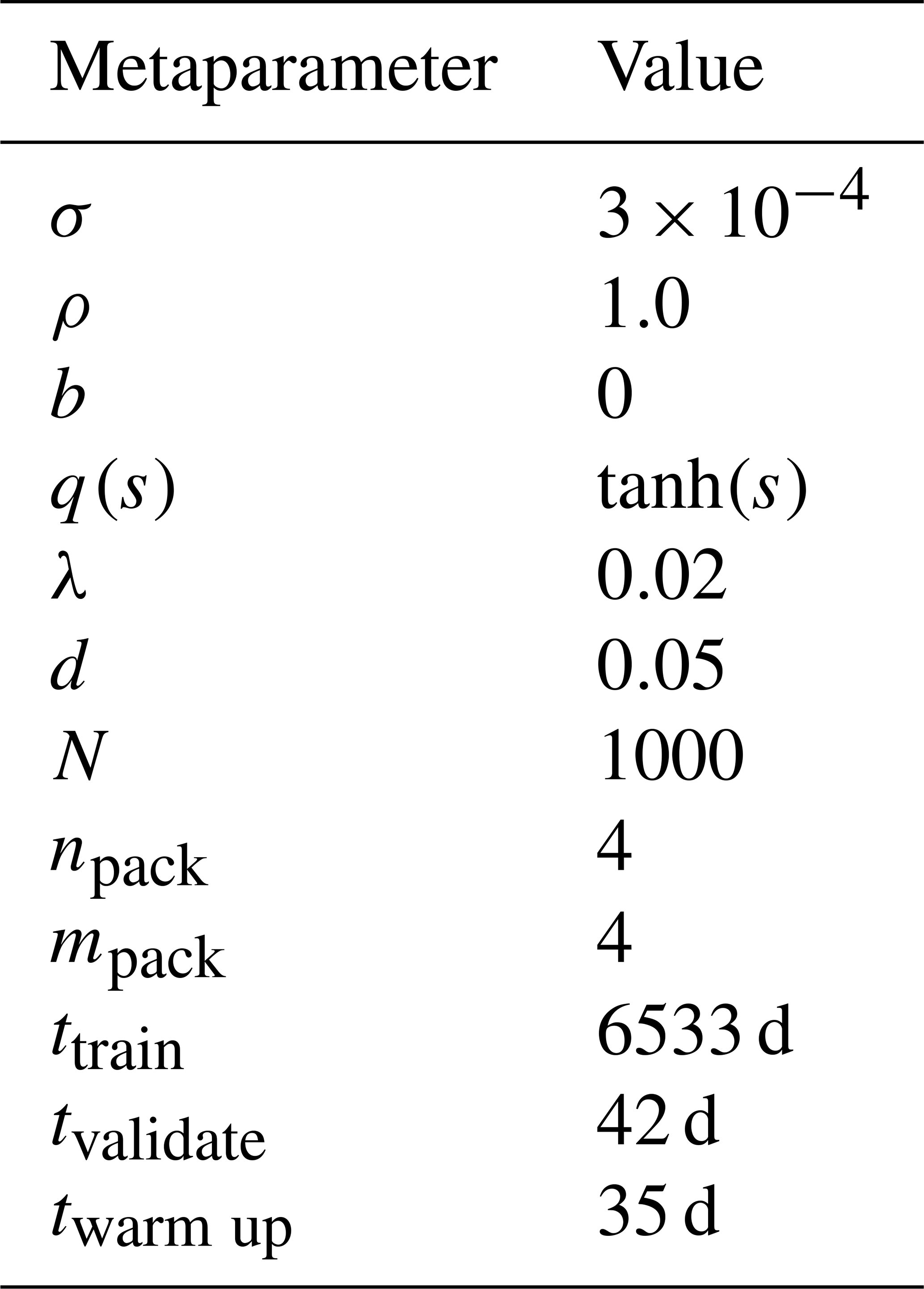
For both prediction types, the reservoir states are all cleared to zero prior to forecasting and then run over twarm up days prior to the validation time frame, thereby providing an initial condition for the model to begin from. Via cross validation, several metaparameters (σ, N and twarm up) were optimized, and the values that were found to perform the best are described in Table 1. It was noticed that the results were not significantly increased for a value of twarm up greater than 35 d. Results did consistently improve with an increasing reservoir dimension N, leading us to choose the value N=1000. One of the more sensitive metaparameters was the value of σ, which was found to provide optimal results when it had a magnitude of the order of 10−4. In the spirit of simplicity, we choose not to rigorously optimize the remaining metaparameters; rather, we choose them based off of heuristics.
The model was implemented using the MATLAB R2019b platform, from a personal laptop, and the training time was slightly over 40 min. It is likely, given the embarrassingly parallelizable nature of this task, that an implementation that leverages GPU-style computation could speed this stage up considerably. To observe the effect of the random input and middle weights on the model, 15 different models are created that all have the same metaparameters as described in Table 1. Even though the model predicts SST across the entire Earth, several time series at points chosen arbitrarily are included in each section to locally validate the forecast, the coordinates of which can be found below in Table 2. In this local time series analysis, the forecasts from the 15 different models are averaged, and ±1 standard deviation in the predicted values is represented above and below the average value using a shaded outline.

To determine the quality of the forecast over the entire ocean, the mean absolute error (MAE), the root-mean-square error (RMSE) and the maximum error in the forecast for a given day across the entire map are found. To find the MAE in the forecast at a given day, a weighted average is performed on the error ei across the map, where ep,i denotes the absolute error at point p on the map at the ith day. We perform this weighting due to the mesh being more refined near the poles compared with points near the Equator; hence, the area attributable to a given point Ωp is not necessarily the same for other points. It should also be noted that we treat areas near the poles consisting of time-dependent sea ice simply as points within the ocean. The actual area encompassed by a given point was found by simply using MATLAB’s built in “areaquad” function. The MAE in the forecast across the map at the ith day is then given by Eq. (8), where k is the number of points on the map that lie in the ocean ().
Similarly, the RMSE on the ith day is then given by Eq. (9).
Finally, the maximum error is simply the largest error in the forecast across all points on the ith day. These error values are found for each of the 15 models every day in the forecasting period; subsequently, the average values and standard deviations between models are found to observe the effect of randomness.
5.1 Daily forecasts
Daily forecasting operates by continually inserting the actual SST of the previous day Xi into the reservoirs and then reading out the model prediction of the SST at the next day Yi+1, subsequently repeating this procedure over the course of the validation time frame. The time series for the forecasted SSTs at the 10 different points are provided below in Fig. 4 and are also matched with the actual SSTs each day in Fig. 5.
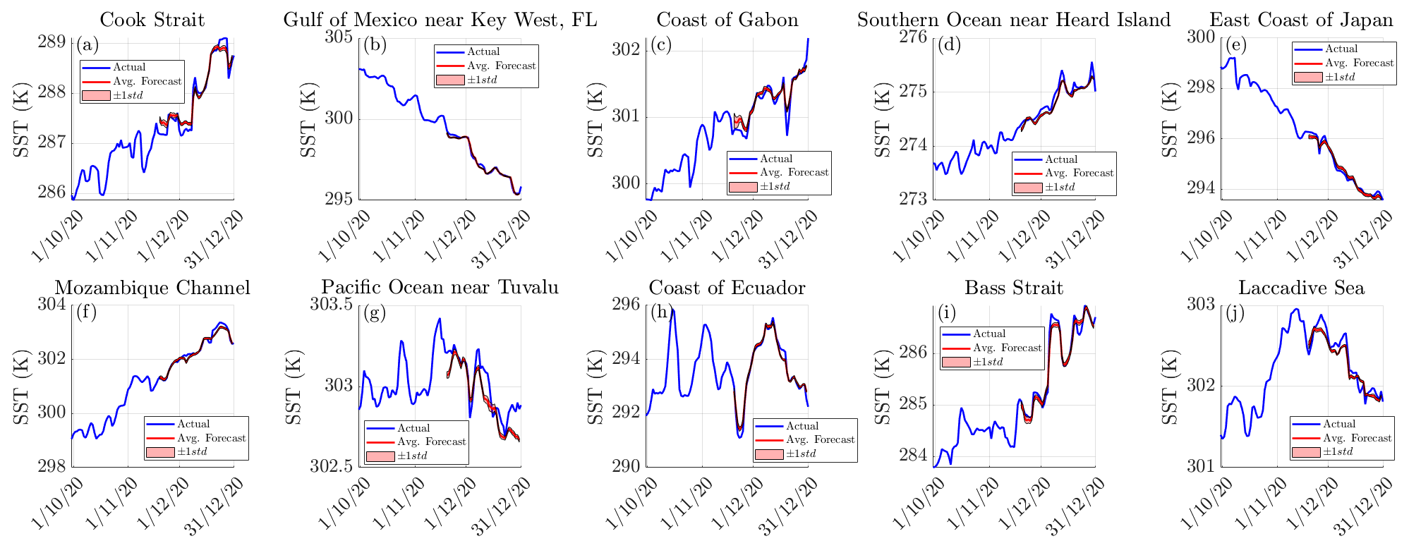
Figure 4The 1 d forecasts of the SST at various points in the ocean. The average forecasted SSTs and the true SSTs are represented by the red and blue lines, respectively. About the average there is a shaded outline representing ±1 standard deviation in the forecast between models, although it is not entirely evident due to all of models ultimately predicting similar values.
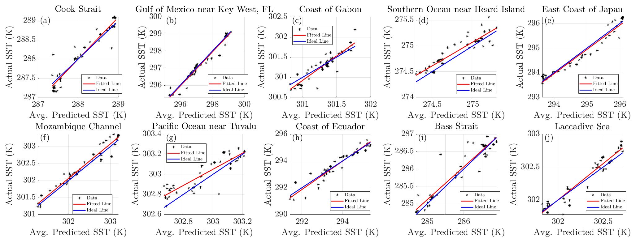
Figure 5The true SST compared to the average predicted SST, for the model predicting 1 d at a time. The red line indicates the resulting linear fit, and the blue line is the ideal place where the forecasted SSTs would match the true SSTs.
Table 3Regression statistics for the daily forecasts. Note that the slope m would ideally be equal to 1, the intercept b would be equal to 0 and the correlation coefficient r would be 1. Standard errors are provided for both m and b.
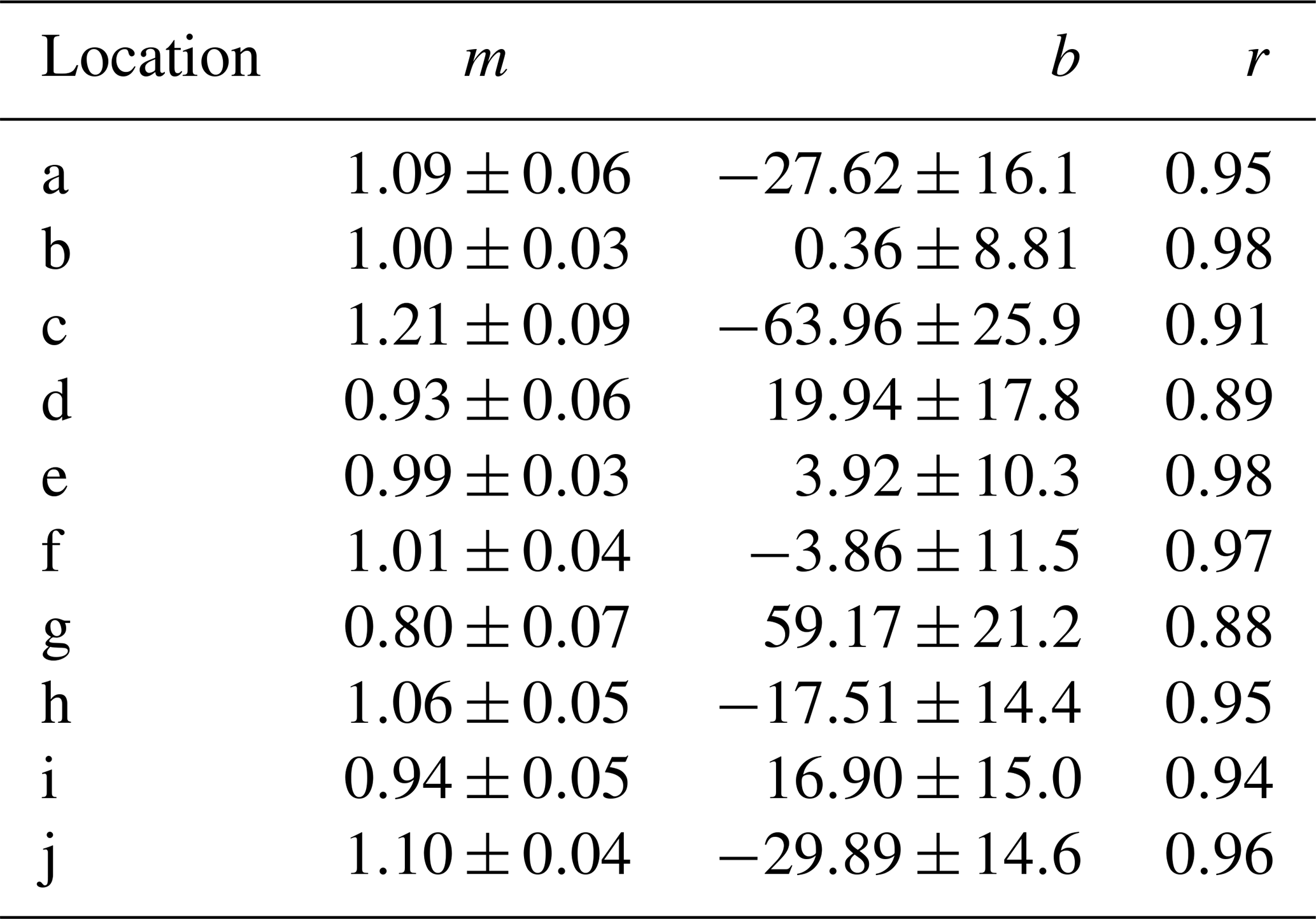
From Fig. 4, it is apparent that the forecasted SSTs closely follow the actual SSTs over the validation time frame for almost all locations. The model is seen to pick up on the changes in SST at locations where there is not a clear trend and the change in SST is seemingly chaotic, such as locations h, i and j, although there are some inaccuracies with the forecast at location g. There is also very little deviation between models, indicating that the effect of randomness on the model is practically negligible with regard to forecasting the daily SST. The correlation coefficients for the chosen sites are all 0.88 or greater, and the value of m is close to 1 (with minimal standard error) for most locations, indicating a strong relationship between the model's forecast and the actual values. To quantify how the model performs over the entire globe the MAE, RMSE and the maximum error for the daily forecasts are described below in Fig. 6.
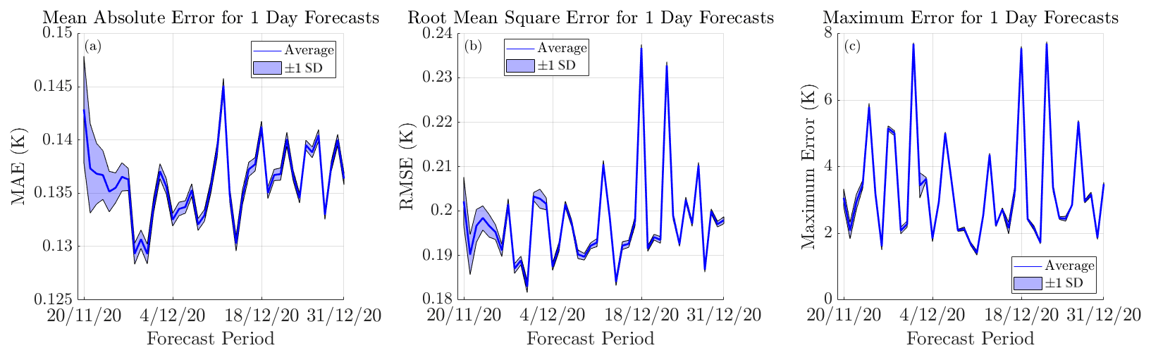
Figure 6The evolution of the error for the 1 d forecasts. The mean absolute error in the forecast over the entire ocean is depicted in panel (a), the root-mean-square is shown in panel (b) and the maximum error is presented in panel (c). The model average is represented using a dark blue line, and ±1 standard deviation is represented by the shaded outline above and below the average.
From Fig. 6, for each daily prediction, we see that the average MAE between models typically fluctuates between 0.13 and 0.15 K, the RMSE fluctuates between 0.18 and 0.24 K, and the maximum error fluctuates between 1 and 8 K. By calculating the mean of the model averages over the course of the 6-week forecasting period, we find that the model has as an average MAE of 0.136 K, an average RMSE of 0.197 K and an average maximum error of 3.308 K for a 1 d prediction horizon. For context, for a 1 d prediction horizon, Xiao et al. (2019b) reported a RMSE of 0.35 K for their forecast over the East China Sea with the use of a deep learning model constructed from ConvLSTM (convolutional long short-term memory) networks, and Shi et al. (2022) reported a RMSE of 0.241 K for their cyclic evolutionary network model forecasting over the South China Sea. It should also be noted that our error values typically do not decrease over the forecasting period, indicating that the chosen warm-up time of 35 d is sufficient, as there would be a decline in the error over time if the reservoir was gradually benefiting from more provided information.
5.2 The 6-week forecast
Meanwhile, for the 6-week forecast, the forecasted SSTs Yi+1 are input back into the reservoir on the next day, thereby taking the place of the actual SST Xi+1. This effectively allows the model to run autonomously over the validation time frame for a total of 42 d. The 10 time series for the forecasted SSTs are provided below in Fig. 7.
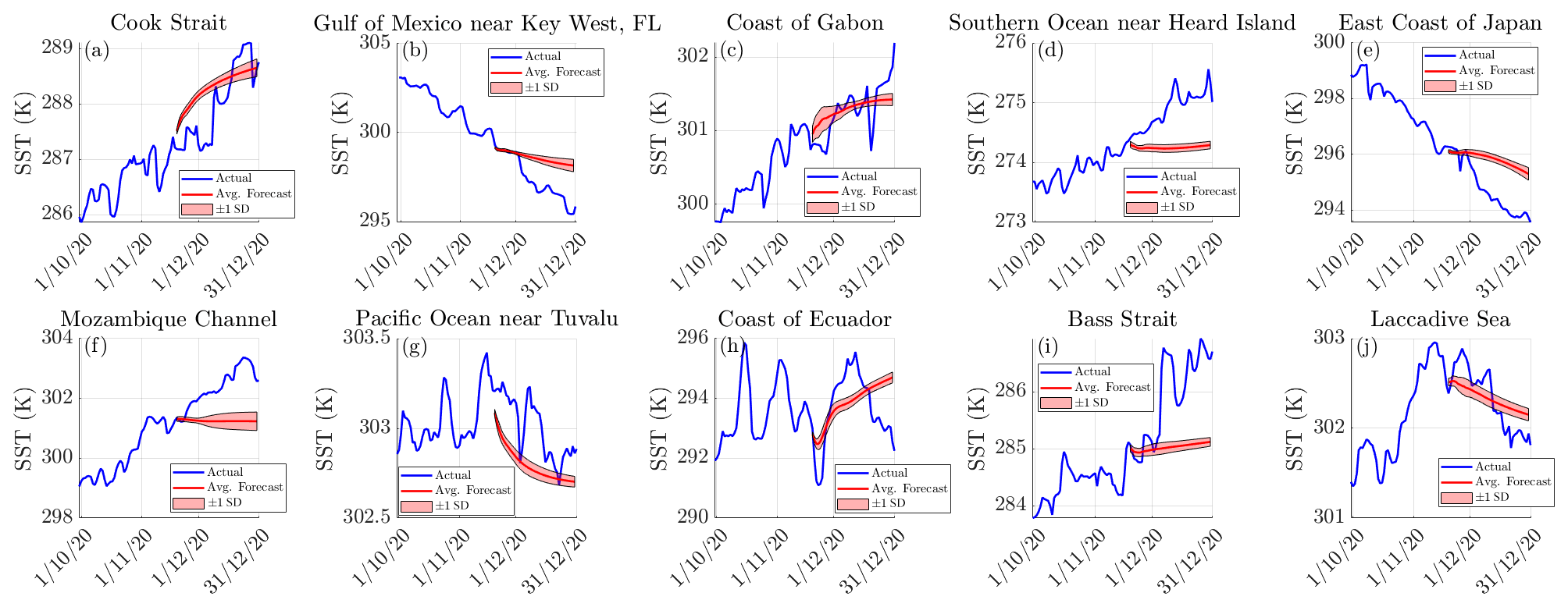
Figure 7Forecasted SSTs at various points in the ocean with the model running autonomously. The average forecasted SSTs and the actual SSTs are represented by the red and blue lines, respectively, with the shaded outline surrounding the average forecasted SSTs representing ±1 standard deviation in the forecast between the models.
From Fig. 7, it is apparent that the model typically predicts the general change in the SST for locations a, b, c, g, h and j. We find it especially impressive that the model is able to predict the cooling of the SST found at g and j and the warming at h. Meanwhile, the results for locations d, e and f are very poor given that the change in SST is fairly linear in the time leading up to the forecasting period and during it. The results at location i are also poor, as the model is unable to anticipate the rise in SST that began around the commencement of the forecasting period. These forecasts also depict how the intrinsic randomness of the model does play a slight role in the model output as time evolves, but it is an interesting feature that the standard deviation between models appears to reach a limit after several days of forecasting, as seen in Fig. 7d, e, g, h, i and j, and the standard deviation between models even decreases, as seen in Fig. 7c. To quantify how the model performs globally, we now refer to Fig. 8, which depicts the error in the SST forecast (which is an average between the 15 models) as well as the MAE, RMSE and maximum error in the forecast described by Fig. 9.
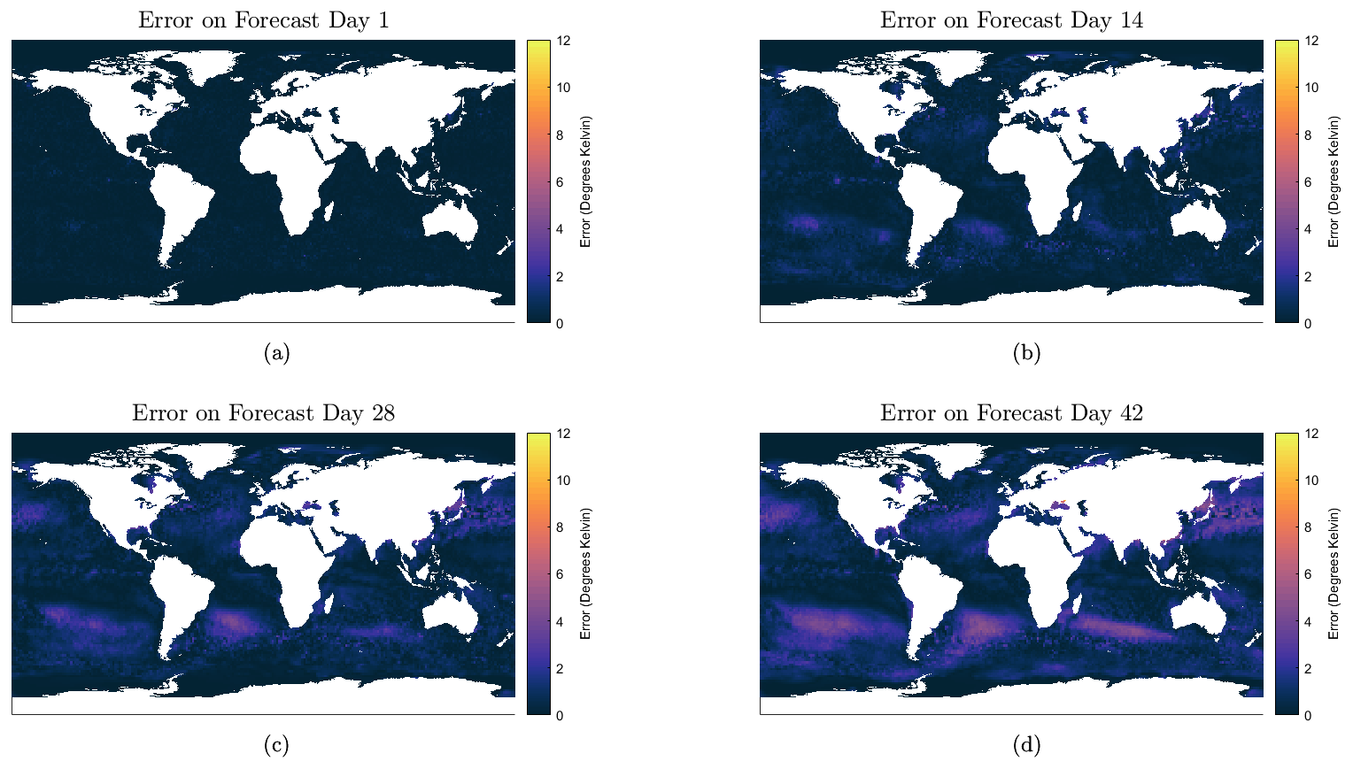
Figure 8The evolution of the error across the globe for the 6-week forecast. The error at each location is simply the difference between the average forecasted value and the actual value.

Figure 9The evolution of the error for the 6-week forecast. The average model error statistics are plotted each day as well as ±1 standard deviation. The mean absolute error in the forecast over the entire ocean is depicted in panel (a), the root-mean-square error is shown in panel (b) and the maximum error is presented in panel (c).
From Fig. 8, it is observed that the model generally performs the best near the Equator, with some slight difficulty predicting the general warming of the ocean in the Southern Hemisphere and cooling in the Northern Hemisphere during this time frame. The average MAE and RMSE rise to 0.32 and 0.45 K, respectively, on the seventh day of forecasting, subsequently increasing to respective values of 0.73 and 0.99 K by the end of 4 weeks. For context, for a prediction horizon of 1 week, Xiao et al. (2019b) reported a RMSE of 0.85 K and Shi et al. (2022) reported a RMSE of 0.687 K for their respective models mentioned previously. Meanwhile for a prediction horizon of 4 weeks, Yang et al. (2018) reported a RMSE of 0.726 K for their CFCC-LSTM (fully connected long short-term memory and convolutional network) model forecasting over the Bohai Sea and a RMSE of 1.070 K for the Chinese coastal waters. Similar to the daily forecasts, it is also apparent that there is little deviation in the RMSE and MAE across the 15 models, once again indicating that the models typically perform similarly regardless of the random weights that they are constructed from.
With the use of coupled reservoir computers, specifically a collection of patches that represent local regions and are designed to accommodate land–water interface variations, we were able to model for excellent forecasting of the spatiotemporally complex dynamics of the global SST over several weeks. The relative simplicity of the network architecture and the minimal training time is striking relative to other machine learning concepts. Even though our model is intended to describe the dynamics of the entire ocean, it is still able to predict the SST at specific locations. In the future, it is of interest to explore the use of next-generation reservoir computers (NG-RCs) in the task of predicting SST, as NG-RCs provide the added benefit of less metaparameters to tune compared with a traditional RC (Jaeger and Haas, 2004; Bollt, 2021; Gauthier et al., 2021). It is also of interest to input other variables into the reservoir besides the SST, such as the surrounding air temperature (Jahanbakht et al., 2021), in order to observe if the results can be further improved.
The code is available online at https://github.com/BenWalleshauser/Predicting-SST-w-.-Coupled-RCs (last access: 29 June 2022) and https://doi.org/10.5281/zenodo.6647777 (Walleshauser, 2022).
EB conceived the idea for the study, and BW was responsible for the creation of the model. BW and EB both contributed to the analyses and the creation of the paper.
The contact author has declared that none of the authors has any competing interests.
Publisher’s note: Copernicus Publications remains neutral with regard to jurisdictional claims in published maps and institutional affiliations.
Erik Bollt received funding from the Army Research Office (ARO), the Defense Advanced Research Projects Agency (DARPA), the National Science Foundation (NSF) and National Institutes of Health (NIH) CRNS program, and the Office of Naval Research (ONR) during the period of this work.
This research has been supported by the Army Research Office (grant no. N68164-EG).
This paper was edited by Reik Donner and reviewed by two anonymous referees.
Bollt, E.: On explaining the surprising success of reservoir computing forecaster of chaos? The universal machine learning dynamical system with contrast to VAR and DMD, Chaos, 31, 013108, https://doi.org/10.1063/5.0024890, 2021. a, b
Case, J. L., Santos, P., Lazarus, S. M., Splitt, M. E., Haines, S. L., Dembek, S. R., and Lapenta, W. M.: A Multi-Season Study of the Effects of MODIS Sea-Surface Temperatures on Operational WRF Forecasts at NWS Miami, FL, New Orleans, LA, https://ntrs.nasa.gov/citations/20080014843 (last access: 29 June 2022), 2008. a
Collins, D. C., Reason, C. J. C., and Tangang, F.: Predictability of Indian Ocean sea surface temperature using canonical correlation analysis, Clim. Dynam., 22, 481–497, https://doi.org/10.1007/s00382-004-0390-4, 2004. a
Dado, J. M. B. and Takahashi, H. G.: Potential impact of sea surface temperature on rainfall over the western Philippines, Prog. Earth Planet. Sci., 4, 23, https://doi.org/10.1186/s40645-017-0137-6, 2017. a
Gauthier, D. J., Bollt, E., Griffith, A., and Barbosa, W. A. S.: Next generation reservoir computing, Nat. Commun., 12, 5564, https://doi.org/10.1038/s41467-021-25801-2, 2021. a
Ghosh, S., Senapati, A., Mishra, A., Chattopadhyay, J., Dana, S., Hens, C., and Ghosh, D.: Reservoir computing on epidemic spreading: A case study on COVID-19 cases, Phys. Rev. E, 104, 014308, https://doi.org/10.1103/PhysRevE.104.014308, 2021. a
Gomez, A. M., McDonald, K. C., Shein, K., DeVries, S., Armstrong, R. A., Hernandez, W. J., and Carlo, M.: Comparison of Satellite-Based Sea Surface Temperature to In Situ Observations Surrounding Coral Reefs in La Parguera, Puerto Rico, J. Mar. Eng., 8, 453, https://doi.org/10.3390/jmse8060453, 2020. a
Hadaeghi, F., Diercks, B.-P., Schetelig, D., Damicelli, F., Wolf, I. M. A., and Werner, R.: Spatio-temporal feature learning with reservoir computing for T-cell segmentation in live-cell CA2+ fluorescence microscopy, Sci. Rep., 11, 8233, https://doi.org/10.1038/s41598-021-87607-y, 2021. a
Jaeger, H. and Haas, H.: Harnessing Nonlinearity: Predicting Chaotic Systems and Saving Energy in Wireless Communication, Science, 304, 78–80, https://doi.org/10.1126/science.1091277, 2004. a, b
Jahanbakht, M., Xiang, W., and Azghadi, M. R.: Sea Surface Temperature Forecasting With Ensemble of Stacked Deep Neural Networks, IEEE Geosci. Remote S., 19, 1–5, https://doi.org/10.1109/LGRS.2021.3098425, 2021. a
Jiang, J. and Lai, Y.-C.: Model-free prediction of spatiotemporal dynamical systems with recurrent neural networks: Role of network spectral radius, Phys. Rev. Res., 1, 033056, https://doi.org/10.1103/PhysRevResearch.1.033056, 2019. a
Johnson, S. D., Battisti, D. S., and Sarachik, E. S.: Empirically Derived Markov Models and Prediction of Tropical Pacific Sea Surface Temperature Anomalies, J. Climate, 13, 3–17, https://doi.org/10.1175/1520-0442(2000)013<0003:EDMMAP>2.0.CO;2, 2000. a
Kim, M., Yang, H., and Kim, J.: Sea Surface Temperature and High Water Temperature Occurrence Prediction Using a Long Short-Term Memory Model, Remote Sens., 12, 3654, https://doi.org/10.3390/rs12213654, 2020. a
Krishnamurti, T. N., Chakraborty, A., Krishnamurti, R., Dewar, W. K., and Clayson, C. A.: Seasonal Prediction of Sea Surface Temperature Anomalies Using a Suite of 13 Coupled Atmosphere–Ocean Models, J. Climate, 19, 6069–6088, https://doi.org/10.1175/JCLI3938.1, 2006. a
Kug, J.-S., Kang, I.-S., Lee, J.-Y., and Jhun, J.-G.: A statistical approach to Indian Ocean sea surface temperature prediction using a dynamical ENSO prediction, Geophys. Res. Lett., 31, 09212, https://doi.org/10.1029/2003GL019209, 2004. a
Lins, I. D., Araujo, M., Moura, M. d. C., Silva, M. A., and Droguett, E. L.: Prediction of sea surface temperature in the tropical Atlantic by support vector machines, Comput. Stat. Data An., 61, 187–198, https://doi.org/10.1016/j.csda.2012.12.003, 2013. a
Novi, L., Bracco, A., and Falasca, F.: Uncovering marine connectivity through sea surface temperature, Sci. Rep., 11, 8839, https://doi.org/10.1038/s41598-021-87711-z, 2021. a
Pandey, S. and Schumacher, J.: Reservoir computing model of two-dimensional turbulent convection, Phys. Rev. Fluids, 5, 113506, https://doi.org/10.1103/PhysRevFluids.5.113506, 2020. a
Pastor, F.: Sea Surface Temperature: From Observation to Applications, J. Mar. Sci. Eng., 9, 1284, https://doi.org/10.3390/jmse9111284, 2021. a
Pathak, J., Hunt, B., Girvan, M., Lu, Z., and Ott, E.: Model-Free Prediction of Large Spatiotemporally Chaotic Systems from Data: A Reservoir Computing Approach, Phys. Rev. Lett., 120, 024102, https://doi.org/10.1103/PhysRevLett.120.024102, 2018. a
PO.DAAC: JPL MUR MEaSUREs Project – GHRSST Level 4 MUR 0.25 deg Global Foundation Sea Surface Temperature Analysis (v.4.2), PO.DAAC [data set], CA, USA, https://doi.org/10.5067/GHM25-4FJ42, 2019. a, b
Patil, K., Deo, M. C., and Ravichandran, M.: Prediction of Sea Surface Temperature by Combining Numerical and Neural Techniques, J. Atmos. Ocean. Tech., 33, 1715–1726, https://doi.org/10.1175/JTECH-D-15-0213.1, 2016. a
Shi, J., Yu, J., Yang, J., Xu, L., and Xu, H.: Time Series Surface Temperature Prediction Based on Cyclic Evolutionary Network Model for Complex Sea Area, Future Internet, 14, 96, https://doi.org/10.3390/fi14030096, 2022. a, b
Stockdale, T. N., Balmaseda, M. A., and Vidard, A.: Tropical Atlantic SST Prediction with Coupled Ocean–Atmosphere GCMs, J. Climate, 19, 6047–6061, https://doi.org/10.1175/JCLI3947.1, 2006. a
Vlachas, P. R., Pathak, J., Hunt, B. R., Sapsis, T. P., Girvan, M., Ott, E., and Koumoutsakos, P.: Backpropagation algorithms and Reservoir Computing in Recurrent Neural Networks for the forecasting of complex spatiotemporal dynamics, Neural Networks, 126, 191–217, https://doi.org/10.1016/j.neunet.2020.02.016, 2020. a
Walleshauser, B.: BenWalleshauser/Predicting-SST-w-.-Coupled-RCs: Predicting SST w Coupled RCs (SST_Archive), Zenodo [code], https://doi.org/10.5281/zenodo.6647777, 2022. a
Xiao, C., Chen, N., Hu, C., Wang, K., Gong, J., and Chen, Z.: Short and mid-term sea surface temperature prediction using time-series satellite data and LSTM-AdaBoost combination approach, Remote Sens. Environ., 233, 111358, https://doi.org/10.1016/j.rse.2019.111358, 2019a. a
Xiao, C., Chen, N., Hu, C., Wang, K., Xu, Z., Cai, Y., Xu, L., Chen, Z., and Gong, J.: A spatiotemporal deep learning model for sea surface temperature field prediction using time-series satellite data, Environ. Modell. Softw., 120, 104502, https://doi.org/10.1016/j.envsoft.2019.104502, 2019b. a, b
Xue, Y. and Leetmaa, A.: Forecasts of tropical Pacific SST and sea level using a Markov model, Geophys. Res. Lett., 27, 2701–2704, https://doi.org/10.1029/1999GL011107, 2000. a
Yang, Y., Dong, J., Sun, X., Lima, E., Mu, Q., and Wang, X.: A CFCC-LSTM Model for Sea Surface Temperature Prediction, IEEE Geosci. Remote S., 15, 207–211, https://doi.org/10.1109/LGRS.2017.2780843, 2018. a
Zhang, Q., Wang, H., Dong, J., Zhong, G., and Sun, X.: Prediction of Sea Surface Temperature Using Long Short-Term Memory, IEEE Geosic. S., 14, 1745–1749, 2017. a
Zhang, X., Li, Y., Frery, A., and Ren, P.: Sea Surface Temperature Prediction With Memory Graph Convolutional Networks, IEEE Geosci. Remote S., 19, 8017105, https://doi.org/10.25455/wgtn.15111642.v1, 2021. a
Due to varying values of dx owing to points on land, we cannot share a single input matrix Win between all RCs.