Climate bifurcations in a Schwarzschild equation model of the Arctic atmosphere

A column model of the Arctic atmosphere is developed including the nonlinear positive feedback responses of surface albedo and water vapour to temperature. The atmosphere is treated as a grey gas and the flux of longwave radiation is governed by the two-stream Schwarzschild equations. Water vapour concentration is determined by the Clausius–Clapeyron equation. Representative concentration pathways (RCPs) are used to model carbon dioxide concentrations into the future. The resulting 9D two-point boundary value problem is solved under various RCPs and the solutions analysed. The model predicts that under the highest carbon pathway, the Arctic climate will undergo an irreversible bifurcation to a warm steady state, which would correspond to annually ice-free conditions. Under the lowest carbon pathway, corresponding to very aggressive carbon emission reductions, the model exhibits only a mild increase in Arctic temperatures. Under the two intermediate carbon pathways, temperatures increase more substantially, and the system enters a region of bistability where external perturbations could possibly cause an irreversible switch to a warm, ice-free state.

1 Introduction

Climate change is causing rapid temperature increases in the polar regions. A fundamental question is whether these temperature increases are reversible. If humanity fails to prevent a substantial warming of the planet in the next few decades, which is appearing to be more and more likely, will it be possible in the future to reverse our effects on climate enough to restore lower temperatures, or will we have passed a tipping point beyond which return to the present state is impossible? We address this question in particular for the Arctic, where the observed climate change is the most dramatic.

The Earth's climate is an extremely complex system. Modelling efforts range from simple models attempting to isolate the most pertinent features to very complicated numerical models trying to capture as many details as possible. The model presented here is close to the simple end of this spectrum, although not as simple as some, in that it is a 9D nonlinear two-point boundary value problem. The advantage of relatively simple models is that they allow more direct analysis of cause and effect, which is often obscured in highly complicated models.

The term “tipping point” is used by different researchers in various ways; see Russill (2015) and Lenton et al. (2008) for some definitions and discussion of the term. In all cases, however, tipping points are associated with large qualitative changes in a system due to relatively small changes in the parameters or “forcings” that drive the system. In the present paper, tipping points arise as a result of saddle-node and cusp bifurcations in the mathematical model. The mathematical theory of bifurcations is well-developed (Kuznetsov, 2004) and employed here. Figure 1 illustrates the typical behaviour associated with these bifurcations. In Fig. 1a there are two saddle-node bifurcations resulting in a parameter interval of bistability; that is, two stable states coexist for an interval of μ values. If the system is on the lower branch of stable states, then, as μ increases through a critical value μ_crit, there is an abrupt jump to the upper branch of stable states. In contrast, as μ decreases, the jump back to the lower state does not occur until a much smaller critical value of μ. This phenomenon is called hysteresis. If present in the Earth's climate system, it implies that once the upward jump occurs, it may be very difficult to achieve the reverse jump back to the original climate state. Figure 1b illustrates the situation of a cusp bifurcation, where the two saddle-node bifurcations in Fig. 1a have coalesced, for example, as another parameter of the system is varied. In this situation a small change in μ will also cause a large change in the system F, although it will be smooth and reversible. In Fig. 1c, even though the saddle-node bifurcations may be outside the parameter interval of interest, abrupt large transitions in the system can result from a small noise- or perturbation-induced change to the system even when the parameter value remains constant. It is the presence of saddle-node bifurcations in a mathematical model, even if not occurring precisely at the system's current parameter value, that is the root cause of all of the behaviours shown in Fig. 1.

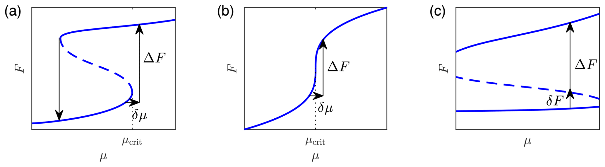
Figure 1 (a) Hysteresis arising from two saddle-node bifurcations. (b) A cusp bifurcation. (c) A bistable system. Solid curves indicate stable states, and dashed curves are unstable states. In panels (a) and (b) a small change δμ in the control parameter near the bifurcation value μ_crit causes a large change ΔF in the system. In panel (a) the return bifurcation happens at a different value of μ. In panel (c) a small perturbation δF in the system causes a large change ΔF.

For a tipping point to be present, the underlying mathematical model will be characterized by nonlinearity, generally in the form of a positive feedback that accelerates change once change has begun. For the Arctic, one of the primary positive feedbacks is the surface albedo. When the Arctic Ocean is frozen, the surface reflects a significant portion of the insolation back into space, but open water absorbs much more heat from the Sun. Timing of the melt in the spring has significant impact (Zheng et al., 2021). An earlier melt means considerably more heat is absorbed by open water, raising the water temperature and delaying freeze-up in the autumn. The freeze-up date for the Beaufort, Chukchi, Laptev, and Kara seas, for example, has been getting later by 6–11 d per decade since 1979 (Stroeve et al., 2014). September sea ice extent has been decreasing at an accelerating rate. The linear trend from 1979 to 2001 is −7 % per decade, but including data up to 2013, the linear trend is −14 % per decade (Stroeve et al., 2014). Thus the observational evidence indicates that the processes behind this phenomenon are not linear at all but nonlinear.

Past studies on general circulation models (GCMs) have given mixed results regarding the presence of multiple stable states for ice conditions in the Arctic. Some indicate that there appears to be a continuous transition from perennial ice cover to annually ice-free that is reversible (Schröder and Connolley, 2007; Tietsche et al., 2011; Armour et al., 2011). Other studies have shown evidence for nonlinear behaviour in sea ice loss, especially in the transition from seasonally ice-free to annually ice-free (Winton, 2006, 2008; Ridley et al., 2008). On the other hand, smaller conceptual models generally show bistability and abrupt transitions in sea ice cover (Thorndike, 1992; Müller-Stoffels and Wackerbauer, 2011; Eisenman and Wettlaufer, 2009; Björk and Söderkvist, 2002; Abbot et al., 2011; Merryfield et al., 2008; Flato and Brown, 1996). The most common result from all these models seems to be that sea ice will likely transition from perennial to seasonally ice-free in a continuous, reversible manner, but significant warming beyond that point will likely cause an abrupt change to annually ice-free (Bathiany et al., 2016). See the introduction in Eisenman (2012). The model we present here is an annually averaged model with no seasonal component. It is not a model of sea ice in particular but rather a column model of the atmosphere that incorporates a nonlinear albedo response to surface temperature. Bistability in our model with both warm and cold solutions corresponds to annually averaged ice-covered or ice-free situations.

The Arctic climate model presented here is motivated by three observations. First is the observation that the climate changes taking place on the Earth today are most dramatic in the high Arctic. Therefore, it is prudent to put a special focus on understanding Arctic climate change. Second, irreversible change is inevitably the result of nonlinear geophysical processes. So, while this model is kept very simple, it does include significant nonlinear phenomena that can lead to tipping points. Third, the 3D spherical shell of the atmosphere of the Earth is rotationally symmetric about the polar axis if annually and zonally averaged. Due to the rotation of the Earth, Hadley, Ferrel and polar cells form in the global circulation. If perfect rotational symmetry is assumed, the polar axis becomes flow-invariant, and this remains approximately true for the real Earth. Thus, a 1D model restricted to the polar axis can be expected to give useful information about climate in a neighbourhood of the pole. The study of a rotationally symmetric spherical shell model by Lewis and Langford (2008) gives support to this hypothesis. A vertical column of atmosphere at other points on Earth would have a horizontal component of velocity, invalidating the type of analysis used here. Globally averaged climate models do reduce to one (vertical) dimension, but they give little information specific to the Arctic.

The present model builds on the simple energy balance slab model of Dortmans et al. (2019), which was applied to paleoclimate transitions, and the model of Kypke et al. (2020), which was applied to anthropogenic climate change. The primary improvement of the present model is a more physically accurate description of the atmosphere. Instead of using a slab to represent a uniform atmosphere with absorption properties similar to the real atmosphere, here we use the Schwarzschild two-stream equations to model absorption in the atmosphere explicitly as a function of altitude (Pierrehumbert, 2010, p. 191).

A bifurcation analysis is performed on the model, tracking the steady-state solutions as carbon dioxide levels increase. The question of reversibility is a question of whether the current cold state simply warms but persists. The disappearance of this cold state through a saddle-node bifurcation would result in an abrupt change in climate that may be practically irreversible. The simpler model of Kypke et al. (2020) showed this behaviour under certain CO₂ representative concentration pathway scenarios. We seek here to determine whether the present, more accurate model also displays this behaviour.

Section 2 and Appendix A provide a detailed derivation of the model. The model parameter values and calibration of some of them to empirical data are presented in Appendix B. Although much of the detail is relegated to the Appendices, the authors feel this detail constitutes an essential part of the contribution of the paper, providing clarity, justification of choices, and the information necessary for replication. Hence we consider them essential reading. Section 3 presents the results, and the conclusions are in Sect. 4.

2 Model

The model is developed from first principles and has the following features.

• The atmosphere is a 1D column at the North Pole with physical properties that vary with altitude, from the surface to the tropopause.

• The incoming solar radiation is annually averaged and undergoes reflection and absorption in the atmosphere as well as at the Earth's surface.

• The surface albedo is a nonlinear function of the surface temperature.

• A well-mixed surface boundary layer is included.

• The Earth emits longwave radiation as a black body.

• The atmosphere is considered to be a grey gas.

• The Schwarzschild two-stream equations govern the absorption and emission of both upward- and downward-directed longwave radiation in the atmosphere.

• The atmospheric absorption of longwave radiation is due to three factors: water vapour, CO₂ concentration, and clouds.

• Water vapour concentration is governed by the nonlinear Clausius–Clapeyron equation.

• Transfer of latent and sensible heat from the surface to the atmosphere is modelled.

• Both ocean and atmospheric meridional heat transports to the Arctic are dictated by empirical values.

• In the Arctic, there is a slow downward movement of air in the column corresponding to the polar circulation cell near the pole (Lewis and Langford, 2008; Langford and Lewis, 2009; Lutgens and Tarbuck, 2019). This is achieved via mass transport of air into the column in its upper portion and out of the column near the bottom.

• The radiation absorption coefficients are calibrated by fitting the model to global average data.

• The functional forms of the mass transport and atmospheric heat transport are used to calibrate the model to an empirical Arctic temperature profile.

The annually and zonally averaged Earth atmosphere is rotationally symmetric around the polar axis, which is invariant under the flow. Therefore, if one considers a column of the atmosphere near the North Pole, it is reasonably approximated by a 1D model with altitude-varying quantities. This approximation becomes exact in the limit as the diameter of the column shrinks to zero. Alternatively, one can view the model as a meridional and zonal average over a cylinder centred at the North Pole. Further, although the Arctic Ocean is not zonally symmetric, in the above view, the contribution of ocean heat transport can be reasonably captured as a scalar quantity. Thus our model is more precisely a model of the North Pole rather than the Arctic. Nonetheless, we do use some empirical data for the region north of 70^∘ to calibrate the model for two reasons: (1) data further north are not readily available, and (2) the data we use are not likely to alter too much if they were measured closer to the pole. The values for atmospheric heat transport and ocean heat transport are two that may change significantly as one moves north from 70^∘, and we therefore analyse the behaviour of the model over a wide range for these parameter values.

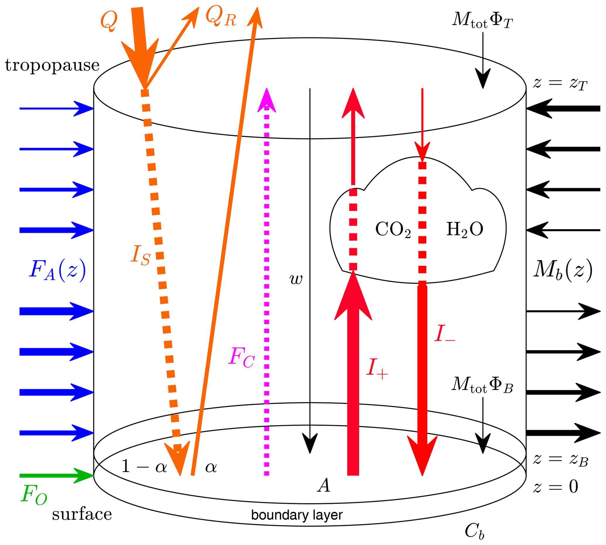
The model domain is a vertical cylinder of cross-sectional area A (m²) and circumference C_b (m). The atmosphere is assumed to be uniform in the cross-sectional direction, so that the model's dependent variables can be interpreted as cross-sectional averages that vary with the 1D vertical coordinate $z\in [\mathrm{0},z_{\mathrm{T}}]$, where z_T (m) is the height of the tropopause. This domain is divided into a surface boundary layer with height z_B (m), z_B≪z_T, and the troposphere proper, $z\in [z_{\mathrm{B}},z_{\mathrm{T}}]$. The model consists of a set of initial value problems (IVPs), with an independent spatial variable z on [0,z_B], which can be solved analytically, and a two-point boundary value problem (BVP) on [z_B,z_T] that depends on the solutions to the IVPs. The model has equations governing the vertical wind speed, w (m s⁻¹), the air density, ρ (kg m⁻³), the upward and downward longwave radiation, I₊ and I₋ (W m⁻²), the downward shortwave radiation, I_S (W m⁻²), the latent and sensible heat transport, F_C (W m⁻²), and the temperature T (K). Any reflection of shortwave radiation from either the surface or the atmosphere is ignored and is simply considered to have left the system. The model is depicted in Fig. 2 and is derived and explained in detail in the following subsections. Many of the details of the model, including its nondimensionalization, the vanishing conduction limit, and modelling choices used for various functional forms, are in Appendix A. Calibration of the model parameters to empirical data is described in detail in Appendix B, and the reader is referred to Tables B1 and B2 of that appendix for the values of the parameters.

Figure 2 Schematic illustration of the model. Symbols as described in the text.

2.1 Mass, momentum, and energy balance

The model equations in the troposphere are developed from the fundamental transport theorem in one spatial dimension:

$$\begin{array}{}\text{(1)}& {\partial }_{t}f+{\partial }_z\mathit{\chi }=S,\end{array}$$

where f is the density of some “property”, χ is the flux of that property, and S is a source/sink term. The time-derivative term will be taken as zero since only the steady-state solution is considered. The properties subject to this equation are mass, momentum, and energy. To model the Arctic, the cylinder is centred at the North Pole, and, since the atmospheric polar cell has slow downward movement near the pole, it is assumed that w<0.

2.1.1 Mass

If the property f in Eq. (1) is the mass density, ρ (kg m⁻³), then the flux is χ=ρw. There is mass flux across the vertical boundary of the cylinder, M_b(z) ($\mathrm{kg}{\mathrm{m}}^{-\mathrm{2}}{\mathrm{s}}^{-\mathrm{1}}$), which is assumed to be immediately spread out evenly across the layer, and hence the mass flux across the vertical boundary in the model is really a mass source term in the interior giving

$$\begin{array}{rl}S& ={\displaystyle \frac{\text{mass entering into cylinder layer of width}\mathrm{\Delta }z}{\text{volume of layer}}}\\ & ={\displaystyle \frac{M_{\mathrm{b}}\left(z\right)C_{\mathrm{b}}\mathrm{\Delta }z}{A\mathrm{\Delta }z}}={\displaystyle \frac{C_{\mathrm{b}}}{A}}{M}_{\mathrm{b}}\left(z\right).\end{array}$$

Thus, at steady state the mass balance equation is

$${\displaystyle \frac{\mathrm{d}\left(\mathit{\rho }w\right)}{\mathrm{d}z}}={\displaystyle \frac{C_{\mathrm{b}}}{A}}{M}_{\mathrm{b}}\left(z\right).$$

The mass flux through the vertical boundary into the column is written as

$$M_{\mathrm{b}}\left(z\right)={\displaystyle \frac{A}{C_{\mathrm{b}}(z_{\mathrm{T}}-z_{\mathrm{B}})}}{M}_{\mathrm{tot}}\mathit{\varphi }\left({\displaystyle \frac{z-z_{\mathrm{B}}}{z_{\mathrm{T}}-z_{\mathrm{B}}}}\right),$$

where M_tot ($\mathrm{kg}{\mathrm{m}}^{-\mathrm{2}}{\mathrm{s}}^{-\mathrm{1}}$) is a nonnegative constant and $\mathit{\varphi }\left(x\right):[\mathrm{0},\mathrm{1}]\mapsto \mathbb{R}$ is a dimensionless function that represents the portion of inward mass flux across the vertical boundary of the column at the given altitude. Positive ϕ indicates inward flow. The ratio of the cross-sectional area of the column to the area of its side, $A/\left(C_{\mathrm{b}}\right(z_{\mathrm{T}}-z_{\mathrm{B}}\left)\right)$, in the definition of M_b(z) is included as a useful simplifying convenience. The (positive inward) mass fluxes across the bottom and top boundaries of the column are given by M_totΦ_B and M_totΦ_T, respectively, where Φ_B and Φ_T are dimensionless constants in the interval $[-\mathrm{1},\mathrm{1}]$. These quantities must satisfy

$$\begin{array}{ll}{\displaystyle }& {\displaystyle }\underset{\mathrm{0}}{\overset{\mathrm{1}}{\int }}\mathit{\varphi }\left(x\right)\mathrm{d}x+{\mathrm{\Phi }}_{\mathrm{B}}+{\mathrm{\Phi }}_{\mathrm{T}}=\mathrm{0}\mathrm{\text{and}}\\ \text{(2)}& {\displaystyle }& {\displaystyle }\underset{\mathrm{0}}{\overset{\mathrm{1}}{\int }}max\left(\mathit{\varphi }\right(x),\mathrm{0})\mathrm{d}x+max({\mathrm{\Phi }}_{\mathrm{B}},\mathrm{0})+max({\mathrm{\Phi }}_{\mathrm{T}},\mathrm{0})=\mathrm{1}.\end{array}$$

The first of these conditions dictates that there is no net mass entering the system, and the second is a normalization condition so that M_tot represents both the total mass entering the column per unit cross-sectional area and the magnitude of the total mass leaving the column per unit cross-sectional area. In order to obtain downward vertical flow throughout the cylinder, it shall be assumed that Φ_B<0, Φ_T>0, ϕ≤0 in the lower part of the cylinder and ϕ≥0 in the upper part. With these definitions, the mass balance equation becomes

$$\begin{array}{}\text{(3)}& {\displaystyle \frac{\mathrm{d}\left(\mathit{\rho }w\right)}{\mathrm{d}z}}={\displaystyle \frac{M_{\mathrm{tot}}}{z_{\mathrm{T}}-z_{\mathrm{B}}}}\mathit{\varphi }\left({\displaystyle \frac{z-z_{\mathrm{B}}}{z_{\mathrm{T}}-z_{\mathrm{B}}}}\right).\end{array}$$

2.1.2 Momentum

Now take the property f in Eq. (1) to be the momentum density, ρw. The vertical flux is χ=ρw², and the source term S has two components, one due to contact forces (stress) (van Groesen and Molenaar, 2017, p. 56) and one due to internal body forces (gravity):

$$S=-{\displaystyle \frac{\mathrm{d}P}{\mathrm{d}z}}-\mathit{\rho }g,$$

where P (N m⁻²) is the pressure and g (m s⁻²) is the gravitational acceleration. It is assumed that mass entering the cylinder from the vertical boundary has no vertical momentum. Thus the momentum balance equation at steady state is

$$\begin{array}{}\text{(4)}& {\displaystyle \frac{\mathrm{d}\left(\mathit{\rho }{w}^{\mathrm{2}}\right)}{\mathrm{d}z}}=-{\displaystyle \frac{\mathrm{d}P}{\mathrm{d}z}}-\mathit{\rho }g.\end{array}$$

(In the case of no flow (w=0), the above would read $\mathrm{d}P/\mathrm{d}z=-\mathit{\rho }g$, which is the hydrostatic equation.)

2.1.3 Energy

Finally, consider the case where the property in Eq. (1) is the total energy density given by

$$e={\displaystyle \frac{\mathrm{1}}{\mathrm{2}}}\mathit{\rho }{w}^{\mathrm{2}}+\mathit{\rho }gz+c_v\mathit{\rho }T,$$

which corresponds to the sum of kinetic energy, gravitational potential energy, and internal heat energy densities. Here, c_v ($\mathrm{J}{\mathrm{kg}}^{-\mathrm{1}}{\mathrm{K}}^{-\mathrm{1}}$) is the specific heat capacity of the air. The flux has two components, one due to advection and one due to conduction:

$$\mathit{\chi }=ew-k{\displaystyle \frac{\mathrm{d}T}{\mathrm{d}z}},$$

where k ($\mathrm{W}{\mathrm{m}}^{-\mathrm{1}}{\mathrm{K}}^{-\mathrm{1}}$) is the thermal conductivity. The source/sink S has eight terms, one due to work done by contact forces, two due to mass entering or leaving across the vertical boundary (one of these accounts for gravitational potential energy and the other internal heat energy; there is no addition to kinetic energy since the mass appearing has no velocity), three due to radiation (shortwave downward and longwave upward and downward), one due to latent and sensible heat transport, and one due to atmospheric heat transport. It is important to distinguish the difference between the mass transport across the boundary and the atmospheric heat transport. It is assumed that the mass moving across the vertical boundary is at the same temperature as the mass inside at each altitude. Since mass transfer across the vertical boundary is inward in the upper portion, where the temperature is cooler, and outward in the bottom portion, mass transport results in a net transport of heat out through the vertical boundary, but this will be small since the mass flux, M_b(z), is small. The reason M_b(z) is small is that it generates the average slow movement of air downward near the North Pole (about 1 mm s⁻¹), due to the circulation of the polar cell. This slow averaged circulation of air does not account for the atmospheric heat transport. The main transport of heat in the atmosphere is via turbulent mixing captured in our model by a source term, F_A(z) (W m⁻³), whose functional form is discussed in Sect. A3. Thus, S is given by

$$\begin{array}{rl}S=& -{\displaystyle \frac{\mathrm{d}\left(Pw\right)}{\mathrm{d}z}}+{\displaystyle \frac{M_{\mathrm{tot}}}{z_{\mathrm{T}}-z_{\mathrm{B}}}}\mathit{\varphi }\left({\displaystyle \frac{z-z_{\mathrm{B}}}{z_{\mathrm{T}}-z_{\mathrm{B}}}}\right)gz\\ & +{\displaystyle \frac{M_{\mathrm{tot}}}{z_{\mathrm{T}}-z_{\mathrm{B}}}}\mathit{\varphi }\left({\displaystyle \frac{z-z_{\mathrm{B}}}{z_{\mathrm{T}}-z_{\mathrm{B}}}}\right)c_{v}T\\ & -{\displaystyle \frac{\mathrm{d}{I}_{+}}{\mathrm{d}z}}+{\displaystyle \frac{\mathrm{d}{I}_{-}}{\mathrm{d}z}}+{\displaystyle \frac{\mathrm{d}{I}_{\mathrm{S}}}{\mathrm{d}z}}-{\displaystyle \frac{\mathrm{d}{F}_{\mathrm{C}}}{\mathrm{d}z}}+F_{\mathrm{A}}\left(z\right).\end{array}$$

The governing equations for the longwave radiation intensities are the two-stream Schwarzschild equations and for the shortwave radiation a standard absorption equation:

$$\begin{array}{}\text{(5)}& {\displaystyle \frac{\mathrm{d}{I}_{+}}{\mathrm{d}z}}& {\displaystyle }=-\mathit{\kappa }(I_{+}-\mathit{\sigma }{T}^{\mathrm{4}}),\text{(6)}& {\displaystyle \frac{\mathrm{d}{I}_{-}}{\mathrm{d}z}}& {\displaystyle }=\mathit{\kappa }(I_{-}-\mathit{\sigma }{T}^{\mathrm{4}}),\text{(7)}& {\displaystyle \frac{\mathrm{d}{I}_{\mathrm{S}}}{\mathrm{d}z}}& {\displaystyle }=k_{\mathrm{S}}\mathit{\rho }{I}_{\mathrm{S}},\end{array}$$

where k_S (m² kg⁻¹) is the shortwave absorption coefficient, σ ($\mathrm{W}{\mathrm{m}}^{-\mathrm{2}}{\mathrm{K}}^{-\mathrm{4}}$) is the Stefan–Boltzmann constant, and κ (m⁻¹) is the longwave absorption coefficient with terms corresponding to absorption by clouds, carbon dioxide, and water vapour:

$$\begin{array}{ll}{\displaystyle }\mathit{\kappa }(\mathit{\rho },T)=& {\displaystyle }{k}_{\mathrm{Cl}}+k_{\mathrm{C}}{\displaystyle \frac{M_{{\mathrm{CO}}_{\mathrm{2}}}}{M_{\mathrm{A}}}}\left({\displaystyle \frac{\mathit{\mu }}{{\mathrm{10}}^{\mathrm{6}}}}\right)\mathit{\rho }\\ \text{(8)}& {\displaystyle }& {\displaystyle }+k_{\mathrm{W}}\mathit{\delta }\left({\displaystyle \frac{z-z_{\mathrm{B}}}{z_{\mathrm{T}}-z_{\mathrm{B}}}}\right)P^{\mathrm{sat}}\left(T\right).\end{array}$$

Here, k_Cl (m⁻¹), k_C (m² kg⁻¹), and k_W (s² kg⁻¹) are absorption coefficients that will be calibrated, μ (ppm) is the CO₂ concentration expressed as the ratio of moles of CO₂ to moles of dry air, $M_{{\mathrm{CO}}_{\mathrm{2}}}$ and M_A (kg mol⁻¹) are the molar masses of CO₂ and dry air, respectively, $\mathit{\delta }\left(\right(z-z_{\mathrm{B}})/(z_{\mathrm{T}}-z_{\mathrm{B}}\left)\right)$ is the relative humidity at altitude z, and P^sat(T) (N m⁻¹) is the saturated water vapour partial pressure at temperature T. The dependence of this last quantity on T is given by the Clausius–Clapeyron equation

$$\begin{array}{}\text{(9)}& P^{\mathrm{sat}}\left(T\right)=P^{\mathrm{sat}}\left(T_{\mathrm{R}}\right)\exp \left({\displaystyle \frac{L_{\mathrm{v}}}{R_{\mathrm{W}}{T}_{\mathrm{R}}}}{\displaystyle \frac{T-T_{\mathrm{R}}}{T}}\right),\end{array}$$

where P^sat(T_R) is the pressure at a reference temperature T_R (which we take to be 273.15 K), L_v (m² s⁻²) is the latent heat of vaporization for water, and $R_{\mathrm{W}}=R/M_{\mathrm{W}}$ ($\mathrm{J}{\mathrm{K}}^{-\mathrm{1}}{\mathrm{kg}}^{-\mathrm{1}}$) is the gas constant for water, R ($\mathrm{J}{\mathrm{K}}^{-\mathrm{1}}{\mathrm{mol}}^{-\mathrm{1}}$) is the universal gas constant, and M_W (kg mol⁻¹) is the molar mass of water. The corresponding density is ${\mathit{\rho }}_{\mathrm{W}}^{\mathrm{sat}}\left(T\right)=P^{\mathrm{sat}}\left(T\right)/\left(R_{\mathrm{W}}T\right)$ by the ideal gas law. The vertical heat transport (latent and sensible heat) is assumed to be governed by a simple exponential decay:

$$\begin{array}{}\text{(10)}& {\displaystyle \frac{\mathrm{d}{F}_{\mathrm{C}}}{\mathrm{d}z}}=-b{F}_{\mathrm{C}},\end{array}$$

where b (m⁻¹) is a suitable decay constant. Substituting these expressions for the total energy density and its flux and sources into Eq. (1) and combining the expressions from Eqs. (5) to (10), the energy balance equation at steady state for $z\in [z_{\mathrm{B}},z_{\mathrm{T}}]$ is given by

$$\begin{array}{}\text{(11)}& \begin{array}{rl}& {\displaystyle \frac{\mathrm{d}}{\mathrm{d}z}}\left({\displaystyle \frac{\mathrm{1}}{\mathrm{2}}}\mathit{\rho }{w}^{\mathrm{3}}+\mathit{\rho }gzw+c_v\mathit{\rho }Tw\right)-k{\displaystyle \frac{{\mathrm{d}}^{\mathrm{2}}T}{\mathrm{d}{z}^{\mathrm{2}}}}=-{\displaystyle \frac{\mathrm{d}\left(Pw\right)}{\mathrm{d}z}}\\ & +{\displaystyle \frac{M_{\mathrm{tot}}}{z_{\mathrm{T}}-z_{\mathrm{B}}}}\mathit{\varphi }\left({\displaystyle \frac{z-z_{\mathrm{B}}}{z_{\mathrm{T}}-z_{\mathrm{B}}}}\right)\left(gz+c_{v}T\right)\\ & +\mathit{\kappa }(\mathit{\rho },T)(I_{+}+I_{-}-\mathrm{2}\mathit{\sigma }{T}^{\mathrm{4}})+k_{\mathrm{S}}\mathit{\rho }{I}_{\mathrm{S}}+b{F}_{\mathrm{C}}+F_{\mathrm{A}}\left(z\right).\end{array}\end{array}$$

The nonlinear effects of both water vapour and carbon dioxide concentration on longwave radiation absorption in the atmosphere are contained within the factor κ(ρ,T), defined by Eq. (8). In earlier work (Dortmans et al., 2019; Kypke et al., 2020), these two effects were studied separately before combining them. It was shown there that, if the atmosphere becomes warmer, then the concentration of water vapour increases due to the Clausius–Clapeyron relation, and this accelerates the greenhouse warming of the atmosphere well beyond that due to carbon dioxide alone. This is an important positive feedback in the model.

In order to complete the system, a constitutive relation between the density ρ and the pressure P is needed, for which we use the ideal gas law,

$$\begin{array}{}\text{(12)}& P=R_{\mathrm{A}}\mathit{\rho }T,\end{array}$$

where $R_{\mathrm{A}}=R/M_{\mathrm{A}}$ ($\mathrm{J}{\mathrm{kg}}^{-\mathrm{1}}{\mathrm{K}}^{-\mathrm{1}}$) is the gas constant for air.

The mass, momentum, and energy balance equations, Eqs. (3), (4), and (11), along with the Schwarzschild equations (Eqs. 5 and 6) and the equations governing shortwave absorption (Eq. 7) and sensible and latent heat transport (Eq. 10) are the differential equations for the BVP for $z\in [z_{\mathrm{B}},z_{\mathrm{T}}]$, with dependent variables w, ρ, I₊, I₋, I_S, F_C, T, and $\mathrm{d}T/\mathrm{d}z$. Equations (8), (9), and (12) define certain quantities in these differential equations in terms of these dependent variables. The forms of the functions F_A(z) and ϕ(z) are prescribed; the process of choosing these functions is described in detail in Appendix A3.2 and A3.3, respectively. Before discussing the boundary conditions for the BVP, it is necessary to consider the surface boundary layer.

2.2 Surface boundary layer

The model includes a boundary layer extending from z=0 to z=z_B. It is assumed that this layer is well-mixed so that temperature T_B=T(z_B), density ρ_B=ρ(z_B), and relative humidity δ_B=δ(z_B) in this layer are constant. The temperature of the surface, T_S, can in general be larger or smaller than T_B.

The primary reason for including a boundary layer is a numerical one. As shown in Appendix A2, the model is numerically stiff due to the thermal conductivity of air being very small. To remove the stiffness, a limit to vanishing conduction is taken, and this results in an algebraic expression for the temperature gradient that includes the vertical wind speed as a factor in the denominator. As the vertical wind speed must be zero at the Earth's surface, there is a singularity in the temperature gradient there. The introduction of the surface boundary layer avoids this singularity.

The total mass crossing from the atmosphere into the boundary layer per unit time is M_totΦ_BA. This quantity is negative, since Φ_B<0, indicating flow out of the atmosphere and into the boundary layer. This mass exits through the vertical boundary of the layer with an assumed constant mass flux K, at each z, and conservation of mass dictates

$$\underset{\mathrm{0}}{\overset{z_{\mathrm{B}}}{\int }}K{C}_{\mathrm{b}}\mathrm{d}z=M_{\mathrm{tot}}{\mathrm{\Phi }}_{\mathrm{B}}A⟹K={\displaystyle \frac{M_{\mathrm{tot}}{\mathrm{\Phi }}_{\mathrm{B}}A}{C_{\mathrm{b}}{z}_{\mathrm{B}}}}.$$

(K<0 indicates the flux is outward.) This exiting mass carries gravitational potential energy. The change in potential energy in a slab of height Δz at height z in the boundary layer is C_bΔzKgz, so that the total change in potential energy over the boundary layer is

$$\begin{array}{}\text{(13)}& {\mathrm{\Delta }}_{\mathrm{PE}}=\underset{\mathrm{0}}{\overset{z_{\mathrm{B}}}{\int }}{C}_{\mathrm{b}}Kgz\mathrm{d}z={\displaystyle \frac{\mathrm{1}}{\mathrm{2}}}{M}_{\mathrm{tot}}{\mathrm{\Phi }}_{\mathrm{B}}Ag{z}_{\mathrm{B}}.\end{array}$$

Consistent with the modelling assumption that mass flux across the vertical boundary conveys no momentum or kinetic energy to the system, the loss of mass out of the vertical boundary of the boundary layer also has no effect on the momentum or kinetic energy. Further, since the temperature in the boundary layer, T_B, is assumed to be equal to the temperature of the atmosphere at z=z_B, it follows that there is also no net energy change in the boundary layer due to advection of internal energy – the internal energy entering via advection at the top of the layer is equal to the internal energy leaving the layer through the vertical boundary.

Consider now the energy balance at the Earth's surface. There is energy transport from the surface to the boundary layer in the form of sensible and latent heat, which is modelled, as per Pierrehumbert (2010, p. 396–398), as

$$\begin{array}{}\text{(14)}& \begin{array}{rl}{F}_{\mathrm{C}\mathrm{0}}({\mathit{\rho }}_{\mathrm{B}},T_{\mathrm{B}},T_{\mathrm{S}})& =F_{\mathrm{C}}\left(\mathrm{0}\right)=F_{\mathrm{sensible}}+F_{\mathrm{latent}}\\ & =c_v{C}_{\mathrm{D}}U{\mathit{\rho }}_{\mathrm{B}}(T_{\mathrm{S}}-T_{\mathrm{B}})\\ & +{\displaystyle \frac{L_{\mathrm{v}}}{R_{\mathrm{W}}{T}_{\mathrm{B}}}}{C}_{\mathrm{D}}U\left(P^{\mathrm{sat}}\right(T_{\mathrm{S}})-\mathit{\delta }(\mathrm{0}\left)P^{\mathrm{sat}}\right(T_{\mathrm{B}}\left)\right),\end{array}\end{array}$$

where C_D is a dimensionless drag coefficient, U (m s⁻¹) is the horizontal wind speed, and P^sat(T) is given by Eq. (9). Along with this there is energy input to the surface from the Sun, I_S(0), some of which is reflected by the surface albedo, longwave radiation both inward, I₋(0), and outward, I₊(0), and ocean heat transport, F_O (W m⁻²). Therefore, the energy balance at the surface is

$$\begin{array}{}\text{(15)}& F_{\mathrm{O}}-I_{+}\left(\mathrm{0}\right)+I_{-}\left(\mathrm{0}\right)+I_{\mathrm{S}}\left(\mathrm{0}\right)(\mathrm{1}-\mathit{\alpha }(T_{\mathrm{S}}\left)\right)-F_{\mathrm{C}}\left(\mathrm{0}\right)=\mathrm{0},\end{array}$$

where

$$\begin{array}{}\text{(16)}& \mathit{\alpha }\left(T_{\mathrm{S}}\right)={\displaystyle \frac{\mathrm{1}}{\mathrm{2}}}\left[({\mathit{\alpha }}_{\mathrm{w}}+{\mathit{\alpha }}_{\mathrm{c}})+({\mathit{\alpha }}_{\mathrm{w}}-{\mathit{\alpha }}_{\mathrm{c}})\tanh \left({\displaystyle \frac{T_{\mathrm{S}}-T_{\mathrm{R}}}{T_{\mathrm{R}}\mathit{\omega }}}\right)\right]\end{array}$$

is the surface albedo, here modelled as a sigmoid function increasing from α_c at cold temperatures to α_w at warm temperatures, with the midway point being at the reference temperature T_R (freezing point) and with a steepness of transition determined by the dimensionless constant ω.

Now consider the energy balance for the combined surface and boundary layer (one could alternatively consider just the boundary layer without the surface, but the chosen formulation results in a slightly smaller equation). Input energy to this combined surface and boundary layer includes ocean heat transport and shortwave and longwave radiation entering at z_B. Output energy includes upward longwave radiation at z_B, the shortwave radiation reflected from the surface, and the latent and sensible heat F_C at z_B. Further, there are kinetic and gravitational potential energy fluxes and heat conduction in/out of the layer through its top at z_B, and there is gravitational potential energy loss through the vertical boundary given by Eq. (13). Therefore, the energy density balance for the combined surface and boundary layer is

$$\begin{array}{}\text{(17)}& \begin{array}{rl}{F}_{\mathrm{O}}& +I_{\mathrm{S}}\left(z_{\mathrm{B}}\right)+I_{-}\left(z_{\mathrm{B}}\right)-I_{+}\left(z_{\mathrm{B}}\right)-I_{\mathrm{S}}\left(\mathrm{0}\right)\mathit{\alpha }\left(T_{\mathrm{S}}\right)\\ & -F_{\mathrm{C}}\left(z_{\mathrm{B}}\right)-{\displaystyle \frac{\mathrm{1}}{\mathrm{2}}}{\mathit{\rho }}_{\mathrm{B}}w(z_{\mathrm{B}}{)}^{\mathrm{3}}-{\mathit{\rho }}_{\mathrm{B}}g{z}_{\mathrm{B}}w(z_{\mathrm{B}})\\ & +k{\displaystyle \frac{\mathrm{d}T}{\mathrm{d}z}}\left(z_{\mathrm{B}}\right)+{\displaystyle \frac{\mathrm{1}}{\mathrm{2}}}g{M}_{\mathrm{tot}}{\mathrm{\Phi }}_{\mathrm{B}}{z}_{\mathrm{B}}=\mathrm{0}.\end{array}\end{array}$$

Since temperature, pressure, and relative humidity are constant in the boundary layer, the radiation equations may be solved analytically inside the layer in order to relate the radiation terms at z=0 to those at z=z_B. The simple ordinary differential equation (ODE) for F_C is also easily solved in the boundary layer. The initial (independent spatial variable z=0) condition for the upward longwave radiation, I₊(0), is that it is equal to the black body radiation of the surface, $\mathit{\sigma }{T}_{\mathrm{S}}^{\mathrm{4}}$. The initial condition for that latent heat, F_C(0), is given by Eq. (14). Initial conditions for I₋ and I_S are not necessary since only a relation between the values of these functions at 0 in terms of their value at z_B is required. The IVPs for I₊ and F_C and the ODEs for I₋ and I_S in the boundary layer are

$$\begin{array}{llll}{\displaystyle \frac{\mathrm{d}{I}_{+}}{\mathrm{d}z}}& {\displaystyle }=-\mathit{\kappa }({\mathit{\rho }}_{\mathrm{B}},T_{\mathrm{B}})(I_{+}-\mathit{\sigma }{T}_{\mathrm{B}}^{\mathrm{4}}),& {\displaystyle }{I}_{+}\left(\mathrm{0}\right)& {\displaystyle }=\mathit{\sigma }{T}_{\mathrm{S}}^{\mathrm{4}},\\ {\displaystyle \frac{\mathrm{d}{F}_{\mathrm{C}}}{\mathrm{d}z}}& {\displaystyle }=-b{F}_{\mathrm{C}},& {\displaystyle }{F}_{\mathrm{C}}\left(\mathrm{0}\right)& {\displaystyle }=F_{\mathrm{C}\mathrm{0}}({\mathit{\rho }}_{\mathrm{B}},T_{\mathrm{B}},T_{\mathrm{S}}),\\ {\displaystyle \frac{\mathrm{d}{I}_{-}}{\mathrm{d}z}}& {\displaystyle }=\mathit{\kappa }({\mathit{\rho }}_{\mathrm{B}},T_{\mathrm{B}})(I_{-}-\mathit{\sigma }{T}_{\mathrm{B}}^{\mathrm{4}}),\\ {\displaystyle \frac{\mathrm{d}{I}_{\mathrm{S}}}{\mathrm{d}z}}& {\displaystyle }=k_{\mathrm{S}}{\mathit{\rho }}_{\mathrm{B}}{I}_{\mathrm{S}},\end{array}$$

and their solutions, via standard means, give

$$\begin{array}{}\text{(18)}& {\displaystyle }{I}_{+}\left(z_{\mathrm{B}}\right)& {\displaystyle }=(\mathit{\sigma }{T}_{\mathrm{S}}^{\mathrm{4}}-\mathit{\sigma }{T}_{\mathrm{B}}^{\mathrm{4}})e^{-\mathit{\kappa }({\mathit{\rho }}_{\mathrm{B}},T_{\mathrm{B}})z_{\mathrm{B}}}+\mathit{\sigma }{T}_{\mathrm{B}}^{\mathrm{4}},\text{(19)}& {\displaystyle }{F}_{\mathrm{C}}\left(z_{\mathrm{B}}\right)& {\displaystyle }=F_{\mathrm{C}\mathrm{0}}({\mathit{\rho }}_{\mathrm{B}},T_{\mathrm{B}},T_{\mathrm{S}})e^{-b{z}_{\mathrm{B}}},\text{(20)}& {\displaystyle }{I}_{-}\left(\mathrm{0}\right)& {\displaystyle }=\left(I_{-}\right(z_{\mathrm{B}})-\mathit{\sigma }{T}_{\mathrm{B}}^{\mathrm{4}})e^{-\mathit{\kappa }({\mathit{\rho }}_{\mathrm{B}},T_{\mathrm{B}})z_{\mathrm{B}}}+\mathit{\sigma }{T}_{\mathrm{B}}^{\mathrm{4}},\text{(21)}& {\displaystyle }{I}_{\mathrm{S}}\left(\mathrm{0}\right)& {\displaystyle }=I_{\mathrm{S}}\left(z_{\mathrm{B}}\right)e^{-k_{\mathrm{S}}{\mathit{\rho }}_{\mathrm{B}}{z}_{\mathrm{B}}}.\end{array}$$

Equations (18) and (19) provide two boundary conditions for the BVP on the troposphere. The energy balance equations (Eqs. 15 and 17) along with Eqs. (16), (20), and (21) provide two further boundary conditions.

2.3 Boundary conditions for the BVP

There are eight unknown dependent variables: w, ρ, I₊, I₋, I_S, F_C, T, and $\mathrm{d}T/\mathrm{d}z$; in addition, the surface temperature, T_S, is an unknown constant (independent of z) that is determined through Eq. (14), while the pressure, P, can be written in terms of the others via Eq. (12). The boundary conditions for the system on the interval [z_B,z_T] are wind speed at z_B given by the requirement that the advected mass Aw(z_B)ρ_B equals the mass flux M_totΦ_BA, pressure at the surface equal to the standard pressure, P₀, upward longwave radiation at z_B given by Eq. (18), vertical heat transport at z_B given by Eq. (19), the energy balance equations (Eqs. 15 and 17) with expressions from Eqs. (20) and (21) substituted in, no downward longwave radiation at z_T, shortwave radiation at z_T equal to the insolation, Q, less what is reflected by the clouds, Q_R, and a local critical point for T at z_T, which, respectively, correspond to the following equations:

$$\begin{array}{ll}\text{(22)}& {\displaystyle }\mathit{\rho }\left(z_{\mathrm{B}}\right)w\left(z_{\mathrm{B}}\right)=& {\displaystyle }{M}_{\mathrm{tot}}{\mathrm{\Phi }}_{\mathrm{B}},\text{(23)}& {\displaystyle }{R}_{\mathrm{A}}\mathit{\rho }\left(z_{\mathrm{B}}\right)T\left(z_{\mathrm{B}}\right)=& {\displaystyle }{P}_{\mathrm{0}},{\displaystyle }{I}_{+}\left(z_{\mathrm{B}}\right)=& {\displaystyle }(\mathit{\sigma }{T}_{\mathrm{S}}^{\mathrm{4}}-\mathit{\sigma }T(z_{\mathrm{B}}{)}^{\mathrm{4}})e^{-\mathit{\kappa }\left(\mathit{\rho }\right(z_{\mathrm{B}}),T(z_{\mathrm{B}}\left)\right)z_{\mathrm{B}}}\\ \text{(24)}& {\displaystyle }& {\displaystyle }+\mathit{\sigma }T(z_{\mathrm{B}}{)}^{\mathrm{4}},\text{(25)}& {\displaystyle }{F}_{\mathrm{C}}\left(z_{\mathrm{B}}\right)=& {\displaystyle }{F}_{\mathrm{C}\mathrm{0}}\left(\mathit{\rho }\right(z_{\mathrm{B}}),T(z_{\mathrm{B}}),T_{\mathrm{S}})e^{-b{z}_{\mathrm{B}}},{\displaystyle }\mathrm{0}=& {\displaystyle }{F}_{\mathrm{O}}-\mathit{\sigma }{T}_{\mathrm{S}}^{\mathrm{4}}\\ {\displaystyle }& {\displaystyle }+\left(I_{-}\right(z_{\mathrm{B}})-\mathit{\sigma }T(z_{\mathrm{B}}{)}^{\mathrm{4}})e^{-\mathit{\kappa }\left(\mathit{\rho }\right(z_{\mathrm{B}}),T(z_{\mathrm{B}}\left)\right)z_{\mathrm{B}}}\\ {\displaystyle }& {\displaystyle }+\mathit{\sigma }T(z_{\mathrm{B}}{)}^{\mathrm{4}}\\ {\displaystyle }& {\displaystyle }+I_{\mathrm{S}}\left(z_{\mathrm{B}}\right)e^{-k_{\mathrm{S}}\mathit{\rho }\left(z_{\mathrm{B}}\right)z_{\mathrm{B}}}(\mathrm{1}-\mathit{\alpha }(T_{\mathrm{S}}\left)\right)\\ \text{(26)}& {\displaystyle }& {\displaystyle }-F_{\mathrm{C}\mathrm{0}}\left(\mathit{\rho }\right(z_{\mathrm{B}}),T(z_{\mathrm{B}}),T_{\mathrm{S}}),{\displaystyle }\mathrm{0}=& {\displaystyle }{F}_{\mathrm{O}}-I_{+}\left(z_{\mathrm{B}}\right)+I_{+}\left(z_{\mathrm{B}}\right)+I_{\mathrm{S}}\left(z_{\mathrm{B}}\right)\\ {\displaystyle }& {\displaystyle }-I_{\mathrm{S}}\left(z_{\mathrm{B}}\right)e^{-k_{\mathrm{S}}\mathit{\rho }\left(z_{\mathrm{B}}\right)z_{\mathrm{B}}}\mathit{\alpha }\left(T_{\mathrm{S}}\right)-F_{\mathrm{C}}\left(z_{\mathrm{B}}\right)\\ {\displaystyle }& {\displaystyle }+k{\displaystyle \frac{\mathrm{d}T}{\mathrm{d}z}}\left(z_{\mathrm{B}}\right)-{\displaystyle \frac{\mathrm{1}}{\mathrm{2}}}\mathit{\rho }\left(z_{\mathrm{B}}\right)w(z_{\mathrm{B}}{)}^{\mathrm{3}}\\ \text{(27)}& {\displaystyle }& {\displaystyle }-\mathit{\rho }\left(z_{\mathrm{B}}\right)g{z}_{\mathrm{B}}w\left(z_{\mathrm{B}}\right)+{\displaystyle \frac{\mathrm{1}}{\mathrm{2}}}g{M}_{\mathrm{tot}}{\mathrm{\Phi }}_{\mathrm{B}}{z}_{\mathrm{B}},\text{(28)}& {\displaystyle }{I}_{-}\left(z_{\mathrm{T}}\right)=& {\displaystyle }\mathrm{0},\text{(29)}& {\displaystyle }{I}_{\mathrm{S}}\left(z_{\mathrm{T}}\right)=& {\displaystyle }Q-Q_{\mathrm{R}},\text{(30)}& {\displaystyle \frac{\mathrm{d}T}{\mathrm{d}z}}\left(z_{\mathrm{T}}\right)=& {\displaystyle }\mathrm{0},\end{array}$$

where F_C0 is given by Eq. (14). The last three terms of Eq. (27) may be simplified using Eq. (22) so that they read

$$-{\displaystyle \frac{M_{\mathrm{tot}}{\mathrm{\Phi }}_{\mathrm{B}}w(z_{\mathrm{B}}{)}^{\mathrm{2}}}{\mathrm{2}}}-{\displaystyle \frac{M_{\mathrm{tot}}{\mathrm{\Phi }}_{\mathrm{B}}g{z}_{\mathrm{B}}}{\mathrm{2}}}.$$

There are nine boundary conditions, but there are only eight dependent variables for which we have differential equations. The discrepancy is explained by the presence of T_S, which is an additional scalar unknown. The nine boundary conditions determine eight conditions for the differential equations as well as the value for T_S. One way of treating this is simply to extend the system of differential equations to include the equation

$$\begin{array}{}\text{(31)}& {\displaystyle \frac{\mathrm{d}{T}_{\mathrm{S}}}{\mathrm{d}z}}=\mathrm{0}.\end{array}$$

In addition, as described in Appendix A, to avoid numerical stiffness, we take the limit as the heat conduction of air, k, tends to zero. This effectively reduces the size of the model by one dimension.

The model is nondimensionalized and put in standard form as detailed in Appendix A. The parameter values and their calibration to empirical data are provided in Appendix B.

3 Results

For the Arctic parameter values given in Appendix B and for a given CO₂ concentration, μ, the model can be solved numerically. We used MATLAB's built-in BVP solver “bvp5c” to solve individual instances of the (nondimensionalized) model and AUTO for continuation calculations. The results of the model for μ=390 ppm are shown in Fig. 3. The altitude dependence of the mass flux ϕ and the atmospheric meridional heat transport, F_A, were calibrated to an empirical Arctic temperature profile from Cronin and Jansen (2016) as detailed in Appendix B. From this figure we see that the model fits the temperature profile very well, with some discrepancy near the surface. The overall atmospheric heat transport, Fig. 3c, indicates that, for our model, the upper half of the troposphere receives the most input of heat, while the bottom fifth actually has a net outward heat transport. This removal of heat near the bottom is likely the cause of the discrepancy between our model values and the Cronin and Jansen data. The negative values of F_A near the surface are due to our modelling choice for F_A. It is possible that alternative modelling formulations for F_A could yield a better fit to the Cronin and Jansen data; however, the forms that we tried (including the ones reported in Appendix B and a few others) did not improve upon the one used here. Nonetheless, given the relative simplicity of our model, we feel the fact that it can fit the data as well as it does is remarkable.

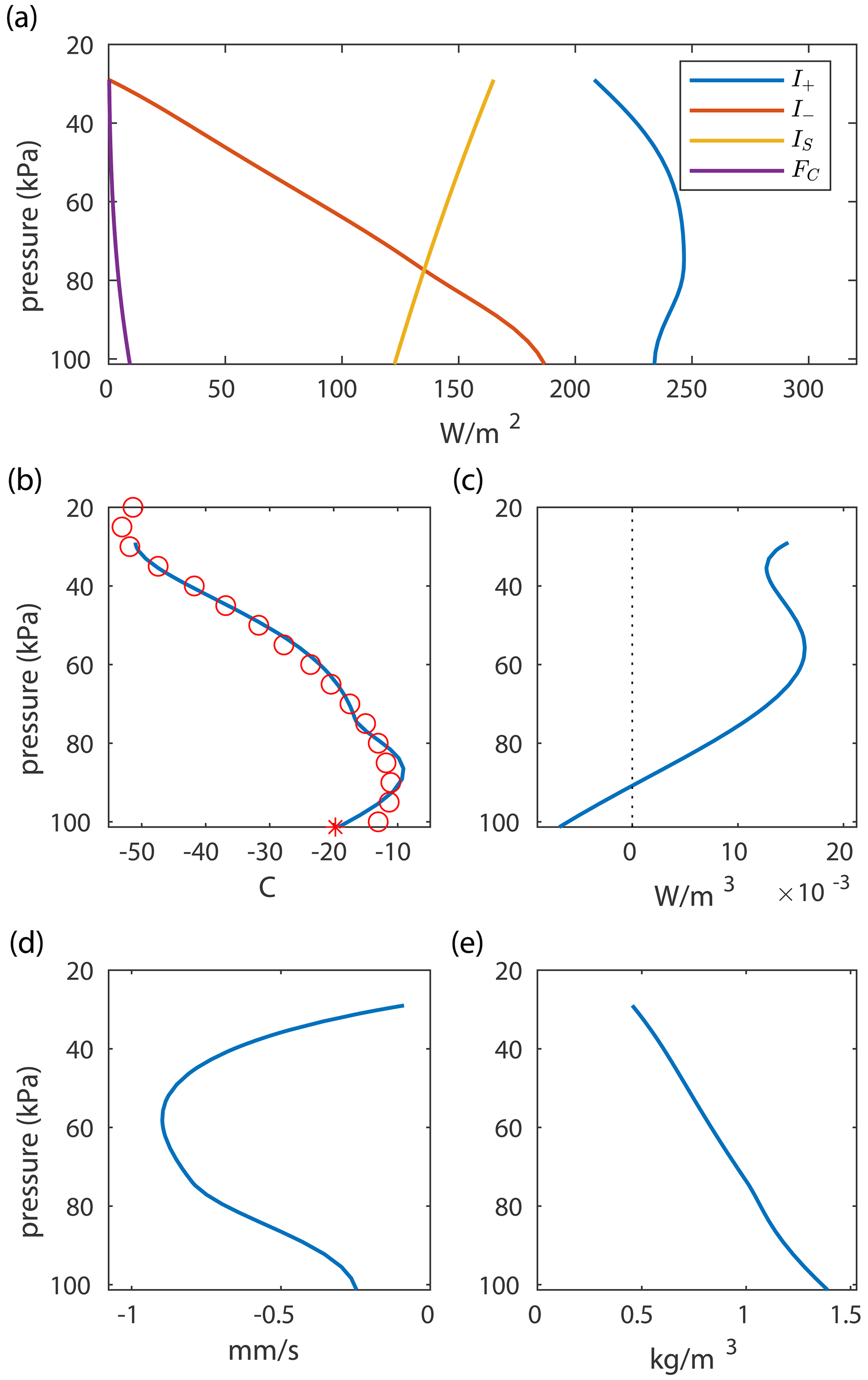
Figure 3 Results of the fully calibrated Arctic model at μ=390 ppm. The vertical axis in all the plots is the pressure. (a) Energy transport via radiative terms, and latent and sensible heat. (b) Temperature of the atmosphere. The red circles are the data from Cronin and Jansen (2016). The red asterisk is the surface temperature, T_S. (c) Atmospheric heat transport, F_A. (d) Vertical wind speed. (e) Density.

For μ=390, the surface temperature from the solved model is −19.7 ^∘C. Starting from this solution, we numerically continued the solution to other values of μ, resulting in the S-shaped curve in Fig. 4a. Between approximately μ=464 and μ=859, there are three solutions. The lower and upper solutions are stable cold and warm solutions, while the middle branch is unstable. Currently the Arctic is on the cold branch of this curve. The model predicts that, as CO₂ levels rise, the equilibrium surface temperature in the Arctic will increase gradually at first. However, when μ exceeds 859 ppm, the model displays a saddle-node bifurcation where the stable cold solution is annihilated together with the unstable solution. At this point the climate would rapidly approach the warm stable solution where surface temperatures are significantly higher. The temperatures on the warm branch may seem unreasonably high. Although our model includes specific details of some of the natural phenomena governing the Arctic climate behaviour and is calibrated with real data, it is primarily a qualitative rather than quantitative model. It is the fact that the model predicts the qualitative feature of a saddle-node bifurcation that is the important result, not the precise temperature of the model's warm solution. Part of the reason the model has relatively high temperatures on the warm branch is because it has constant values for F_O and $F_{\mathrm{A}}^{\mathrm{tot}}$. It is likely that, should the Arctic's annually averaged temperature rise dramatically, both F_O and $F_{\mathrm{A}}^{\mathrm{tot}}$ would be affected in a downward direction, which would reduce the warm equilibrium temperatures to some degree. Another important emergent feature of the model is that there is bistability for μ in the range [464,859]. Thus, even though the Arctic may in the future be on the cold branch in this range, it is possible that a strong enough climate disturbance could push the climate out of the basin of attraction of the cold solution and into the basin of attraction of the warm solution. The necessary strength of such a disturbance decreases as one moves closer to the upper end of this range. Our model does not incorporate the seasonal variation of solar input to the Arctic but rather uses an annually averaged value. Thus the equilibria in our model are annual averages. The seasonal variation of insolation would effectively result in oscillations around the annual average. These oscillations themselves may make a significant contribution to the “disturbance” needed to push the system out of the basin of attraction of the cold branch.

Figure 4 (a) Model surface temperature as a function of CO₂ concentration, μ. (b) CO₂ concentration levels for RCPs 2.6, 4.5, 6.0, and 8.5 (left to right). The dashed lines in panel (a) correspond to the CO₂ concentration levels for the four RCPs in the year 2200. The dashed-dotted line extends from the bifurcation point in panel (a) to RCP8.5 in the lower panel, indicating the bifurcation occurs in approximately the year 2100 for this scenario. The inset shows the predicted surface temperature as a function of the year for the four RCPs.

The International Panel on Climate Change (IPCC) has published various CO₂ emission scenarios for the future based on possible levels of global action to suppress such emissions (Intergovernmental Panel on Climate Change, 2013, Box TS.6; van Vuuren et al., 2011). These scenarios are called Representative Concentration Pathways (RCPs) and are numbered based on the radiative forcing in the year 2100 due to anthropogenic emissions compared to the year 1750. The original four published RCPs are RCP2.6, RCP4.5, RCP6.0, and RCP8.5, representing strong mitigation (2.6) through “ignore the problem” (8.5) responses by world governments. Each RCP indicates likely CO₂ concentration levels in the atmosphere out to the year 2100. From 2100 to 2200, the scenarios assume a “constant composition commitment”, which essentially freezes emission levels and eventually leads to a constant CO₂ level in the atmosphere for all but RCP8.5. These RCPs are plotted in Fig. 4b. The CO₂ levels for the four different pathways at the year 2200 are continued as dashed lines into Fig. 4a. It is clear from the figure that RCP8.5 leads to CO₂ concentrations that far surpass the saddle-node bifurcation, whereas the other three RCPs do not. This result is in agreement with our simpler model (Kypke et al., 2020). Both RCP6.0 and RCP4.5 end at levels within the bistable range, and indeed all the RCPs except RCP2.6 are within that range from about the year 2050 onward. The black dashed-dotted line extending from the bifurcation in the upper panel to RCP8.5 in the lower panel illustrates that RCP8.5 reaches the bifurcation near the year 2092.

The curve of equilibria in Fig. 4a displays hysteresis: CO₂ levels rising past 859 ppm will cause a jump from the cold equilibrium state to the warm state, but a return to the cold state will not happen until CO₂ levels are brought below 464 ppm, where the saddle-node bifurcation of the warm equilibrium is located (left bend of the S curve). If CO₂ levels follow a trajectory similar to RCP8.5, Arctic climate may change drastically in less than 100 years, but a return to the current cold state may be essentially impossible for thousands of years afterward, assuming humankind can develop and implement the required technology to reduce atmospheric carbon levels sufficiently.

Total atmospheric heat transport, $F_{\mathrm{A}}^{\mathrm{tot}}$, and ocean heat transport, F_O, are inputs to the model that are empirically based and that are not altered by the state of the model itself. We investigated the persistence of the saddle-node bifurcation and hysteresis in the presence of the uncertainty of these two values. Figure 5 shows two 2D bifurcation diagrams plotting the locations of the saddle-node bifurcations in the model (the left and right bends of the S curve in Fig. 4). Figure 5a shows the bifurcations as both $F_{\mathrm{A}}^{\mathrm{tot}}$ and μ vary. Figure 5b shows a similar diagram where F_O replaces $F_{\mathrm{A}}^{\mathrm{tot}}$. The right curve in each of the panels is a curve of saddle-node bifurcations corresponding to the right bend in the S curve in Fig. 4; they are transitions from a cold state to a warm state. Similarly, the left curve in each of the panels is a curve of saddle-node bifurcations that correspond to the left bend in the S curve and are the transitions from a warm state to a cold state. The shaded area between the two curves is the region of bistability. The curves meet in a cusp bifurcation, but it is important to note that this only occurs when CO₂ levels are mathematically negative. Thus the two saddle-node bifurcations and the hysteresis phenomenon will be present for all physically possible CO₂ levels and for all reasonable values of $F_{\mathrm{A}}^{\mathrm{tot}}$ and F_O. These bifurcation curves also make it evident that a transition from a cold state to a warm state occurs if either $F_{\mathrm{A}}^{\mathrm{tot}}$ or F_O are increased, even if CO₂ levels are constant. If $F_{\mathrm{A}}^{\mathrm{tot}}$ and F_O increase along with carbon dioxide levels in the near future, which seems reasonably likely, then the saddle-node bifurcation will occur at lower levels of CO₂. For example, a 10 % increase in $F_{\mathrm{A}}^{\mathrm{tot}}$ to 110 W m⁻² from 100 would cause the saddle-node bifurcation to occur at about μ=754 ppm, which would mean that both RCP8.5 and RCP6.0 would pass through the saddle-node bifurcation.

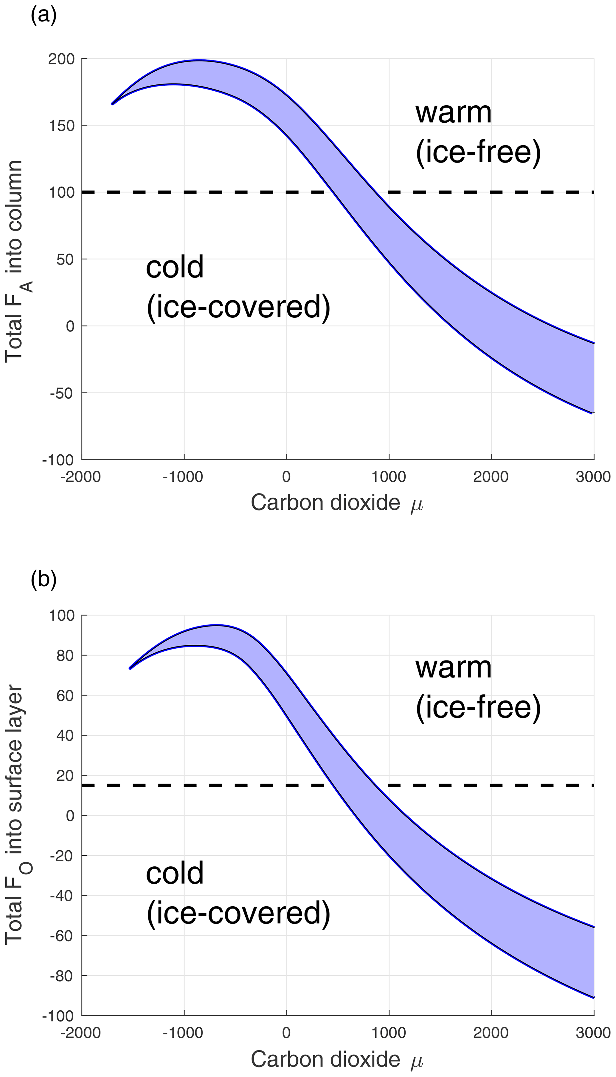
Figure 5 (a) Bifurcation diagram showing locations of saddle-node bifurcations as $F_{\mathrm{A}}^{\mathrm{tot}}$ and μ are varied. The dashed line indicates the value of $F_{\mathrm{A}}^{\mathrm{tot}}$ used in the model. The shaded area between the curves is the region of bistability. Abrupt transition from a cold state to a warm state occurs on the right curve, while abrupt transition from a warm state to a cold state occurs on the left curve. (b) Same except F_O is the varying parameter on the vertical axis rather than $F_{\mathrm{A}}^{\mathrm{tot}}$.

4 Conclusions

Although the model presented here is clearly a simplification of the climate, made possible by the near invariance of the vertical flow on the polar axis, we believe it captures some of the most important aspects relevant for Arctic climate change. The model predicts that if humanity keeps carbon emission levels close to RCP6.0 or lower, then the Arctic will not likely undergo a sudden dramatic rise in annual average temperature. However, if carbon emissions are much worse than RCP6.0, such a change is likely, and the cause is a saddle-node bifurcation of the stable cold equilibrium. Such a change would clearly have catastrophic effects on the Arctic environment, leading to massive global effects. These results are in agreement with those of Årthun et al. (2021), who, from a study of various CMIP6 models of Arctic climate, predict that under a low emissions scenario sea ice loss will be seasonal but that for a high emissions scenario it will be year-round for all areas of the Arctic. Further, the hysteresis displayed by the model indicates that a change of this nature may be practically irreversible. Although some comfort may be taken that only the worst of the four carbon pathway scenarios ends in such a catastrophic change, the model shows that both RCP6.0 and RCP4.5 lie in the region of bistability from the year 2070 onward. In a bistable situation, external disturbances could cause the system to jump into the basin of attraction of the warm equilibrium, effectively bringing about the catastrophic change prior to the bifurcation. The model is too simple to allow for any reasonable measure of the likelihood of such an occurrence, but the important thing is that the model exhibits bistability in the parameter region where the system is likely to reside within 50 years' time. This bistability has been shown to persist regardless of the values of the two biggest uncertainties in the model, the atmospheric and ocean heat transport to the Arctic from the mid-latitudes.

Our model addresses the equilibrium state only and represents the Arctic temperature as an annual average. The real Arctic climate undergoes massive seasonal changes, which effectively means that the system is actually oscillating around the equilibrium temperatures of our model. Such temperature oscillations may be sufficient to effectively push a system located on a cold solution in the bistable regime to “above” the unstable solution and so into the basin of attraction of the warm solution.

Seasonal variations in Arctic temperatures and sea ice are studied in many works, including Eisenman and Wettlaufer (2009), who argue that a tipping point to a year-round ice-free Arctic is not likely to occur while the Arctic is ice-covered for a significant portion of the year, but once the Arctic is seasonally ice-free for a sufficient number of months in a year, such a tipping point becomes more likely. A possible enhancement to our model would be to include seasonal solar variation and an ice model as in Eisenman and Wettlaufer (2009).

Appendix A: Model derivation details

This Appendix provides details regarding the model. The model is written in a nondimensional form in Sect. A1, defining nondimensional variables and parameters. This system is then transformed in Sect. A2 to a standard form of nine first-order ordinary differential equations and corresponding boundary conditions. This standard form makes it evident that the system is numerically stiff due to the fact that the thermal conductivity, k, of air is very small. To remove this stiffness, the limit as k→0 is applied, which reduces the system by one dimension. Section A3 discusses our choice of the functional forms for the dependence of relative humidity δ(z), atmospheric meridional heat transport F_A(z), and mass flux M_b(z) on altitude.

A1 Nondimensionalization

Define the nondimensional variables

$$\begin{array}{llllll}{\displaystyle }\widehat{z}& {\displaystyle }={\displaystyle \frac{z-z_{\mathrm{B}}}{z_{\mathrm{T}}-z_{\mathrm{B}}}},& {\displaystyle }{y}_{\mathrm{1}}& {\displaystyle }={\displaystyle \frac{w{c}_v{\mathit{\rho }}_{\mathrm{0}}{T}_{\mathrm{R}}}{\mathit{\sigma }{T}_{\mathrm{R}}^{\mathrm{4}}}},& {\displaystyle }{y}_{\mathrm{2}}& {\displaystyle }={\displaystyle \frac{\mathit{\rho }}{{\mathit{\rho }}_{\mathrm{0}}}},\\ {\displaystyle }{y}_{\mathrm{3}}& {\displaystyle }={\displaystyle \frac{I_{+}}{\mathit{\sigma }{T}_{\mathrm{R}}^{\mathrm{4}}}},& {\displaystyle }{y}_{\mathrm{4}}& {\displaystyle }={\displaystyle \frac{I_{-}}{\mathit{\sigma }{T}_{\mathrm{R}}^{\mathrm{4}}}},& {\displaystyle }{y}_{\mathrm{5}}& {\displaystyle }={\displaystyle \frac{I_{\mathrm{S}}}{\mathit{\sigma }{T}_{\mathrm{R}}^{\mathrm{4}}}},\\ {\displaystyle }{y}_{\mathrm{6}}& {\displaystyle }={\displaystyle \frac{F_{\mathrm{C}}}{\mathit{\sigma }{T}_{\mathrm{R}}^{\mathrm{4}}}},& {\displaystyle }{y}_{\mathrm{7}}& {\displaystyle }={\displaystyle \frac{T}{T_{\mathrm{R}}}},\\ \text{(A1)}& {\displaystyle }{y}_{\mathrm{8}}& {\displaystyle }=\left({\displaystyle \frac{z_{\mathrm{T}}-z_{\mathrm{B}}}{T_{\mathrm{R}}}}\right){\displaystyle \frac{\mathrm{d}T}{\mathrm{d}z}},& {\displaystyle }{y}_{\mathrm{9}}& {\displaystyle }={\displaystyle \frac{T_{\mathrm{S}}}{T_{\mathrm{R}}}},\end{array}$$

where P₀ (N m⁻²) is the standard atmospheric pressure, T_R is the freezing point of water in Kelvin, ${\mathit{\rho }}_{\mathrm{0}}=P_{\mathrm{0}}/\left(R_{\mathrm{A}}{T}_{\mathrm{R}}\right)$ is the density at standard pressure and freezing temperature, and $\mathit{\sigma }{T}_{\mathrm{R}}^{\mathrm{4}}/\left(c_v{\mathit{\rho }}_{\mathrm{0}}{T}_{\mathrm{R}}\right)$ represents the vertical velocity required to move a parcel of air with standard density at freezing temperature so that the power transferred is equal to the radiative power for a black body at the same temperature. This comes to about 1 mm s⁻¹.

Applying the change in variables to the troposphere BVP, Eqs. (3)–(7), (10), (11), and (31), we get

$$\begin{array}{ll}\text{(A2)}& {\displaystyle \frac{\mathrm{d}}{\mathrm{d}\widehat{z}}}\left(y_{\mathrm{1}}{y}_{\mathrm{2}}\right)=& {\displaystyle }D\mathit{\varphi }\left(\widehat{z}\right),\text{(A3)}& {\displaystyle }H{\displaystyle \frac{\mathrm{d}}{\mathrm{d}\widehat{z}}}\left(y_{\mathrm{1}}^{\mathrm{2}}{y}_{\mathrm{2}}\right)=& {\displaystyle }-J{\displaystyle \frac{\mathrm{d}}{\mathrm{d}\widehat{z}}}\left(y_{\mathrm{2}}{y}_{\mathrm{7}}\right)-E{y}_{\mathrm{2}},\text{(A4)}& {\displaystyle \frac{\mathrm{d}{y}_{\mathrm{3}}}{\mathrm{d}\widehat{z}}}=& {\displaystyle }-\widehat{\mathit{\kappa }}(y_{\mathrm{2}},y_{\mathrm{7}})(y_{\mathrm{3}}-y_{\mathrm{7}}^{\mathrm{4}}),\text{(A5)}& {\displaystyle \frac{\mathrm{d}{y}_{\mathrm{4}}}{\mathrm{d}\widehat{z}}}=& {\displaystyle }\widehat{\mathit{\kappa }}(y_{\mathrm{2}},y_{\mathrm{7}})(y_{\mathrm{4}}-y_{\mathrm{7}}^{\mathrm{4}}),\text{(A6)}& {\displaystyle \frac{\mathrm{d}{y}_{\mathrm{5}}}{\mathrm{d}\widehat{z}}}=& {\displaystyle }{G}_{\mathrm{S}}{y}_{\mathrm{2}}{y}_{\mathrm{5}},\text{(A7)}& {\displaystyle \frac{\mathrm{d}{y}_{\mathrm{6}}}{\mathrm{d}\widehat{z}}}=& {\displaystyle }-B_{\mathrm{1}}{y}_{\mathrm{6}},\text{(A8)}& {\displaystyle \frac{\mathrm{d}{y}_{\mathrm{7}}}{\mathrm{d}\widehat{z}}}=& {\displaystyle }{y}_{\mathrm{8}},{\displaystyle }\mathit{ϵ}{\displaystyle \frac{\mathrm{d}{y}_{\mathrm{8}}}{\mathrm{d}\widehat{z}}}=& {\displaystyle }{\displaystyle \frac{\mathrm{d}}{\mathrm{d}\widehat{z}}}\left({\displaystyle \frac{H}{\mathrm{2}}}{y}_{\mathrm{1}}^{\mathrm{3}}{y}_{\mathrm{2}}+E{y}_{\mathrm{1}}{y}_{\mathrm{2}}\widehat{z}+y_{\mathrm{1}}{y}_{\mathrm{2}}{y}_{\mathrm{7}}\right)\\ {\displaystyle }& {\displaystyle }+J{\displaystyle \frac{\mathrm{d}}{\mathrm{d}\widehat{z}}}\left(y_{\mathrm{1}}{y}_{\mathrm{2}}{y}_{\mathrm{7}}\right)-DE\widehat{z}\mathit{\varphi }\left(\widehat{z}\right)-D\mathit{\varphi }\left(\widehat{z}\right)y_{\mathrm{7}}\\ {\displaystyle }& {\displaystyle }-\widehat{\mathit{\kappa }}(y_{\mathrm{2}},y_{\mathrm{7}})(y_{\mathrm{3}}+y_{\mathrm{4}}-\mathrm{2}{y}_{\mathrm{7}}^{\mathrm{4}})-G_{\mathrm{S}}{y}_{\mathrm{2}}{y}_{\mathrm{5}}\\ \text{(A9)}& {\displaystyle }& {\displaystyle }-B_{\mathrm{1}}{y}_{\mathrm{6}}-{\widehat{F}}_{\mathrm{A}}\left(\widehat{z}\right),\text{(A10)}& {\displaystyle \frac{\mathrm{d}{y}_{\mathrm{9}}}{\mathrm{d}\widehat{z}}}=& {\displaystyle }\mathrm{0},\end{array}$$

for $\widehat{z}\in [\mathrm{0},\mathrm{1}]$. The boundary conditions, Eqs. (22)–(30), become

$$\begin{array}{ll}\text{(A11)}& {\displaystyle }{y}_{\mathrm{1}}\left(\mathrm{0}\right)y_{\mathrm{2}}\left(\mathrm{0}\right)=& {\displaystyle }D{\mathrm{\Phi }}_{\mathrm{B}},\text{(A12)}& {\displaystyle }{y}_{\mathrm{2}}\left(\mathrm{0}\right)y_{\mathrm{7}}\left(\mathrm{0}\right)=& {\displaystyle }\mathrm{1},{\displaystyle }{y}_{\mathrm{3}}\left(\mathrm{0}\right)=& {\displaystyle }\left(y_{\mathrm{9}}\right(\mathrm{0}{)}^{\mathrm{4}}-y_{\mathrm{7}}\left(\mathrm{0}{)}^{\mathrm{4}}\right)e^{-\widehat{\mathit{\kappa }}\left(y_{\mathrm{2}}\right(\mathrm{0}),y_{\mathrm{7}}(\mathrm{0}\left)\right)\mathit{\zeta }}\\ \text{(A13)}& {\displaystyle }& {\displaystyle }+y_{\mathrm{7}}(\mathrm{0}{)}^{\mathrm{4}},\text{(A14)}& {\displaystyle }{y}_{\mathrm{6}}\left(\mathrm{0}\right)=& {\displaystyle }{\widehat{F}}_{\mathrm{C}\mathrm{0}}\left(y_{\mathrm{2}}\right(\mathrm{0}),y_{\mathrm{7}}(\mathrm{0}),y_{\mathrm{9}}(\mathrm{0}\left)\right)e^{-B_{\mathrm{1}}\mathit{\zeta }},{\displaystyle }\mathrm{0}=& {\displaystyle }F-y_{\mathrm{9}}(\mathrm{0}{)}^{\mathrm{4}}+(y_{\mathrm{4}}\left(\mathrm{0}\right)-y_{\mathrm{7}}\left(\mathrm{0}{)}^{\mathrm{4}}\right)e^{-\widehat{\mathit{\kappa }}\left(y_{\mathrm{2}}\right(\mathrm{0}),y_{\mathrm{7}}(\mathrm{0}\left)\right)\mathit{\zeta }}\\ {\displaystyle }& {\displaystyle }+y_{\mathrm{7}}(\mathrm{0}{)}^{\mathrm{4}}+y_{\mathrm{5}}(\mathrm{0}\left)e^{-G_{\mathrm{S}}{y}_{\mathrm{2}}\left(\mathrm{0}\right)\mathit{\zeta }}\right(\mathrm{1}-\widehat{\mathit{\alpha }}\left(y_{\mathrm{9}}\right(\mathrm{0}\left)\right))\\ \text{(A15)}& {\displaystyle }& {\displaystyle }-{\widehat{F}}_{\mathrm{C}\mathrm{0}}\left(y_{\mathrm{2}}\right(\mathrm{0}),y_{\mathrm{7}}(\mathrm{0}),y_{\mathrm{9}}(\mathrm{0}\left)\right),{\displaystyle }\mathrm{0}=& {\displaystyle }F-y_{\mathrm{3}}\left(\mathrm{0}\right)+y_{\mathrm{4}}\left(\mathrm{0}\right)+y_{\mathrm{5}}\left(\mathrm{0}\right)\\ {\displaystyle }& {\displaystyle }-y_{\mathrm{5}}\left(\mathrm{0}\right)e^{-G_{\mathrm{S}}{y}_{\mathrm{2}}\left(\mathrm{0}\right)\mathit{\zeta }}\widehat{\mathit{\alpha }}\left(y_{\mathrm{9}}\right(\mathrm{0}\left)\right)-y_{\mathrm{6}}\left(\mathrm{0}\right)+\mathit{ϵ}{y}_{\mathrm{8}}\left(\mathrm{0}\right)\\ \text{(A16)}& {\displaystyle }& {\displaystyle }-{\displaystyle \frac{\mathrm{1}}{\mathrm{2}}}HD{\mathrm{\Phi }}_{\mathrm{B}}{y}_{\mathrm{1}}(\mathrm{0}{)}^{\mathrm{2}}-{\displaystyle \frac{\mathrm{1}}{\mathrm{2}}}DE{\mathrm{\Phi }}_{\mathrm{B}}\mathit{\zeta },\text{(A17)}& {\displaystyle }{y}_{\mathrm{4}}\left(\mathrm{1}\right)=& {\displaystyle }\mathrm{0},\text{(A18)}& {\displaystyle }{y}_{\mathrm{5}}\left(\mathrm{1}\right)=& {\displaystyle }{K}_{\mathrm{S}},\text{(A19)}& {\displaystyle }{y}_{\mathrm{8}}\left(\mathrm{1}\right)=& {\displaystyle }\mathrm{0},\end{array}$$

where

$$\begin{array}{ll}{\displaystyle }{\widehat{F}}_{\mathrm{C}\mathrm{0}}(y_{\mathrm{2}},y_{\mathrm{7}},y_{\mathrm{9}})=& {\displaystyle }{B}_{\mathrm{2}}{y}_{\mathrm{2}}(y_{\mathrm{9}}-y_{\mathrm{7}})\\ {\displaystyle }& {\displaystyle }+{\displaystyle \frac{B_{\mathrm{3}}}{y_{\mathrm{7}}}}[\exp \left(G_{\mathrm{W}\mathrm{1}}\left(\mathrm{1}-{\displaystyle \frac{\mathrm{1}}{y_{\mathrm{9}}}}\right)\right)\\ \text{(A20)}& {\displaystyle }& {\displaystyle }-\mathit{\delta }\left(\mathrm{0}\right)\exp \left(G_{\mathrm{W}\mathrm{1}}\left(\mathrm{1}-{\displaystyle \frac{\mathrm{1}}{y_{\mathrm{7}}}}\right)\right)],{\displaystyle }\widehat{\mathit{\kappa }}(y_{\mathrm{2}},y_{\mathrm{7}})=& {\displaystyle }\mathit{\kappa }(y_{\mathrm{2}}{\mathit{\rho }}_{\mathrm{0}},y_{\mathrm{7}}{T}_{\mathrm{R}})(z_{\mathrm{T}}-z_{\mathrm{B}})\\ {\displaystyle }=& {\displaystyle }{G}_{\mathrm{Cl}}+G_{\mathrm{C}}\widehat{\mathit{\mu }}{y}_{\mathrm{2}}\\ \text{(A21)}& {\displaystyle }& {\displaystyle }+{\displaystyle \frac{G_{\mathrm{W}\mathrm{2}}\mathit{\delta }\left(\widehat{z}\right)}{y_{\mathrm{7}}}}\exp \left(G_{\mathrm{W}\mathrm{1}}\left(\mathrm{1}-{\displaystyle \frac{\mathrm{1}}{y_{\mathrm{7}}}}\right)\right),\text{(A22)}& {\displaystyle }{\widehat{F}}_{\mathrm{A}}\left(\widehat{z}\right)=& {\displaystyle }{\displaystyle \frac{(z_{\mathrm{T}}-z_{\mathrm{B}})F_{\mathrm{A}}\left(\widehat{z}\right(z_{\mathrm{T}}-z_{\mathrm{B}})+z_{\mathrm{B}})}{\mathit{\sigma }{T}_{\mathrm{R}}^{\mathrm{4}}}},{\displaystyle }\widehat{\mathit{\alpha }}\left(y_{\mathrm{9}}\right)=& {\displaystyle }{\displaystyle \frac{\mathrm{1}}{\mathrm{2}}}\left[\right({\mathit{\alpha }}_{\mathrm{w}}+{\mathit{\alpha }}_{\mathrm{c}})\\ \text{(A23)}& {\displaystyle }& {\displaystyle }+({\mathit{\alpha }}_{\mathrm{w}}-{\mathit{\alpha }}_{\mathrm{c}})\tanh \left({\displaystyle \frac{y_{\mathrm{9}}-\mathrm{1}}{\mathit{\omega }}}\right)],\end{array}$$

are nondimensionalized functions describing the sensible/latent heat flux from the surface, the absorption of longwave radiation due to greenhouse gases, the atmospheric heat transport, and the surface albedo, and α_w, α_c, ω, Φ_B, and

$$\begin{array}{llll}{\displaystyle }{B}_{\mathrm{1}}& {\displaystyle }=b(z_{\mathrm{T}}-z_{\mathrm{B}}),& {\displaystyle }{B}_{\mathrm{2}}& {\displaystyle }={\displaystyle \frac{c_v{\mathit{\rho }}_{\mathrm{0}}{C}_{\mathrm{D}}U}{\mathit{\sigma }{T}_{\mathrm{R}}^{\mathrm{3}}}},\\ {\displaystyle }{B}_{\mathrm{3}}& {\displaystyle }={\displaystyle \frac{{\mathit{\rho }}_{\mathrm{W}}^{\mathrm{sat}}\left(T_{\mathrm{R}}\right)C_{\mathrm{D}}U{L}_{\mathrm{v}}}{\mathit{\sigma }{T}_{\mathrm{R}}^{\mathrm{4}}}},& {\displaystyle }D& {\displaystyle }={\displaystyle \frac{M_{\mathrm{tot}}{c}_v}{\mathit{\sigma }{T}_{\mathrm{R}}^{\mathrm{3}}}},\\ {\displaystyle }E& {\displaystyle }={\displaystyle \frac{g(z_{\mathrm{T}}-z_{\mathrm{B}})}{c_v{T}_{\mathrm{R}}}},& {\displaystyle }F& {\displaystyle }={\displaystyle \frac{F_{\mathrm{O}}}{\mathit{\sigma }{T}_{\mathrm{R}}^{\mathrm{4}}}},\\ {\displaystyle }{G}_{\mathrm{Cl}}& {\displaystyle }=k_{\mathrm{Cl}}(z_{\mathrm{T}}-z_{\mathrm{B}}),& {\displaystyle }{G}_{\mathrm{C}}& {\displaystyle }=k_{\mathrm{C}}{\displaystyle \frac{M_{{\mathrm{CO}}_{\mathrm{2}}}}{M_{\mathrm{A}}}}{\mathit{\rho }}_{\mathrm{0}}(z_{\mathrm{T}}-z_{\mathrm{B}}),\\ {\displaystyle }{G}_{\mathrm{W}\mathrm{1}}& {\displaystyle }={\displaystyle \frac{L_{\mathrm{v}}}{R_{\mathrm{W}}{T}_{\mathrm{R}}}},& {\displaystyle }{G}_{\mathrm{W}\mathrm{2}}& {\displaystyle }=k_{\mathrm{W}}{\mathit{\rho }}_{\mathrm{W}}^{\mathrm{sat}}\left(T_{\mathrm{R}}\right)(z_{\mathrm{T}}-z_{\mathrm{B}}),\\ {\displaystyle }{G}_{\mathrm{S}}& {\displaystyle }=k_{\mathrm{S}}{\mathit{\rho }}_{\mathrm{0}}(z_{\mathrm{T}}-z_{\mathrm{B}}),& {\displaystyle }H& {\displaystyle }={\displaystyle \frac{{\mathit{\sigma }}^{\mathrm{2}}{T}_{\mathrm{R}}^{\mathrm{5}}}{c_v^{\mathrm{3}}{\mathit{\rho }}_{\mathrm{0}}^{\mathrm{2}}}},\\ {\displaystyle }J& {\displaystyle }={\displaystyle \frac{R_{\mathrm{A}}}{c_v}},& {\displaystyle }{K}_{\mathrm{S}}& {\displaystyle }={\displaystyle \frac{Q-Q_{\mathrm{R}}}{\mathit{\sigma }{T}_{\mathrm{R}}^{\mathrm{4}}}},\\ {\displaystyle }\mathit{ϵ}& {\displaystyle }={\displaystyle \frac{k}{(z_{\mathrm{T}}-z_{\mathrm{B}})\mathit{\sigma }{T}_{\mathrm{R}}^{\mathrm{3}}}},& {\displaystyle }\widehat{\mathit{\mu }}& {\displaystyle }={\displaystyle \frac{\mathit{\mu }}{{\mathrm{10}}^{\mathrm{6}}}},\\ \text{(A24)}& {\displaystyle }\mathit{\zeta }& {\displaystyle }={\displaystyle \frac{z_{\mathrm{B}}}{z_{\mathrm{T}}-z_{\mathrm{B}}}},\end{array}$$

are nondimensional constants. Values of the physical parameters are given in the tables in Appendix B. It turns out that all of the above nondimensional constants are close to order 1 (range 0.04 to 26) except $\mathit{\zeta }=\mathrm{5.6}\times {\mathrm{10}}^{-\mathrm{3}}$, which is the relative boundary layer thickness, $\mathit{ϵ}=\mathrm{2.35}\times {\mathrm{10}}^{-\mathrm{6}}$, which is the nondimensional conductance, and $H=\mathrm{7.96}\times {\mathrm{10}}^{-\mathrm{12}}$, which is a factor in the kinetic energy term. As shown in the next section, the fact that ϵ is small causes system stiffness.

A2 Standard form and vanishing conduction limit

The BVP given by Eqs. (A2)–(A19) contains derivatives of products of some of the variables. It can be put in standard ODE form via algebraic manipulations. First we expand the derivative on the left-hand side of Eq. (A3) and use Eq. (A2) to simplify it:

$$\begin{array}{ll}{\displaystyle \frac{\mathrm{d}}{\mathrm{d}\widehat{z}}}\left(y_{\mathrm{1}}^{\mathrm{2}}{y}_{\mathrm{2}}\right)& {\displaystyle }=y_{\mathrm{1}}{\displaystyle \frac{\mathrm{d}}{\mathrm{d}\widehat{z}}}\left(y_{\mathrm{1}}{y}_{\mathrm{2}}\right)+\left(y_{\mathrm{1}}{y}_{\mathrm{2}}\right){\displaystyle \frac{\mathrm{d}{y}_{\mathrm{1}}}{\mathrm{d}\widehat{z}}}\\ {\displaystyle }& {\displaystyle }=y_{\mathrm{1}}D\mathit{\varphi }\left(\widehat{z}\right)+y_{\mathrm{1}}{y}_{\mathrm{2}}{\displaystyle \frac{\mathrm{d}{y}_{\mathrm{1}}}{\mathrm{d}\widehat{z}}}.\end{array}$$

Thus, Eq. (A3) may be replaced with

$$\begin{array}{}\text{(A25)}& H{y}_{\mathrm{1}}{y}_{\mathrm{2}}{\displaystyle \frac{\mathrm{d}{y}_{\mathrm{1}}}{\mathrm{d}\widehat{z}}}+J{y}_{\mathrm{7}}{\displaystyle \frac{\mathrm{d}{y}_{\mathrm{2}}}{\mathrm{d}\widehat{z}}}=-J{y}_{\mathrm{2}}{y}_{\mathrm{8}}-HD{y}_{\mathrm{1}}\mathit{\varphi }\left(\widehat{z}\right)-E{y}_{\mathrm{2}},\end{array}$$

where we have used Eq. (A8) to replace the derivative of y₇. We can also expand the derivative in Eq. (A2) to get the equivalent equation

$$\begin{array}{}\text{(A26)}& y_{\mathrm{2}}{\displaystyle \frac{\mathrm{d}{y}_{\mathrm{1}}}{\mathrm{d}\widehat{z}}}+y_{\mathrm{1}}{\displaystyle \frac{\mathrm{d}{y}_{\mathrm{2}}}{\mathrm{d}\widehat{z}}}=D\mathit{\varphi }\left(\widehat{z}\right).\end{array}$$

Equations (A25) and (A26) are a linear system in $\mathrm{d}{y}_{\mathrm{1}}/\mathrm{d}\widehat{z}$ and $\mathrm{d}{y}_{\mathrm{2}}/\mathrm{d}\widehat{z}$, namely

$$\left[\begin{array}{cc}H{y}_{\mathrm{1}}{y}_{\mathrm{2}}& J{y}_{\mathrm{7}}\\ y_{\mathrm{2}}& y_{\mathrm{1}}\end{array}\right]\left[\begin{array}{c}\frac{\mathrm{d}{y}_{\mathrm{1}}}{\mathrm{d}\widehat{z}}\\ \frac{\mathrm{d}{y}_{\mathrm{2}}}{\mathrm{d}\widehat{z}}\end{array}\right]=\left[\begin{array}{c}-J{y}_{\mathrm{2}}{y}_{\mathrm{8}}-HD{y}_{\mathrm{1}}\mathit{\varphi }\left(\widehat{z}\right)-E{y}_{\mathrm{2}}\\ D\mathit{\varphi }\left(\widehat{z}\right)\end{array}\right].$$

Solving this yields

$$\begin{array}{}\text{(A27)}& {\displaystyle \frac{\mathrm{d}{y}_{\mathrm{1}}}{\mathrm{d}\widehat{z}}}& {\displaystyle }={\displaystyle \frac{(J{y}_{\mathrm{7}}+H{y}_{\mathrm{1}}^{\mathrm{2}})D\mathit{\varphi }\left(\widehat{z}\right)+y_{\mathrm{1}}{y}_{\mathrm{2}}(E+J{y}_{\mathrm{8}})}{y_{\mathrm{2}}(J{y}_{\mathrm{7}}-H{y}_{\mathrm{1}}^{\mathrm{2}})}},\text{(A28)}& {\displaystyle \frac{\mathrm{d}{y}_{\mathrm{2}}}{\mathrm{d}\widehat{z}}}& {\displaystyle }=-{\displaystyle \frac{\mathrm{2}H{y}_{\mathrm{1}}D\mathit{\varphi }\left(\widehat{z}\right)+y_{\mathrm{2}}(E+J{y}_{\mathrm{8}})}{J{y}_{\mathrm{7}}-H{y}_{\mathrm{1}}^{\mathrm{2}}}}.\end{array}$$

Now expanding the derivatives on the right-hand side of Eq. (A7) and simplifying, we obtain

$$\begin{array}{ll}{\displaystyle }\mathit{ϵ}{\displaystyle \frac{\mathrm{d}{y}_{\mathrm{8}}}{\mathrm{d}\widehat{z}}}=& {\displaystyle }\left[H{\displaystyle \frac{y_{\mathrm{1}}^{\mathrm{2}}}{\mathrm{2}}}+{\displaystyle \frac{J^{\mathrm{2}}{y}_{\mathrm{7}}^{\mathrm{2}}+H^{\mathrm{2}}{y}_{\mathrm{1}}^{\mathrm{4}}}{J{y}_{\mathrm{7}}-H{y}_{\mathrm{1}}^{\mathrm{2}}}}\right]D\mathit{\varphi }\left(\widehat{z}\right)+(J+\mathrm{1})y_{\mathrm{1}}{y}_{\mathrm{2}}{y}_{\mathrm{8}}\\ {\displaystyle }& {\displaystyle }+J{y}_{\mathrm{1}}{y}_{\mathrm{2}}{\displaystyle \frac{E{y}_{\mathrm{7}}+H{y}_{\mathrm{1}}^{\mathrm{2}}{y}_{\mathrm{8}}}{J{y}_{\mathrm{7}}-H{y}_{\mathrm{1}}^{\mathrm{2}}}}\\ {\displaystyle }& {\displaystyle }-\widehat{\mathit{\kappa }}(y_{\mathrm{2}},y_{\mathrm{7}})y_{\mathrm{2}}(y_{\mathrm{3}}+y_{\mathrm{4}}-\mathrm{2}{y}_{\mathrm{7}}^{\mathrm{4}})-G_{\mathrm{S}}{y}_{\mathrm{2}}{y}_{\mathrm{5}}\\ \text{(A29)}& {\displaystyle }& {\displaystyle }-B_{\mathrm{1}}{y}_{\mathrm{6}}-{\widehat{F}}_{\mathrm{A}}\left(\widehat{z}\right).\end{array}$$

In summary, the BVP for the troposphere in standard form is given by

$$\begin{array}{ll}\text{(A30)}& {\displaystyle \frac{\mathrm{d}{y}_{\mathrm{1}}}{\mathrm{d}\widehat{z}}}=& {\displaystyle }{\displaystyle \frac{(J{y}_{\mathrm{7}}+H{y}_{\mathrm{1}}^{\mathrm{2}})D\mathit{\varphi }\left(\widehat{z}\right)+y_{\mathrm{1}}{y}_{\mathrm{2}}(E+J{y}_{\mathrm{8}})}{y_{\mathrm{2}}(J{y}_{\mathrm{7}}-H{y}_{\mathrm{1}}^{\mathrm{2}})}},\text{(A31)}& {\displaystyle \frac{\mathrm{d}{y}_{\mathrm{2}}}{\mathrm{d}\widehat{z}}}=& {\displaystyle }-{\displaystyle \frac{\mathrm{2}H{y}_{\mathrm{1}}D\mathit{\varphi }\left(\widehat{z}\right)+y_{\mathrm{2}}(E+J{y}_{\mathrm{8}})}{J{y}_{\mathrm{7}}-H{y}_{\mathrm{1}}^{\mathrm{2}}}}\text{(A32)}& {\displaystyle \frac{\mathrm{d}{y}_{\mathrm{3}}}{\mathrm{d}\widehat{z}}}=& {\displaystyle }-\widehat{\mathit{\kappa }}(y_{\mathrm{2}},y_{\mathrm{7}})(y_{\mathrm{3}}-y_{\mathrm{7}}^{\mathrm{4}}),\text{(A33)}& {\displaystyle \frac{\mathrm{d}{y}_{\mathrm{4}}}{\mathrm{d}\widehat{z}}}=& {\displaystyle }\widehat{\mathit{\kappa }}(y_{\mathrm{2}},y_{\mathrm{7}})(y_{\mathrm{4}}-y_{\mathrm{7}}^{\mathrm{4}}),\text{(A34)}& {\displaystyle \frac{\mathrm{d}{y}_{\mathrm{5}}}{\mathrm{d}\widehat{z}}}=& {\displaystyle }{G}_{\mathrm{S}}{y}_{\mathrm{2}}{y}_{\mathrm{5}},\text{(A35)}& {\displaystyle \frac{\mathrm{d}{y}_{\mathrm{6}}}{\mathrm{d}\widehat{z}}}=& {\displaystyle }-B_{\mathrm{1}}{y}_{\mathrm{6}},\text{(A36)}& {\displaystyle \frac{\mathrm{d}{y}_{\mathrm{7}}}{\mathrm{d}\widehat{z}}}=& {\displaystyle }{y}_{\mathrm{8}},{\displaystyle }\mathit{ϵ}{\displaystyle \frac{\mathrm{d}{y}_{\mathrm{8}}}{\mathrm{d}\widehat{z}}}=& {\displaystyle }\left[H{\displaystyle \frac{y_{\mathrm{1}}^{\mathrm{2}}}{\mathrm{2}}}+{\displaystyle \frac{J^{\mathrm{2}}{y}_{\mathrm{7}}^{\mathrm{2}}+H^{\mathrm{2}}{y}_{\mathrm{1}}^{\mathrm{4}}}{J{y}_{\mathrm{7}}-H{y}_{\mathrm{1}}^{\mathrm{2}}}}\right]D\mathit{\varphi }\left(\widehat{z}\right)+(J+\mathrm{1})y_{\mathrm{1}}{y}_{\mathrm{2}}{y}_{\mathrm{8}}\\ {\displaystyle }& {\displaystyle }+J{y}_{\mathrm{1}}{y}_{\mathrm{2}}{\displaystyle \frac{E{y}_{\mathrm{7}}+H{y}_{\mathrm{1}}^{\mathrm{2}}{y}_{\mathrm{8}}}{J{y}_{\mathrm{7}}-H{y}_{\mathrm{1}}^{\mathrm{2}}}}-\widehat{\mathit{\kappa }}(y_{\mathrm{2}},y_{\mathrm{7}})(y_{\mathrm{3}}+y_{\mathrm{4}}-\mathrm{2}{y}_{\mathrm{7}}^{\mathrm{4}})\\ \text{(A37)}& {\displaystyle }& {\displaystyle }-G_{\mathrm{S}}{y}_{\mathrm{2}}{y}_{\mathrm{5}}-B_{\mathrm{1}}{y}_{\mathrm{6}}-{\widehat{F}}_{\mathrm{A}}\left(\widehat{z}\right),\text{(A38)}& {\displaystyle \frac{\mathrm{d}{y}_{\mathrm{9}}}{\mathrm{d}\widehat{z}}}=& {\displaystyle }\mathrm{0},\end{array}$$

with boundary conditions

$$\begin{array}{ll}\text{(A39)}& {\displaystyle }{y}_{\mathrm{1}}\left(\mathrm{0}\right)y_{\mathrm{2}}\left(\mathrm{0}\right)=& {\displaystyle }D{\mathrm{\Phi }}_{\mathrm{B}},\text{(A40)}& {\displaystyle }{y}_{\mathrm{2}}\left(\mathrm{0}\right)y_{\mathrm{7}}\left(\mathrm{0}\right)=& {\displaystyle }\mathrm{1},{\displaystyle }{y}_{\mathrm{3}}\left(\mathrm{0}\right)=& {\displaystyle }\left(y_{\mathrm{9}}\right(\mathrm{0}{)}^{\mathrm{4}}-y_{\mathrm{7}}\left(\mathrm{0}{)}^{\mathrm{4}}\right)e^{-\widehat{\mathit{\kappa }}\left(y_{\mathrm{2}}\right(\mathrm{0}),y_{\mathrm{7}}(\mathrm{0}\left)\right)\mathit{\zeta }}\\ \text{(A41)}& {\displaystyle }& {\displaystyle }+y_{\mathrm{7}}(\mathrm{0}{)}^{\mathrm{4}},\text{(A42)}& {\displaystyle }{y}_{\mathrm{6}}\left(\mathrm{0}\right)=& {\displaystyle }{\widehat{F}}_{\mathrm{C}\mathrm{0}}\left(y_{\mathrm{2}}\right(\mathrm{0}),y_{\mathrm{7}}(\mathrm{0}),y_{\mathrm{9}}(\mathrm{0}\left)\right)e^{-B_{\mathrm{1}}\mathit{\zeta }},{\displaystyle }\mathrm{0}=& {\displaystyle }F-y_{\mathrm{9}}(\mathrm{0}{)}^{\mathrm{4}}+(y_{\mathrm{4}}\left(\mathrm{0}\right)-y_{\mathrm{7}}\left(\mathrm{0}{)}^{\mathrm{4}}\right)e^{-\widehat{\mathit{\kappa }}\left(y_{\mathrm{2}}\right(\mathrm{0}),y_{\mathrm{7}}(\mathrm{0}\left)\right)\mathit{\zeta }}\\ {\displaystyle }& {\displaystyle }+y_{\mathrm{7}}(\mathrm{0}{)}^{\mathrm{4}}+y_{\mathrm{5}}(\mathrm{0}\left)e^{-G_{\mathrm{S}}{y}_{\mathrm{2}}\left(\mathrm{0}\right)\mathit{\zeta }}\right(\mathrm{1}-\widehat{\mathit{\alpha }}\left(y_{\mathrm{9}}\right(\mathrm{0}\left)\right))\\ \text{(A43)}& {\displaystyle }& {\displaystyle }-{\widehat{F}}_{\mathrm{C}\mathrm{0}}\left(y_{\mathrm{2}}\right(\mathrm{0}),y_{\mathrm{7}}(\mathrm{0}),y_{\mathrm{9}}(\mathrm{0}\left)\right),{\displaystyle }\mathrm{0}=& {\displaystyle }F-y_{\mathrm{3}}\left(\mathrm{0}\right)+y_{\mathrm{4}}\left(\mathrm{0}\right)+y_{\mathrm{5}}\left(\mathrm{0}\right)\\ {\displaystyle }& {\displaystyle }-y_{\mathrm{5}}\left(\mathrm{0}\right)e^{-G_{\mathrm{S}}{y}_{\mathrm{2}}\left(\mathrm{0}\right)\mathit{\zeta }}\widehat{\mathit{\alpha }}\left(y_{\mathrm{9}}\right(\mathrm{0}\left)\right)-y_{\mathrm{6}}\left(\mathrm{0}\right)+\mathit{ϵ}{y}_{\mathrm{8}}\left(\mathrm{0}\right)\\ \text{(A44)}& {\displaystyle }& {\displaystyle }-{\displaystyle \frac{\mathrm{1}}{\mathrm{2}}}HD{\mathrm{\Phi }}_{\mathrm{B}}{y}_{\mathrm{1}}(\mathrm{0}{)}^{\mathrm{2}}-{\displaystyle \frac{\mathrm{1}}{\mathrm{2}}}DE{\mathrm{\Phi }}_{\mathrm{B}}\mathit{\zeta },\text{(A45)}& {\displaystyle }{y}_{\mathrm{4}}\left(\mathrm{1}\right)=& {\displaystyle }\mathrm{0},\text{(A46)}& {\displaystyle }{y}_{\mathrm{5}}\left(\mathrm{1}\right)=& {\displaystyle }{K}_{\mathrm{S}},\text{(A47)}& {\displaystyle }{y}_{\mathrm{8}}\left(\mathrm{1}\right)=& {\displaystyle }\mathrm{0}.\end{array}$$

As mentioned above, of the nondimensional constants, all are close to order 1 except $\mathit{\zeta }=\mathrm{5.6}\times {\mathrm{10}}^{-\mathrm{3}}$, $H=\mathrm{7.96}\times {\mathrm{10}}^{-\mathrm{12}}$, and $\mathit{ϵ}=\mathrm{2.3}\times {\mathrm{10}}^{-\mathrm{6}}$ (with z_T=9000). The constant ζ only appears in the boundary conditions. The constant H occurs in the system only in summations with other non-derivative terms; hence the fact that it is small only means that those terms contribute little. It does not cause stiffness. The relatively small value of the constant ϵ, however, does cause stiffness in Eq. (A37) of the system. Because ϵ is small, the variable y₈, which is the dimensionless rate of vertical temperature change $\mathrm{d}T/\mathrm{d}z$, will approach the y₈-nullcline very rapidly (which means at a very short z distance from either boundary). To simplify numerical computation, we take the limit as ϵ goes to zero, which is equivalent to saying that conduction is negligible. In this limit, Eq. (A37) is an algebraic expression from which we can isolate y₈:

$$\begin{array}{ll}{\displaystyle }{y}_{\mathrm{8}}\left(\widehat{z}\right)=& {\displaystyle }-\left[\left(H{\displaystyle \frac{y_{\mathrm{1}}^{\mathrm{2}}}{\mathrm{2}}}+{\displaystyle \frac{J^{\mathrm{2}}{y}_{\mathrm{7}}^{\mathrm{2}}+H^{\mathrm{2}}{y}_{\mathrm{1}}^{\mathrm{4}}}{J{y}_{\mathrm{7}}-H{y}_{\mathrm{1}}^{\mathrm{2}}}}\right)D\mathit{\varphi }\left(\widehat{z}\right)\right.\\ {\displaystyle }& {\displaystyle }+{\displaystyle \frac{EJ{y}_{\mathrm{1}}{y}_{\mathrm{2}}{y}_{\mathrm{7}}}{J{y}_{\mathrm{7}}-H{y}_{\mathrm{1}}^{\mathrm{2}}}}-G_{\mathrm{S}}{y}_{\mathrm{2}}{y}_{\mathrm{5}}\\ {\displaystyle }& {\displaystyle }-\widehat{\mathit{\kappa }}(y_{\mathrm{2}},y_{\mathrm{7}})(y_{\mathrm{3}}+y_{\mathrm{4}}-\mathrm{2}{y}_{\mathrm{7}}^{\mathrm{4}})-B{y}_{\mathrm{6}}\\ \text{(A48)}& {\displaystyle }& {\displaystyle }-\left.{\widehat{F}}_{\mathrm{A}}\left(\widehat{z}\right)\right]{\left[(J+\mathrm{1})y_{\mathrm{1}}{y}_{\mathrm{2}}+{\displaystyle \frac{JH{y}_{\mathrm{1}}^{\mathrm{3}}{y}_{\mathrm{2}}}{J{y}_{\mathrm{7}}-H{y}_{\mathrm{1}}^{\mathrm{2}}}}\right]}^{-\mathrm{1}}.\end{array}$$

With this expression for y₈, the system is reduced by eliminating Eq. (A37) and boundary condition Eq. (A47). Since y₁, the dimensionless vertical velocity, is a factor in the denominator, it is necessary that y₁ be nonzero throughout the atmosphere in order not to introduce a singularity. For this reason we select Φ_T>0, Φ_B<0, and ϕ such that it is nonnegative in the upper atmosphere and non-positive in the lower atmosphere.

A3 Modelling choices for functional forms

In this section we describe the various functional forms that we used for relative humidity, atmospheric heat transport, and mass flux. For the latter two, several different forms were tried, and these are detailed below. Calibration to empirical data, described in Appendix B, was used to select specific functional forms for the heat transport and mass flux.

A3.1 Relative humidity

The relative humidity is modelled as a linear function decreasing with altitude from a higher surface value, δ_B, to a lower value at the tropopause, δ_T. Specifically,

$$\begin{array}{}\text{(A49)}& \mathit{\delta }\left(\widehat{z}\right)={\mathit{\delta }}_{\mathrm{B}}(\mathrm{1}-\widehat{z})+{\mathit{\delta }}_{\mathrm{T}}\widehat{z}.\end{array}$$

A3.2 Atmospheric heat transport

Atmospheric heat transport is primarily due to large-scale turbulent mixing of the column with its environment. This mixing is not modelled explicitly, but, instead, it is incorporated into the model via the function F_A(z), which represents the thermal energy supplied to the column by turbulent mixing. The integral of F_A(z) over the atmosphere thickness represents the total atmospheric heat transport in/out of the system. So, given a set amount of such energy, $F_{\mathrm{A}}^{\mathrm{tot}}$, we have

$$\begin{array}{}\text{(A50)}& F_{\mathrm{A}}^{\mathrm{tot}}=\underset{z_{\mathrm{B}}}{\overset{z_{\mathrm{T}}}{\int }}{F}_{\mathrm{A}}\left(z\right)\mathrm{d}z=\mathit{\sigma }{T}_{\mathrm{R}}^{\mathrm{4}}\underset{\mathrm{0}}{\overset{\mathrm{1}}{\int }}{\widehat{F}}_{\mathrm{A}}\left(\widehat{z}\right)\mathrm{d}\widehat{z}.\end{array}$$

This provides one restriction on the function F_A(z), but its precise form is a modelling choice. However, the exact form must be chosen with care, because with certain choices of F_A(z), the boundary conditions can only be satisfied with unrealistic solutions. In particular, if the values of F_A(z) near the tropopause (z near z_T, that is, $\widehat{z}$ near 1) are too small, then the temperature drops precipitously toward absolute zero; if they are too big, the temperature turns around and climbs rapidly. Thus, in order to automate an appropriate choice of F_A(z), we have proceeded as follows.

1. Choose ${\widehat{F}}_{\mathrm{A}}\left(\mathrm{1}\right)$ such that the temperature gradient at the tropopause is zero, that is, re-impose boundary condition Eq. (A47). Thus use Eq. (A48) with y₈(1)=0 to solve for ${\widehat{F}}_{\mathrm{A}}\left(\mathrm{1}\right)$. Let ${\widehat{F}}_{\mathrm{A}\mathrm{1}}$ denote this value of ${\widehat{F}}_{\mathrm{A}}\left(\mathrm{1}\right)$, and let F_A1 denote the corresponding dimensional value of F_A(z_T), that is, $F_{\mathrm{A}\mathrm{1}}={\widehat{F}}_{\mathrm{A}\mathrm{1}}\mathit{\sigma }{T}_{\mathrm{R}}^{\mathrm{4}}/(z_{\mathrm{T}}-z_{\mathrm{B}})$.

2. Assume that F_A(z) is of the form

   $$\begin{array}{}\text{(A51)}& F_{\mathrm{A}}\left(z\right)=F_{\mathrm{Ab}}\left(z\right)+{\displaystyle \frac{F_{\mathrm{A}}^{\mathrm{tot}}}{z_{\mathrm{T}}-z_{\mathrm{B}}}}\mathit{\psi }\left({\displaystyle \frac{z-z_{\mathrm{B}}}{z_{\mathrm{T}}-z_{\mathrm{B}}}}\right),\end{array}$$

   where the base function F_Ab(z) is a linear function passing through zero at the midpoint of the atmosphere and equal to F_A1 at z_T, that is,

   $$\begin{array}{rl}& F_{\mathrm{Ab}}\left(z\right)=F_{\mathrm{A}\mathrm{1}}{\displaystyle \frac{\mathrm{2}z-(z_{\mathrm{T}}+z_{\mathrm{B}})}{z_{\mathrm{T}}-z_{\mathrm{B}}}},\\ & ⟺{\widehat{F}}_{\mathrm{Ab}}\left(\widehat{z}\right)={\widehat{F}}_{\mathrm{A}\mathrm{1}}(\mathrm{2}\widehat{z}-\mathrm{1}).\end{array}$$

   This base portion of F_A contributes no net heat to the column; it is simply a factor that essentially moves heat around in the column in order to ensure the temperature gradient at the top is zero.

   The remaining portion of F_A is the actual atmospheric heat transport entering the column from outside. We assume that $\mathit{\psi }\left(\widehat{z}\right)$ satisfies

   $${\displaystyle }\mathit{\psi }\left(\mathrm{1}\right)=\mathrm{0}\text{and}\underset{\mathrm{0}}{\overset{\mathrm{1}}{\int }}\mathit{\psi }\left(x\right)\mathrm{d}x=\mathrm{1},$$

   so that the value of F_A is not altered at the tropopause and so that $F_{\mathrm{A}}^{\mathrm{tot}}$ (W m⁻²) represents the total energy flux of atmospheric heat transport entering the column. Thus, the nondimensional function is

   $${\widehat{F}}_{\mathrm{A}}\left(\widehat{z}\right)={\widehat{F}}_{\mathrm{A}\mathrm{1}}(\mathrm{2}\widehat{z}-\mathrm{1})+{\widehat{F}}_{\mathrm{A}}^{\mathrm{tot}}\mathit{\psi }\left(\widehat{z}\right),$$

   where

   $${\widehat{F}}_{\mathrm{A}}^{\mathrm{tot}}={\displaystyle \frac{F_{\mathrm{A}}^{\mathrm{tot}}}{\mathit{\sigma }{T}_{\mathrm{R}}^{\mathrm{4}}}}.$$

3. As a numerical issue, since the boundary condition value ${\widehat{F}}_{\mathrm{A}\mathrm{1}}$ is needed in the computation of the vector field and since the MATLAB solver we are using does not have a way of making boundary condition information available to the vector field computation function, we circumvented this issue by adding another variable to the problem y₁₀, with differential equation $\mathrm{d}{y}_{\mathrm{10}}/\mathrm{d}\widehat{z}=\mathrm{0}$ and boundary condition $y_{\mathrm{10}}\left(\mathrm{1}\right)={\widehat{F}}_{\mathrm{A}\mathrm{1}}$.

4. The choice of the functional form of $\mathit{\psi }\left(\widehat{z}\right)$ is somewhat open, and we tested the following two forms:

   $$\begin{array}{}\text{(A52)}& {\displaystyle }\mathit{\psi }\left(\widehat{z}\right)& {\displaystyle }=g_{\mathrm{1}}(\mathrm{1}-\widehat{z},L_{\mathit{\psi }}),\text{(A53)}& {\displaystyle }\mathit{\psi }\left(\widehat{z}\right)& {\displaystyle }=g_{\mathrm{2}}(\mathrm{1}-\widehat{z},L_{\mathit{\psi }}),\end{array}$$

   where the functions g₁ and g₂ are defined as

   $$\begin{array}{ll}{\displaystyle }{g}_{\mathrm{1}}(x,L)=& {\displaystyle }{\displaystyle \frac{L\mathit{\pi }}{\mathrm{1}-\cos \left(L\mathit{\pi }\right)}}\sin \left(L\mathit{\pi }x\right),\\ \text{(A54)}& {\displaystyle }{g}_{\mathrm{2}}(x,L)=& {\displaystyle }{\displaystyle \frac{\mathrm{2}L\mathit{\pi }}{\mathrm{2}L\mathit{\pi }-\sin \left(\mathrm{2}L\mathit{\pi }\right)}}\left(\mathrm{1}-\cos \left(\mathrm{2}L\mathit{\pi }x\right)\right),\end{array}$$

   and where L is a parameter in (0,1] free to be chosen. (The functions g₁ and g₂ will also be utilized in the modelling of $\mathit{\varphi }\left(\widehat{z}\right)$.) The primary difference between these two forms is that the first has a non-zero slope at x=0, while the latter has a zero slope there.

A3.3 Mass flux

The function ϕ dictates the mass flux across the vertical boundary (negative outward), and, along with the fluxes Φ_B and Φ_T across the bottom and top of the column, drives the vertical air movement in the column. The only general restrictions on these fluxes are given by Eq. (2). To model the situation in the Arctic, we want a downward flow of air with a vertical wind speed, w, of the order of 1 mm s⁻¹ in the column. A reasonable assumption at the tropopause would be to set w=0; however, since our model has a singularity when w=0, we impose a small wind speed at the tropopause by ensuring Φ_T is positive. At the surface boundary layer we impose Φ_B≤0. Further, to simplify matters and to ensure a downward flow throughout the column, we assume that

$$\begin{array}{ll}{\displaystyle }\mathit{\varphi }\left(\widehat{z}\right)& {\displaystyle }\le \mathrm{0},\text{if}\widehat{z}\in [\mathrm{0},z_{\mathrm{c}}),\\ {\displaystyle }\mathit{\varphi }\left(\widehat{z}\right)& {\displaystyle }\ge \mathrm{0},\text{if}\widehat{z}\in [z_{\mathrm{c}},\mathrm{1}],\end{array}$$

where z_c is some point in [0,1]. The following forms were tested for $\mathit{\varphi }\left(\widehat{z}\right)$:

piecewise constant,

$$\begin{array}{}\text{(A55)}& \mathit{\varphi }\left(\widehat{z}\right)=\left\{\begin{array}{ll}\frac{-\mathrm{1}-{\mathrm{\Phi }}_B}{z_c}& \text{if}\widehat{z}\in [\mathrm{0},z_c),\\ \frac{\mathrm{1}-{\mathrm{\Phi }}_T}{\mathrm{1}-z_c}& \text{if}\widehat{z}\in [z_c,\mathrm{1}],\end{array}\right.\end{array}$$

piecewise linear,

$$\begin{array}{}\text{(A56)}& \mathit{\varphi }\left(\widehat{z}\right)=\left\{\begin{array}{ll}\frac{\mathrm{2}(-\mathrm{1}-{\mathrm{\Phi }}_{\mathrm{B}})}{z_{\mathrm{c}}^{\mathrm{2}}}\left(z_{\mathrm{c}}-\widehat{z}\right),& \text{if}\widehat{z}\in [\mathrm{0},z_{\mathrm{c}}),\\ \frac{\mathrm{2}(\mathrm{1}-{\mathrm{\Phi }}_{\mathrm{T}})}{(\mathrm{1}-z_{\mathrm{c}}{)}^{\mathrm{2}}}(\widehat{z}-z_{\mathrm{c}}),& \text{if}\widehat{z}\in [z_{\mathrm{c}},\mathrm{1}],\end{array}\right.\end{array}$$

piecewise sine,

$$\begin{array}{}\text{(A57)}& \mathit{\varphi }\left(\widehat{z}\right)=\left\{\begin{array}{ll}\frac{-\mathrm{1}-{\mathrm{\Phi }}_{\mathrm{B}}}{z_{\mathrm{c}}}{g}_{\mathrm{1}}\left(\mathrm{1}-\frac{\widehat{z}}{z_{\mathrm{c}}},L_{\mathit{\varphi }\mathrm{B}}\right),& \text{if}\widehat{z}\in [\mathrm{0},z_{\mathrm{c}}),\\ \frac{\mathrm{1}-{\mathrm{\Phi }}_{\mathrm{T}}}{\mathrm{1}-z_{\mathrm{c}}}{g}_{\mathrm{1}}\left(\frac{\widehat{z}-z_{\mathrm{c}}}{\mathrm{1}-z_{\mathrm{c}}},L_{\mathit{\varphi }\mathrm{T}}\right),& \text{if}\widehat{z}\in [z_{\mathrm{c}},\mathrm{1}],\end{array}\right.\end{array}$$

piecewise cosine,

$$\begin{array}{}\text{(A58)}& \mathit{\varphi }\left(\widehat{z}\right)=\left\{\begin{array}{ll}\frac{-\mathrm{1}-{\mathrm{\Phi }}_{\mathrm{B}}}{z_{\mathrm{c}}}{g}_{\mathrm{2}}\left(\mathrm{1}-\frac{\widehat{z}}{z_{\mathrm{c}}},L_{\mathit{\varphi }\mathrm{B}}\right),& \text{if}\widehat{z}\in [\mathrm{0},z_{\mathrm{c}}),\\ \frac{\mathrm{1}-{\mathrm{\Phi }}_{\mathrm{T}}}{\mathrm{1}-z_{\mathrm{c}}}{g}_{\mathrm{2}}\left(\frac{\widehat{z}-z_{\mathrm{c}}}{\mathrm{1}-z_{\mathrm{c}}},L_{\mathit{\varphi }\mathrm{T}}\right),& \text{if}\widehat{z}\in [z_{\mathrm{c}},\mathrm{1}],\end{array}\right.\end{array}$$

where g₁ and g₂ are defined by Eq. (A54). (In the case that z_c=0 or z_c=1, it is understood that only the non-empty interval for ϕ in the above definitions is used and that it is closed at both ends.)

Appendix B: Model parameters and calibration

This Appendix lists the parameter values used in the model and discusses how some of them were calibrated to empirical data. Section B2 gives the calculation of the average annual insolation for the Earth north of 70^∘ N.

B1 Parameter values and calibration

Values of the model parameters are given in Tables B1 and B2. The parameters in Table B1 are physical constants. The parameters in Table B2 are those that have been assigned from empirical data and knowledge or whose values have resulted from fitting the model to empirical data. The model was applied to the globally averaged situation for the purposes of calibration of some parameters (see below) and then also applied to the Arctic.

Table B1 Physical constants used in the model.

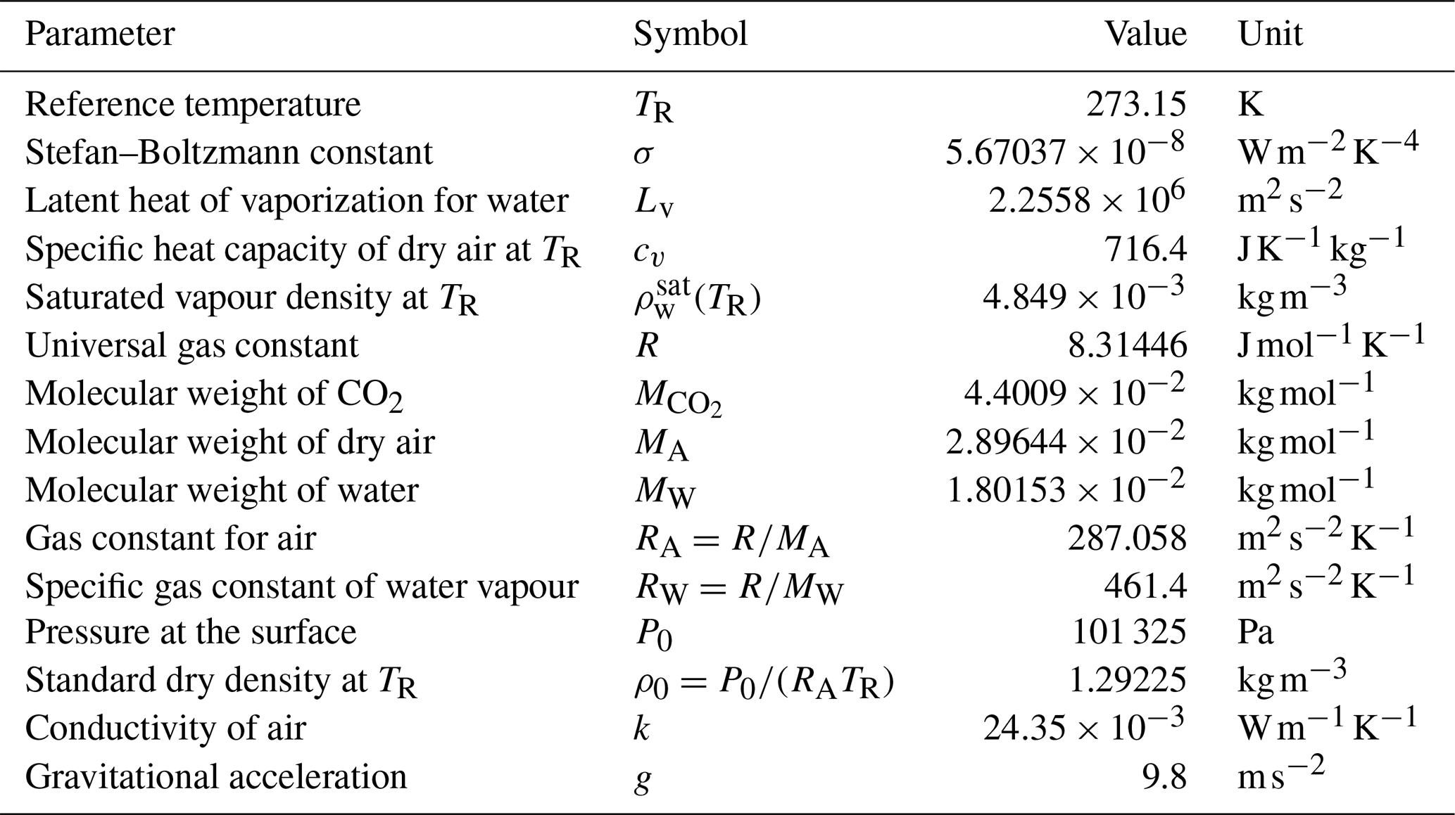
Table B2 Other model parameters. Some parameters are geographically dependent and have different values for the global and Arctic situations. An empty value in the “Arctic” column indicates the global value is used in both cases. Values that were fitted by the calibration steps described in the text are indicated in bold.

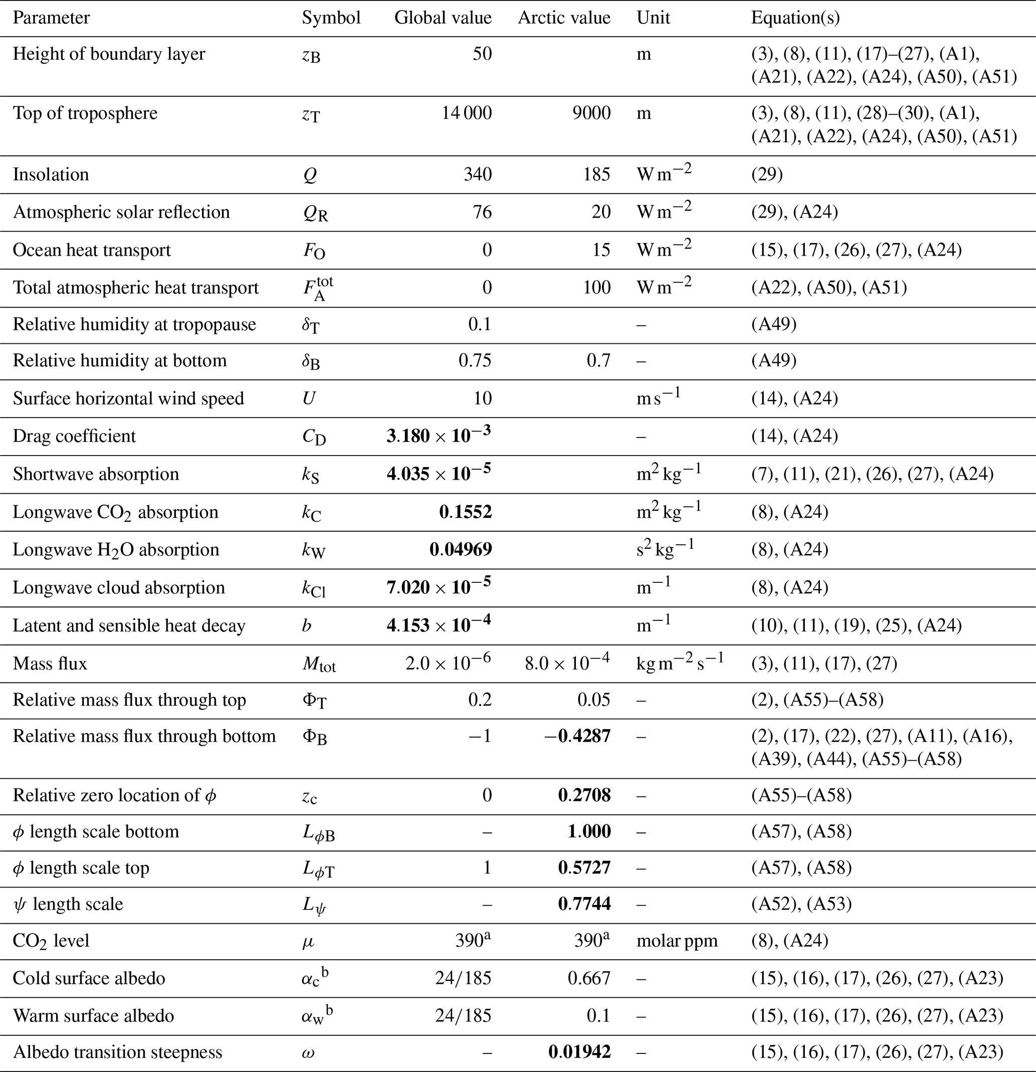
^a Values used for calibration only. ^b For the purposes of calibrating the model to global data, both α_c and α_w were set to the empirical value of $\mathrm{24}/\mathrm{185}$. When calibrating the model's mass flux and atmospheric heat transport parameters to Arctic data, both α_c and α_w were set to the empirical value of $\mathrm{2}/\mathrm{3}$.

Here we provide justification and explanation of our choice of parameter values in Table B2. The height of the boundary layer was set to z_B=50 m. The model is not very sensitive to this parameter. The height of the tropopause is about 9 km at the poles and 17 km at the Equator, so we used the lower value for the Arctic and a middle value of 14 km for the global average. The globally averaged insolation, the atmospheric solar reflection, and the average surface albedo are all obtained from Wild et al. (2013). For the Arctic, the insolation is the annual average for the region north of 70^∘ N, the calculation of which is shown in Sect. B2. For the average global situation, there is no ocean or atmospheric heat transport; the corresponding values for the Arctic come from Mayer et al. (2019) and Serreze et al. (2007). The Arctic atmospheric reflection and surface albedo come from Kalnay et al. (1996), National Centers for Environmental Protection/National Weather Service/NOAA/U.S. Department of Commerce (2021), and Mayer et al. (2019). Relative humidity is low at the top of the troposphere, so in both the global and Arctic cases it was set to 10 %. The surface relative humidity was set to 75 % for the global average and 70 % for the Arctic. The surface horizontal wind speed, U, which is a factor in the sensible and latent heat transport from the surface, was set to 10 m s⁻¹. The exact value is not too important since U always appears multiplied by the drag coefficient factor C_D, which we calibrate to data below. For the global model it is appropriate to assume that the average vertical wind speed is zero, but since the model requires a nonzero wind speed, we set $M_{\mathrm{tot}}=\mathrm{2.0}\times {\mathrm{10}}^{-\mathrm{6}}$ $\mathrm{kg}{\mathrm{m}}^{-\mathrm{2}}{\mathrm{s}}^{-\mathrm{1}}$, and we set ${\mathrm{\Phi }}_{\mathrm{B}}=-\mathrm{1}$ and Φ_T=0.2 and assumed $\mathit{\varphi }\left(\widehat{z}\right)$ is given by Eq. (A57), with z_c=0 and L_ϕT=1. (L_ϕB is irrelevant since z_c=0.) These settings make the wind speed relatively constant and of the order of 10⁻³ mm s⁻¹, which is far enough away from the singularity to avoid convergence issues but small enough so all of the convection-related terms in the model become negligible. Mass flux for the Arctic situation was set with trial and error to $\mathrm{8.0}\times {\mathrm{10}}^{-\mathrm{4}}$ $\mathrm{kg}{\mathrm{m}}^{-\mathrm{2}}{\mathrm{s}}^{-\mathrm{1}}$, which gave vertical wind speeds in the column of the order of 0.5 mm s⁻¹. Since $F_{\mathrm{A}}^{\mathrm{tot}}=\mathrm{0}$ for the global case, the form of ψ and therefore also the parameter L_ψ are not relevant.

Calibration of the other model parameters was done in two steps. First, the absorption coefficients, k_S, k_C, k_W, and k_Cl, the decay for sensible and latent heat transport, b, and the drag coefficient, C_D (which is a multiplicative factor of both B₂ and B₃), were calibrated using global average energy fluxes obtained from Wild et al. (2013). In addition, this calibration attempted to match estimates from Schmidt et al. (2010), indicating that 25 % of absorption is due to carbon dioxide, 25 % due to clouds, and 50 % due to water vapour. These fractions are determined from the model via

$$\begin{array}{ll}{\displaystyle }\text{Tot}& {\displaystyle }=\underset{\mathrm{0}}{\overset{\mathrm{1}}{\int }}\widehat{\mathit{\kappa }}(y_{\mathrm{2}},y_{\mathrm{7}})y_{\mathrm{4}}\mathrm{d}\widehat{z},\\ {\displaystyle }{\mathrm{C}}_{\mathrm{contrib}}& {\displaystyle }={\displaystyle \frac{\mathrm{1}}{\text{Tot}}}\underset{\mathrm{0}}{\overset{\mathrm{1}}{\int }}{G}_{\mathrm{C}}\mathit{\mu }{y}_{\mathrm{2}}{y}_{\mathrm{4}}\mathrm{d}\widehat{z},\\ {\displaystyle }{\text{Cl}}_{\mathrm{contrib}}& {\displaystyle }={\displaystyle \frac{\mathrm{1}}{\text{Tot}}}\underset{\mathrm{0}}{\overset{\mathrm{1}}{\int }}{G}_{\mathrm{Cl}}{y}_{\mathrm{4}}\mathrm{d}\widehat{z},\\ {\displaystyle }{\mathrm{W}}_{\mathrm{contrib}}& {\displaystyle }={\displaystyle \frac{\mathrm{1}}{\text{Tot}}}\underset{\mathrm{0}}{\overset{\mathrm{1}}{\int }}{\displaystyle \frac{G_{\mathrm{W}\mathrm{2}}\mathit{\delta }}{y_{\mathrm{7}}}}{e}^{G_{\mathrm{W}\mathrm{1}}(\mathrm{1}-\mathrm{1}/y_{\mathrm{7}})}{y}_{\mathrm{4}}\mathrm{d}\widehat{z}.\end{array}$$

The relevant data are given in Table B3.

Table B3 Global average energy fluxes (W m⁻²) from Wild et al. (2013) and contribution fractions for absorption from Schmidt et al. (2010).

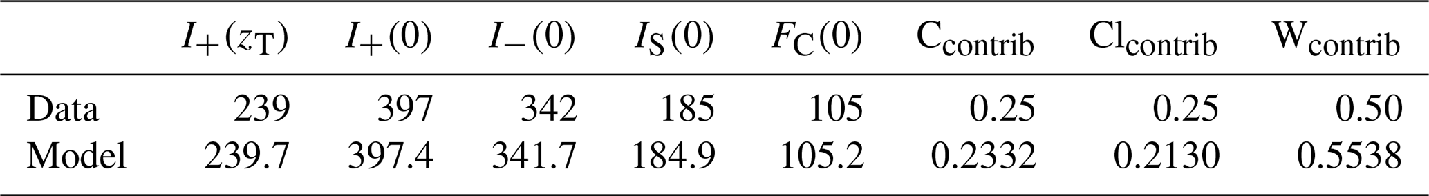
Using these parameter settings, we minimized the sum of squares of the differences between the data from Table B3 (after nondimensionalization) with the model outputs allowing the parameters k_S, k_C, k_W, k_Cl, b, and C_D to vary. In the minimization calculation, the terms associated with the contribution values (last three columns of Table B3) were given a heuristic weight of 0.01, since these values are less reliable than the other data. The resulting calibrated values for these parameters are given in Table B2; the results of the fitting are given in Table B3 and Fig. B1. As can be seen in Table B3, the minimization achieved very good agreement with the globally averaged data.

Figure B1 Model calibrated to global average values. The vertical axis in all the plots is the pressure. (a) Energy transport via radiative terms, and latent and sensible heat. (b) Atmospheric temperature. The red asterisk marks the surface temperature, T_S. (c) Atmospheric heat transport, F_A. (d) Vertical wind speed. (e) Density.

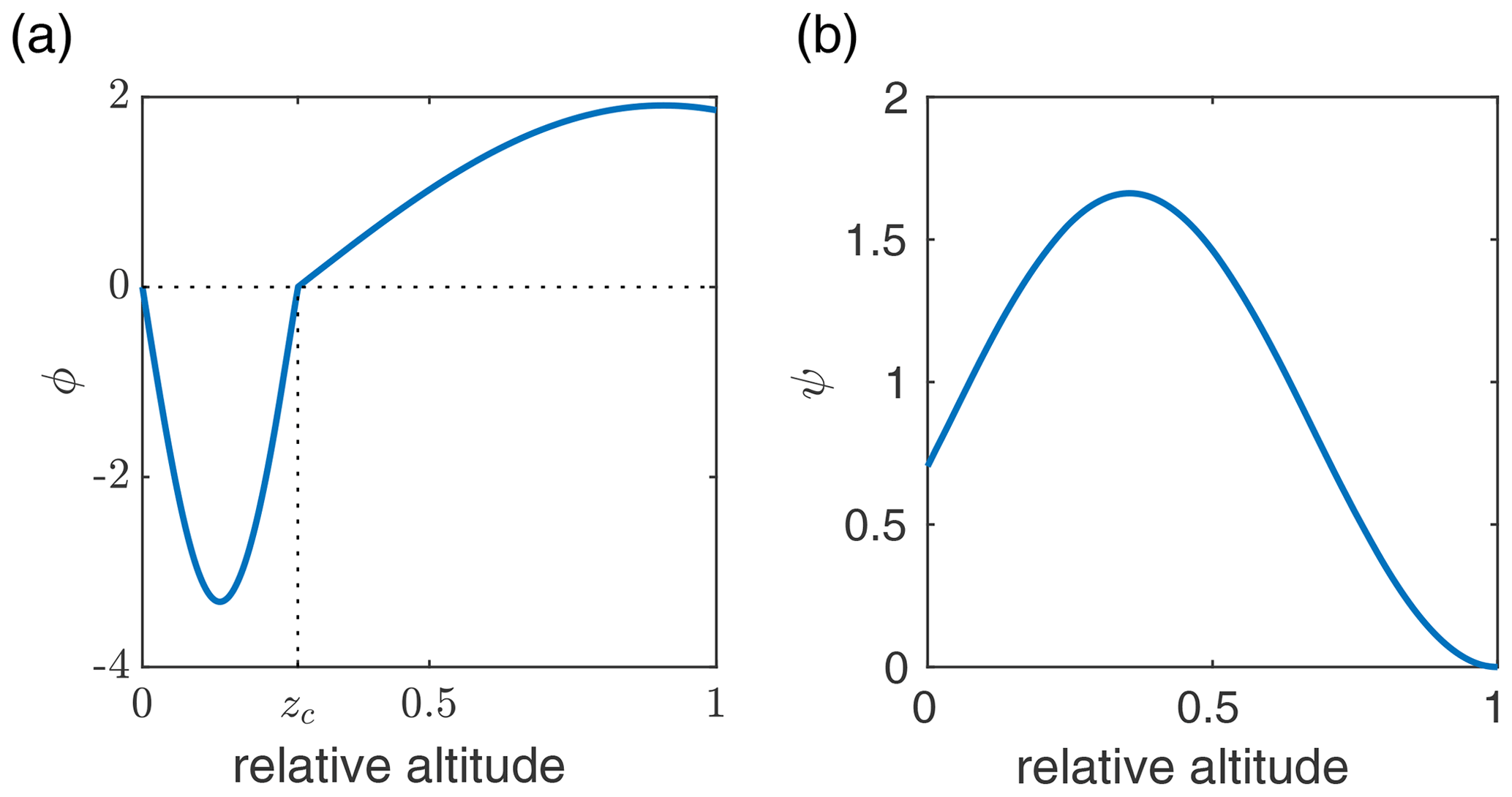
Using the calibrated values for k_S, k_C, k_W, k_Cl, b, and C_D obtained from the first step, the second calibration step was to select the parameters for the functions $\mathit{\varphi }\left(\widehat{z}\right)$ and $\mathit{\psi }\left(\widehat{z}\right)$ to attempt to match the annual temperature profile for the Arctic from Cronin and Jansen (2016, Fig. 1). Data from that figure of their paper are reproduced in Table B4. The Arctic values of the geographic-dependent parameters from Table B2 were used. Using each of the four forms for ϕ, given by Eqs. (A55)–(A58), and each of the two forms for F_A, given by Eqs. (A52) and (A53), the sum of the square of the differences between the model and the data in Table B4 was minimized by allowing the parameters z_c, Φ_B, L_ϕT, L_ϕB, and L_ψ to vary. The fit quality is shown in Fig. B2. From this figure it is evident that the first two forms for ϕ, namely Eqs. (A55) and (A56), do not give adequate fits. The other two forms for ϕ are similar, and both forms of ψ only give small changes. The best fit is the third form for ϕ and the second form for ψ, that is, Eqs. (A57) and (A53), and so these forms were chosen for the model. The calibrated parameters for these forms of ϕ and ψ are given in Table B2, and the corresponding functions ϕ and ψ are shown in Fig. B3.

Table B4 Annual Arctic temperature data from Fig. 1 of Cronin and Jansen (2016).

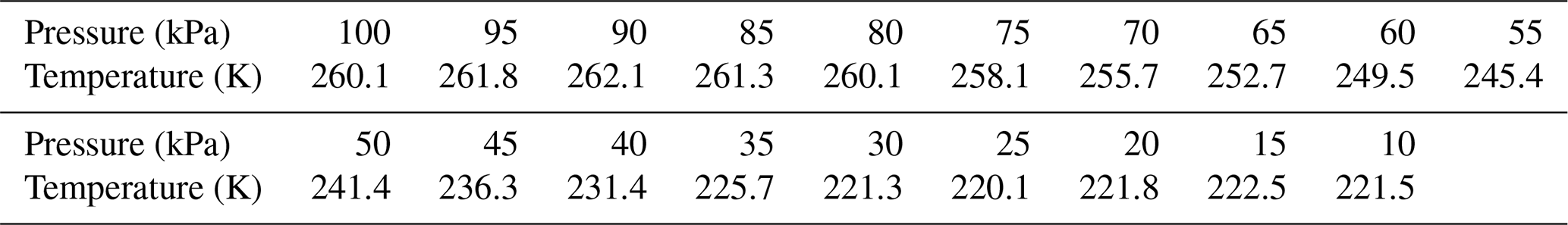
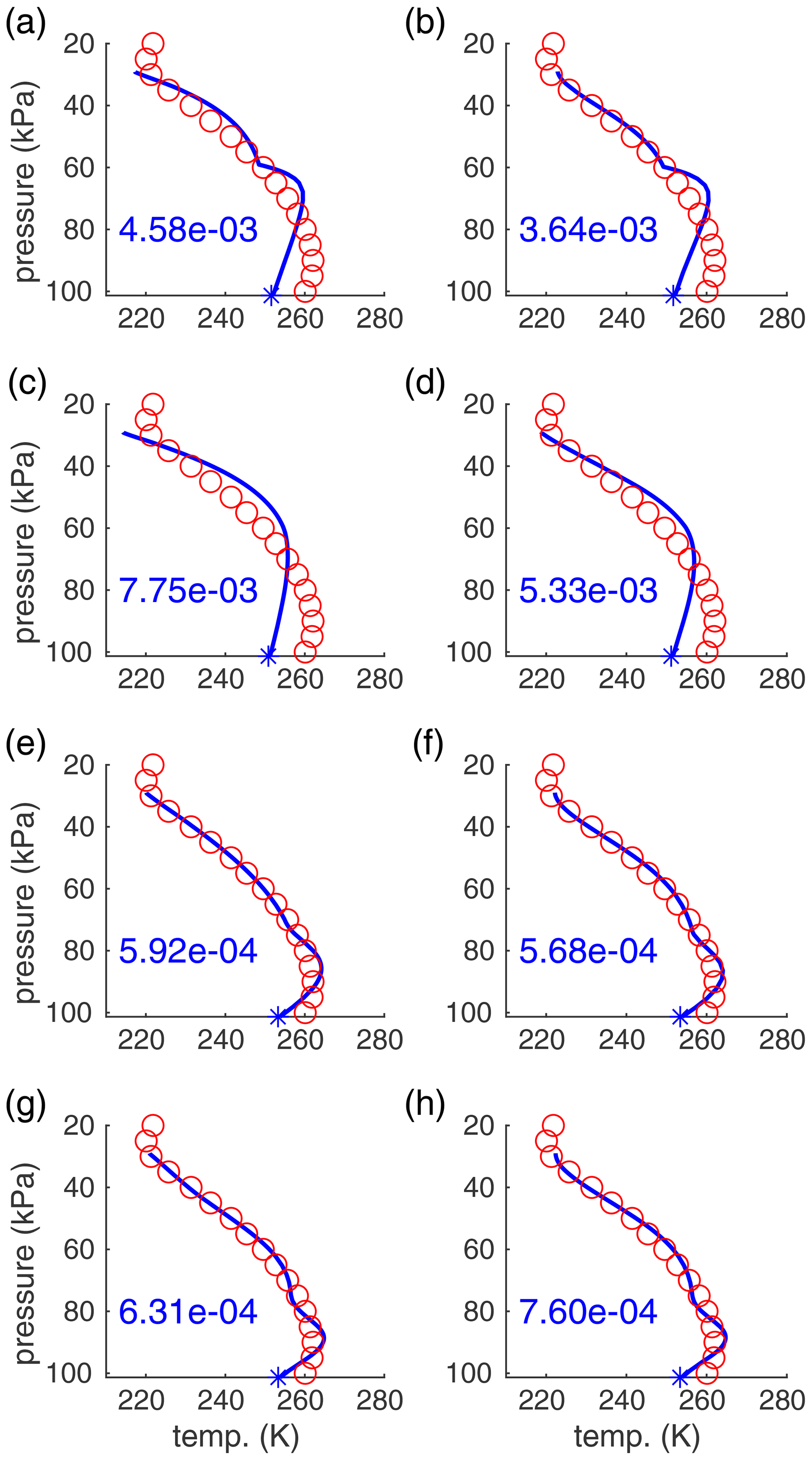
Figure B2 Temperature profiles for best fits for each of the forms of ϕ and ψ. Panels (a) and (b) correspond to Eq. (A55) for ϕ and panels (c) and (d) to Eq. (A56), and similarly, panels (e–h) correspond to Eqs. (A57) and (A58), respectively. Panels (a), (c), (e), and (g) correspond to Eq. (A52) for ψ, while panels (b), (d), (f), and (h) correspond to Eq. (A53). The data from Cronin and Jansen (2016) are the red circles. The numbers in the bottom left are the residuals for the fits.

Figure B3 Calibrated functions: (a) ϕ and (b) ψ.

For the above calibrations, the albedo values α_c and α_w in Eq. (A23) were set to the same constant value ($\mathrm{24}/\mathrm{185}$ for calibration to global data, $\mathrm{2}/\mathrm{3}$ for calibration to Arctic data) in order to ensure the empirical albedo value was matched regardless of the surface temperature. Now that the calibrations are complete, we wish to apply the model to the Arctic using different values of the carbon dioxide level. As such, we must choose values of α_c, α_w, and ω that allow for the albedo to change appropriately with surface temperature. The empirical albedo of $\mathrm{2}/\mathrm{3}$, which was used in the Arctic calibration, resulted in a surface temperature of T_S=253.4 K. Since this temperature is well below freezing, the albedo at this temperature should be near the maximum albedo, so α_c was set to 0.667. Second, α_w was set to 0.1, corresponding to the fact that, north of 70^∘ latitude, the Earth is mostly ocean-covered (albedo 0.06 for open water) and partly land (albedo 0.1–0.4). The value of ω was then calculated from Eq. (16) so that $\mathit{\alpha }\left(\mathrm{253.4}\right)=\mathrm{2}/\mathrm{3}$. This resulted in ω=0.01942.

B2 Insolation

This section presents the calculation of the insolation used in the Arctic model, where, in particular, the insolation is taken as an annual average over the region north of 70^∘ N.

Select a Cartesian coordinate system $(x,y,z)$ for the solar system with the Sun at the origin, with the z axis perpendicular to the Earth's orbital plane and with the positive x axis defined by the direction in the orbital plane from the Sun to the centre of the Earth when the Earth's North Pole is furthest from the Sun (Northern Hemisphere winter solstice). Let (r,θ) be the usual polar coordinates for the centre of the Earth on the orbital plane. Approximate the incoming solar radiation to the Earth as parallel rays travelling from the direction $q=-[\cos \mathit{\theta },\sin \mathit{\theta },\mathrm{0}{]}^T$ with energy flux S₀=1366 W m⁻² (the solar constant). Let ϕ and ψ be the latitude and “longitude” of a location on the Earth's surface, where we assume that ψ=0 is aligned with the positive x axis of the solar coordinate system, not with some fixed location on the Earth's surface. If the Earth's axis of rotation was parallel to the z axis (no tilt), then the unit outward normal to the Earth's surface in the solar coordinate system would be

$$\left[\begin{array}{c}\cos \mathit{\varphi }\cos \mathit{\psi }\\ \cos \mathit{\varphi }\sin \mathit{\psi }\\ \sin \mathit{\varphi }\end{array}\right],-{\displaystyle \frac{\mathit{\pi }}{\mathrm{2}}}\le \mathit{\varphi }\le {\displaystyle \frac{\mathit{\pi }}{\mathrm{2}}},-\mathit{\pi }<\mathit{\psi }\le \mathit{\pi }.$$

However, the Earth's axis is actually tilted by an angle $\mathit{\beta }=(\mathrm{23.5}/\mathrm{180})\mathit{\pi }$ in the negative sense in the (x,z) plane. Applying this tilt gives the unit outward normal as

$$\begin{array}{ll}{\displaystyle }n& {\displaystyle }=\left[\begin{array}{ccc}\cos \mathit{\beta }& \mathrm{0}& \sin \mathit{\beta }\\ \mathrm{0}& \mathrm{1}& \mathrm{0}\\ -\sin \mathit{\beta }& \mathrm{0}& \cos \mathit{\beta }\end{array}\right]\left[\begin{array}{c}\cos \mathit{\varphi }\cos \mathit{\psi }\\ \cos \mathit{\varphi }\sin \mathit{\psi }\\ \sin \mathit{\varphi }\end{array}\right]\\ {\displaystyle }& {\displaystyle }=\left[\begin{array}{c}\cos \mathit{\beta }\cos \mathit{\varphi }\cos \mathit{\psi }+\sin \mathit{\beta }\sin \mathit{\varphi }\\ \cos \mathit{\varphi }\sin \mathit{\psi }\\ -\sin \mathit{\beta }\cos \mathit{\varphi }\cos \mathit{\psi }+\cos \mathit{\beta }\sin \mathit{\varphi }\end{array}\right].\end{array}$$

The insolation striking the Earth's surface at (ϕ,ψ) is then $S_{\mathrm{0}}max(q\cdot n,\mathrm{0})$, where the maximum is due to the fact that the dot product is negative for points on the dark side of the Earth, away from the Sun, and hence the insolation there is zero.

Let S be the region of the Earth between latitudes ϕ₁ and ϕ₂. The area element is dS=R²cos ϕdψdϕ, where R is the radius of the Earth. Therefore the average annual (θ runs 0 to 2π) insolation in a region, S, of the Earth is

$$\begin{array}{ll}{\displaystyle }Q=& {\displaystyle }{\displaystyle \frac{{\int }_{\mathrm{0}}^{\mathrm{2}\mathit{\pi }}{\int }_S{S}_{\mathrm{0}}max(q\cdot n,\mathrm{0})\mathrm{d}S\mathrm{d}\mathit{\theta }}{{\int }_S\mathrm{d}S}}\\ {\displaystyle }=& {\displaystyle }{\displaystyle \frac{S_{\mathrm{0}}}{\mathrm{2}\mathit{\pi }\left(\sin {\mathit{\varphi }}_{\mathrm{2}}-\sin {\mathit{\varphi }}_{\mathrm{1}}\right)}}\\ {\displaystyle }& {\displaystyle }\times \underset{\mathrm{0}}{\overset{\mathrm{2}\mathit{\pi }}{\int }}\underset{{\mathit{\varphi }}_{\mathrm{1}}}{\overset{{\mathit{\varphi }}_{\mathrm{2}}}{\int }}\underset{-\mathit{\pi }}{\overset{\mathit{\pi }}{\int }}max(q\cdot n,\mathrm{0})\cos \mathit{\varphi }\mathrm{d}\mathit{\psi }\mathrm{d}\mathit{\varphi }\mathrm{d}\mathit{\theta }.\end{array}$$

Numerical integration of the above formula yields Q=341 W m⁻² for the entire globe, which agrees well with Wild's value of 340 (the difference is likely due to some ambiguity in the precise value of S₀), and yields Q=185 W m⁻² for the Arctic region north of 70^∘ latitude. If one considers the limit as the region of interest shrinks to size zero around the North Pole, the value of the insolation approaches the limit 173.85 W m⁻².