Effects of rotation and topography on internal solitary waves governed by the rotating Gardner equation

Nonlinear oceanic internal solitary waves are considered under the influence of the combined effects of saturating nonlinearity, Earth's rotation, and horizontal depth inhomogeneity. Here the basic model is the extended Korteweg–de Vries equation that includes both quadratic and cubic nonlinearity (the Gardner equation) with additional terms incorporating slowly varying depth and weak rotation. The complicated interplay between these different factors is explored using an approximate adiabatic approach and then through numerical solutions of the governing variable depth, i.e., the rotating Gardner model. These results are also compared to analysis in the Korteweg–de Vries limit to highlight the effect of the cubic nonlinearity. The study explores several particular cases considered in the literature that included some of these factors to illustrate limitations. Solutions are made to illustrate the relevance of this extended Gardner model for realistic oceanic conditions.

1 Introduction

Oceanic internal waves are an important class of nonlinear wave processes. In particular, the internal solitary waves (ISWs) are the most ubiquitous type of solitons in the natural environment. These waves often propagate for long distances over several inertial periods, and the effect of Earth's background rotation is potentially significant (e.g., Farmer et al., 2009; Grimshaw et al., 2014; Helfrich, 2007; Ostrovsky and Helfrich, 2019). The large ISWs in the South China Sea are prominent examples (Zhao and Alford, 2006; Alford et al., 2010). There are also numerous remote sensing images throughout the coastal oceans that show multiple wave packets (e.g., Jackson, 2004), indicating that the ISWs persist over periods longer than the local inertial period. It is also known that rotation destroys internal solitons due to resonant radiation of inertia–gravity waves (terminal damping; see Grimshaw et al., 1998a). The theoretical modeling of such processes often uses the rotation-modified Korteweg–de Vries equation (rKdV) derived for nonlinear waves in rotating ocean (Ostrovsky, 1978). In application to the oceanic conditions, this equation may need additional modifications, specifically for the variable depth along the propagation path. This specific case was considered in Grimshaw et al. (2014), Ostrovsky and Helfrich (2019), and Stepanyants (2019).

The rotation-induced solitary wave decay can be suppressed in certain ambient shear flows wherein the sign of the rotation coefficient is changed (Alias et al., 2014). In those cases, the rKdV equation supports solitary wave solutions. This interesting situation is not considered in this paper.

Another important feature of oceanic solitons is that, in many cases, they are strongly nonlinear, so that the Korteweg–de Vries approximation (KdV) involving only the quadratic nonlinearity is inapplicable (e.g., Apel et al., 2007; Helfrich and Grimshaw, 2008; Ostrovsky and Grue, 2003; Ostrovsky and Irisov, 2017). A better approximation of the real processes can be given by the Gardner equation that extends KdV by adding a cubic nonlinear amplitude term. It is significant when the quadratic and cubic nonlinear terms are of a comparable small amplitude. In that situation, higher-order corrections for dispersion and nonlinear dispersive terms are negligible. For example, this is the case in a two-layer fluid when the layer depths are nearly equal. Gardner solutions preserve the qualitative features of strongly nonlinear waves, such as the existence of a limiting soliton amplitude at which its length infinitely increases, whereas a KdV soliton amplitude can increase unlimitedly, with its width tending to zero. Moreover, in many cases, the Gardner equation gives a good quantitative approximation for strong solitons beyond the formal limits of its applicability (Stanton and Ostrovsky, 1998; Pelinovsky et al., 2000; Grimshaw et al., 2004) and thus has become the phenomenological model of choice. There are numerous studies using the Gardner equation in applications to oceanic waves, including its extension for the rotating ocean (e.g., Holloway et al., 1999; Obregon et al., 2018; Talipova et al., 2015).

In this paper, we make the next step by adding a sloping bottom effect to the Gardner model with rotation. Correspondingly, the results of Grimshaw et al. (2014), Ostrovsky and Helfrich (2019), and Stepanyants (2019) can be significantly modified. In particular, we discuss an interplay between the effects of nonlinearity, rotation, and inhomogeneity. Some realistic estimates are also given.

The work by Karczewska and Rozmej (2020) considers the analogs of the KdV and Boussinesq equations for shallow water waves with different relative orders of the following small perturbing factors: nonlinearity, dispersion, and bottom slope. Then various terms, such as nonlinear dispersive terms, can prevail over other perturbations. Here we consider a certain (although rather general) physical problem when all included terms are of the same order and the classical description is sufficient.

2 Rotating Gardner equation

A standard model for the evolution of large-amplitude oceanic internal solitary waves is the rotating Gardner (rG), or extended KdV equation with rotation and variable depth h(x) (Holloway et al., 1999), as follows:

$$\begin{array}{}\text{(1)}& {\displaystyle \frac{\partial }{\partial x}}\left[{\displaystyle \frac{\partial \mathit{\eta }}{\partial t}}+\left(c+\mathit{\alpha }\mathit{\eta }+\mathit{\nu }{\mathit{\eta }}^{\mathrm{2}}\right){\displaystyle \frac{\partial \mathit{\eta }}{\partial x}}+\mathit{\beta }{\displaystyle \frac{{\partial }^{\mathrm{3}}\mathit{\eta }}{\partial x^{\mathrm{3}}}}+{\displaystyle \frac{c}{\mathrm{2}}}{\displaystyle \frac{Q_x}{Q}}\mathit{\eta }\right]=\mathit{\gamma }\mathit{\eta }.\end{array}$$

Here the wave amplitude function η(x,t) depends on the horizontal position x and time t. The linear long wave phase speed c is found from an eigenvalue problem for the structure function Φ(z) of a specified vertical mode. Both c and Φ(z) are slow functions of x. The x-dependent coefficients α, ν, β, Q, and γ of the quadratic nonlinear, cubic nonlinear, non-hydrostatic, inhomogeneous, and rotation terms, respectively, are found as integrals over the depth of Φ or Φ^′ and the background stratification $\stackrel{\mathrm{‾}}{\mathit{\rho }}\left(z\right)$ and current $\stackrel{\mathrm{‾}}{u}\left(z\right)$. They can be found in numerous publications (e.g., Holloway et al., 1999; Grimshaw et al., 2004) and are summarized briefly in Appendix A. When considering a spatially inhomogeneous situation, it is advantageous to switch from the (x,t) system to the (s,x) system, where

$$\begin{array}{}\text{(2)}& s=\underset{\mathrm{0}}{\overset{x}{\int }}{\displaystyle \frac{\mathrm{d}x}{c}}-t.\end{array}$$

If, additionally, $\mathit{\zeta }=Q^{\mathrm{1}/\mathrm{2}}\mathit{\eta }$ is introduced, then Eq. (1) becomes the following:

$$\begin{array}{}\text{(3)}& {\displaystyle \frac{\partial }{\partial s}}\left[{\displaystyle \frac{\partial \mathit{\zeta }}{\partial x}}+{\displaystyle \frac{\mathit{\alpha }}{c^{\mathrm{2}}{Q}^{\mathrm{1}/\mathrm{2}}}}\mathit{\zeta }{\displaystyle \frac{\partial \mathit{\zeta }}{\partial s}}+{\displaystyle \frac{\mathit{\nu }}{c^{\mathrm{2}}Q}}{\mathit{\zeta }}^{\mathrm{2}}{\displaystyle \frac{\partial \mathit{\zeta }}{\partial s}}+{\displaystyle \frac{\mathit{\beta }}{c^{\mathrm{4}}}}{\displaystyle \frac{{\partial }^{\mathrm{3}}\mathit{\zeta }}{\partial s^{\mathrm{3}}}}\right]=\mathit{\gamma }\mathit{\zeta }.\end{array}$$

We note that here ζ²=Qη² is the wave action flux. Equation (3) can be shown to have two conserved quantities, as follows:

$$\begin{array}{}\text{(4)}& M=\int \mathit{\zeta }\mathrm{d}s\mathrm{and}E=\int {\mathit{\zeta }}^{\mathrm{2}}\mathrm{d}s,\end{array}$$

where the integrals are over the full s domain (infinite or periodic). These are, respectively, mass- and energy-related quantities, as discussed further in the next section.

Additionally, any initial condition to Eq. (3) with γ≠0 must satisfy the zero mass requirement, as follows (Ostrovsky, 1978):

$$\begin{array}{}\text{(5)}& \underset{T/\mathrm{2}}{\overset{-T/\mathrm{2}}{\int }}\mathit{\zeta }(s,\mathrm{0})\mathrm{d}s=\mathrm{0},\end{array}$$

where $s=-t$ at x=0, and T is the length of the time domain.

In the absence of rotation, γ=0, Eq. (3) reduces to the Gardner equation. This permits the solitary wave solution, as follows:

$$\begin{array}{}\text{(6)}& \mathit{\zeta }={\displaystyle \frac{a}{\mathrm{1}+B\cosh \left[\mathit{\sigma }\right(s-\mathit{\kappa }x\left)\right]}},\end{array}$$

which is described by the parameter B. Here,

$$\begin{array}{}\text{(7)}& a={\displaystyle \frac{Q^{\mathrm{1}/\mathrm{2}}\mathit{\alpha }}{\mathit{\nu }}}(B^{\mathrm{2}}-\mathrm{1}),{\mathit{\sigma }}^{\mathrm{2}}={\displaystyle \frac{c^{\mathrm{2}}\mathit{\alpha }a}{\mathrm{6}\mathit{\beta }{Q}^{\mathrm{1}/\mathrm{2}}}},\mathit{\kappa }={\displaystyle \frac{\mathit{\beta }{\mathit{\sigma }}^{\mathrm{2}}}{c^{\mathrm{4}}}}.\end{array}$$

The amplitude, A, in terms of η ($=\mathit{\zeta }{Q}^{-\mathrm{1}/\mathrm{2}}$) is as follows:

$$\begin{array}{}\text{(8)}& A={\displaystyle \frac{a{Q}^{-\mathrm{1}/\mathrm{2}}}{\mathrm{1}+B}}={\displaystyle \frac{\mathit{\alpha }}{\mathit{\nu }}}(B-\mathrm{1}).\end{array}$$

From the mass constraint (Eq. 5), a solitary wave initial condition requires the addition of a constant pedestal, as follows:

$$d=-{\displaystyle \frac{\mathrm{1}}{T}}\underset{T/\mathrm{2}}{\overset{-T/\mathrm{2}}{\int }}\mathit{\zeta }(s,\mathrm{0})\mathrm{d}s,$$

with ζ given by Eq. (6).

There are three families of steady solitary wave solutions given by Eqs. (6)–(8) (Grimshaw et al., 1999). When ν<0, solitary wave solutions require $\mathrm{0}<B<\mathrm{1}$ and have polarity αA>0. They approach the sech² KdV solitary wave as B→1, and as B→0, the solution approaches the maximum amplitude, $A_{\max }=-\mathit{\alpha }/\mathit{\nu }$, or flat-top wave. When ν>0, solitary wave solutions require B²>1, and there are two solution branches. For B>1, αA>0, and there is no limit on the wave amplitude. The sech² KdV wave is recovered as B→1 from above, and for B≫1, the solution approaches the sech solution of the modified KdV equation (i.e., the Gardner equation with α=0). The third branch occurs for $B<-\mathrm{1}$ with the wave polarity αA<0. In this case, solitary wave amplitude has a minimum amplitude $A_{\min }=-\mathrm{2}\mathit{\alpha }/\mathit{\nu }$ obtained as $B\to -\mathrm{1}$ from below. This limiting wave has an algebraic structure, and for $B\ll -\mathrm{1}$, the solution again approaches the sech wave of modified KdV equation. For ν>0, there are also localized pulsating traveling wave solutions (breathers) that have a total negative mass between zero and the mass of the limiting solitary wave at $B=-\mathrm{1}$ (Pelinovsky and Grimshaw, 1997).

3 Adiabatic evolution of solitary waves

Assuming that ζ→0 for $\left|s\right|\to \mathrm{\infty }$, and integrating Eq. (3), gives the following:

$$\begin{array}{}\text{(9)}& {\displaystyle \frac{\partial \mathit{\zeta }}{\partial x}}+{\displaystyle \frac{\mathit{\alpha }}{c^{\mathrm{2}}{Q}^{\mathrm{1}/\mathrm{2}}}}\mathit{\zeta }{\displaystyle \frac{\partial \mathit{\zeta }}{\partial s}}+{\displaystyle \frac{\mathit{\nu }}{c^{\mathrm{2}}Q}}{\mathit{\zeta }}^{\mathrm{2}}{\displaystyle \frac{\partial \mathit{\zeta }}{\partial s}}+{\displaystyle \frac{\mathit{\beta }}{c^{\mathrm{4}}}}{\displaystyle \frac{{\partial }^{\mathrm{3}}\mathit{\zeta }}{\partial s^{\mathrm{3}}}}=-\mathit{\gamma }\underset{s}{\overset{\mathrm{\infty }}{\int }}\mathit{\zeta }\mathrm{d}{s}^{\prime }.\end{array}$$

Multiplication by ζ and integration in s from −∞ to ∞ gives the following:

$$\begin{array}{}\text{(10)}& {\displaystyle \frac{d}{\mathrm{d}x}}\left(\underset{-\mathrm{\infty }}{\overset{\mathrm{\infty }}{\int }}{\mathit{\zeta }}^{\mathrm{2}}\mathrm{d}s\right)=-\mathrm{2}\mathit{\gamma }\underset{-\mathrm{\infty }}{\overset{\mathrm{\infty }}{\int }}\left(\underset{s}{\overset{\mathrm{\infty }}{\int }}\mathit{\zeta }\mathrm{d}{s}^{\prime }\right)\mathrm{d}s=-\mathit{\gamma }{\left(\underset{-\mathrm{\infty }}{\overset{\mathrm{\infty }}{\int }}\mathit{\zeta }\mathrm{d}s\right)}^{\mathrm{2}}.\end{array}$$

The solution of the rG equation (Eq. 9) implies that the right side of Eq. (10) is zero and E is a constant. However, progress can be made if we start with a solitary wave from Eq. (6), assume that the inhomogeneous and rotational effects are very weak, such that the evolving wave remains a solitary wave but with slowly varying amplitude, and take the limits of integration to contain only the evolving solitary wave. With the solitary wave solution (Eq. 6) written as follows:

$$\begin{array}{}\text{(11)}& \mathit{\zeta }=a\mathcal{F}\left(y\right),\mathcal{F}={\displaystyle \frac{\mathrm{1}}{\mathrm{1}+B\cosh \left(y\right)}},\mathrm{and}y=\mathit{\sigma }s.\end{array}$$

Equation (9) gives the following:

$$\begin{array}{}\text{(12)}& {\displaystyle \frac{d}{\mathrm{d}x}}\left({\displaystyle \frac{a^{\mathrm{2}}}{\mathit{\sigma }}}{\mathcal{I}}_{\mathrm{2}}\right)=-\mathit{\gamma }{\displaystyle \frac{a^{\mathrm{2}}}{{\mathit{\sigma }}^{\mathrm{2}}}}{\mathcal{I}}_{\mathrm{1}}^{\mathrm{2}},\end{array}$$

where

$$\begin{array}{}\text{(13)}& {\mathcal{I}}_n=\underset{-\mathrm{\infty }}{\overset{\mathrm{\infty }}{\int }}{\mathcal{F}}^n\mathrm{d}y,n=\mathrm{1},\mathrm{2}.\end{array}$$

The result, Eq. (12), is a statement for the variation in the energy,

$$\begin{array}{}\text{(14)}& E_{\mathrm{w}}={\displaystyle \frac{a^{\mathrm{2}}}{\mathit{\sigma }}}{\mathcal{I}}_{\mathrm{2}},\end{array}$$

of the slowly evolving solitary wave. In the absence of rotation, E_w is conserved; however, the wave mass,

$$\begin{array}{}\text{(15)}& M_{\mathrm{w}}={\displaystyle \frac{a}{\mathit{\sigma }}}{\mathcal{I}}_{\mathrm{1}},\end{array}$$

is not necessarily conserved. Changes in M_w are compensated by the formation of a trailing shelf. For example, in the typical case with ν<0 of a solitary wave approaching a point of polarity reversal, α=0, the wave mass increases in magnitude (Grimshaw et al., 1998b). Thus, the trailing shelf must have the sign opposite to the wave polarity. When ν>0, the situation is more subtle, but again, any variations in M_w are compensated by a shelf (Grimshaw et al., 1999; Nakoulima et al., 2004). In a homogeneous rotating environment, both E_w and M_w decrease with x and are compensated by the trailing wave radiation (Grimshaw et al., 1998a). With both inhomogeneity and rotation, the energy will decrease with x, but the wave mass may increase or decrease, depending on the interplay between these two effects.

In the KdV equation, ρ₀E_w is the solitary wave energy, ∬pu dzdt. Here p and u are the first-order, wave-induced pressure and horizontal velocity fields. With the addition of the cubic nonlinear term in the Gardner equation, E_w is not exactly the wave energy but is still a good measure of it. The actual wave mass is $Q^{-\mathrm{1}/\mathrm{2}}{M}_w$, with Q defined as in Eq. (A3d).

3.1 Rotating KdV equation

For later reference, we first consider the adiabatic theory for the rotating KdV equation (ν=0) from Grimshaw et al. (2014). The solitary wave solution is found from Eqs. (6) and (8), with B=1 as follows:

$$\begin{array}{}\text{(16)}& \mathit{\zeta }=a\mathcal{F},\mathcal{F}={\mathrm{sech}}^{\mathrm{2}}\left(y\right),{\mathit{\sigma }}^{\mathrm{2}}={\displaystyle \frac{c^{\mathrm{2}}\mathit{\alpha }a}{\mathrm{12}\mathit{\beta }{Q}^{\mathrm{1}/\mathrm{2}}}},a=A{Q}^{\mathrm{1}/\mathrm{2}}.\end{array}$$

From Eq. (13), ℐ₁=2 and ${\mathcal{I}}_{\mathrm{2}}=\mathrm{4}/\mathrm{3}$, and Eq. (12) gives the following:

$$\begin{array}{}\text{(17)}& {\displaystyle \frac{d}{\mathrm{d}x}}\left({\displaystyle \frac{\mathrm{4}}{\mathrm{3}}}{\displaystyle \frac{a^{\mathrm{2}}}{\mathit{\sigma }}}\right)=-\mathrm{4}\mathit{\gamma }{\displaystyle \frac{a^{\mathrm{2}}}{{\mathit{\sigma }}^{\mathrm{2}}}}.\end{array}$$

This can be written as follows:

$${\displaystyle \frac{d}{\mathrm{d}x}}{\mathcal{A}}^{\mathrm{3}/\mathrm{2}}=-\mathrm{3}\mathit{\gamma }{w}^{\mathrm{2}}\mathcal{A},\mathcal{A}=wa,w={\left({\displaystyle \frac{\mathrm{12}\mathit{\beta }{Q}^{\mathrm{1}/\mathrm{2}}}{\mathit{\alpha }{c}^{\mathrm{2}}}}\right)}^{\mathrm{1}/\mathrm{3}}.$$

When integrated, this gives the following:

$$\begin{array}{}\text{(18)}& \begin{array}{rl}{\displaystyle \frac{A}{A_{\mathrm{0}}}}& ={\left({\displaystyle \frac{Q_{\mathrm{0}}}{Q}}\right)}^{\mathrm{1}/\mathrm{2}}{\displaystyle \frac{a}{a_{\mathrm{0}}}}={\left({\displaystyle \frac{Q_{\mathrm{0}}}{Q}}\right)}^{\mathrm{1}/\mathrm{2}}{\displaystyle \frac{w_{\mathrm{0}}}{w}}\\ & {\left[\mathrm{1}-(w_{\mathrm{0}}{a}_{\mathrm{0}}{)}^{-\mathrm{1}/\mathrm{2}}\underset{\mathrm{0}}{\overset{x}{\int }}\mathit{\gamma }{w}^{\mathrm{2}}\mathrm{d}{x}^{\prime }\right]}^{\mathrm{2}}.\end{array}\end{array}$$

The 0 subscript indicates the initial value at x=0.

In the absence of rotation, γ=0, the conservation of wave action gives the following:

$$\begin{array}{}\text{(19)}& {\displaystyle \frac{A}{A_{\mathrm{0}}}}={\left({\displaystyle \frac{Q_{\mathrm{0}}}{Q}}\right)}^{\mathrm{1}/\mathrm{2}}{\displaystyle \frac{w_{\mathrm{0}}}{w}}={\left({\displaystyle \frac{Q_{\mathrm{0}}^{\mathrm{2}}{\mathit{\beta }}_{\mathrm{0}}}{{\mathit{\alpha }}_{\mathrm{0}}{c}_{\mathrm{0}}^{\mathrm{2}}}}{\displaystyle \frac{\mathit{\alpha }{c}^{\mathrm{2}}}{Q^{\mathrm{2}}\mathit{\beta }}}\right)}^{\mathrm{1}/\mathrm{3}}.\end{array}$$

For a homogeneous rotating environment, Eq. (18) gives the following:

$$\begin{array}{}\text{(20)}& {\displaystyle \frac{A}{A_{\mathrm{0}}}}={\left[\mathrm{1}-{\displaystyle \frac{x}{X_{\mathrm{eO}}}}\right]}^{\mathrm{2}},X_{\mathrm{eO}}={\displaystyle \frac{c}{\mathit{\gamma }}}{\left({\displaystyle \frac{\mathit{\alpha }{A}_{\mathrm{0}}}{\mathrm{12}\mathit{\beta }}}\right)}^{\mathrm{1}/\mathrm{2}}.\end{array}$$

The KdV solitary wave is completely extinguished by the radiation of the inertia–gravity waves in the finite distance X_eO.

3.2 Rotating Gardner equation

When ν≠0, the Gardner solitary wave solution (Eq. 11) and Eq. (13) give the following:

$$\begin{array}{}\text{(21)}& {\displaystyle }{\mathcal{I}}_{\mathrm{1}}={\displaystyle \frac{\mathrm{4}}{(B^{\mathrm{2}}-\mathrm{1}{)}^{\mathrm{1}/\mathrm{2}}}}\mathcal{T}\left(B\right),\text{(22)}& {\displaystyle }{\mathcal{I}}_{\mathrm{2}}={\displaystyle \frac{\mathrm{2}}{B^{\mathrm{2}}-\mathrm{1}}}-{\displaystyle \frac{\mathrm{4}}{(B^{\mathrm{2}}-\mathrm{1}{)}^{\mathrm{3}/\mathrm{2}}}}\mathcal{T}\left(B\right),\end{array}$$

where

$$\begin{array}{}\text{(23)}& \mathcal{T}\left(B\right)={\tan }^{-\mathrm{1}}\left({\displaystyle \frac{B-\mathrm{1}}{\sqrt{B^{\mathrm{2}}-\mathrm{1}}}}\right)=\mathrm{sgn}\left(B\right){\tan }^{-\mathrm{1}}\sqrt{{\displaystyle \frac{B-\mathrm{1}}{B+\mathrm{1}}}}.\end{array}$$

Substituting Eqs. (7), (21), and (22) into Eq. (12) gives the following:

$$\begin{array}{}\text{(24)}& \begin{array}{rl}{\displaystyle \frac{d}{\mathrm{d}x}}& \left[{\left({\displaystyle \frac{\mathrm{24}\mathit{\beta }{\mathit{\alpha }}^{\mathrm{2}}{Q}^{\mathrm{2}}}{c^{\mathrm{2}}{\mathit{\nu }}^{\mathrm{3}}}}\right)}^{\mathrm{1}/\mathrm{2}}\left[(B^{\mathrm{2}}-\mathrm{1}{)}^{\mathrm{1}/\mathrm{2}}-\mathrm{2}\mathcal{T}(B)\right]\right]\\ & =-\mathrm{96}{\displaystyle \frac{\mathit{\gamma }\mathit{\beta }Q}{c^{\mathrm{2}}\mathit{\nu }}}{\mathcal{T}}^{\mathrm{2}}\left(B\right).\end{array}\end{array}$$

This equation can be integrated to obtain B(x); hence A(x) is derived from Eq. (8). Since B→1 as ν→0, the equation remains regular for cases with ν(x) changing sign. Note also that it remains real for ν<0 and $\mathrm{0}<B<\mathrm{1}$, since ${\tan }^{-\mathrm{1}}\left(iy\right)=i{\tanh }^{-\mathrm{1}}\left(y\right)$.

Figure 1 $X_{\mathrm{eG}}/X_{\mathrm{eO}}$ as a function of B₀ for the three Gardner solitary wave regimes, with ν<0 for $\mathrm{0}<B_{\mathrm{0}}<\mathrm{1}$ and ν>0 for B²>1.

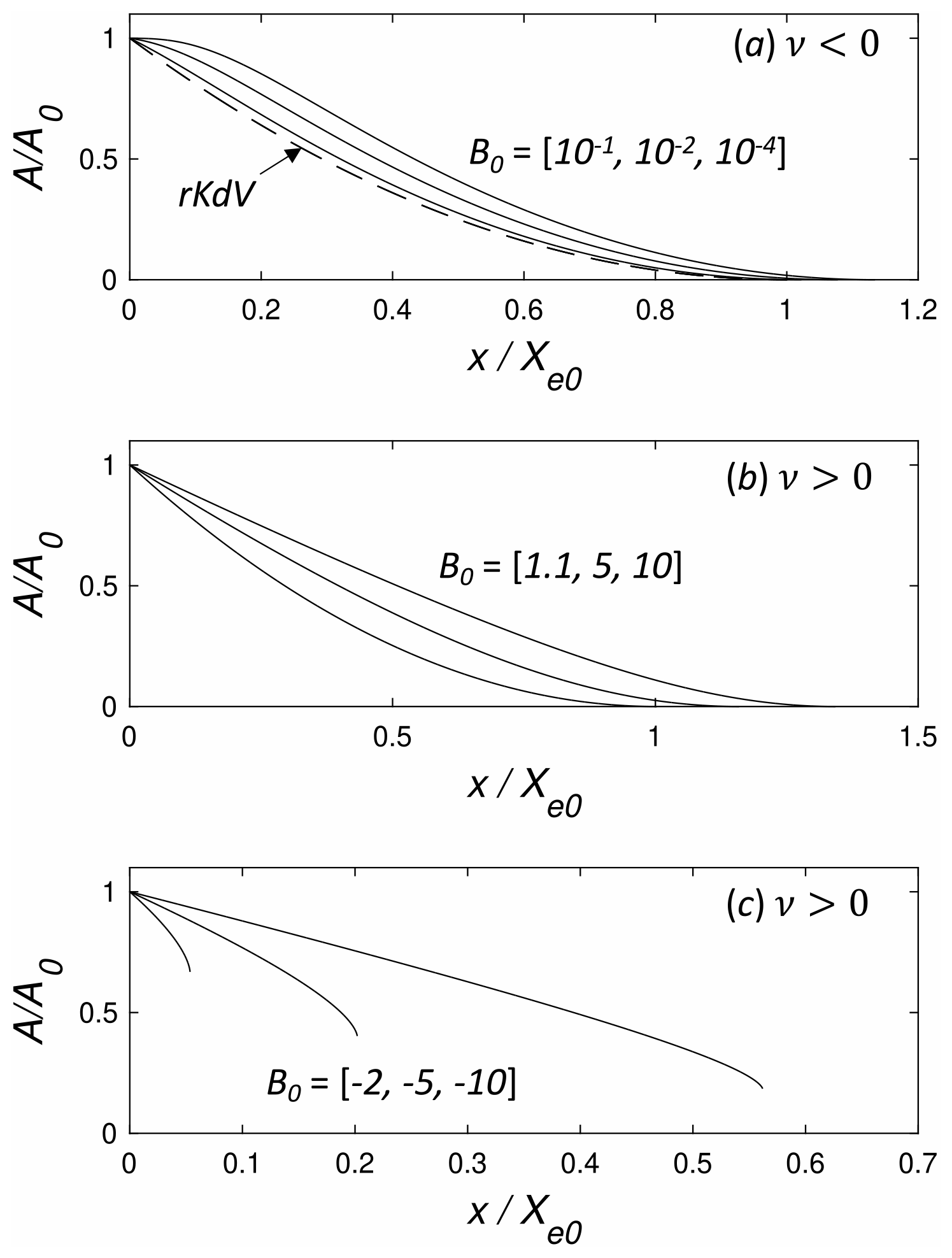
Figure 2 $A/A_{\mathrm{0}}$ versus $x/X_{\mathrm{eO}}$ for homogeneous conditions. (a) ν<0 for $B_{\mathrm{0}}=[{\mathrm{10}}^{-\mathrm{1}},{\mathrm{10}}^{-\mathrm{2}},{\mathrm{10}}^{-\mathrm{4}}]$ (solid lines from left to right). The dashed line is the rKdV equation solution (Eq. 20). (b) ν>0 and $B_{\mathrm{0}}=[\mathrm{1.1},\mathrm{5},\mathrm{10}]$ (from left to right). (c) ν>0 and $B_{\mathrm{0}}=[-\mathrm{2},-\mathrm{5},-\mathrm{10}]$ (from left to right).

Figure 3 Comparison of the rG adiabatic radiation decay theory for homogeneous conditions (black lines) and rG numerical solutions for (a) B₀=0.3, (b) $B_{\mathrm{0}}={\mathrm{10}}^{-\mathrm{4}}$, (c) B₀=5, and (d) $B_{\mathrm{0}}=-\mathrm{4}$. In panels (a) and (b), red (blue) indicates the numerical solutions of the rG equation (Eq. 30) for $\mathit{ϵ}=\mathrm{2.5}\times {\mathrm{10}}^{-\mathrm{5}}$ ($\mathrm{2.5}\times {\mathrm{10}}^{-\mathrm{3}}$). In panels (c) and (d), red (blue) indicates $\mathit{ϵ}=\mathrm{2.5}\times {\mathrm{10}}^{-\mathrm{3}}$ (0.25).

While it is not necessary to make the sign of ν explicit in integrating Eq. (24), for ν<0 ($\mathrm{0}<B<\mathrm{1}$), it can be written as follows:

$$\begin{array}{}\text{(25)}& \begin{array}{rl}{\displaystyle \frac{\sqrt{\mathrm{1}-B^{\mathrm{2}}}}{B}}& {\displaystyle \frac{\mathrm{d}B}{\mathrm{d}x}}={\displaystyle \frac{\mathrm{1}}{\mathrm{2}}}{\displaystyle \frac{d}{\mathrm{d}x}}\left[\ln \left({\displaystyle \frac{\mathit{\beta }{Q}^{\mathrm{2}}{\mathit{\alpha }}^{\mathrm{2}}}{c^{\mathrm{2}}|\mathit{\nu }{|}^{\mathrm{3}}}}\right)\right]\\ & \left(\mathrm{2}{\tanh }^{-\mathrm{1}}\sqrt{{\displaystyle \frac{\mathrm{1}-B}{\mathrm{1}+B}}}-\sqrt{\mathrm{1}-B^{\mathrm{2}}}\right)\\ & +\mathrm{8}\mathit{\gamma }{\left({\displaystyle \frac{\mathrm{6}\mathit{\beta }\left|\mathit{\nu }\right|}{c^{\mathrm{2}}{\mathit{\alpha }}^{\mathrm{2}}}}\right)}^{\mathrm{1}/\mathrm{2}}{\left({\tanh }^{-\mathrm{1}}\sqrt{{\displaystyle \frac{\mathrm{1}-B}{\mathrm{1}+B}}}\right)}^{\mathrm{2}}.\end{array}\end{array}$$

And for ν>0 (B²>1), it can be written as follows:

$$\begin{array}{}\text{(26)}& \begin{array}{rl}{\displaystyle \frac{\sqrt{B^{\mathrm{2}}-\mathrm{1}}}{B}}& {\displaystyle \frac{\mathrm{d}B}{\mathrm{d}x}}=-{\displaystyle \frac{\mathrm{1}}{\mathrm{2}}}{\displaystyle \frac{d}{\mathrm{d}x}}\left[\ln \left({\displaystyle \frac{\mathit{\beta }{Q}^{\mathrm{2}}{\mathit{\alpha }}^{\mathrm{2}}}{c^{\mathrm{2}}{\mathit{\nu }}^{\mathrm{3}}}}\right)\right]\\ & \left(\sqrt{B^{\mathrm{2}}-\mathrm{1}}-\mathrm{2}{\tan }^{-\mathrm{1}}\left({\displaystyle \frac{B-\mathrm{1}}{\sqrt{B^{\mathrm{2}}-\mathrm{1}}}}\right)\right)\\ & -\mathrm{8}\mathit{\gamma }{\left({\displaystyle \frac{\mathrm{6}\mathit{\beta }\mathit{\nu }}{c^{\mathrm{2}}{\mathit{\alpha }}^{\mathrm{2}}}}\right)}^{\mathrm{1}/\mathrm{2}}{\left[{\tan }^{-\mathrm{1}}\left({\displaystyle \frac{B-\mathrm{1}}{\sqrt{B^{\mathrm{2}}-\mathrm{1}}}}\right)\right]}^{\mathrm{2}}.\end{array}\end{array}$$

As discussed above, in a non-rotating system, the right-hand side of Eq. (24) is zero, and the conservation of wave energy gives the following:

$$\begin{array}{}\text{(27)}& E_{w\mathrm{0}}={\left({\displaystyle \frac{\mathrm{24}{Q}^{\mathrm{2}}{\mathit{\alpha }}^{\mathrm{2}}\mathit{\beta }}{c^{\mathrm{2}}{\mathit{\nu }}^{\mathrm{3}}}}\right)}^{\mathrm{1}/\mathrm{2}}\left[(B^{\mathrm{2}}-\mathrm{1}{)}^{\mathrm{1}/\mathrm{2}}-\mathrm{2}\mathcal{T}(B)\right],\end{array}$$

where E_w0 is a constant evaluated at x=0. This can be solved to give B(x).

Radiation decay in a homogeneous environments (where c, α, … are constants) was recently considered by Obregon et al. (2018). Here we briefly redevelop their decay result in our variables for clarity.

In a homogeneous environment, the first term on the right-hand side of Eq. (25) or Eq. (26) is zero. Then the distance, X_eG, to the complete radiation decay in the rG equation is found by the integration of Eq. (25) or Eq. (26), with the first term on the right side set to zero, from x=0 to X_eG, where B=B₀ and B_e, respectively. When A₀α>0, B₀>0, the solitary wave, decays from an initial amplitude $A_{\mathrm{0}}=\mathit{\alpha }{\mathit{\nu }}^{-\mathrm{1}}(B_{\mathrm{0}}-\mathrm{1})$ to zero when B_e=1, regardless of the sign of ν. While for ν>0 and A₀α<0, $B_{\mathrm{0}}<-\mathrm{1}$, and the solitary wave decay can be followed only to the limiting amplitude, $A_{\lim }=-\mathrm{2}\mathit{\alpha }/\mathit{\nu }$, where $B_{\mathrm{e}}=-\mathrm{1}$. These considerations give the following:

$$\begin{array}{}\text{(28)}& {\displaystyle \frac{X_{\mathrm{eG}}}{X_{\mathrm{eO}}}}={\displaystyle \frac{\sqrt{\mathrm{2}}}{\mathrm{8}}}\left\{\begin{array}{l}{\mathcal{I}}_B(B_{\mathrm{0}},\mathrm{1})|B_{\mathrm{0}}-\mathrm{1}{|}^{-\mathrm{1}/\mathrm{2}},B_{\mathrm{0}}>\mathrm{0},\\ {\mathcal{I}}_B(B_{\mathrm{0}},-\mathrm{1})(\mathrm{1}-B_{\mathrm{0}}{)}^{-\mathrm{1}/\mathrm{2}},B_{\mathrm{0}}<-\mathrm{1},\end{array}\right.\end{array}$$

where

$$\begin{array}{}\text{(29)}& {\mathcal{I}}_B(B_{\mathrm{0}},B_{\mathrm{e}})=\left\{\begin{array}{l}\underset{B_{\mathrm{0}}}{\overset{B_{\mathrm{e}}}{\int }}\frac{\sqrt{\mathrm{1}-B^{\mathrm{2}}}}{B}{\left({\tanh }^{-\mathrm{1}}\sqrt{\frac{\mathrm{1}-B}{\mathrm{1}+B}}\right)}^{-\mathrm{2}}dB,\mathit{\nu }<\mathrm{0},\\ -\underset{B_{\mathrm{0}}}{\overset{B_{\mathrm{e}}}{\int }}\frac{\sqrt{B^{\mathrm{2}}-\mathrm{1}}}{B}{\left({\tan }^{-\mathrm{1}}\sqrt{\frac{B-\mathrm{1}}{B+\mathrm{1}}}\right)}^{-\mathrm{2}}\mathrm{d}B,\mathit{\nu }>\mathrm{0}.\end{array}\right.\end{array}$$

Again, X_eO is the rKdV equation decay length (Eq. 20) evaluated using $\left|A_{\mathrm{0}}\mathit{\alpha }\right|$ when $B_{\mathrm{0}}<-\mathrm{1}$.

Figure 1 shows $X_{\mathrm{eG}}/X_{\mathrm{eO}}$ versus B₀ for all three wave regimes. For ν<0, where $\mathrm{0}<B_{\mathrm{0}}<\mathrm{1}$, $X_{\mathrm{eG}}/X_{\mathrm{eO}}\approx \mathrm{1}$ for $\mathrm{0.2}<B_{\mathrm{0}}<\mathrm{1}$. There is a slight minimum of 0.9924 at B₀=0.55. As B₀→0, the ratio increases to $X_{\mathrm{eG}}/X_{\mathrm{eO}}=\mathrm{1.1842}$ at $B_{\mathrm{0}}={\mathrm{10}}^{-\mathrm{14}}$ and appears to approach a finite limit as B₀→0. For B₀>1 (ν>0), $X_{\mathrm{eG}}/X_{\mathrm{eO}}$ increases monotonically from one with B₀ but remains O(1), even for B₀=10. Similar behavior is found for $B_{\mathrm{0}}<-\mathrm{1}$ (A₀α>0), although it should be remembered that, in this regime, the adiabatic theory gives an amplitude only until the limiting wave at $B_{\mathrm{e}}=-\mathrm{1}$ is reached.

Figure 2 shows examples of normalized wave amplitude $A/A_{\mathrm{0}}$ as functions of $x/X_{\mathrm{eO}}$ for several values of B₀ in each wave regime. For ν<0 and B₀≳0.1 (Fig. 2a), the amplitude decay closely follows the solution (Eq. 20) for the rKdV equation, but as B₀ decreases, the initial amplitude decay rate slows. As mentioned above, for ν>0 and $B_{\mathrm{0}}<-\mathrm{1}$ (Fig. 2c), the decay can only be followed until the limiting wave amplitude is reached.

Figure 4 Numerical solution of Eq. (30) with (a) $\mathit{ϵ}=\mathrm{2.5}\times {\mathrm{10}}^{-\mathrm{5}}$ and $B_{\mathrm{0}}={\mathrm{10}}^{-\mathrm{4}}$ and (b) $\mathit{ϵ}=\mathrm{2.5}\times {\mathrm{10}}^{-\mathrm{3}}$ and $B_{\mathrm{0}}=-\mathrm{4}$. The solid bar indicates the initial wave amplitude $A_{\mathrm{0}}=\mathrm{sgn}\left(\mathit{\nu }\right)(B_{\mathrm{0}}-\mathrm{1})$. Only a portion of the full ξ domain is shown. The locations of each time series are indicated by the vertical axis.

4 Comparisons with rG numerical solutions

In this section, the adiabatic theory (Eq. 24) is compared with the full numerical solutions of the rG equation (Eq. 3). Example cases employ spatially uniform stratifications, and inhomogeneous effects are introduced by variations in the total water depth. The numerical solutions of Eq. (3) are found using a de-aliased pseudo-spectral scheme in s with a third-order Runge–Kutta integration in x. The relations for the coefficients α(x), ν(x), … are given in Appendix A.

4.1 Rotating homogeneous evolution

In the homogeneous case where the coefficients c, α, … are constants, it is convenient to reduce Eq. (3) to an equation with only one parameter by introducing the following scaling:

$$u={\displaystyle \frac{\mathit{\zeta }}{U}},\mathit{\tau }={\displaystyle \frac{s}{T}},\mathit{\xi }={\displaystyle \frac{x}{L}},$$

where

$$U={\displaystyle \frac{\mathit{\alpha }}{\left|\mathit{\nu }\right|}},T={\left({\displaystyle \frac{\mathit{\beta }\left|\mathit{\nu }\right|}{c^{\mathrm{2}}{\mathit{\alpha }}^{\mathrm{2}}}}\right)}^{\mathrm{1}/\mathrm{2}},L={\displaystyle \frac{c}{{\mathit{\alpha }}^{\mathrm{3}}}}{\left(\mathit{\beta }|\mathit{\nu }{|}^{\mathrm{3}}\right)}^{\mathrm{1}/\mathrm{2}}.$$

This change in variables gives the following:

$$\begin{array}{}\text{(30)}& \begin{array}{rl}{\displaystyle \frac{\partial }{\partial \mathit{\tau }}}& \left[{\displaystyle \frac{\partial u}{\partial \mathit{\xi }}}+u{\displaystyle \frac{\partial u}{\partial \mathit{\tau }}}+\mathrm{sgn}\left(\mathit{\nu }\right)u^{\mathrm{2}}{\displaystyle \frac{\partial u}{\partial \mathit{\tau }}}+{\displaystyle \frac{{\partial }^{\mathrm{3}}u}{\partial {\mathit{\tau }}^{\mathrm{3}}}}\right]\\ & =\mathit{ϵ}u\mathrm{with}\mathit{ϵ}=\mathit{\gamma }\mathit{\beta }{\displaystyle \frac{{\mathit{\nu }}^{\mathrm{2}}}{{\mathit{\alpha }}^{\mathrm{4}}}}.\end{array}\end{array}$$

The solitary wave solution (Eqs. 6–8) and the adiabatic radiation decay results carry through after taking $c=Q=\mathit{\alpha }=\mathit{\beta }=\mathrm{1}$, $\mathit{\nu }=\pm \mathrm{1}$, and γ=ϵ. In these variables, $X_{eO}={\mathit{ϵ}}^{-\mathrm{1}}\left(\right|A_{\mathrm{0}}|/\mathrm{12}{)}^{\mathrm{1}/\mathrm{2}}$ and $A_{\mathrm{0}}=\mathrm{sgn}\left(\mathit{\nu }\right)(B_{\mathrm{0}}-\mathrm{1})$.

Figure 3a–d show a comparison of the scaled amplitude $A/A_{\mathrm{0}}$ versus $\mathit{\xi }/X_{eO}$ from the adiabatic theory and full numerical solutions of the rG equation (Eq. 30) with B₀= [0.3, 10⁻⁴, 5, −4], respectively, and $\mathrm{2.5}\times {\mathrm{10}}^{-\mathrm{5}}\le \mathit{ϵ}\le \mathrm{0.25}$, as indicated. (The small oscillations in the amplitude are due to the periodic boundary conditions used in the numerical solutions that allowed the radiated waves to re-enter the domain upstream of the solitary wave.) For $B_{\mathrm{0}}={\mathrm{10}}^{-\mathrm{4}}$ and 0.3 (ν<0), the agreement between the adiabatic theory and the rG solutions is quite good for $\mathit{ϵ}=\mathrm{2.5}\times {\mathrm{10}}^{-\mathrm{5}}$. However, for $\mathit{ϵ}=\mathrm{2.5}\times {\mathrm{10}}^{-\mathrm{3}}$, there is disagreement. Similarly, for $B_{\mathrm{0}}=-\mathrm{4}$ and 5, the agreement also declines with increasing ϵ, although, in these examples, the agreement for $\mathit{ϵ}=\mathrm{2.5}\times {\mathrm{10}}^{-\mathrm{3}}$ is good. Increasing ϵ generally results in slower amplitude decay. The exception is $B_{\mathrm{0}}={\mathrm{10}}^{-\mathrm{4}}$, where the initial decay is more rapid. This rapid decay for near-maximal waves was also found by Obregon et al. (2018), which they attributed to a structural instability of large-amplitude, flat-top solitary waves.

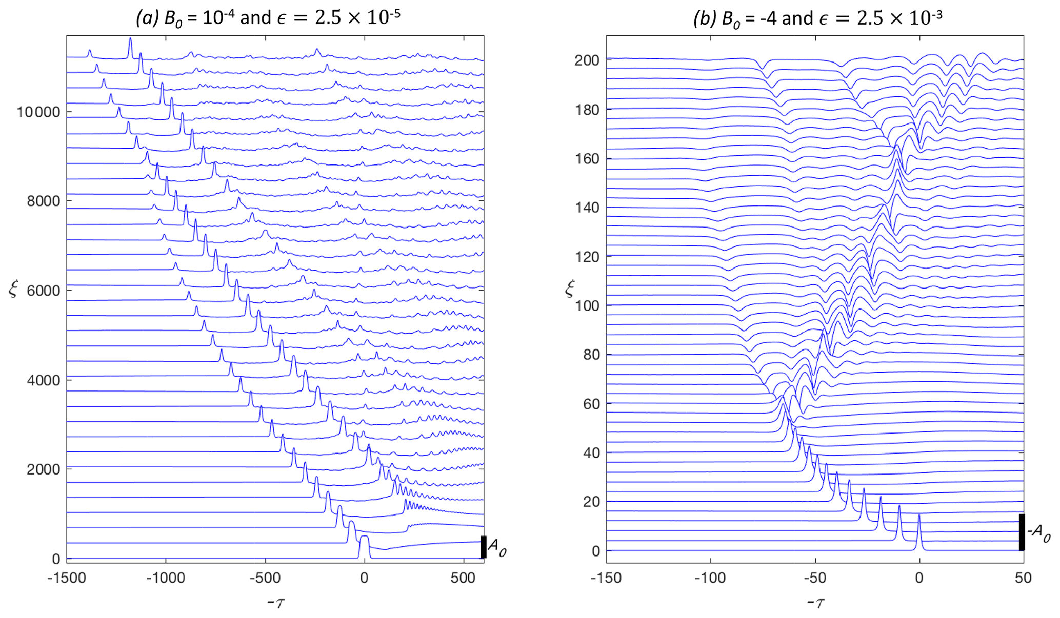
The complicated evolution of the decaying solitary wave and the trailing radiation is illustrated in Fig. 4a and b. Figure 4a is the $B_{\mathrm{0}}={\mathrm{10}}^{-\mathrm{4}}$ and $\mathit{ϵ}=\mathrm{2.5}\times {\mathrm{10}}^{-\mathrm{5}}$ example in Fig. 3b. As the initial solitary wave decays, the trailing radiation itself steepens to form a group of solitary-like waves that also decay by radiation damping. Over larger distances, this radiation will likely organize into one or more nonlinear wave packets, as found by Grimshaw and Helfrich (2008), for the rotating KdV equation, and Whitfield and Johnson (2015), in the rotating Gardner equation.

The example in Fig. 4b has $B_{\mathrm{0}}=-\mathrm{4}$ and $\mathit{ϵ}=\mathrm{2.5}\times {\mathrm{10}}^{-\mathrm{3}}$ (see Fig. 3d). For these parameters, the evolution is further complicated since the radiation decay ceases at ξ≈50 (=0.21X_eO) when the wave amplitude decays to the limiting amplitude $A_{\lim }=-\mathrm{2}\mathit{\alpha }/\mathit{\nu }=-\mathrm{2}$ in these scaled variables. The wave then rapidly forms what appears to be a small solitary wave of reversed polarity (B₀>1) and a trailing wave packet that has characteristics similar to the breather solutions of the Gardner equation. However, this packet subsequently disintegrates due to rotational effects. The complicated nature of the wave evolution with rotation in homogeneous conditions suggests even more interesting features when both rotation and inhomogeneous effects are active.

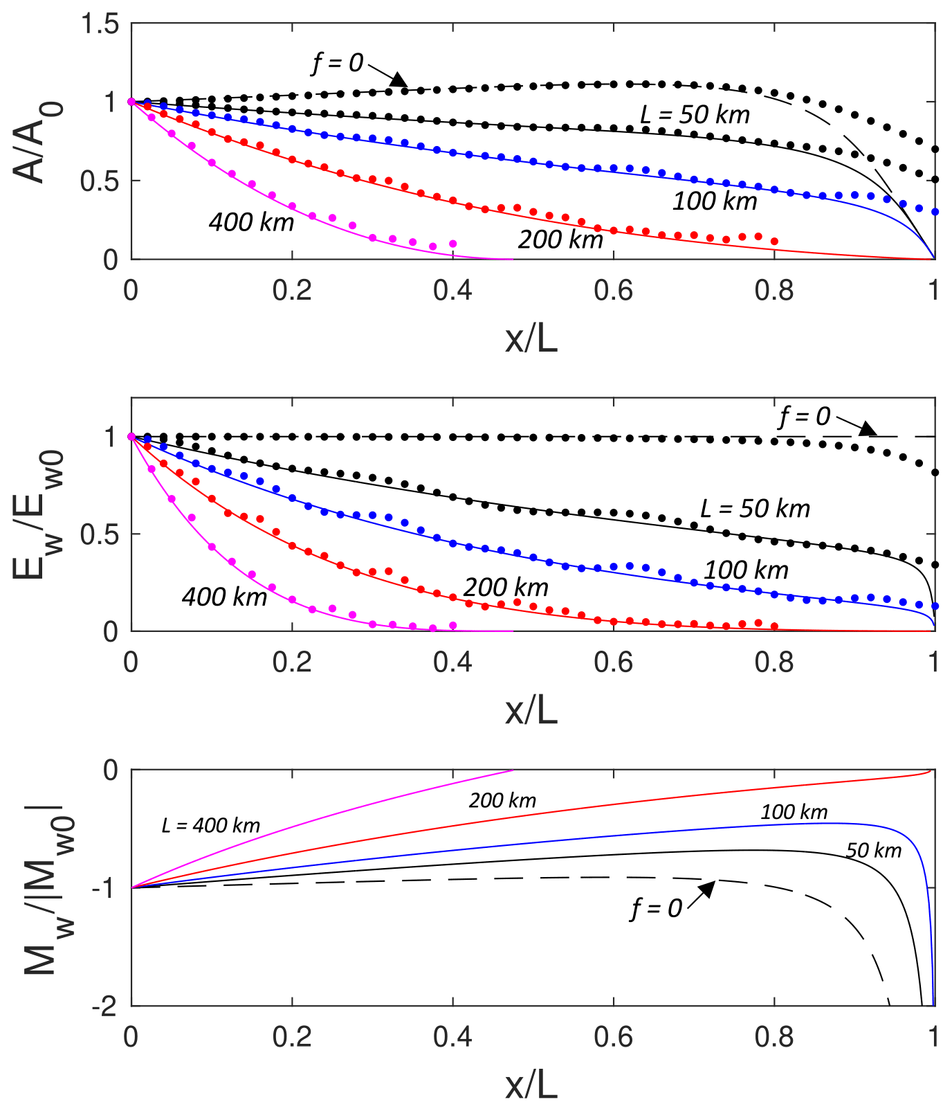
Figure 5 Adiabatic theory for wave propagation from deep to shallow in a two-layer system, with h₁=50 m, h₂₀=450 m, $g^{\prime }=\mathrm{0.005}$ m s⁻², $f={\mathrm{10}}^{-\mathrm{4}}$ s⁻¹, and $A_{\mathrm{0}}=-\mathrm{25}$ m. $A/A_{\mathrm{0}}$, $E_{\mathrm{w}}/E_{\mathrm{w}\mathrm{0}}$, and $M_{\mathrm{w}}/\left|M_{\mathrm{w}\mathrm{0}}\right|$ are shown as functions of $x/L$. The solid lines are for L=50 (black), 100 (blue), 200 (red), and 400 km (magenta). The dashed lines are for f=0. The dots are from the solutions of Eq. (3).

4.2 Combined inhomogeneous and rotation effects

Ostrovsky and Helfrich (2019) showed that, for the rKdV equation, the competition between extinction by radiation decay and the point of polarity reversal, α=0, could be characterized by the ratio of the inhomogeneous and rotation terms of Eq. (1) as follows:

$$\begin{array}{}\text{(31)}& C\approx {\displaystyle \frac{c}{\mathit{\gamma }}}{\displaystyle \frac{Q_x}{Q}}{\displaystyle \frac{{\mathit{\eta }}_x}{\mathit{\eta }}}\sim {\displaystyle \frac{c}{\mathit{\gamma }L\mathrm{\Delta }}}={\displaystyle \frac{X_{\mathrm{eO}}}{L}},\end{array}$$

where L is the length scale over which inhomogeneous term Q varies, e.g., the distance to the α=0 location. Δ is the solitary wave scale, which is taken above to be the KdV wave scale ${\mathrm{\Delta }}_{\mathrm{KdV}}=(\mathrm{12}\mathit{\beta }/A_{\mathrm{0}}\mathit{\alpha }{)}^{\mathrm{1}/\mathrm{2}}$. For C≫1, inhomogeneous effects dominate and conversely rotational decay dominates for C≪1. Alternatively, Δ might taken to be the Gardner solitary wave scale ${\mathrm{\Delta }}_G={\mathrm{\Delta }}_{\mathrm{KdV}}[\mathrm{2}/(\mathrm{1}+B_{\mathrm{0}}){]}^{\mathrm{1}/\mathrm{2}}$. However, for B₀>0 and not too large, the term in parentheses is O(1), and Eq. (31) is a reasonable scaling estimate. One could simply define $C=X_{\mathrm{eG}}/L$, but since $X_{\mathrm{eG}}/X_{\mathrm{eO}}\approx \mathrm{1}$ for $\mathrm{0}<B_{\mathrm{0}}<\mathrm{10}$ (see Fig. 1), this also gives C from Eq. (31). The exception is for situations with $B_{\mathrm{0}}<-\mathrm{1}$, since $X_{\mathrm{eG}}/X_{\mathrm{eO}}$ can be much less than one.

To illustrate the combined effects of inhomogeneity and rotation, a two-layer Boussinesq stratification with upper layer depth h₁, variable lower layer depth h₂(x), reduced gravity $g^{\prime }=g({\mathit{\rho }}_{\mathrm{2}}-{\mathit{\rho }}_{\mathrm{1}})/{\mathit{\rho }}_{\mathrm{1}}$, and Coriolis frequency f will be considered. Here ρ₁ and ρ₂ are the densities of the upper and lower layers, respectively. Relations for the coefficients α(x), ν(x), etc., are given in (A6). Note that ν<0 for two-layer stratifications. Thus, only the $\mathrm{0}<B_{\mathrm{0}}<\mathrm{1}$ branch of solitary wave solutions is possible. The wave polarity is given by the sign of α, with α<0 (>0) for $h_{\mathrm{1}}/h_{\mathrm{2}}<\mathrm{1}$ (>1).

Figure 6 rG numerical solutions for h₁=50 m, h₂₀=450 m, $g^{\prime }=\mathrm{0.005}$ m s⁻², $f={\mathrm{10}}^{-\mathrm{4}}$ s⁻¹, and $A_{\mathrm{0}}=-\mathrm{25}$ m. (a) L=50 km and (b) L=200 km. The wave amplitude η(x,t) is shown at $x/L$ as a function of normalized shifted time, $-s(g^{\prime }/H{)}^{\mathrm{1}/\mathrm{2}}$, where $H=h_{\mathrm{1}}+h_{\mathrm{20}}$. The initial wave amplitude is indicated by the scale on the lower right of each panel.

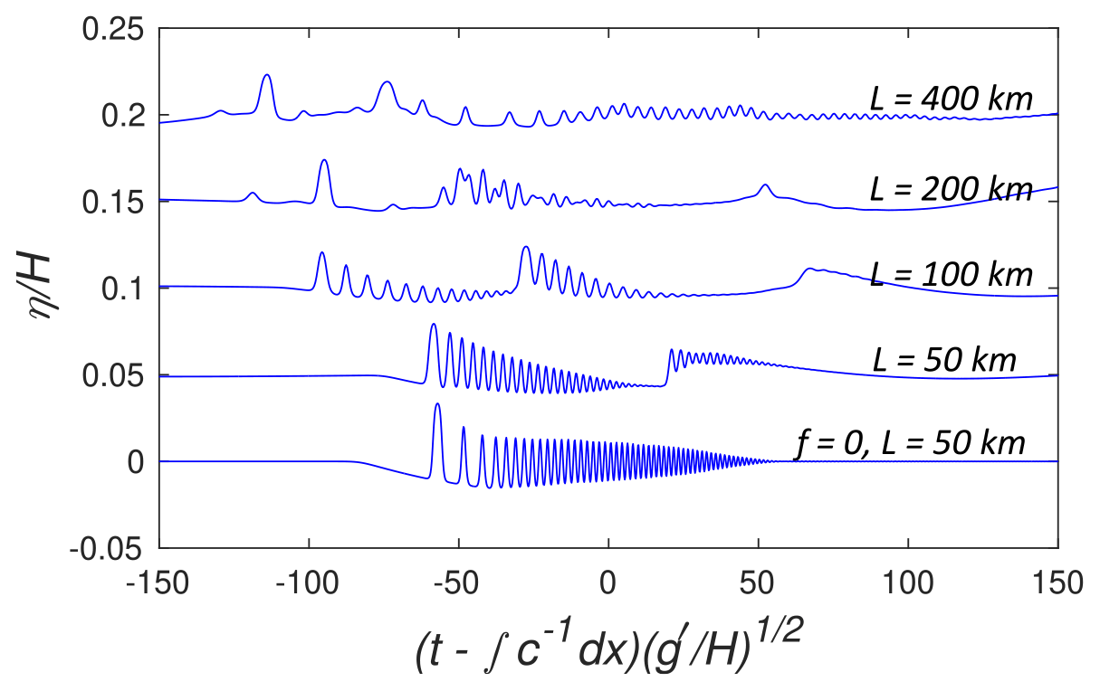
Figure 7 $\mathit{\eta }/H$ at $x/L=\mathrm{1.2}$ for the parameters of Fig. 5. The bottom curve is the non-rotating case with L=50 km. The top four lines include rotation and have L=50, 100, 200, and 400 km from bottom to top. The curves are offset by 0.05.

The bottom slope will be taken constant, and the lower layer depth is given by the following:

$$\begin{array}{}\text{(32)}& {\displaystyle \frac{h_{\mathrm{2}}\left(x\right)}{h_{\mathrm{20}}}}=\mathrm{1}-\left(\mathrm{1}-{\displaystyle \frac{h_{\mathrm{1}}}{h_{\mathrm{20}}}}\right){\displaystyle \frac{x}{L}},\end{array}$$

where h₂₀=h₂(0), and L is the distance from the origin to the critical point, where α=0 (i.e., h₁=h₂). The case $h_{\mathrm{1}}/h_{\mathrm{20}}<\mathrm{1}$ corresponds to an initial solitary wave, with A₀<0 propagating from deep to shallower water. The propagation of a positive wave, A₀>0, from shallow to deeper water occurs for $h_{\mathrm{1}}/h_{\mathrm{20}}>\mathrm{1}$. While the adiabatic solutions can be obtained only up to the critical point, x≤L, numerical solutions of the rG equation are found beyond the critical depth. In the deep-to-shallow situation, the bottom slope is continued until $h_{\mathrm{2}}=h_{\mathrm{1}}/\mathrm{2}$, beyond which h₂ is constant over a shelf region.

Note that the linear bottom slope in Eq. (32) will not allow for the interesting, but rather special, topographic conditions that Stepanyants (2019) found for the rKdV regime. In those cases, rotation and inhomogeneity effects can be balanced and give a constant soliton amplitude. However, there is no balance for fluid velocity and, more important, soliton energy, which still decreases due to radiation.

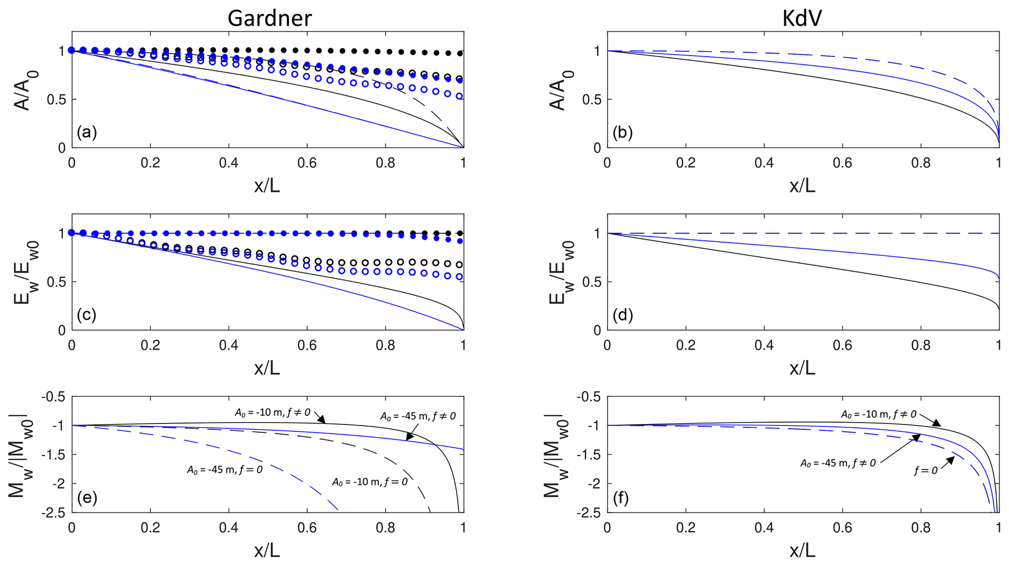
Figure 8 Adiabatic theory for wave propagation from deep to shallow in a two-layer system with h₁=100 m, h₂₀=200 m, $g^{\prime }=\mathrm{0.01}$ m s⁻², $f={\mathrm{10}}^{-\mathrm{4}}$ s⁻¹, and L=40 km. Panels (a, c, e) show $A/A_{\mathrm{0}}$, $E_{\mathrm{w}}/E_{\mathrm{w}\mathrm{0}}$ and $M_{\mathrm{w}}/\left|M_{\mathrm{w}\mathrm{0}}\right|$, for the rotating Gardner theory. The solid (dashed) lines are with (without) rotation for $A_{\mathrm{0}}=-\mathrm{10}$ m (black) and −45 m (blue). The open (solid) symbols are from the corresponding numerical solutions of Eq. (3) with (without) rotation. Panels (b, d, f) show the equivalent rotating KdV adiabatic solutions.

Figure 9 $\mathit{\eta }/H$ at $x/L=\mathrm{1.5}$ for the parameters of Fig. 8. (a) $A_{\mathrm{0}}=-\mathrm{10}$ m and (b) $A_{\mathrm{0}}=-\mathrm{45}$ m. The solid (dashed) lines are with (without) rotation.

The evolution of the wave amplitude A(x) is shown in Fig. 5a for a deep to shallow case for a representative oceanographic situation, with h₁=50 m, h₂₀=450 m, $g^{\prime }=\mathrm{0.005}$ m s⁻², $f={\mathrm{10}}^{-\mathrm{4}}$ s⁻¹, and $A_{\mathrm{0}}=-\mathrm{25}$ m. For this initial wave, B₀=0.764 so that effects of the cubic nonlinearity are present but do not dominate initially. Slope lengths $L=\mathrm{50},\mathrm{100},\mathrm{200}$, and 400 km are considered and give $C=\mathrm{3.46},\mathrm{1.73},\mathrm{0.86}$, and 0.43, respectively, from Eq. (31). The solid lines show the rotating adiabatic theory, and the dashed line shows the f=0 solution (equivalent for all L when plotted against $x/L$). As anticipated from the values of C, rotational decay effects increase significantly as L increases with complete, or nearly complete, extinction for the two longer slopes. However, even for L=50 km, rotation causes a noticeable reduction in wave amplitude compared to the non-rotating solution.

Figure 5b shows the wave energy, E_w(x) from Eq. (14), for the same parameters. The ratio $E_{\mathrm{w}}/E_{\mathrm{w}\mathrm{0}}$ is a measure of the fraction of initial wave energy that remains in the evolving solitary wave, with the difference lost to the trailing inertia–gravity wave radiation. Even for the shortest slope, L=50 km, where the effects of rotation were relatively weak, more than half of the initial wave energy is lost to inertia–gravity wave radiation by $x/L\approx \mathrm{0.8}$.

The variation in wave mass, M_w from Eq. (15), is plotted in Fig. 5c. In all cases, rotation causes an initial reduction in wave mass, which is compensated in the trailing radiation and emerging shelf (with the same mass sign as the initial wave). The mass goes to zero for the two longer slopes prior to the critical point, while for the two shorter slopes the wave mass increases rapidly as the critical point is approached, similar to the non-rotating result. However, increased slope length (i.e., rotational effects) delays this growth with consequences for the magnitude of the trailing shelf and the subsequent wave structure transmitted onto the topographic shelf (see below).

Also shown in Fig. 5a and b are the results from the numerical solutions to the rG equation (Eq. 3). The energy of the solitary wave in the rG model is found by integrating Qη² in a small region encompassing the solitary wave that does not incorporate an appreciable trailing radiation. The agreement is quite good for all the cases, except for $x/L\mathit{\gtrsim }\mathrm{0.8}$ and L=50 and 100, where the amplitude from the rG numerical calculation does not decay as rapidly as in the adiabatic model. This is consistent with previous studies without rotation (Grimshaw et al., 1998b, 1999). As the point of polarity reversal is approached, the wave elongates to form a rarefaction, and the trailing shelf with opposite polarity emerges. Figure 5 shows that the disagreement is associated with rapid changes in the wave amplitude and mass. In this region, that assumption of slow variation of the inhomogeneity fails.

There are two examples of the full rG solutions for L=50 and 200 km shown in Fig. 6, and the rG solutions at $x/L=\mathrm{1.2}$ for all five cases in Fig. 5 are compared in Fig. 7. Note that $h_{\mathrm{2}}=h_{\mathrm{1}}/\mathrm{2}$ for $x/L\ge \mathrm{1.0625}$ on the shelf. Again, even for L=50 km, the rotation leads to a clear effect on the wave signal transmitted on to the shelf as the leading crest of the (weak) trailing inertia–gravity wave also steepens to form a second transmitted wave packet. The second packet is consistent with the breaking criteria obtained by Grimshaw et al. (2012) and was similarly noted in Grimshaw et al. (2014). Further increases in the rotation effects lead to an additional transmitted packet for L=100 km. For the two longest slopes, L=200 and 400 km, the transmitted signal becomes increasingly disorganized. Figure 6b illustrates the evolution leading to this outcome. In this example, the initial solitary wave is extinguished before the critical point is reached. However, the trailing inertia–gravity wave steepens to produce a solitary wave that is itself scattered through the critical point. The interaction of the scattered signal with the trailing radiation gives rise to the observed disorganization. Recall that integration for calculating the energy of the leading wave, $E_{\mathrm{W}}=\int Q{\mathit{\eta }}^{\mathrm{2}}\mathrm{d}s$, shown in Fig. 5 by the red solid dots, only includes the leading solitary wave and not the secondary solitary wave that emerges from the trailing radiation.

In the examples above, the cubic nonlinearity was not an essential feature of the evolution. Indeed, the wave evolution is qualitatively similar to the rotating KdV solutions in Fig. 2 of Ostrovsky and Helfrich (2019). In Fig. 8, another example with h₁=100 m, h₂₀=200 m, $g^{\prime }=\mathrm{0.01}$ m s⁻², $f={\mathrm{10}}^{-\mathrm{4}}$ s⁻¹, and L=40 km is shown. Initial wave amplitudes of $A_{\mathrm{0}}=-\mathrm{10}$ and −45 m correspond to B₀=0.788 and 0.0478, respectively. The larger wave is very close to the limiting amplitude $A_{\lim }=-\mathrm{47.06}$ m. The competition parameters are C=4.56 and 9.68, respectively. The left column of Fig. 8 shows the rG adiabatic solutions, and for comparison, the right column shows the adiabatic solutions obtained from the rKdV theory (Eq. 18). Now the differences between the rG and rKdV solutions are substantial, especially for the large wave. The rKdV solution has this larger wave decaying more slowly than the smaller wave, while the rG model shows just the opposite. Similar to above, rotation, even for this relatively short slope (and hence weak rotational effect), causes significant energy loss in the primary wave as it climbs the slope. For $A_{\mathrm{0}}=-\mathrm{45}$ m, the mass M_w remains finite at the critical point, indicating the generation of a relatively weak trailing shelf. The agreement between the rG adiabatic model and the full rG solutions for A(x) is not very good, although the qualitative prediction that the large wave should decay more rapidly is found in both cases. The origin of the disagreement is likely due to the lack of separation between the wave scales and scale of the inhomogeneity.

The transmitted signals at $x/L=\mathrm{1.5}$ from the full rG numerical solutions with and without rotation are shown in Fig. 9. For both initial wave amplitudes, rotation leads to significant changes in the transmitted signal. This is especially true for $A_{\mathrm{0}}=-\mathrm{45}$ m, where the transmitted packet without rotation is replaced by a single, broad wave emerging onto the constant depth shelf with a much weaker trailing signal. However, on the shelf $A_{\lim }/H=\mathrm{0.0745}$, so that this leading wave must further adjust and is also subject to continued rotational decay.

5 Concluding remarks

In this paper we have continued a series of studies of nonlinear internal waves of a moderate amplitude in the shallow, stratified areas of the ocean (see the references in the Introduction). Based on the classical Korteweg–de Vries equation, we added the main factors, making the analysis closer to the physical reality, i.e., cubic nonlinearity, Earth's rotation, and sloping bottom. The interplay of these factors makes the problem rather complicated, both physically and mathematically. To better explain the qualitative effect of each of them, we first briefly reproduce the effect of rotation in the medium with quadratic nonlinearity (KdV with rotation), then that with both quadratic and cubic nonlinearities (Gardner with rotation), and, as the main content of this paper, the joint effect of rotation and inhomogeneity in the Gardner equation. The specific qualitative effect of the latter is the limiting soliton amplitude, and the corresponding increase in the wavelength so that the topography effect becomes especially important. Along with the approximate adiabatic approach, a direct numerical study of the rG equation was performed and confirmed the adiabatic theory and highlighted its limitations. This combined approach allowed us to demonstrate a rather complicated behavior of shoaling internal solitons. For example, whereas the soliton energy always decreases due to the radiation losses, the displacement amplitude and mass can increase in a shoaling wave at a finite distance due to the decrease in total depth. In turn, the oscillating tail reveals a complicated behavior that includes, in particular, the formation of nonlinear wave packets as in Grimshaw and Helfrich (2008), followed by an even more complex evolution. Another important point of bifurcation is that of the wave passage, through the condition h₁=h₂, when the polarity of a soliton is changed. According to the estimations, the interplay between the topography and rotation effects does exist under realistic oceanic conditions.

Future research should include further comparisons of the theory with observational results in different oceanic environments and extend the above results to the strongly nonlinear waves with rotation.

Appendix A: Coefficients of the rotating Gardner equation

The eigenvalue problem for the linear long wave phase speed c_n and vertical structure function for the isopycnal displacement Φ_n(z) of vertical mode n is, for the Boussinesq and rigid-lid limits (after dropping the subscript n), as follows:

$$\begin{array}{}\text{(A1)}& \begin{array}{rl}{\displaystyle \frac{d}{\mathrm{d}z}}& \left[{\left(c-\stackrel{\mathrm{‾}}{u}\right)}^{\mathrm{2}}{\displaystyle \frac{d\mathrm{\Phi }}{\mathrm{d}z}}\right]+N^{\mathrm{2}}\left(z\right)\mathrm{\Phi }=\mathrm{0},\\ & \mathrm{\Phi }(-h)=\mathrm{\Phi }\left(\mathrm{0}\right)=\mathrm{0}.\end{array}\end{array}$$

The buoyancy frequency is as follows:

$$\begin{array}{}\text{(A2)}& N^{\mathrm{2}}\left(z\right)=-{\displaystyle \frac{g}{{\mathit{\rho }}_{\mathrm{0}}}}{\displaystyle \frac{d\stackrel{\mathrm{‾}}{\mathit{\rho }}}{\mathrm{d}z}},\end{array}$$

where $\stackrel{\mathrm{‾}}{\mathit{\rho }}\left(z\right)$ is the background density profile, $\stackrel{\mathrm{‾}}{u}\left(z\right)$ is a background current in the direction of wave propagation, g is the gravitational acceleration, and ρ₀ is a reference density. From Grimshaw et al. (2004), the coefficients of the rG equation (Eq. 1) for a particular mode are given by the following:

$$\begin{array}{}\text{(A3a)}& {\displaystyle }I& {\displaystyle }=\mathrm{2}\underset{-h}{\overset{\mathrm{0}}{\int }}(c-\stackrel{\mathrm{‾}}{u}){\mathrm{\Phi }}^{\prime \mathrm{2}}\mathrm{d}z,\text{(A3b)}& {\displaystyle }\mathit{\alpha }& {\displaystyle }=I^{-\mathrm{1}}\underset{-h}{\overset{\mathrm{0}}{\int }}\mathrm{3}(c-\stackrel{\mathrm{‾}}{u}{)}^{\mathrm{2}}{\mathrm{\Phi }}^{\prime \mathrm{3}}\mathrm{d}z,\text{(A3c)}& {\displaystyle }\mathit{\beta }& {\displaystyle }=I^{-\mathrm{1}}\underset{-h}{\overset{\mathrm{0}}{\int }}(c-\stackrel{\mathrm{‾}}{u}{)}^{\mathrm{2}}{\mathrm{\Phi }}^{\mathrm{2}}\mathrm{d}z,\text{(A3d)}& {\displaystyle }Q& {\displaystyle }=c^{\mathrm{2}}I,\text{(A3e)}& {\displaystyle }\mathit{\gamma }& {\displaystyle }=I^{-\mathrm{1}}{f}^{\mathrm{2}}\underset{-h}{\overset{\mathrm{0}}{\int }}\left({\mathrm{\Phi }}^{\prime \mathrm{2}}-{\displaystyle \frac{{\stackrel{\mathrm{‾}}{u}}^{\prime }}{c-\stackrel{\mathrm{‾}}{u}}}\mathrm{\Phi }{\mathrm{\Phi }}^{\prime }\right)\mathrm{d}z.\end{array}$$

When $\stackrel{\mathrm{‾}}{u}=\mathrm{0}$, $\mathit{\gamma }=f^{\mathrm{2}}/\mathrm{2}c$, where f is the Coriolis frequency. The general relation for γ with ${\stackrel{\mathrm{‾}}{u}}^{\prime }\ne \mathrm{0}$ was derived by Alias et al. (2014). The coefficient of the cubic nonlinear term is given by the following:

$$\begin{array}{}\text{(A4)}& \begin{array}{rl}\mathit{\nu }& =I^{-\mathrm{1}}\underset{-h}{\overset{\mathrm{0}}{\int }}\left[\mathrm{3}(c-\stackrel{\mathrm{‾}}{u}{)}^{\mathrm{2}}\left(\mathrm{3}{T}_z-\mathrm{2}{\mathrm{\Phi }}^{\prime \mathrm{2}}\right){\mathrm{\Phi }}^{\prime \mathrm{2}}-{\mathit{\alpha }}^{\mathrm{2}}{\mathrm{\Phi }}^{\prime \mathrm{2}}\right.\\ & \left.+\mathit{\alpha }(c-\stackrel{\mathrm{‾}}{u})\left[\mathrm{5}{\mathrm{\Phi }}^{\prime \mathrm{2}}-\mathrm{4}{T}_z\right]{\mathrm{\Phi }}^{\prime }\right]\mathrm{d}z,\end{array}\end{array}$$

with the nonlinear correction to the vertical structure function, T(z), found from

$$\begin{array}{}\text{(A5)}& \begin{array}{rl}{\displaystyle \frac{d}{\mathrm{d}z}}& \left[{\left(c-\stackrel{\mathrm{‾}}{u}\right)}^{\mathrm{2}}{\displaystyle \frac{\mathrm{d}T}{\mathrm{d}z}}\right]+N^{\mathrm{2}}T=-\mathit{\alpha }{\displaystyle \frac{d}{\mathrm{d}z}}\left[(c-\stackrel{\mathrm{‾}}{u}){\displaystyle \frac{d\mathrm{\Phi }}{\mathrm{d}z}}\right]\\ & +{\displaystyle \frac{\mathrm{3}}{\mathrm{2}}}{\displaystyle \frac{d}{\mathrm{d}z}}\left[(c-\stackrel{\mathrm{‾}}{u}{)}^{\mathrm{2}}{\left({\displaystyle \frac{d\mathrm{\Phi }}{\mathrm{d}z}}\right)}^{\mathrm{2}}\right],\end{array}\end{array}$$

with $T(-h)=T\left(\mathrm{0}\right)=\mathrm{0}$. The solution T(z) is normalized through the addition of bΦ(z), with b chosen so that T(z_max)=0, where Φ(z_max)=1. This gives the isopycnal vertical displacement $\mathit{\xi }(x,z,t)=\mathit{\eta }(x,t)\mathrm{\Phi }\left(z\right)+{\mathit{\eta }}^{\mathrm{2}}(x,t)T\left(z\right)$.

In a two-layered stratification, with depths h₁ and h₂ of the upper and lower layers, respectively, and $\stackrel{\mathrm{‾}}{u}=\mathrm{0}$, the following applies:

$$\begin{array}{}\text{(A6)}& \begin{array}{rl}& c^{\mathrm{2}}=g^{\prime }{\displaystyle \frac{h_{\mathrm{1}}{h}_{\mathrm{2}}}{h_{\mathrm{1}}+h_{\mathrm{2}}}},\mathit{\alpha }={\displaystyle \frac{\mathrm{3}c}{\mathrm{2}}}{\displaystyle \frac{h_{\mathrm{1}}-h_{\mathrm{2}}}{h_{\mathrm{1}}{h}_{\mathrm{2}}}},\\ & \mathit{\nu }=-{\displaystyle \frac{\mathrm{3}c}{\mathrm{8}}}{\displaystyle \frac{\left(h_{\mathrm{1}}^{\mathrm{2}}+\mathrm{6}{h}_{\mathrm{1}}{h}_{\mathrm{2}}+h_{\mathrm{2}}^{\mathrm{2}}\right)}{(h_{\mathrm{1}}{h}_{\mathrm{2}}{)}^{\mathrm{2}}}},\\ & \mathit{\beta }={\displaystyle \frac{c}{\mathrm{6}}}{h}_{\mathrm{1}}{h}_{\mathrm{2}},\mathit{\gamma }={\displaystyle \frac{f^{\mathrm{2}}}{\mathrm{2}c}},Q=\mathrm{2}{g}^{\prime }c.\end{array}\end{array}$$

Here $g^{\prime }=g\mathrm{\Delta }\mathit{\rho }/{\mathit{\rho }}_{\mathrm{0}}$, and $\mathrm{\Delta }\mathit{\rho }={\mathit{\rho }}_{\mathrm{2}}-{\mathit{\rho }}_{\mathrm{1}}$ is the difference in densities between the lower and upper layers.