Control simulation experiment with Lorenz's butterfly attractor

In numerical weather prediction (NWP), sensitivity to initial conditions brings chaotic behaviors and an intrinsic limit to predictability, but it also implies an effective control in which a small control signal grows rapidly to make a substantial difference. The Observing Systems Simulation Experiment (OSSE) is a well-known approach to study predictability, where “nature” is synthesized by an independent NWP model run. In this study, we extend the OSSE and design the control simulation experiment (CSE), where we apply a small signal to control “nature”. Idealized experiments with the Lorenz-63 three-variable system show that we can control “nature” to stay in a chosen regime without shifting to the other, i.e., in a chosen wing of Lorenz's butterfly attractor, by adding small perturbations to “nature”. Using longer-lead-time forecasts, we achieve more effective control with a perturbation size of less than only 3 % of the observation error. We anticipate our idealized CSE to be a starting point for a realistic CSE using the real-world NWP systems, toward possible future applications to reduce weather disaster risks. The CSE may be applied to other chaotic systems beyond NWP.

1 Introduction

The “butterfly effect”, discovered by Lorenz in the 1960s (Lorenz, 1963, 1993), is a phenomenon that an infinitesimal perturbation like “a butterfly flapping its wings in Brazil” causes a big consequence like “a tornado in Texas”. This extreme sensitivity brings chaotic behaviors and an intrinsic limit to predictability, but it also allows us to design an effective control which was explored as “the control of chaos” in the 1990s (e.g., a review by Boccaletti et al., 2000). That is, we could take advantage of the “butterfly effect” and design an effective control with a series of infinitesimal interventions leading to a desired future. The control of weather is humans' long-time desire, and if we know when and where to put a “butterfly”, we could lead a better life by, for example, reducing the risks of tornadoes.

Predictability has been studied extensively, and we enjoy current high-quality weather prediction that is consistently being improved. However, studies on controllability are limited because we had to first improve the prediction accuracy and because our engineering power may be insufficient to enforce large enough perturbations to the atmosphere. Based on recent high-quality numerical weather prediction (NWP), this study attempts to explore a computational simulation approach to weather controllability. The simulation studies reveal what perturbations are needed to modify and control the weather. Mutual interactions between the simulation studies and the intervention techniques would be essential for future developments toward real-world applications.

Previous efforts in weather modification include rain enhancement studies (e.g., a review by Flossmann et al., 2019) by cloud seeding with ground-based facilities and aircraft injecting smokes and dry ices into moist air, so that the aerosols act as cloud condensation nuclei and enhance cloud formation. These studies greatly helped advance our knowledge about physical processes of clouds and precipitation, but in terms of controlling the weather, we had only limited success with unclear implications for high-impact weather events, mainly because this method works only with supersaturated air. On the climate scale, geoengineering is a widely discussed concept, such as launching mirror satellites to reflect the sunlight and injecting dusts into the stratosphere to block the sunlight to cool the air. Li et al. (2018) performed computational simulations and explored potential rain enhancements in the Sahel region by implementing large-scale wind and solar farms over the Sahara and modulating the global atmospheric circulation. However, actual geoengineering operations are controversial because they may cause irreversible unexpected side-effects due to our limited knowledge of the Earth system. The accepted and currently ongoing operations to counteract the current climate change may be limited in reducing the greenhouse gas emissions and enhancing renewables and recycles.

Our focus here is different. We aim to apply “the control of chaos” to the weather. We do not aim to cause a permanent irreversible change to nature, but we would like to control the weather within its natural variability and to aid human activities, for example, by shifting the location of an extreme rain region to avoid disasters without causing a side-effect on the global climate. For extreme weather that occurs in a chaotic manner under natural variations, the control of chaos suggests that proper infinitesimal perturbations to the natural atmosphere alter the orbit of the atmospheric dynamics to a desired direction. If the proper infinitesimal perturbations are within our engineering capability, we could apply the control in the real world. However, we cannot be too cautious about potential side-effects and must consider and address every possible consequence. We will come back to this issue later in conclusion.

Here we develop a method of the control simulation experiment (CSE). It would be straightforward to extend the method to broader fields with chaotic dynamics beyond NWP. Weather prediction has been improved consistently by studying predictability and better initial conditions for NWP. Data assimilation (DA) combines the NWP model and observation data for optimal prediction. The method of DA shares that of optimal control, such as the Kalman filter (Kalman, 1960), where prediction and control are the two sides of a coin. DA has been studied extensively to improve the prediction, and this study illuminates the control.

The Observing Systems Simulation Experiment (OSSE) is a powerful method to simulate an NWP system (e.g., Atlas, 1985; Hoffmann and Atlas, 2016). The OSSE can be designed to assess the impact of certain observing systems and is useful, for example, for evaluating the potential value of a new satellite sensor before launch. The OSSE can also be designed to evaluate DA methods. In the OSSE, an independent model run acts as a synthetic “nature run” (NR), and we simulate observations by sampling the NR. The NWP system is blind to the NR, takes the simulated observations, and estimates the NR. We compare the estimation accuracy among different OSSEs with different observations and different DA methods.

Here we extend the OSSE and apply small perturbations to the NR to alter the orbit to a desired direction. Investigating effective perturbations would address the controllability. As a proof of concept, we focus on the essence of the problem and use Lorenz's three-variable model (L63, Lorenz, 1963) instead of using a complex large-scale NWP model. In predictability studies, OSSEs are often performed with such simple idealized models like L63 to explore new DA methods before application to real NWP models (e.g., Kalnay et al., 2007; Yang et al., 2012). L63 is often used to focus on the essence of the problem since L63 shows typical chaotic behaviors, with the solution manifold being a well-known “butterfly attractor” (Fig. 1a), which has two regimes or wings corresponding to the positive and negative values for variable x. The regime shifts randomly, and the predictability is limited due to chaos. Evans et al. (2004) revealed predictability of the regime shift from rapidly growing uncertainties given by the growth rate of specific growing perturbations known as the bred vectors (Toth and Kalnay, 1993).

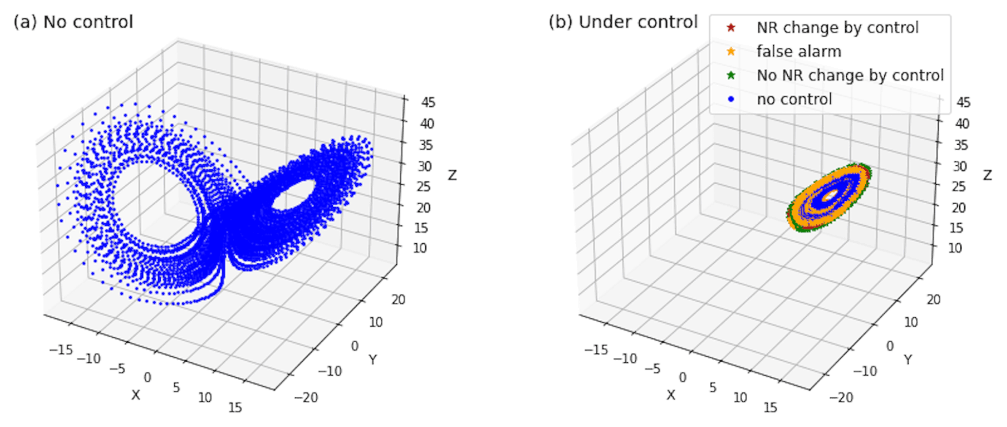
Figure 1 Phase space of the three-variable Lorenz model. (a) Lorenz's butterfly attractor from the NR without control; (b) the NR under control (D=0.05, T=⌈4T₀⌉). Each dot shows every time step for 8000 steps. See also a movie at https://doi.org/10.5446/54893.

2 Experiments

We first perform a regular OSSE following the previous studies (Kalnay et al., 2007; Yang et al., 2012). The L63 system with the standard choice of the parameters (Lorenz, 1963) is discretized in time by the Runge–Kutta fourth-order scheme with a time step of 0.01 units. We define one step as 0.01 units throughout the paper. We assimilate observations every T_a=8 steps. A round of the orbit, i.e., from a maximum to the next maximum for variable x, corresponds to T₀=75.1 steps on average. We use the ensemble Kalman filter (EnKF, e.g., Evensen, 1994; Houtekamer and Zhang, 2016) with three ensemble members, which represent equally probable state estimates. For simplicity, we observe all three variables in this study but any subset of observations except for observing only z variable results in the same conclusion, as suggested by the previous study on chaos synchronization (Yang et al., 2006). The observation noise is generated from the normal distribution for each variable independently with the variance of 2.0. The EnKF results in an accurate state estimation of the root mean square error (RMSE) of 0.32, consistent with the previous studies.

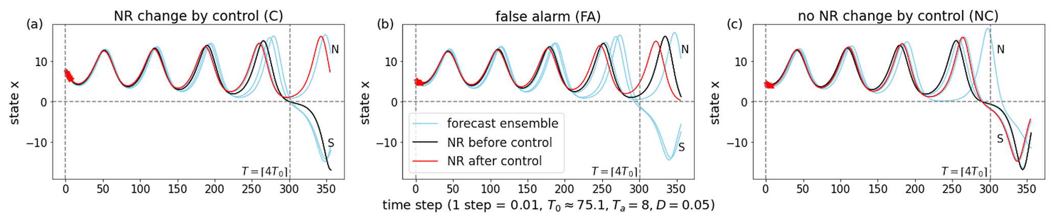
Figure 2 Control cases with T=⌈4T₀⌉ and D=0.05 for (a) NR changed (C), (b) false alarm (FA), and (c) NR unchanged (NC). Red ticks at the beginning (t=1,…,7) show addition of perturbations to the NR.

Next, we extend the OSSE and design a CSE. The goal of the control is to stay in a wing of the butterfly attractor without shifting to the other. It is essential that our prediction and control system is blind to the NR and takes only the imperfect observations. The control system finds when and what perturbations to add to the NR as follows (cf. Fig. 2).

1. Perform a DA update using the observations at time t (t=0 in Fig. 2).

2. Run an ensemble forecast for T steps from time t to t+T (T=⌈4T₀⌉ in Fig. 2, where ⌈ ⌉ indicates rounding up to the closest integer since the model integration is discretized).

3. If at least one ensemble member shows the regime shift, activate the control (step 4); otherwise, go to step 1 for the next DA at time t+T_a.

4. Add perturbations with Euclidean norm D to the NR at every step from t+1 to $t+T_{\mathrm{a}}-\mathrm{1}$. More precisely, at time t+i (i=1,…,T_a−1), the NR state is evolved from the previous NR state at time $t+i-\mathrm{1}$ and is perturbed by adding (dx, dy, dz), where $\sqrt{\mathrm{d}{x}^{\mathrm{2}}+\mathrm{d}{y}^{\mathrm{2}}+\mathrm{d}{z}^{\mathrm{2}}}=D$ (Fig. 2 red ticks, indicating perturbations added to the NR with D=0.05).

5. At time t+T_a, the new NR is used to simulate the observations; go to step 1 for the next DA at time t+T_a.

Step 4 requires perturbations added to the NR. Investigating different strategies to generate the perturbations addresses controllability. Randomly chosen perturbations are found to be ineffective, but instead we find the following strategy effective. We choose an ensemble member “S” showing the regime shift and another ensemble member “N” not showing the regime shift. If all three ensemble members show the regime shift, we use the ensemble members from the former initial times for an extended forecasting period and identify an ensemble member “N” not showing the regime shift during the period from t to t+T. Take the differences of the two ensemble members S − N for every step from t+1 to $t+T_{\mathrm{a}}-\mathrm{1}$ (1 to 7 in Fig. 2) before the next observations are available at t+T_a (8 in Fig. 2). The differences are used as perturbations added to the NR at appropriate time steps. Here, we consider the limitation of our intervention and include only a subset of the three variables (x, y, z) with a limited perturbation size. The choice of the variables and norm D are the parameters for intervention.

Figure 2 illustrates three different cases with perturbations added to all three variables (x, y, z) with D=0.05 and T=⌈4T₀⌉. With these settings the control is successful, as shown in Fig. 1b for 8000 steps. Figure 2a shows the case in which the NR is changed by the control and stays in the positive-x regime successfully (simply “C”​​​​​​​ for change). Figure 2b shows the case of a false alarm (FA), in which the NR does not show the regime shift but the ensemble prediction does. Therefore, the perturbations are added unnecessarily but do not hurt. Figure 2c shows the case in which the NR is not changed by control and still shows the regime shift (simply “NC” for no change).

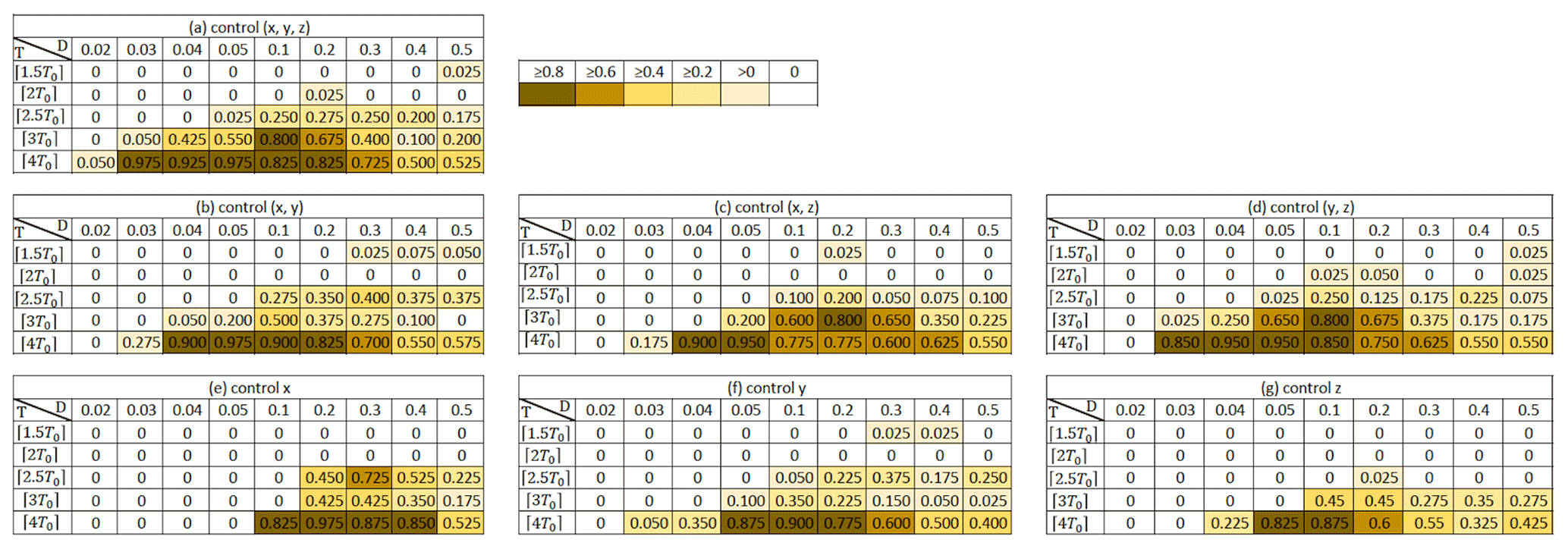
Figure 3 Rates of successful control out of 40 CSEs for perturbations added to variables (a) x, y, z, (b) x, y, (c) x, z, (d) y, z, (e) x, (f) y, and (g) z.

To investigate the sensitivity to the parameters T and D and the choice of the perturbed variables, we perform 40 independent experiments for each setting for 8000 steps (1000 DA cycles; cf. Appendix A for the exact choices of the initial conditions) and count the number of successful experiments in which the NR stays in a single regime under control. Higher success rates correspond to better controllability. With longer forecasts (larger T), control is generally more effective (Fig. 3). With small T<⌈2.5T₀⌉, the success rates are very low. The mean transition time for the regime shift is approximately 2.3T₀, which may be the minimum forecast length for effective control. With very small perturbations (D=0.02), the control is difficult, but a larger D does not necessarily improve the success rate. The perturbations are added every step, and the state evolves by approximately 0.5 (Euclidean norm) in one step on average (Table 1). This is about half of the evolution without control, suggesting that the perturbations effectively drag the NR states toward more stable regions of the attractor (cf. Fig. 1 and a movie at https://doi.org/10.5446/54893). Adding larger perturbations with a similar size to the one-step model evolution tends to reduce the effect of control. Although observing only z is not sufficient for DA, it is good for control. Perturbing only one variable y or z is effective with T=⌈4T₀⌉ and D>0.04, only an eighth of the analysis error of 0.32 or only 3 % of the observation error standard deviation of $\sqrt{\mathrm{2}}$. In short, the L63 regime change is considerably controllable.

Table 1 Averaged one-step model evolution in the Euclidean norm (OME) and the relative size of perturbations ($D/$OME). Only successful control cases are considered for CSEs with T=⌈4T₀⌉ and perturbations added to variables x, y, and z. “NA” indicates not available.

We further investigate the rates of FAs and NR changed (C) and unchanged (NC) by perturbations (Fig. 4a). With larger D, we find generally fewer interventions. With smaller D, we have more interventions mostly by FA. With smaller D, higher rates of NC suggest that longer-term small interventions are needed. Additional experiments by not applying FA and/or NC perturbations reveal the relative importance of these perturbations (Fig. 4b). These experiments require knowing the NR T steps in advance and therefore are not practical but are useful for understanding the roles of these perturbations. For D=0.2 and smaller, not applying FA perturbations does not significantly contribute to the control (Fig. 4b, yellow), whereas not applying NC has a significant impact on reducing the effect of control (Fig. 4b, blue, green). That is, the accumulation of NC perturbations would be essential for effective control. With large D>0.2, not applying FA and NC perturbations significantly enhances the effect of control (Fig. 4b, green). With the perturbation size similar to or even larger than the one-step model evolution (Table 1), a single instance of C perturbations is quite significant. In these cases, FA and NC perturbations are found to be harmful.

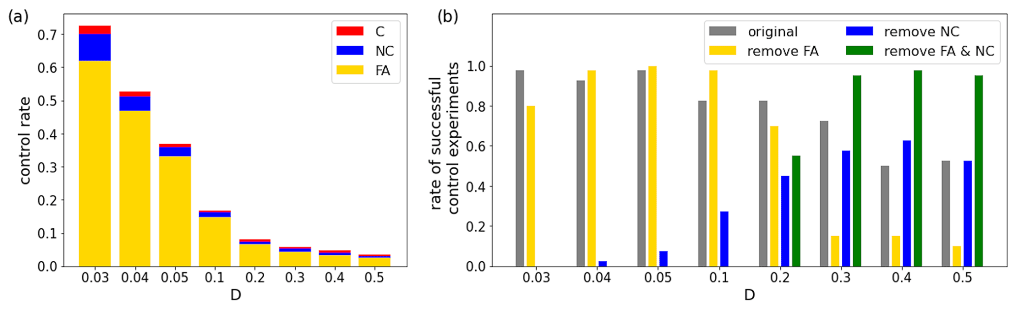
Figure 4 (a) Rates of the cases of C (red), FA (yellow), and NC (blue) for the successful control experiments with T=⌈4T₀⌉ and perturbations added to variables x, y, and z. The rates indicate the number of cases out of a total of 1000 DA cycles. (b) Rates of successful control experiments with T=⌈4T₀⌉ and perturbations added to variables x, y, and z for the original CSE (grey; cf. Fig. 3a), the CSE without applying FA perturbations (yellow), the CSE without applying NC perturbations (blue), and the CSE without applying FA and NC perturbations (green).

Finally, we perform additional sensitivity experiments with a longer DA interval of T_a=25 steps and with partial observations; i.e., only one or two variables are observed. The results generally agree with what has been shown so far (cf. Appendix B).

3 Conclusions

In this study, we proposed the CSE with numerical demonstration using the L63 three-variable model. The OSSE is a well-known, powerful approach to study predictability and to evaluate DA methods and observing systems without having real-world observation data. The CSE is an extension to the OSSE to study controllability and can be applied to various dynamical systems including full-scale NWP models. Our future studies apply the CSE to more complex models and investigate different control scenarios such as controlling the occurrences of extreme events. Such studies will address critical issues like how manageable interventions in terms of cost and energy can make differences to extreme events. This study is only a small step toward broad investigations that may lead to effective control of weather events.

As we described in the introduction, any real-world application requires extensive caution. For the case of the L63 model, one side of the attractor may not be desirable for all aspects. We must consider and assess every potential impact caused by the control and have proper protocols for social, ethical, and legal agreement about real-world operations.

Appendix A: The initial conditions of 40 CSEs

The​​​​​​​ OSSE with the L63 model follows that of the previous studies (Kalnay et al., 2007; Yang et al., 2012; Miller et al., 1994; Evensen, 1997). Here we describe the additional details that were not provided in the previous papers but that are necessary to repeat the experiment in this study. The initial condition for the NR was chosen to be (x, y, z) = (8.20747939, 10.0860429, 23.86324441) after running the L63 model for 1000 steps initialized by the three state variables taken from independent random draws from a normal distribution with mean 0 and variance 2.0. The NR was 8 million steps long, and the OSSE was performed for the same period as the NR.

The CSEs were performed for a total of 378 combinations of T, D, and the choice of intervention. There were nine, five, and seven choices of T, D, and intervention, as shown in Fig. 3. For each combination, 40 independent CSEs were performed for 8000 steps. The initial conditions for the 40 CSEs were chosen from the analyzed states of the OSSE at different time points as shown in Table A1. Figure 1b shows CSE no. 1 and Fig. 1a the corresponding period of the NR.

Table A1 Time points of the NR providing the initial conditions of the 40 independent CSEs. The initial time point coincides with the time when observations are available, i.e., only every T_a=8 steps, and the formula underneath the table provides the exact initial time point from the value in the table for a given parameter of T.

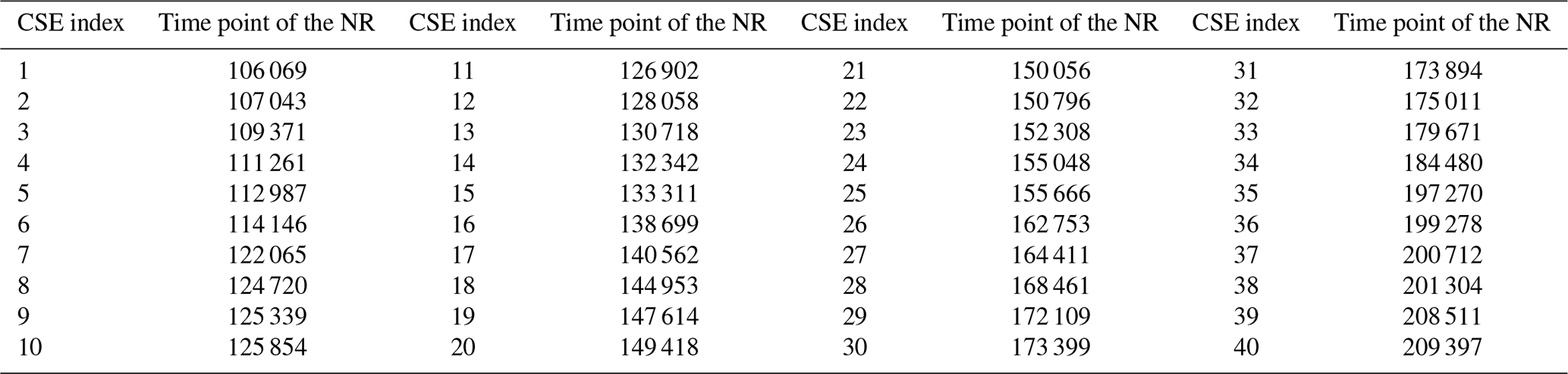
Initial time point = time point of the NR − T − [(time point of the NR − T) mod T_a].

Appendix B: Additional sensitivity experiments

CSEs​​​​​​​ are performed with a longer DA interval of T_a=25 steps, which results in an RMSE of 0.76, consistent with the previous studies. The results are generally consistent (Fig. B1 compared with Fig. 3).

CSEs are performed with different observing coverages, and the results are summarized in Table B1. Multiplicative inflation is manually tuned for each observing coverage.

Figure B1 Similar to Fig. 3 but for the case with a longer DA interval of T_a=25.

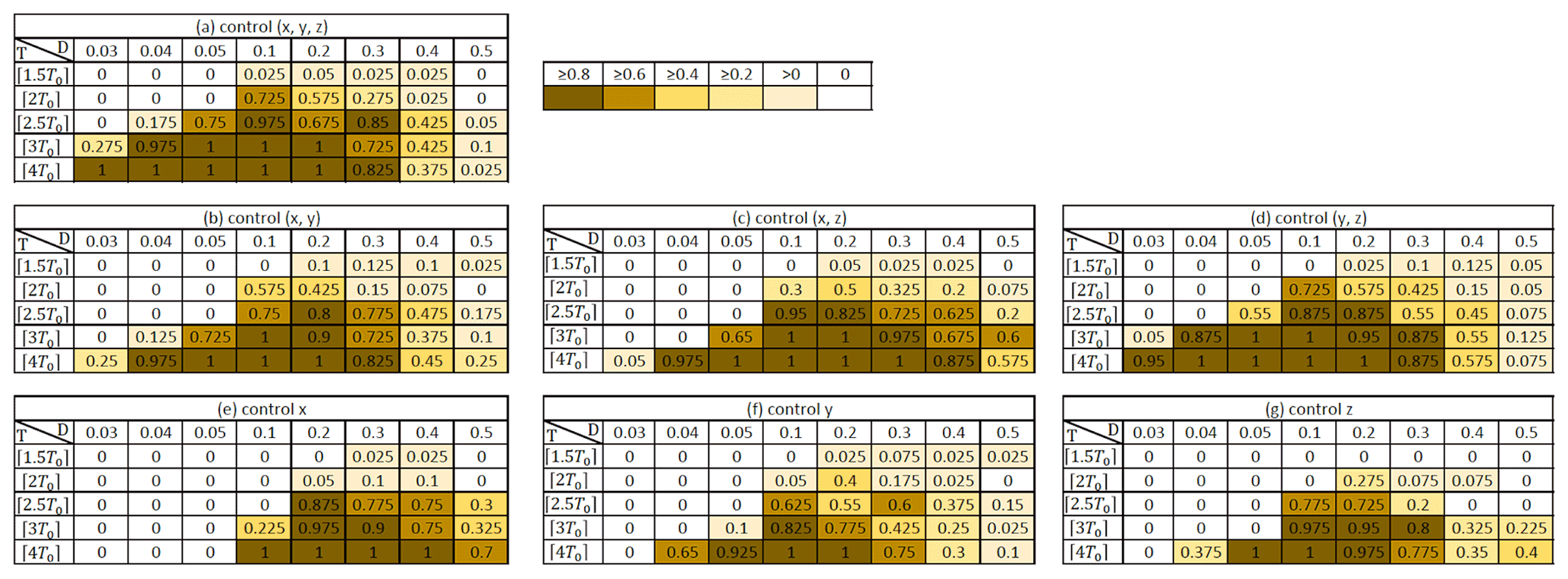
Table B1 Rates of successful control out of 40 CSEs with different observing coverage. T=⌈4T₀⌉ and perturbations are added to variables x, y, and z.