Inferring the instability of a dynamical system from the skill of data assimilation exercises

Data assimilation (DA) aims at optimally merging observational data and model outputs to create a coherent statistical and dynamical picture of the system under investigation. Indeed, DA aims at minimizing the effect of observational and model error and at distilling the correct ingredients of its dynamics. DA is of critical importance for the analysis of systems featuring sensitive dependence on the initial conditions, as chaos wins over any finitely accurate knowledge of the state of the system, even in absence of model error. Clearly, the skill of DA is guided by the properties of dynamical system under investigation, as merging optimally observational data and model outputs is harder when strong instabilities are present. In this paper we reverse the usual angle on the problem and show that it is indeed possible to use the skill of DA to infer some basic properties of the tangent space of the system, which may be hard to compute in very high-dimensional systems. Here, we focus our attention on the first Lyapunov exponent and the Kolmogorov–Sinai entropy and perform numerical experiments on the Vissio–Lucarini 2020 model, a recently proposed generalization of the Lorenz 1996 model that is able to describe in a simple yet meaningful way the interplay between dynamical and thermodynamical variables.

1 Introduction

We split the Introduction into three parts. The first two are proper introductory discussions providing the context. In part three, we provide the motivations and describe the goals of the present work.

1.1 Lyapunov vectors and related measures of chaos in a nutshell

The dynamics of several natural systems, including the atmosphere and the ocean, are characterized by chaotic conditions which, roughly speaking, describe the property that a system has sensitivity to initial states. This means that, even in the presence of a perfect model, small errors in the initial conditions will grow in size with time, until the forecast becomes de facto useless (Kalnay, 2002)¹. A mathematically sound technique for studying the sensitivity to initial conditions of a system amounts to studying the properties of its tangent space. In particular, under fairly general mathematical conditions for a deterministic n-dimensional system whose asymptotic dynamics takes place in a compact attractor, one can define n Lyapunov exponents (LEs) ${\mathit{\lambda }}_{\mathrm{1}},\mathrm{\dots },{\mathit{\lambda }}_n$, which are the asymptotic rates of amplification or decay of infinitesimally small perturbations with respect to a reference trajectory. Usually, the LEs are ordered according to their value, with λ₁ being the largest. Unless the system feature symmetries, all the LEs are distinct, and in the case of continuous time dynamics, one of them vanishes correspondingly to the direction of the flow and defines the neutral tangent space. Once ordered from the largest to the smallest, the sum of the first k LEs gives the asymptotic growth rate of a k-volume element defined by k displaced infinitesimally nearby the reference trajectory plus the reference trajectory itself. Additionally, if ${\mathit{\lambda }}_{n_{\mathrm{0}}}$ denotes the smallest non-negative LE, in many practical applications one can estimate the Kolmogorov–Sinai entropy (or metric entropy) σ_KS, which defines the rate of creation of information of the system due to its instabilities, as ${\mathit{\sigma }}_{\text{KS}}={\sum }_{i=\mathrm{1}}^{n_{\mathrm{0}}}{\mathit{\lambda }}_i$ (Pesin's identity). Finally, it is possible to use the spectrum of LEs to define a notion of dimension for the attractor of a chaotic system. The Kaplan–Yorke conjecture, which follows from the estimate of the rate of growth of the infinitesimal k volume, indicates that the information dimension of a chaotic attractor is given by $D_{\text{KY}}=p+{\sum }_{i=\mathrm{1}}^p{\mathit{\lambda }}_i/\left|{\mathit{\lambda }}_{p+\mathrm{1}}\right|$, where p is the largest index such that ${\sum }_{i=\mathrm{1}}^p{\mathit{\lambda }}_i\ge \mathrm{0}$. In systems where the phase space contracts (the large class of dissipative systems), one has D_KY<n. Roughly speaking, larger values of λ₁, of σ_KS, and of D_KY are associated with conditions of high instability and low predictability for the flow. This is clearly an extremely informal presentation of some of the features and properties of the LE; see Eckmann and Ruelle (1985) for a now classic discussion of these topics.

It is possible to associate each LE with a physical mode. Ruelle (1979) proposed the idea of performing a covariant splitting of the tangent linear space such that the basis vectors are actual trajectories of linear perturbations. The average growth rate of each of the covariant Lyapunov vector (CLVs) equals one of the LE. This idea was first implemented by Trevisan and Pancotti (1998) for studying the properties of the Lorenz 1963 model (Lorenz, 1963). Separate algorithms for the computation of CLVs were proposed in Ginelli et al. (2007) and Wolfe and Samelson (2007); see the recent comprehensive review by Froyland et al. (2013). Note that the CLVs corresponding to the positive (negative) LEs span the unstable (stable) tangent space. Recently, Lyapunov analysis of the tangent space was the subject of a special issue edited by Cencini and Ginelli (2013) and the book by Pikovsky and Politi (2016). Detailed Lyapunov analyses of geophysical flows on models of various levels of complexity have been recently reported (e.g. Schubert and Lucarini, 2015; Vannitsem and Lucarini, 2016; Vannitsem, 2017; De Cruz et al., 2018).

1.2 Data assimilation in chaotic systems: the signature and the use of chaos

The properties of the dynamical models have large implications on data assimilation (DA; Asch et al., 2016). Data assimilation refers to the family of theoretical and numerical methods that optimally combine data with a dynamical model with the goal of improving the understanding of the phenomenon under study, enhancing the prediction skill, and quantifying the associated uncertainty. Data assimilation has long been studied and developed in the geosciences. It is an unavoidable piece of the operational numerical weather prediction workflow, but it is nowadays used in a growing range of scientific areas (Carrassi et al., 2018).

Numerical and analytic evidence has emerged recently showing that under certain observational conditions (data types, spatio-temporal distribution, and accuracy), the performance of DA with chaotic dynamics relates directly to the instability properties of the dynamical model where data are assimilated. One can thus in principle use the knowledge of the dynamical features to inform not only the design of the DA that better suits the specific application – e.g. how many model realizations for the Monte Carlo based DA methods, or the length of the assimilation window in variational DA – but also the best possible observational deployment.

A stream of research has shed light on the mechanisms driving the response of the ensemble-based DA (Evensen, 2009), i.e. its functioning and suitability, when applied to chaotic systems. A recent comprehensive review can be found in Carrassi et al. (2022), while we succinctly recall the main findings in the following. In the deterministic linear and Gaussian case with a Kalman filter (KF) and smoother (KS), it has been analytically proved that the error covariance matrices converge in time onto the model's unstable–neutral subspace, i.e. the span of the backward Lyapunov vectors (BLVs) or of the covariant Lyapunov vectors (CLVs), associated with the non-negative LEs (Bocquet et al., 2017; Bocquet and Carrassi, 2017). These results have been shown numerically to hold for the ensemble Kalman filter/smoother in weakly non-linear regimes (EnKF/EnKS; Evensen, 2009) by Bocquet and Carrassi (2017). In practice, for sufficiently well observed scenarios, the error of the state estimate is fully confined within the unstable–neutral subspace. Because this subspace is usually much smaller than the full system's phase space, the above convergence results imply that an ensemble size as large as the unstable–neutral subspace dimension, n₀, suffices to achieve satisfactorily performance, i.e. to track the “truth” and effectively reduce the estimation error along with a substantial computational saving. The impact of instabilities on non-linear DA, in particular particle filters (PFs, see e.g. Van Leeuwen et al., 2019), has been recently elucidated in Carrassi et al. (2022): the number of particles needed to reach convergence depends on the size of the unstable–neutral subspace rather than the observation vector size.

The picture above slightly changes in the presence of a degenerate spectrum of LEs, which often arises in systems with multiple scales, associated with the presence of coupling between subsystems with different characteristic dynamical timescales (Vannitsem and Lucarini, 2016; De Cruz et al., 2018). The degeneracy is usually concentrated on the unstable–neutral portion of the LE spectrum. In these cases it is necessary to increase the ensemble size to account for all of the degenerate modes (Tondeur et al., 2020; Carrassi et al., 2022). The necessity for going beyond the number of asymptotic unstable–neutral modes is also connected to the local (in phase space) variability of the degree of instability of the system (Lucarini and Gritsun, 2020). The large heterogeneity of the atmospherics's predictability is due to the presence of substantial variability in the number of unstable dimensions (Lai, 1999) of the unstable periodic orbits (UPOs) populating the attractor and defining the skeletal dynamics of the system (Auerbach et al., 1987). As a result of the fact that the orbit of a chaotic system shadows the UPOs supported on the attractor in some of its regions, certain directions of the stable space experience finite-time error growth due to locally important instabilities, causing the need for a larger ensemble size than the number of the unstable-neutral modes.

In the stochastic scenario, noise is usually injected irrespective of the flow-dependent modes of instabilities. Consequently, with a non-zero probability, error is also injected onto stable directions that would not have been otherwise influential in the long term. The trade-off between the frequency of the noise injection and its amplitude on the one hand, and the dissipation rate of stable modes on the other, determines the amplitude of the long-term error along stable modes (Grudzien et al., 2018a). This mechanism implies the need to include additional members in the ensemble to encompass weakly stable modes that experience instantaneous growth Grudzien et al. (2018b).

The knowledge of the LEs and its associated Lyapunov vectors (LVs) can be used to operate key choices in the implementation of ensemble-based DA schemes aimed at enhancing accuracy with the smallest possible computational cost. This point of view is at the core of DA algorithms that operates a reduction in the dimension of the model (e.g. the assimilation in the unstable subspace, AUS; Palatella et al., 2013), of the data (Maclean and Van Vleck, 2021), or both (Albarakati et al., 2021).

1.3 This paper: can data assimilation be used to reconstruct the dynamical properties of the system?

While extremely theoretically appealing and practically useful in low-to-moderate dimensional problems, the use of the dynamically informed DA approaches is difficult in high dimensions, where even just computing the asymptotic spectrum of LEs, let alone the very relevant state-dependent local LEs (LLEs), is very difficult or just impossible. A major but not exclusive issue is that LE estimation algorithms require computation of the tangent space of the dynamical system, a task usually unfeasible for high-dimensional systems, or impossible when the model equations of are not explicitly accessible. On the other hand, the existence of a relationship between the DA and the unstable–neutral subspace suggests reversal of the viewpoint: use DA as a tool for estimating the properties of a given system that would be otherwise very difficult to compute. As a model-agnostic technique, DA, and in particular ensemble-based methods such as the EnKF, can be applied to any model without the need of computing the tangent space. This makes the EnKF a potentially powerful instrument to reveal the stability properties of a dynamical system. This is the goal of this work. Specifically, we shall investigate whether we can use DA to infer the spectrum of the LEs and the Kolmogorov–Sinai entropy (σ_KS) of the system whereby data are assimilated.

The paper is structured as follows. In Sect. 2, an upper bound of the root mean squared error of the Kalman filter for the linear dynamics in the asymptotic limit is derived. In Sect. 3 we present the Vissio and Lucarini (2020) (VL20) model and its DA setup. The VL20 model is a recently proposed generalization of the Lorenz '96 (Lorenz, 1996) model that is able to describe in a simple yet meaningful way the interplay between dynamical and thermodynamical variables. Additionally, the presence of a qualitatively distinct set of spatially extended variables allows one to consider non-trivial cases of partial observations for DA exercises. Section 4 presents the main results of the paper by comparing the skill of the performed DA exercises with some fundamental measures of instability of the VL20 model. Finally, in Sect. 5 we discuss our results and present perspectives for future investigations.

2 Kalman filter error bounds and Lyapunov spectrum

We are interested in searching for a further relation between the skill of EnKF-like methods applied to perfect (no model error) chaotic dynamics and the spectrum of LEs. We shall build our derivations on the results mentioned in Sect. 1.2 and reviewed in Carrassi et al. (2022). In this section we set ourselves in a linear and Gaussian context, whereby the Kalman filter (KF) yields the exact solution of the Gaussian estimation problem. Linear results will guide the interpretation of the findings in the general non-linear setting with the EnKF.

At time t_k, let x_k∈ℝⁿ and y_k∈ℝ^d be the state and observation vector, respectively. The (linear) model dynamics ${\mathbf{M}}_k\in {\mathbb{R}}^{n\times n}$ and observation model ${\mathbf{H}}_k\in {\mathbb{R}}^{p\times n}$ read

$$\begin{array}{}\text{(1)}& {\displaystyle }& {\displaystyle }{\mathit{x}}_k={\mathbf{M}}_k{\mathit{x}}_{k-\mathrm{1}},\text{(2)}& {\displaystyle }& {\displaystyle }{\mathit{y}}_k={\mathbf{H}}_k{\mathit{x}}_k+{\mathit{v}}_k.\end{array}$$

The observation noise, v_k, is assumed to be a zero-mean Gaussian white sequence with statistics

$$\begin{array}{}\text{(3)}& {\displaystyle }{\displaystyle }E\left[{\mathit{v}}_k{\mathit{v}}_l^{\mathrm{T}}\right]={\mathit{\delta }}_{k,l}{\mathbf{R}}_k,\end{array}$$

with E[ ] being the expectation operator, δ_k,l the Kronecker's delta function, and R_k the error covariance matrix of the observations at time t_k. For the sake of notation clarity, we assume that the model dynamics is non-degenerate so that all its Lyapunov exponents are distinct; we note that the extension to the general degenerate case is possible.

In general, we can write ${\mathbf{x}}_{\mathbf{k}}={\mathbf{M}}_{\mathbf{k}:\mathbf{l}}{\mathbf{x}}_{\mathbf{l}}$ where t_k>t_l, and express M_k:l using the singular value decomposition (SVD)

$$\begin{array}{}\text{(4)}& {\displaystyle }{\displaystyle }{\mathbf{M}}_{k:l}={\mathbf{U}}_{k:l}{\mathbf{\Lambda }}_{k:l}{\mathbf{V}}_{k:l}^{\mathrm{T}},\end{array}$$

where U_k:l and V_k:l are non-degenerate orthogonal matrices and Λ_k:l the diagonal matrix of singular values. For $t_l\to -\mathrm{\infty }$ the left singular vectors, U_k:l, converge to the backward Lyapunov vectors (BLVs) at t_k, and, similarly for t_k→∞ the right singular vectors, V_k:l, converge to the forward Lyapunov vectors (FLVs) at t_l. The singular values (SVs) in Λ_k:l converge to n distinct values of the form $\mathbf{\text{diag}}({\mathbf{\Lambda }}_{k:l}{)}_i=\exp ({\mathit{\lambda }}_i(t_k-t_l))$, in which λ_i is the Lyapunov exponents (LEs) in descending order, ${\mathit{\lambda }}_{\mathrm{1}}>{\mathit{\lambda }}_{\mathrm{2}}>\mathrm{\dots }{\mathit{\lambda }}_{n_{\mathrm{0}}}=\mathrm{0}>{\mathit{\lambda }}_{n-\mathrm{1}}>{\mathit{\lambda }}_n$. The n₀ non-negative LEs identify the n₀ unstable–neutral modes. For non-uniformly hyperbolic systems, only one of the exponents vanishes.

Let us define the information matrix as follows:

$$\begin{array}{}\text{(5)}& {\displaystyle }{\displaystyle }{\mathbf{\Gamma }}_k=\sum _{l=\mathrm{0}}^{k-\mathrm{1}}{\mathbf{M}}_{k:l}^{-\mathrm{T}}{\mathbf{H}}_l^{\mathrm{T}}{\mathbf{R}}_l^{-\mathrm{1}}{\mathbf{H}}_l{\mathbf{M}}_{k:l}^{-\mathrm{1}}=\sum _{l=\mathrm{0}}^{k-\mathrm{1}}{\mathbf{M}}_{k:l}^{-\mathrm{T}}{\mathbf{\Omega }}_l{\mathbf{M}}_{k:l}^{-\mathrm{1}},\end{array}$$

which measures the “observability” of the state at t_k, with ${\mathbf{\Omega }}_l={\mathbf{H}}_l^{\mathrm{T}}{\mathbf{R}}_l^{-\mathrm{1}}{\mathbf{H}}_l$ being the precision matrix of the observations mapped to the model space. Moreover, let ${\mathbf{U}}_{+,k}^{\mathrm{T}}$ be a matrix whose columns are the n₀ unstable and neutral BLVs of the dynamics M_k. Bocquet and Carrassi (2017) have shown that, if the following three conditions hold, (i) the unstable–neutral modes are sufficiently observed, such that

$$\begin{array}{}\text{(6)}& {\displaystyle }{\displaystyle }{\mathbf{U}}_{+,k}^{\mathrm{T}}{\mathbf{\Gamma }}_k{\mathbf{U}}_{+,k}>\mathit{ϵ}{\mathbf{I}}_n\mathit{ϵ}>\mathrm{0},\end{array}$$

with I_n∈ℝⁿ being the identity matrix, (ii) the neutral modes, u, are subject to the stronger observation constraint,

$$\begin{array}{}\text{(7)}& {\displaystyle }{\displaystyle }\underset{k\to \mathrm{\infty }}{lim\text{inf}}{\mathit{u}}_k^{\mathrm{T}}{\mathbf{\Gamma }}_k{\mathit{u}}_k=\mathrm{\infty },\end{array}$$

which implies that each term of the information matrix should be positive-definite, and (iii) confining the initial error covariance matrix to the space of FLVs at time t₀, then the KF forecast error covariance matrix, ${\mathbf{P}}_k^{\mathrm{f}}$, converges asymptotically to the sequence

$$\begin{array}{}\text{(8)}& {\displaystyle }{\displaystyle }{\mathbf{P}}_k={\mathbf{U}}_{+,k}{\left({\mathbf{U}}_{+,k}^{\mathrm{T}}{\mathbf{\Gamma }}_k{\mathbf{U}}_{+,k}\right)}^{-\mathrm{1}}{\mathbf{U}}_{+,k}^{\mathrm{T}}.\end{array}$$

In real applications, the convergence (within numerical accuracy) occurs in long but finite times (Bocquet et al., 2017).

The asymptotic mean squared error of the forecast (MSEF) of the KF solution is given by the trace of Eq. (8),

$$\begin{array}{}\text{(9)}& {\displaystyle }n\text{MSEF}=\text{Tr}\left({\mathbf{P}}_k\right)& {\displaystyle }=\text{Tr}\left[{\mathbf{U}}_{+,k}{\left({\mathbf{U}}_{+,k}^{\mathrm{T}}{\mathbf{\Gamma }}_k{\mathbf{U}}_{+,k}\right)}^{-\mathrm{1}}{\mathbf{U}}_{+,k}^{\mathrm{T}}\right]\text{(10)}& {\displaystyle }& {\displaystyle }=\text{Tr}\left[{\left({\mathbf{U}}_{+,k}^{\mathrm{T}}{\mathbf{\Gamma }}_k{\mathbf{U}}_{+,k}\right)}^{-\mathrm{1}}\right],\end{array}$$

where, for last equality, we made use of the cyclic property of the matrix trace and the orthogonal relation of the BLVs, ${\mathbf{U}}_{+,k}^{\mathrm{T}}{\mathbf{U}}_{+,k}={\mathbf{I}}_{n_{\mathrm{0}}}$.

Equation (9) shows evidence that the asymptotic MSEF depends on the observation constraint through the information matrix (data accuracy, encapsulated in R, while data type and deployment are encapsulated in H) but also on the unstable–neutral BLVs. Despite this, it is particularly difficult to use Eq. (9) to derive a direct relation between the MSEF and the spectrum of LEs. This is because ${\mathbf{U}}_{+,k}$ is not invertible in general and because one needs to make specific (often overly simplified) assumptions on the model dynamics and observations, i.e. on M_k:l, H_l and R_l, in order to get a treatable expression of the information matrix. Alternatively, rather than through a direct relation, we shall seek informative bounds for the MSEF in terms of the LEs.

Let us substitute the SVD of M_k:l, Eq. (4), in the information matrix,

$$\begin{array}{}\text{(11)}& {\displaystyle }{\displaystyle }{\mathbf{\Gamma }}_k=\sum _{l=\mathrm{0}}^{k-\mathrm{1}}{\mathbf{U}}_{k:l}^{\text{-T}}{\mathbf{\Lambda }}_{k:l}^{-\mathrm{1}}{\mathbf{V}}_{k:l}^{-\mathrm{1}}{\mathbf{\Omega }}_l{\mathbf{V}}_{k:l}^{\text{-T}}{\mathbf{\Lambda }}_{k:l}^{-\mathrm{1}}{\mathbf{U}}_{k:l}^{-\mathrm{1}}.\end{array}$$

For every t_l, the individual terms in the summation can be written as

$$\begin{array}{}\text{(12)}& {\displaystyle }{\displaystyle }{\left[{\mathbf{U}}_{k:l}{\mathbf{\Lambda }}_{k:l}{\mathbf{V}}_{k:l}^{\mathrm{T}}{\mathbf{\Omega }}_l^{-\mathrm{1}}{\mathbf{V}}_{k:l}{\mathbf{\Lambda }}_{k:l}{\mathbf{U}}_{k:l}^{\mathrm{T}}\right]}^{-\mathrm{1}}.\end{array}$$

We now define the maximum projection of the precision matrix onto the FLVs as

$$\begin{array}{}\text{(13)}& {\displaystyle }{\displaystyle }{\mathit{\beta }}_l=\underset{\mathit{h}\in \text{Im}\left({\mathbf{V}}_{k:l}\right),\parallel \mathit{h}\parallel =\mathrm{1}}{max}{\mathit{h}}^{\mathrm{T}}{\mathbf{\Omega }}_l^{-\mathrm{1}}\mathit{h},\end{array}$$

with $\parallel .\parallel$ being the Euclidean norm, and use it to get an upper bound for the inverse of each term, Eq. (12), in the information matrix summation,

$$\begin{array}{}\text{(14)}& {\displaystyle }{\displaystyle }{\mathbf{U}}_{k:l}{\mathbf{\Lambda }}_{k:l}{\mathbf{V}}_{k:l}^{\mathrm{T}}{\mathbf{\Omega }}_l^{-\mathrm{1}}{\mathbf{V}}_{k:l}{\mathbf{\Lambda }}_{k:l}{\mathbf{U}}_{k:l}^{\mathrm{T}}\le {\mathit{\beta }}_l{\mathbf{U}}_{k:l}{\mathbf{\Lambda }}_{k:l}^{\mathrm{2}}{\mathbf{U}}_{k:l}^{\mathrm{T}}.\end{array}$$

The inequality is based on the Löwner partial ordering of ℝ^n×n (i.e. the partial order defined by the convex cone of positive semi-definite matrices; see, for example, Bocquet et al., 2017, their Appendix B). We shall use this partial ordering in the following derivations.

By defining the maximum of β_l across all $\mathrm{0}\le t_l\le t_{k-\mathrm{1}}$ as

$$\begin{array}{}\text{(15)}& {\displaystyle }{\displaystyle }{\mathit{\beta }}_k=\underset{l=\mathrm{0},\mathrm{\dots },k-\mathrm{1}}{max}{\mathit{\beta }}_l,\end{array}$$

we get the following lower bound for the information matrix:

$$\begin{array}{ll}{\displaystyle }& {\displaystyle }{\mathit{\beta }}_k^{-\mathrm{1}}\sum _{l=\mathrm{0}}^{k-\mathrm{1}}{\left({\mathbf{U}}_{k:l}{\mathbf{\Lambda }}_{k:l}^{\mathrm{2}}{\mathbf{U}}_{k:l}^{\mathrm{T}}\right)}^{-\mathrm{1}}\\ \text{(16)}& {\displaystyle }& {\displaystyle }\le \sum _{l=\mathrm{0}}^{k-\mathrm{1}}{\left[{\mathbf{U}}_{k:l}{\mathbf{\Lambda }}_{k:l}{\mathbf{V}}_{k:l}^{\mathrm{T}}{\mathbf{\Omega }}_l^{-\mathrm{1}}{\mathbf{V}}_{k:l}{\mathbf{\Lambda }}_{k:l}{\mathbf{U}}_{k:l}^{\mathrm{T}}\right]}^{-\mathrm{1}}\text{(17)}& {\displaystyle }& {\displaystyle }={\mathbf{\Gamma }}_k.\end{array}$$

The bound reflects the effect of assimilating observations (the rhs) compared to the unconstrained free model run (the lhs) – note that ${\mathbf{U}}_{k:l}{\mathbf{\Lambda }}_{k:l}^{\mathrm{2}}{\mathbf{U}}_{k:l}^{\mathrm{T}}={\mathbf{M}}_{k:l}{\mathbf{M}}_{k:l}^{\mathrm{T}}$.

Given that ${\mathbf{U}}_{k:l}{\mathbf{\Lambda }}_{k:l}^{\mathrm{2}}{\mathbf{U}}_{k:l}^{\mathrm{T}}$ is symmetric positive definite, we can invoke the aforementioned partial ordering for this class of matrices and further develop the lower bound of the information matrix as

$$\begin{array}{}\text{(18)}& {\displaystyle }{\displaystyle }{\mathbf{U}}_{k:l}{\mathbf{\Lambda }}_{k:l}^{\mathrm{2}}{\mathbf{U}}_{k:l}^{\mathrm{T}}\le e^{\mathrm{2}{\mathit{\lambda }}_{\mathrm{1}}(t_k-t_l)}\mathbf{I}={\mathbf{D}}_l,\end{array}$$

where $e^{\mathrm{2}{\mathit{\lambda }}_{\mathrm{1}}(t_k-t_l)}$ is the largest eigenvalue of ${\mathbf{U}}_{k:l}{\mathbf{\Lambda }}_{k:l}^{\mathrm{2}}{\mathbf{U}}_{k:l}^{\mathrm{T}}$. The lower bound of the information matrix in Eq. (16) then becomes

$$\begin{array}{}\text{(19)}& {\displaystyle }{\displaystyle }{\mathit{\beta }}_k^{-\mathrm{1}}\sum _{l=\mathrm{0}}^{k-\mathrm{1}}{\mathbf{D}}_l^{-\mathrm{1}}\le {\mathbf{\Gamma }}_k.\end{array}$$

Under the assumption that the assimilation cycle is uniform in time, e.g. $\mathrm{\Delta }t=t_k-t_{k-\mathrm{1}}=t_{k-\mathrm{1}}-t_{k-\mathrm{2}}=\mathrm{\dots }=t_{\mathrm{1}}-t_{\mathrm{0}}$, the summation of the diagonal matrices ${\mathbf{D}}_l^{-\mathrm{1}}$ coincides with a geometric series with known sums:

$$\begin{array}{}\text{(20)}& {\displaystyle }{\displaystyle }{s}_i^{-\mathrm{1}}=\sum _{l=\mathrm{0}}^{k-\mathrm{1}}{\mathbf{D}}_{l,ii}^{-\mathrm{1}}=\left\{\begin{array}{ll}\frac{e^{-\mathrm{2}{\mathit{\lambda }}_{\mathrm{1}}\mathrm{\Delta }t}-e^{-\mathrm{2}{\mathit{\lambda }}_{\mathrm{1}}(k+\mathrm{1})\mathrm{\Delta }t}}{\mathrm{1}-e^{-\mathrm{2}{\mathit{\lambda }}_{\mathrm{1}}\mathrm{\Delta }t}}& {\mathit{\lambda }}_{\mathrm{1}}>\mathrm{0}\\ k& {\mathit{\lambda }}_{\mathrm{1}}=\mathrm{0}\end{array}\right..\end{array}$$

By using the lower bound, Eq. (19), and the orthogonality of the BLVs, ${\mathbf{U}}_{+,k}^{\mathrm{T}}{\mathbf{U}}_{+,k}={\mathbf{I}}_{n_{\mathrm{0}}}$, we get a lower bound for the information matrix projected onto the unstable–neutral subspace:

$$\begin{array}{}\text{(21)}& {\displaystyle }{\displaystyle }{\mathit{\beta }}_k^{-\mathrm{1}}{s}_i^{-\mathrm{1}}{\mathbf{I}}_{n_{\mathrm{0}}}={\mathit{\beta }}_k^{-\mathrm{1}}{s}_i^{-\mathrm{1}}{\mathbf{U}}_{+,k}^{\mathrm{T}}{\mathbf{I}}_n{\mathbf{U}}_{+,k}\le {\mathbf{U}}_{+,k}^{\mathrm{T}}{\mathbf{\Gamma }}_k{\mathbf{U}}_{+,k}.\end{array}$$

We can thus finally use Eq. (21) in the expression of the MSEF, Eq. (9), and derive the following upper bound:

$$\begin{array}{}\text{(22)}& {\displaystyle }n\text{MSEF}& {\displaystyle }=\text{Tr}\left[{\left({\mathbf{U}}_{+,k}^{\mathrm{T}}{\mathbf{\Gamma }}_k{\mathbf{U}}_{+,k}\right)}^{-\mathrm{1}}\right]\text{(23)}& {\displaystyle }& {\displaystyle }\le \text{Tr}\left({\mathit{\beta }}_k{s}_i{\mathbf{I}}_{n_{\mathrm{0}}}\right)\text{(24)}& {\displaystyle }& {\displaystyle }={\mathit{\beta }}_k\sum _{i=\mathrm{1}}^{n_{\mathrm{0}}}{\displaystyle \frac{\mathrm{1}-e^{-\mathrm{2}{\mathit{\lambda }}_{\mathrm{1}}\mathrm{\Delta }t}}{e^{-\mathrm{2}{\mathit{\lambda }}_{\mathrm{1}}\mathrm{\Delta }t}-e^{-\mathrm{2}{\mathit{\lambda }}_{\mathrm{1}}(k+\mathrm{1})\mathrm{\Delta }t}}}\text{(25)}& {\displaystyle }& {\displaystyle }\to {\mathit{\beta }}_k\sum _{i=\mathrm{1}}^n{\displaystyle \frac{\mathrm{1}-e^{-\mathrm{2}{\mathit{\lambda }}_{\mathrm{1}}\mathrm{\Delta }t}}{e^{-\mathrm{2}{\mathit{\lambda }}_{\mathrm{1}}\mathrm{\Delta }t}}}k\to \mathrm{\infty }\text{(26)}& {\displaystyle }& {\displaystyle }={\mathit{\beta }}_k{n}_{\mathrm{0}}\left(e^{\mathrm{2}{\mathit{\lambda }}_{\mathrm{1}}\mathrm{\Delta }t}-\mathrm{1}\right).\end{array}$$

This upper bound incorporates the key players shaping the relation between the KF estimation error and the model dynamics. The presence of β_k and Δt reflects the observation modulation of the MSEF: the stronger the data constraint, the smaller β_k and Δt. The signatures of the model instabilities are in the term n₀, the size of the unstable–neutral subspace, and in λ₁, the error growth rate along the leading mode of instability, both related directly to the amplitude of the bound. Under a Bayesian interpretation, the factor β_k can be seen as the likelihood of data and the remaining terms in the bound altogether as the prior distribution. Note that, if the dynamical model is stable (and independently of the data), λ₁=0, $s_i=\frac{\mathrm{1}}{k}$, and the MSEF goes to zero asymptotically.

As alluded to at the beginning of the section, a direct expression (e.g. an equality in place of a bound) relating the model instabilities and the error can be obtained under strong simplified and somehow unrealistic assumptions on the form of the model dynamics and of the data, for example, if the linear dynamics M, the observation covariance matrix R, and the observation operator H are all scalar matrices. With no need of these assumptions, and with more generality, the upper bound, Eq. (26), indicates that the MSEF is determined by a convolution of model dynamics and observation error.

In the next sections we will perform numerical experiments under controlled scenarios to investigate the conditions for which the bound holds. In particular, we will study the conditions leading to the smallest possible upper bound, such that the output of a converged DA, i.e. its asymptotic MSEF, can be used to infer the LE spectrum of the model dynamics.

3 Experimental setting

3.1 The Vissio–Lucarini 2020 model

Our test bed for numerical experiments is the low-order model recently developed by Vissio and Lucarini (2020), hereafter referred to as the VL20. The VL20 model is an extension of the classical Lorenz 96 model (Lorenz, 1996) that includes additional thermodynamic variables. The model is given by the following set of n ordinary differential equations (ODEs) (with n being an even integer):

$$\begin{array}{}\text{(27)}& {\displaystyle }& {\displaystyle \frac{\mathrm{d}{X}_i}{\mathrm{d}t}}=X_{i-\mathrm{1}}(X_{i+\mathrm{1}}-X_{i-\mathrm{2}})-\mathit{\alpha }{\mathit{\theta }}_i-\mathit{\gamma }{X}_i+F\text{(28)}& {\displaystyle }& {\displaystyle \frac{\mathrm{d}{\mathit{\theta }}_i}{\mathrm{d}t}}=X_{i+\mathrm{1}}{\mathit{\theta }}_{i+\mathrm{2}}-X_{i-\mathrm{1}}{\mathit{\theta }}_{i-\mathrm{2}}+\mathit{\alpha }{X}_i-\mathit{\gamma }{\mathit{\theta }}_i+G,\end{array}$$

where X represents the momentum, θ is the thermodynamic variable, and the subscript $\mathrm{1}\le i\le n/\mathrm{2}$ is the grid point index. The model is spatially periodic, and the boundary condition is expressed as

$$\begin{array}{}\text{(29)}& {\displaystyle }& {\displaystyle }{X}_{i-n/\mathrm{2}}=X_{i+n/\mathrm{2}}=X_i\text{(30)}& {\displaystyle }& {\displaystyle }{\mathit{\theta }}_{i-n/\mathrm{2}}={\mathit{\theta }}_{i+n/\mathrm{2}}={\mathit{\theta }}_i.\end{array}$$

In the VL20 model it is possible to introduce a notion of kinetic energy $K={\sum }_{=\mathrm{1}}^{n/\mathrm{2}}{X}_j^{\mathrm{2}}/\mathrm{2}$ and potential energy $P={\sum }_{=\frac{n}{\mathrm{2}}}^n{\mathit{\theta }}_j^{\mathrm{2}}/\mathrm{2}$. Additionally, the model features an energy cycle that allows for the conversion between the kinetic and potential forms and for introducing a notion of efficiency. The parameter α modulates the energy transfer between the two forms, while γ controls the energy dissipation rate, and F and G are external forcing defining the energy injection into the system. The model's evolution can be written as the sum of a quasi-symplectic term, which conserves the total energy, and of a gradient term, which describes the impact of forcing and dissipation. In the turbulent regime, the VL20 allows for propagation of signals in the form of wave-like disturbances associated with unstable waves exchanging energy in both potential and kinetic form with the background. In terms of energetics, the difference between the L96 and the VL20 model mirror the one between a one-layer and a two-layer quasi-geostrophic model because the former features only barotropic processes, while the latter features the coupling between dynamical and thermodynamic processes via baroclinic conversion, which makes its dynamics much more complex (Holton and Hakim, 2013). The VL20 model is thus a very good test bed for research in DA, a further step toward realism from the very successful L96. Further details on the model as well as an extensive analysis of its dynamical and statistical properties can be found in Vissio and Lucarini (2020).

Table 1 Instabilities features of the VL20 model for the three forcing configurations; n=36, and $\mathit{\alpha }=\mathit{\gamma }=\mathrm{1}$.

In all the following experiments, we set n=36, implying both model variables X and θ have 18 components, and consider three model configurations differing in the values of the external forcings: $F=G=\mathrm{10}$, $F=\mathrm{10},G=\mathrm{0}$, and $F=\mathrm{0},G=\mathrm{10}$. Unless otherwise stated, the model runs with the default parameters $\mathit{\alpha }=\mathit{\gamma }=\mathrm{1}$, and it is numerically integrated using the standard fourth-order Runge–Kutta time stepping method with a time step Δt=0.05 time units. A summary of the model instability properties with the chosen configurations is given in Table 1.

3.2 Data assimilation setup

Synthetic observations are generated according to Eq. (2) by sampling a “true” solution of the VL20 model, Eq. (27), and then adding simulated observational error from the Gaussian distribution 𝒩(0,R). Observational error is assumed to be spatially uncorrelated so that the error covariance, R, is a diagonal matrix, and we observe the model components directly, implying that the observation operator is linear and under the form of a matrix, $\mathbf{H}\in {\mathbb{R}}^{p\times n}$. The observation error variance is set to be 5 % of the variance (i.e. the squared temporal variability) of the climatology of the corresponding state vector component such that

$$\begin{array}{}\text{(31)}& {\displaystyle }& {\displaystyle }\text{diag}(\mathbf{R}{)}_i=\mathrm{5}\mathrm{\%}\text{Var}(X),i=\mathrm{1},\mathrm{\dots },{\displaystyle \frac{n}{\mathrm{2}}};\text{(32)}& {\displaystyle }& {\displaystyle }\text{diag}(\mathbf{R}{)}_i=\mathrm{5}\mathrm{\%}\text{Var}(\mathit{\theta }),i={\displaystyle \frac{n}{\mathrm{2}}}+\mathrm{1},\mathrm{\dots },n.\end{array}$$

Linking the observation error to the model variance makes the setup more realistic, but it ties the error amplitude to the choice of the model parameters. For example, the model's state vector variance gets very small when the dissipation is strong, potentially making the R matrix degenerate. Under such circumstances, the corresponding entries in R are set to $\mathrm{5}\times {\mathrm{10}}^{-\mathrm{6}}$.

In line with previous studies (e.g. Carrassi et al., 2022), we work with deterministic EnKFs, whereby it is possible to study the filter performance in relation to the model instabilities without the inclusion of additional noise that is inherent to stochastic versions of the EnKFs (Evensen, 2009). In particular we choose to use the finite-size ensemble Kalman filter (EnKF-N; Bocquet et al., 2015) because it automatically computes the required covariance inflation, thus saving us from running many inflation tuning experiments. The initial conditions for the ensemble are sampled from the Gaussian distribution $\mathcal{N}({\mathit{x}}_{\mathrm{0}}^t,\mathbf{R})$, with the ${\mathit{x}}_{\mathrm{0}}^t$ being the “truth” at t₀: this choice signifies that the initial condition error is taken to be equal to the observational error.

The performance of DA experiments will be assessed primarily using the root mean square error of the analysis, normalized by the observation variance:

$$\begin{array}{}\text{(33)}& \begin{array}{rl}& \text{nRMSEa}\\ & =\sqrt{{\displaystyle \frac{\mathrm{1}}{n}}\left({\displaystyle \frac{{\sum }_{i=\mathrm{1}}^{n/\mathrm{2}}(X_i-X_{i,\text{truth}}{)}^{\mathrm{2}}}{\text{diag}(R{)}_i}}+{\displaystyle \frac{{\sum }_{i=\mathrm{1}}^{n/\mathrm{2}}({\mathit{\theta }}_i-{\mathit{\theta }}_{i,\text{truth}}{)}^{\mathrm{2}}}{\text{diag}(R{)}_{i+n/\mathrm{2}}}}\right)}.\end{array}\end{array}$$

The nRMSEa measures the analysis error independent from observation error, allowing for a multivariate assessment of the performance. Unless otherwise stated, observations are taken at every time step, and the experiments last 2000 model time units. With this setting, an experiment comprises 40 000 DA cycles, and when computing time averages of the nRMSEa, we only consider the last 500 model time units. Finally, and again unless otherwise stated, we shall adopt N=40 ensemble members in the EnKF-N.

4 Numerical results

Our analysis focuses on the relation between observational design and filter accuracy and the relation between the model instabilities and the filter accuracy. By exploiting the novel dynamical–thermodynamical feature of VL20 over its L96 precursor, we will also study the EnKF-N under observational scenarios that alternatively measure the dynamical variable, X, or, the thermodynamical one, θ.

4.1 Data assimilation with the VL20 model: general features

Figure 1 shows the time series of the nRMSEa over the first 100 time units, for the three main model configurations under consideration. In all cases, the error drops to below 20 % of the observational error after approximately 10 time units (corresponding to 200 DA cycles) and then fluctuates with oscillations that only sporadically lead the error to exceed 0.3. The configuration, $(F,G)=(\mathrm{10},\mathrm{0})$ (red line), attains the smaller error, while the other two configurations (blue and purple lines respectively) show comparable error levels slightly larger than configuration $(F,G)=(\mathrm{10},\mathrm{0})$. Recall that in the configuration of $(F,G)=(\mathrm{10},\mathrm{0})$, the model is not thermodynamically forced (G=0), and is also slightly stabler than in the other two configurations (cf. Table 1).

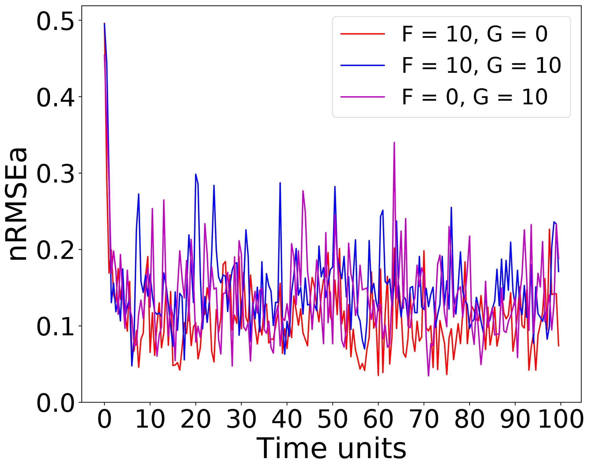
Figure 1 Time series of nRMSEa over the first 100 time units (2000 DA cycles) using $\mathit{\alpha }=\mathit{\gamma }=\mathrm{1}$ on $n/\mathrm{2}=\mathrm{18}$ grid points with an ensemble size of N=40 with the entire state vector observed at every time step.

The first connection between the filter performance and the model instabilities is drawn from Fig. 2 that shows the nRMSEa as a function of the number of the ensemble members. In line with previous findings for uncoupled univariate (Bocquet and Carrassi, 2017) and with coupled models (Tondeur et al., 2020), Fig. 2 shows that, even with a multivariate model, the error converges to very low values as soon as the ensemble size exceeds the number of unstable–neutral modes, n₀, and that it does not further decrease by adding more members. This behaviour is possible because error evolution is bounded to be linear or weakly non-linear. This means that one can in principle induce linearity intentionally in the error evolution to meet the aforementioned relation between filter accuracy and ensemble size and use it to infer the number of unstable–neutral modes. In a DA experiment, a “practical” way to achieve this is by strengthening the observational constraint (i.e. by increasing the measurements spatial and temporal density); here we observe the full system's state at every time step.

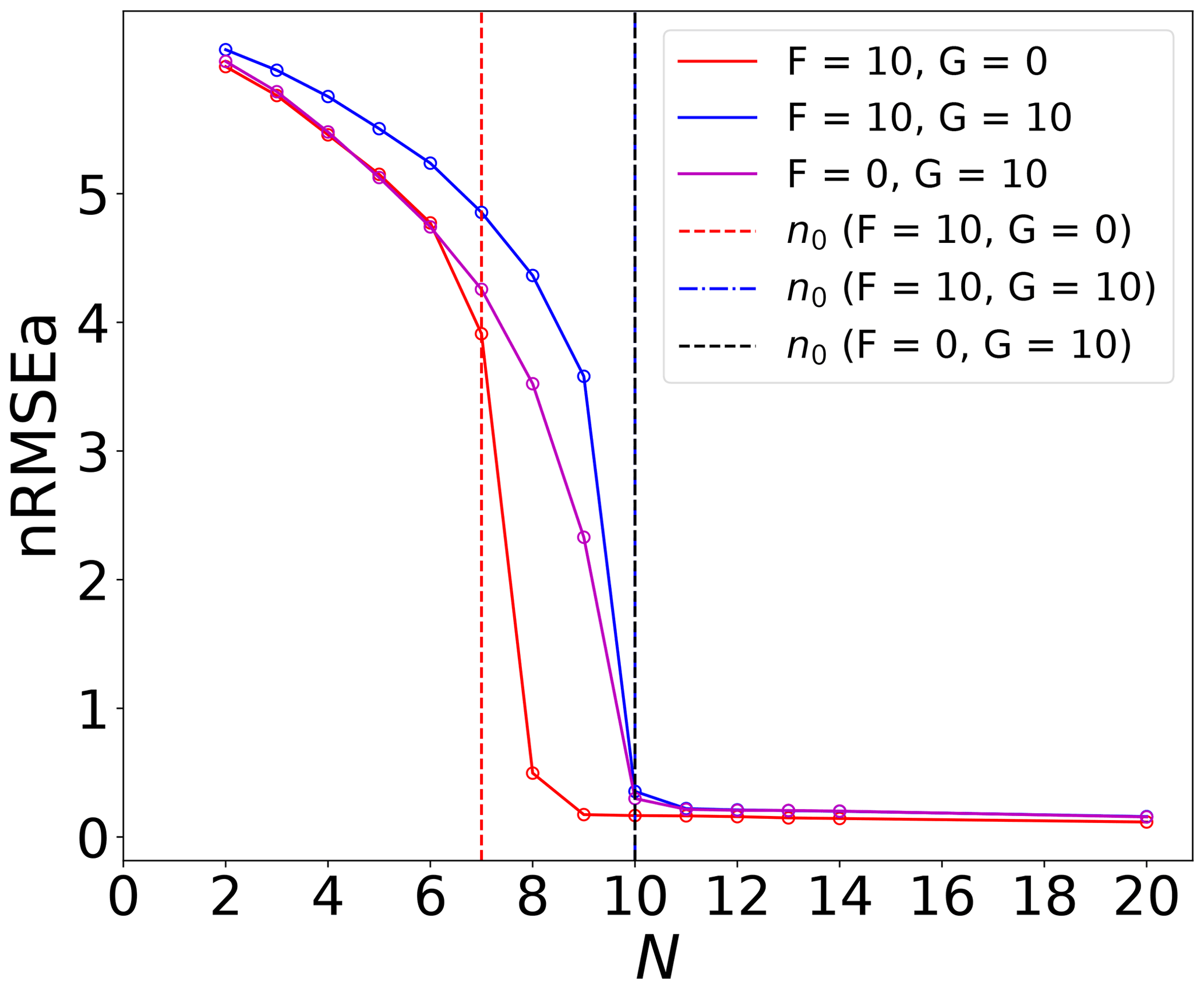
Figure 2 The time-averaged nRMSEa for all experiment configurations. The vertical dashed lines indicate the dimension of unstable–neutral subspace, n₀. The n₀ under the forcing $F=\mathrm{10},G=\mathrm{10}$ is the same as the forcing condition $F=\mathrm{0},G=\mathrm{10}$, which shows overlapped vertical lines. For the sake of numerical errors, the neutral mode is chosen as the LE that is closest to 0.

As mentioned above, the VL20 model represents four main physical mechanisms: (i) conversion between kinetic and potential energy, (ii) the energy injection from external forcing, (iii) the advection, and (iv) the dissipation. Although these processes all participate in the evolution of the model, the non-linear interplay cannot be straightforwardly disentangled. Nevertheless, we shall try to refer to them when interpreting the outcome of the DA experiments. In particular, in each experiment we will attempt to identify the prevailing mechanism over the aforementioned four. We perform three experiments, where we observe the full system state (i.e. H=I₃₆), or alternatively X or θ alone (implying in both cases $\mathbf{H}\in {\mathbb{R}}^{\mathrm{18}\times \mathrm{36}}$). Results are given in Fig. 3, that displays the time-averaged nRMSEa (global or for the dynamics or thermodynamics only) over a range of the coefficient α that modulates the energy transfer rate.

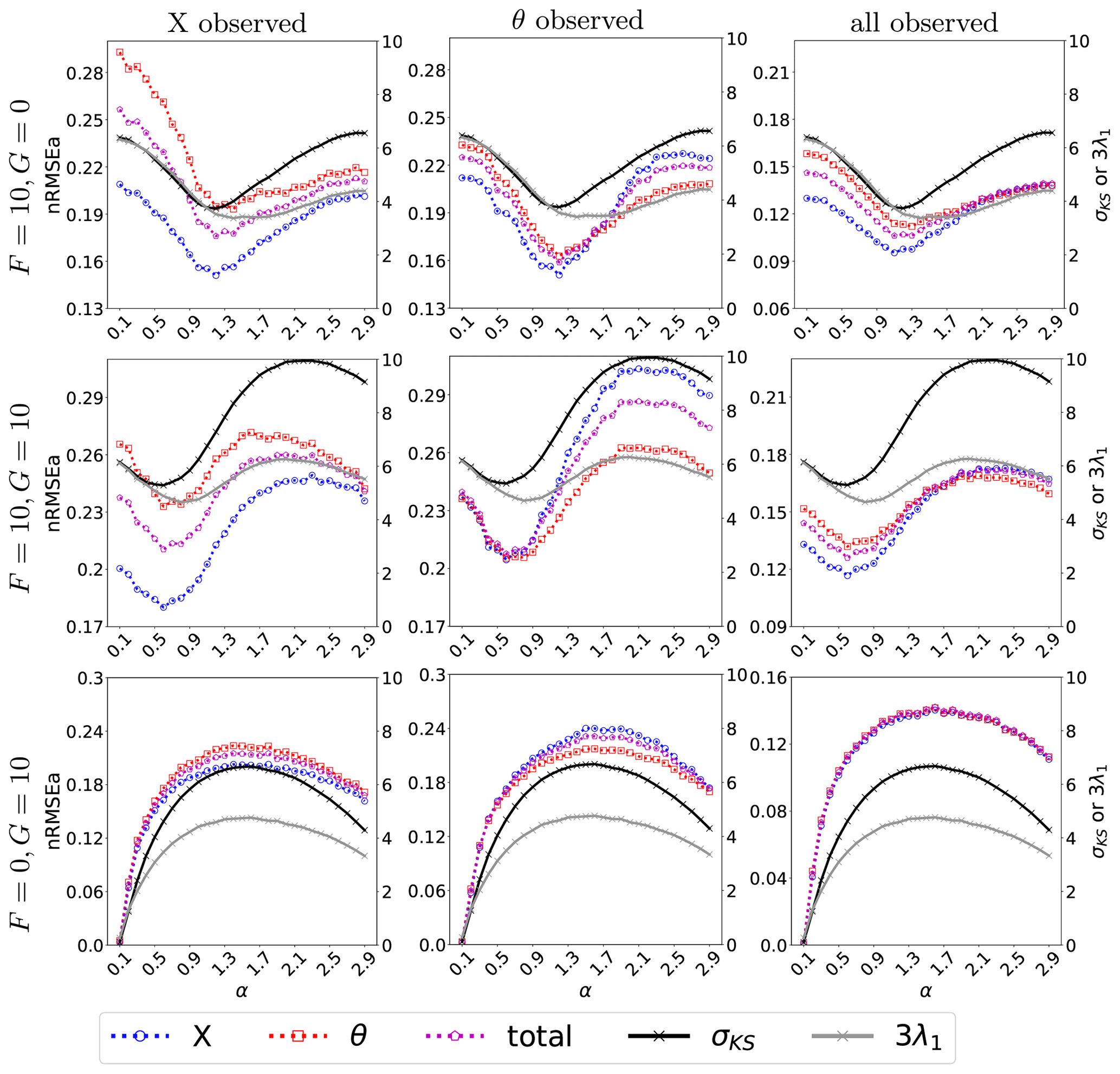
Figure 3 The nRMSEa with varying energy transfer coefficient $\mathit{\alpha }\in (\mathrm{0},\mathrm{3})$ (with an interval of 0.1) and dissipation coefficient γ=1. The left axis represents nRMSEa, while the right axis shows the σ_KS and the λ₁ (solid grey line) scaled by a factor of 3. The results come from perfect model assumption with observations at each time step where all variables, only X, or only θ is observed. The dashed blue line indicates the nRMSE of the X variable, the dashed red line represents the nRMSE of the θ variable, and the dashed purple line shows the nRMSE of the entire state vector.

Overall, and as expected, the analysis error is smaller in the observed variables (cf. the left and middle columns and corresponding colour lines) and attains the smallest level when X and θ are simultaneously observed (right column). Nevertheless, a few remarkable points can be raised. First, when the system is fully observed, for large values of α (i.e. for large conversion between available potential energy and kinetic energy) the skills in X and θ become very similar (right column): we conjecture this to be a consequence of the system getting more evenly turbulent with all variables sharing a similar internal variability as energy is exchanged efficiently between the kinetic and potential form. Second, for small values of α (i.e. small energy conversion), the effect of external forcing becomes dominant and determines the analysis error of X and θ (last column in Fig. 3). For instance, whenever the momentum is externally forced (F=10), the error in X is systematically smaller than in θ (first and second rows of the last column): DA is more effective in controlling the dynamics than the thermodynamics, even when they are subject to the same observational constraint. The situation is somehow reversed when only the thermodynamical variables are forced ($F=\mathrm{0},G=\mathrm{10}$): the analysis error of the momentum and the thermodynamic variable is undifferentiated. With small values of α and no forcing for the momentum, the non-linear momentum advection is limited by the small magnitude of the momentum that is not able to activate much the dynamical variables, so that we observe similar analysis error between the thermodynamics variable and the momentum.

Finally, the effect of the energy transfer and advection can be revealed by looking at the partially observed experiments (left and middle columns). Both mechanisms involve the momentum, making it more efficacious to observe X than θ, especially in the energy-transfer-dominated regime (large α). However, in an advection-dominated regime (small α), if θ is unobserved, X has limited capability to constrain the error in θ due to the weak feedback from θ to X. On the other hand, observing θ reduces error in X via the accurate estimate of the advection process of θ (see middle column).

Further insight into the role of the driving (unstable) variable and on the interplay between the prevailing physical mechanisms and the analysis error is given by looking at the CLVs (Kuptsov and Parlitz, 2012). In Fig. 4 we show at (normalized time-averaged) absolute amplitude of CLVs components along the state vector: it tells us which variable type/component has the larger influence on each CLV, thus indicating what processes participate more in a specific direction of error growth/decay.

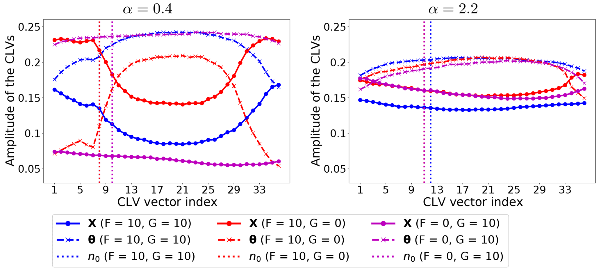
Figure 4 Normalized time-averaged amplitude of CLV components (the absolute value) for α=0.4 and α=2.2. In both cases γ=1. The vertical lines indicate the corresponding dimension of the unstable–neutral subspace, n₀.

As discussed above, changes in the value of α lead to shifting between the advection-dominated regime and an energy mixing one: these two regimes are portrayed in Fig. 4, by selecting α=0.4 and α=2.2. Moreover, these two values of α correspond roughly to those giving the largest differences in nRMSEa between the momentum and the thermodynamic variables (cf. left and middle panels of Fig. 3). For small energy exchange (α=0.4 – left column in Fig. 4), the model instabilities are driven by the external forcing, with the driving variable being the one where energy is injected. This is clearly visible when comparing the amplitudes of CLVs between X and θ in the left panel of Fig. 4: larger amplitudes of the unstable–neutral CLVs are found in the forced variables. When the momentum and the thermodynamics are equally forced (blue lines), the amplitude of the unstable–neutral CLVs for X and θ is close to each other. The non-linear advection process intensifies the error growth, especially for X. The non-linear advection and the momentum are of lesser importance if the momentum is not forced ($F=\mathrm{0},G=\mathrm{10}$ – purple lines), while the thermodynamic processes control both the stable and unstable subspace dominantly. The thermodynamic variable on the stable subspace acts as an energy sink to stabilize the dynamical system. The effect of the thermodynamics is shown noticeably by the large relative amplitude of the CLVs of the thermodynamic variable in the stable subspace when the momentum is directly forced (F=10 – blue and red line).

The behavior changes substantially when the energy exchange is the dominant physical mechanism (α=2.2 – right column). This causes a stronger mixing across the model variables so that both X and θ play a comparable role in the unstable–neutral components of the CLVs, leading to similar amplitude of the CLVs for all types of forcing. Remarkably, the effect of the energy conversion also applies to the stable components of the CLVs, leading to similar amplitude of the CLVs between X and θ.

The results in Fig. 4 reveal the effect of the prevailing physical mechanisms on determining the driving unstable variables. The figure suggests what variables should in principle be controlled by targeting measurements on the portion of the system's state vector with larger amplitude on the unstable–neutral CLVs.

Along with α, the energy in the system is modulated by the dissipation parameter, γ: larger values of γ imply an efficient removal of energy from the system, thus reducing the system's variability of both the potential and kinetic energy. At dynamical level, the parameter γ controls the contraction of the phase space as the sum of all Lyapunov exponents (equal to the average flow divergence) is −nγ. Hence, one expects that larger values of γ correspond to weaker instability for the model, as in the case of the classical L96 model (Gallavotti and Lucarini, 2014). Figure 5 is the same as Fig. 3 but for the dissipation, γ. Overall, we see that, with large γ, the system's internal variability reduces, and we find similar small errors in both X and θ. For weaker dissipation, the momentum is better controlled than the thermodynamics. With partial observations (left and middle columns), the error is much larger than in the corresponding fully observed cases. Similar to Fig. 3, the momentum is generally better reconstructed by the DA than the thermodynamics, although observing the latter appears more efficacious (i.e. it leads to smaller analysis error) than observing the momentum. We think that this is due to the prevailing mechanism being the advection of the thermodynamics given that α=1 in these experiments (cf. also Fig. 3). The amplitudes of the CLVs along the state vector are studied in Fig. 6. We consider the cases γ=0.4 and γ=1.0 for which the difference in the nRMSEa between X and θ is roughly the largest (cf. Fig. 5).

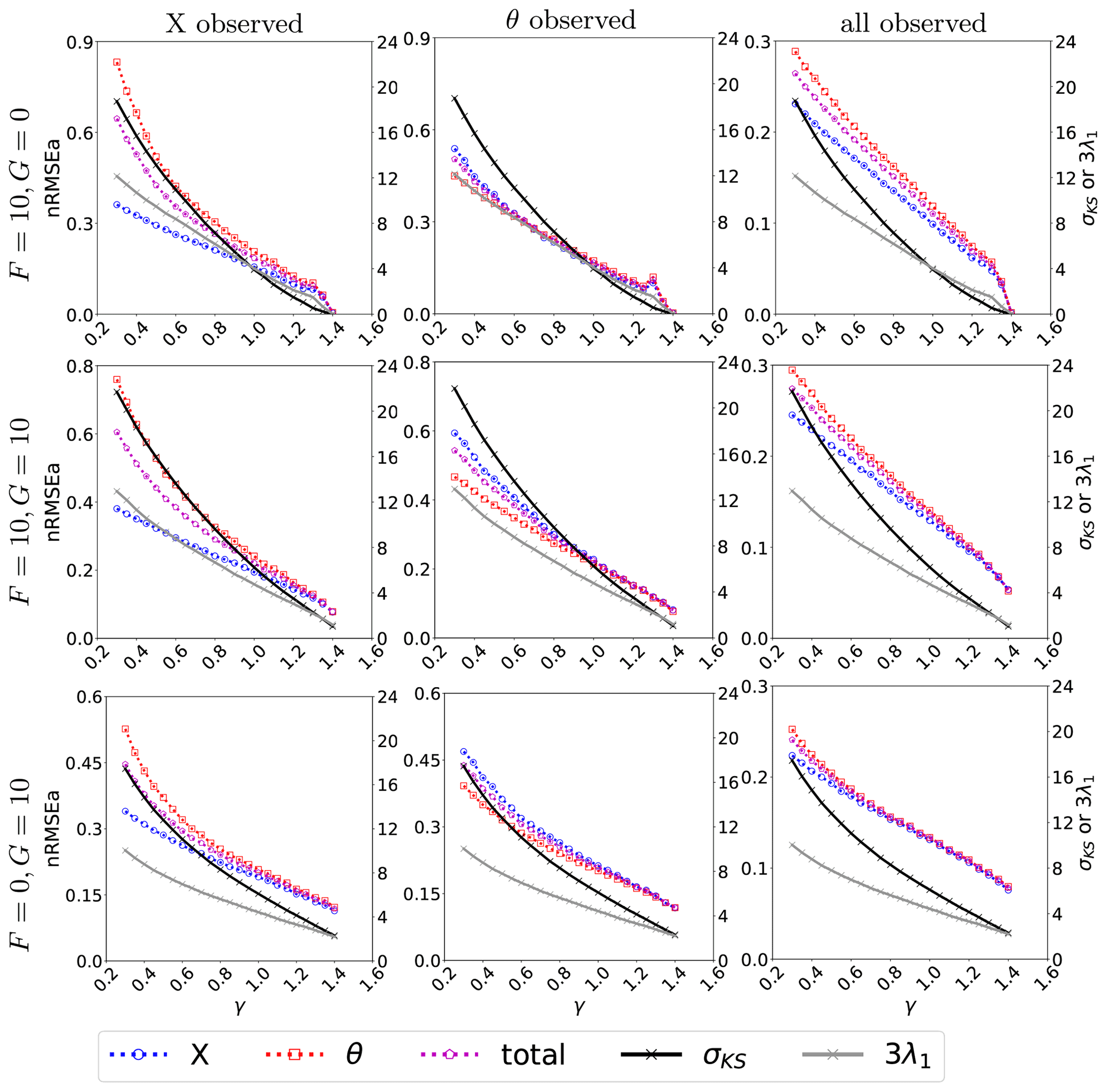
Figure 5 The nRMSEa with varying dissipation coefficients $\mathit{\gamma }\in [\mathrm{0.3},\mathrm{1.8})$ (with an interval of 0.05) and α=1. The left axis represents nRMSEa (dashed lines), while the right axis shows the σ_KS (solid black line) and the λ₁ (solid grey line) scaled by a factor of 3. The results come from perfect model assumption with observations at each time step where all variables, only X, or only θ is observed. The dashed blue line indicates the nRMSE of the X variable, the dashed red line represents the nRMSE of the θ variable, and the dashed purple line shows the nRMSE of the entire state vector.

Figure 6 Normalized time-averaged amplitude of CLV components for γ=0.4 and γ=1 with α=1. The vertical lines indicate the dimension of the unstable–neutral subspace.

With the leading CLVs strongly affected by the external forcing, the amplitude of the CLVs along the system's components is similar to the pattern of low energy exchange rate in Fig. 4 where α=0.4, even though here, α=1. This confirms that the dynamical regime of our experiments lies in the regime dominated by advection, and dissipation does not mix the kinetic and potential energy diffusely as the energy exchange, but rather it uniformly removes both types of energy without changing the prevailing physical mechanism. This is also reflected in the consistently low nRMSEa for the observed variable when varying dissipation rates in the partially observed experiments (see Fig. 5). The decreasing analysis error in Fig. 5 corresponds to the increases of γ, which reduces the dimension of the unstable–neutral subspace with increased relative importance of forced variables in the unstable–neutral subspace as the fast energy removal reduce the amount of energy mixing.

The results of Sect. 4.1 confirm the relation between the performance of DA (in terms of analysis error) and the dimension and characteristics of the unstable–neutral subspace. In particular, we conclude that successful DA relies on controlling the error in the unstable–neutral subspace by observing the variable that drives the error growth. The VL20 model enabled the investigation of the relation between the DA and the specific physical mechanisms such as the advection, the energy transfer among dynamics and thermodynamics, and the dissipation. The effect of DA (i.e. its efficacy) is strongly influenced by the form of the coupling between the unobserved and the observed variables that is in turn shaped by the prevailing physical mechanisms.

4.2 Inferring the degree of model instability with data assimilation

The derivation in Sect. 2 shows that, in the linear setting, the assimilation error is asymptotically bounded from above by a factor dependent on the observation error, the first LE and the number of unstable–neutral modes of the underlying forecast model. In this section we explore the extent to which this result holds in a non-linear scenario whereby the observational constraint is strong enough such that the error evolution is maintained approximately linear or weakly non-linear. We shall make use of numerical experiments with the VL20 model.

A first insight on the existence of a direct relation between the model instabilities and the skill of the EnKF-N is already provided in Figs. 3 and 5. They display the Kolmogorov–Sinai entropy, σ_KS (black line), and the first LE, λ₁ (amplified by a factor of 3 – grey line), along with the nRMSEa (discussed in Sect. 4.1). Even just by visual inspection, the figures clearly show the high correlation between the analysis error and both the σ_KS and λ₁.

The nature of this relation is further studied in Fig. 7, which shows scatter plots between the nRMSEa (with black markers) and ${\mathit{\sigma }}_{\text{KS}}/{\mathit{\lambda }}_{\mathrm{1}}$ in a log–log scale. Data points relative to experiments with forcing values are given in the panels' legends and with varying energy exchange and dissipation rates in the range $(\mathit{\alpha }\times \mathit{\gamma })\in [\mathrm{0.1},\mathrm{3})\times [\mathrm{0.3},\mathrm{1.8})$. Here, the EnKF-N assimilates the full state vector at each time step. The analysis error appears in a linear relationship with either σ_KS or λ₁, as long as $\ln \left(\text{nRMSEa}\right)\ge -\mathrm{4}$. The existence of such an approximate relationship provides the possibility to infer σ_KS and/or λ₁ based on the outcome of DA.

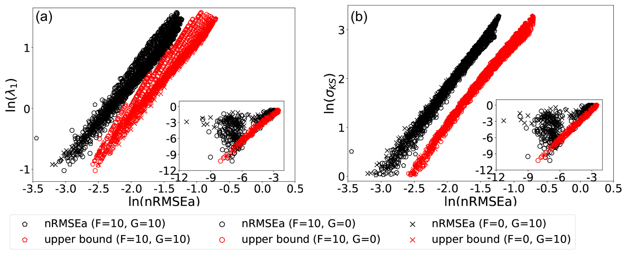
Figure 7 Scatter plots of λ₁ (a) and σ_KS (b) against the nRMSEa for experiments with observations of the entire state vector at each time step. The theoretical analysis error upper bounds are also displayed (red markers). The log scale is used on both axes. The experiments use the model forcing given in the legend and the energy rate and dissipation in the range $(\mathit{\alpha }\times \mathit{\gamma })\in [\mathrm{0.1},\mathrm{3})\times [\mathrm{0.3},\mathrm{1.8})$ with an interval of 0.1×0.05. The stable configurations (σ_KS≤0) have been excluded. The inset shows the weakly unstable model configurations ($\mathrm{0}<{\mathit{\sigma }}_{\text{KS}}\le \mathrm{1}$).

The scatter plots also demonstrate the validity of the upper bound (red markers) of Eq. (26) in Sect. 2. To compute the bound we set the coefficient related to observation, β=1, as it is compared to analysis errors normalized by observational error. The nRMSEa is bounded by the theoretical upper bounds for most of the model configurations considered. The linear relationship of the upper bound can be explained by its formulation in Eq. (26), where the exponent $e^{\mathrm{2}{\mathit{\lambda }}_{\mathrm{1}}\mathrm{\Delta }t}-\mathrm{1}$ can be approximated as 2λ₁Δt if 2λ₁Δt is sufficiently small. The spread of upper bounds points for given λ₁ values (left panel) reflects the various values of n₀ under similar λ₁ values. The better correspondence (narrower spread of the scattered points) in the plane nRMSEa with σ_KS (right panel) shows the importance of including both the dominant error growth rate, λ₁, and the unstable-subspace dimension, n₀, – both present in σ_KS – to better characterize the system's instabilities. The correspondence between σ_KS and the theoretical upper bound could also be a result of the relation between λ₁ and σ_KS as in a highly turbulent case, there is a linear relation between λ₁ and σ_KS (Gallavotti and Lucarini, 2014).

The linear relation does not hold for numerical experiments when $\ln \left(\text{nRMSEa}\right)<-\mathrm{4}$ (see the black markers' distribution in the panels' inset). We explain this behaviour in the following way. The wide clouds of points correspond to all model configurations with very small σ_KS and λ₁. In these quasi-stable dynamics, the error growth in between successive analysis is very little, with occasional error decay. The observational error, which is random and white in time, will be often larger than the forecast error and will dominate the analysis error, thus breaking its direct dependence on the instability-driven forecast error. In addition, in the weakly unstable model configurations, the most unstable direction behaves almost like a neutral mode, which also breaks the assumptions of the theoretical upper bound for unstable models. In fact, we do not show the weakly unstable results with σ_KS<1 for both σ_KS and λ₁.

The error bounds in Sect. 2 rely on the assumption of linear error evolution, a condition that we met in our experiments thanks to a strong observational constraint, with (synthetic) measurements covering the full state vector at each time step. These conditions are rarely achievable in practice, so it is relevant to explore how results will change with a lighter observational constraint. There are three direct ways to achieve this by acting on (i) the number/type of measurements, (ii) the measurement error, and/or (iii) the temporal frequency.

The effect of the first is studied in Fig. 8 that is similar to Fig. 7 but for DA experiments whereby only one of each variable in the VL20 is observed.

Figure 8 Scatter of σ_KS (a) and λ₁ (b) against nRMSEa for experiments where either the momentum or the thermodynamic variable alone is observed. The log–log scale is used on both axes, and points represent experiments with the same model parameter values used in Figs. 3 and 5, excluding weakly unstable cases with σ_KS<1 and hence excluding cases where $\ln \left(\text{nRMSEa}\right)<-\mathrm{4}$, similar to Fig. 7.

The impact of partially observing the system causes the emergence of a weakly quadratic relationship between the analysis error and either σ_KS or λ₁. However, the analysis error is still uniquely and monotonically related to them, especially for σ_KS. A quadratic law requires one additional coefficient to be determined compared to a linear law; yet the mere existence of such a law suggests again that one could in principle infer σ_KS and/or λ₁ based on the analysis error. With the relaxed observation constraint, the analysis error can (and indeed do so in several instances) exceed the theoretical upper bound. However, the general trend of the numerical experiments still follows the theoretical upper bound.

We study the effect of changing the amplitude of the observational error in Fig. 9. Results reveal that varying the observation error in the range of 5 %–10 % does not break the quasi-linear relationship between the analysis error and σ_KS or λ₁. The nRMSEa is quite insensitive to the observation variance due to the normalization. Nevertheless, the upper bound limit is not violated as in Fig. 7, and the slope of the nRMSEa from the numerical experiment is remarkably similar to the slope of the theoretical bound.

Figure 9 Scatter plots of σ_KS (a) and λ₁ (b) against nRMSEa. The log–log scale is used on both axes. The different points refer to experiments with different observation error given in the legend and model parameter as in Figs. 3 and 5, excluding weakly unstable cases with σ_KS<1 and hence excluding cases where $\ln \left(\text{nRMSEa}\right)<-\mathrm{4}$, similar to Fig. 7.

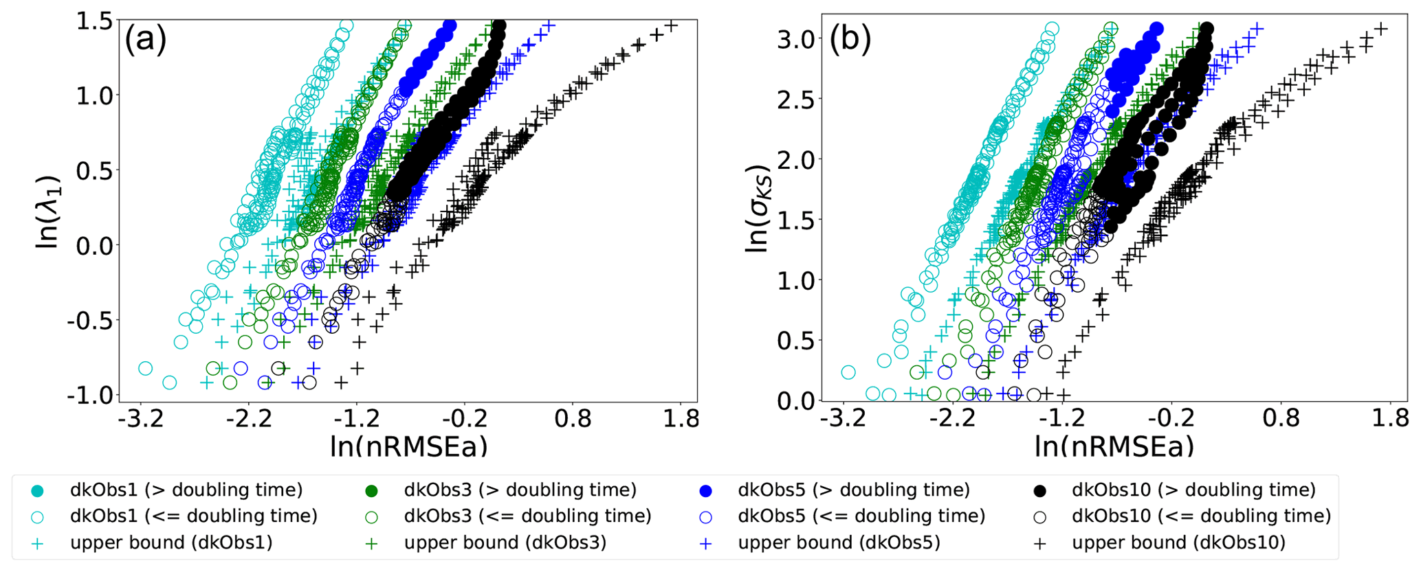
Figure 10 Scatter plots of σ_KS (a) and λ₁ (b) against nRMSEa. The log–log scale is used on both axes. The different points refer to experiments with different observation intervals given in the legend and model parameters as in Figs. 3 and 5, excluding cases when σ_KS<1. The filled circle represents the cases where the observation interval exceeds the doubling time of the error.

Finally, the impact of varying the observation frequency is explored in Fig. 10. It is patent that decreasing the frequency leads to blurring the linear relation between the analysis error and the σ_KS or λ₁. There is a clear deviation from the trend of the theoretical upper bound and from the uniqueness of the relation between analysis error and σ_KS, as soon as the observational time interval exceeds the error doubling time (that is inverse related to λ₁), and DA error evolves beyond the linear regime. However, for frequent enough observations, a linear relation similar to the upper bound appears, and, again, one could in principle deduce σ_KS and/or λ₁ based on DA.

The larger sensitivity to the observation frequency than to observation noise (cf. Figs. 9 and 10) is a direct consequence of the different effects these two factors have in determining the degree of non-linearity of the error. This is explained, for the L96 model, in the Appendix of Bocquet and Carrassi (2017) using a dimensional analysis. The key point is that the observation frequency modulates directly the magnitude of the non-linear term in the model, namely the advection. Decreasing the observation noise, while effectively reducing the analysis error, is not sufficient to keep the error dynamics linear if Δt>0 and the model is chaotic.

5 Conclusions

It is sometimes of great importance to be able to obtain information on the instability of a system of interest by performing data analysis of suitably defined observables. This is of key importance when one does not have direct access to the evolution equations of the system or when the analysis of its tangent space is too computationally burdensome. As an example, quantitative information on the degree of instability of a chaotic system can be extracted using extreme value theory by studying the statistics of close dynamical recurrences as well as of extremes of so-called physical observables (Lucarini et al., 2014, 2016). The use of such a strategy has shown great potential for the analysis of geophysical fluid dynamical models in a highly turbulent regime (Gálfi et al., 2017) as well for the understanding of the properties of the actual atmosphere (Faranda et al., 2017; Messori et al., 2017).

In this study, we have addressed this problem by taking the angle of DA. The relation between DA and the instability of the dynamical system where it is applied has long been studied (see, for example, Miller et al., 1994; Carrassi et al., 2008), and has been used to design DA techniques in various field of geosciences (Carrassi et al., 2022; Albarakati et al., 2021). Here, we have reversed this viewpoint and investigated the possibility of using DA to infer fundamental quantities of the underlying dynamics, in particular the Lyapunov exponents, λ_i, or the Kolmogorov–Sinai entropy (σ_KS). The basic idea is to look at DA as a control problem and relate our ability to control the system, ceteris paribus, to its underlying instability. We have leveraged a stream of previous works that set the theoretical foundation and that proved the convergence of the error covariance of the Kalman filters onto the unstable–neutral subspace of the dynamical system. Based on this, we derived here an upper bound of the Kalman filter forecast error, i.e. under the assumptions of a linear model dynamics and a linear observation operator. The upper bound is very informative as it relates the error's amplitude to all of the essential descriptors of the model instabilities on the one hand and of the DA on the other. These are the dimensions of the unstable–neutral subspace, n₀, the first Lyapunov exponent, λ₁, the frequency of the observation assimilation, Δt, and the observation error, β_k. By properly normalizing the bound by the observation error, it can be written as a function of the model dynamical properties exclusively.

The existence of a relation between λ₁ or σ_KS and the DA skill, as well as the validity of the bound, has then been investigated in a non-linear scenario using numerical experiments. We have used the EnKF-N (Bocquet et al., 2015) as a prototype of deterministic EnKF (Evensen, 2009) and the new model developed by Vissio and Lucarini (2020). The VL20 is an extension of the widely used Lorenz 96 model that includes a thermodynamic component. While maintaining all of the virtues of a low-dimensional model suitable for investigations on new methods at low computational cost, VL20 is conceptually much richer than the original L96 model. In particular it allows for the exchange of energy between a kinetic and potential form, which, together with forcing and dissipation, provides the fundamental framework for the Lorenz (1955) energy cycle. Additionally, as advection impacts temperature-like variables, one can observe the emergence of more complex dynamical behaviours. By changing the value of its key parameters, and in particular of those determining its forcing and dissipation, the model explores various dynamical regimes, ranging from fixed point, periodic, quasi-periodic, and chaotic behaviour. In terms of DA, the VL20 model has the attractive feature that it includes two qualitatively different set of variables, associated with dynamics and thermodynamics, respectively. Hence, it is possible to explore the problem of having partial observation beyond focusing of the spatial extent of the observations only.

We demonstrate that the skill of the EnKF-N is directly linked to both λ₁ and σ_KS. Whenever the error within the EnKF-N cycles is kept sufficiently linear via a strong observational constraint, the relation is clearly linear too. By relaxing the observational constraint (by either reducing the frequency of measurements or by increasing their noise), deviation from linearity emerges. Nevertheless, the linear relation is very robust against the level of observational noise (within certain range), while it turns quadratic once the interval between successive measurements gets too large and it exceeds the system's doubling time. Similarly, we found out that the theoretical upper bounds for the errors, derived for a linear system, still hold, as long as the observational constraint is strong enough, but are then violated.

The error bound and the linear/quasi-linear relation between the error and λ₁ or σ_KS represent two direct ways to infer λ₁ and σ_KS by looking at the output of a DA exercise. First, we can use the bound (Eq. 26) to estimate λ₁ for a specific dynamical model, based on (normalized) error output of a DA exercise. This requires the unstable–neutral subspace dimension, n₀, that can be obtained, in the case of EnKF-like methods, by looking at the analysis error convergence for increasing ensemble size; N: n₀ will be equal to $N^{*}-\mathrm{1}$, where N^* is the smallest ensemble size for which the error reaches its minimum. This procedure will give us an underestimate of λ₁. Nevertheless, our results (cf. Fig. 7) seem to suggest that the amount of the underestimation is small and, notably, constant across a range of different model configurations (and thus possibly quantifiable).

Our numerical experiments indicate a second way to estimate λ₁ or σ_KS from the skill of DA. The linear/quasi-linear relationship between normalized DA error and λ₁ or σ_KS (cf. Fig. 7) exists for both the derived upper bound in Eq. (26) and numerical experiments and is tested under various observation constraints. The existence of the relationship for the upper bound implies that the relationship may exist for other dynamical systems as long as the time between analysis Δt is sufficiently frequent because the upper bound is based on the assumption of a (quasi-)linear model. To utilize the relationship for a specific dynamical system, a few DA experiments using different set of parameters of the dynamical system are required. A linear relation can be obtained by linear regression from the selected data, by which a relatively accurate λ₁ or σ_KS for other parameters of the dynamical system can be inferred. Unavoidably, for the selected set of parameters, the method requires the λ₁ or σ_KS to be known, which possibly can be obtained by computational methods such as the one proposed by Wolfe and Samelson (2007). However, the resulting linear relation can lead to a computationally efficient approach for other sets of parameters of the dynamical system with an estimate more accurate than the one from the upper bound in Eq. (26).

The linear relation between error and λ₁ and σ_KS will certainly be more complicated with model errors. From Grudzien et al. (2018a) and Grudzien et al. (2018b), we know that the KF error covariance will no longer be fully confined within the unstable–neutral subspace but could maintain projections everywhere and thus also on the stable modes. Those projections would be asymptotically zero in the absence of model noise. While this remains to be investigated, we argue that the existence of a clear monotonic relationship between analysis error and λ₁ will still hold in the presence of model error. The relation to σ_KS might also still stand because the correction would come from weakly stable modes. However, the conjecture needs to be validated by numerical experiments that are outside of the scope of this paper.

We are currently considering how these results will change when performing DA for state and parameter estimation. In this context, a relevant recent study has shown how the minimum number of ensemble members, N^*, will need to be increased to include as many members as the number of parameters to be estimated (Bocquet et al., 2020). By modifying its parameters, the model's instabilities' properties will change too, potentially inducing a catastrophic change (a tipping point) in its long-term behaviour. Data assimilation will then need to infer the best parameter values to track the data signal and keep the DA solution in the same region of the bifurcation diagram.