the Creative Commons Attribution 4.0 License.
the Creative Commons Attribution 4.0 License.
 | 14 Oct 2021
Identification of linear response functions from arbitrary perturbation experiments in the presence of noise – Part 2: Application to the land carbon cycle in the MPI Earth System Model
Guilherme L. Torres Mendonça
Julia Pongratz
Christian H. Reick
The response function identification method introduced in the first part of this study is applied here to investigate the land carbon cycle in the Max Planck Institute for Meteorology Earth System Model. We identify from standard C4MIP 1 % experiments the linear response functions that generalize the land carbon sensitivities β and γ. The identification of these generalized sensitivities is shown to be robust by demonstrating their predictive power when applied to experiments not used for their identification. The linear regime for which the generalized framework is valid is estimated, and approaches to improve the quality of the results are proposed. For the generalized γ sensitivity, the response is found to be linear for temperature perturbations until at least 6 K. When this sensitivity is identified from a 2×CO2 experiment instead of the 1 % experiment, its predictive power improves, indicating an enhancement in the quality of the identification. For the generalized β sensitivity, the linear regime is found to extend up to CO2 perturbations of 100 ppm. We find that nonlinearities in the β response arise mainly from the nonlinear relationship between net primary production and CO2. By taking as forcing the resulting net primary production instead of CO2, the response is approximately linear until CO2 perturbations of about 850 ppm. Taking net primary production as forcing also substantially improves the spectral resolution of the generalized β sensitivity. For the best recovery of this sensitivity, we find a spectrum of internal timescales with two peaks, at 4 and 100 years. Robustness of this result is demonstrated by two independent tests. We find that the two-peak spectrum can be explained by the different characteristic timescales of functionally different elements of the land carbon cycle. The peak at 4 years results from the collective response of carbon pools whose dynamics is governed by fast processes, namely pools representing living vegetation tissues (leaves, fine roots, sugars, and starches) and associated litter. The peak at 100 years results from the collective response of pools whose dynamics is determined by slow processes, namely the pools that represent the wood in stem and coarse roots, the associated litter, and the soil carbon (humus). Analysis of the response functions that characterize these two groups of pools shows that the pools with fast dynamics dominate the land carbon response only for times below 2 years. For times above 25 years the response is completely determined by the pools with slow dynamics. From 100 years onwards only the humus pool contributes to the land carbon response.
- Article
(3305 KB) - Full-text XML
- Companion paper
- BibTeX
- EndNote


In Part 1 of this study (Torres Mendonca et al., 2021a) we developed a method to identify linear response functions from arbitrary perturbation experiments. The RFI method (response function identification method) was tested by means of artificial toy model simulations. Here, we demonstrate the applicability of our method to a practical problem: we investigate the dynamics of the land carbon cycle in the Max Planck Institute for Meteorology Earth System Model (MPI-ESM; see Appendix A). In particular, we show how our RFI method provides insight into two aspects of central relevance to carbon cycle research: the sensitivity of the land carbon cycle to changes in atmospheric CO2 and its distribution of internal timescales.
The global carbon cycle plays a critical role in mitigating climatic effects from CO2 emissions. According to the yearly published Global Carbon Budget (Friedlingstein et al., 2020), the ocean and land components of this cycle have taken up about half of the anthropogenic CO2 emitted from pre-industrial times to 2019. Despite its relevance to climate, the dynamics of the carbon cycle is still poorly understood (Ilyina and Friedlingstein, 2016). Improving our understanding of this dynamics, in particular in response to CO2 perturbations, is therefore one of the major challenges of climate research (Marotzke et al., 2017).
A tool long employed to investigate the carbon cycle dynamics are linear response functions. Such functions have been used to predict atmospheric CO2 from emissions (Bolin et al., 1981; Siegenthaler and Oeschger, 1978; Oeschger and Heimann, 1983; Maier-Reimer and Hasselmann, 1987; Enting, 1990; Joos et al., 1996; Joos and Bruno, 1996), land carbon storage from NPP (net primary production) (Bolin et al., 1981; Thompson and Randerson, 1999) and GPP (gross primary production) (Emanuel et al., 1981), and to disentangle the historical development of the land and ocean carbon sinks from ice core reconstructions of atmospheric 12CO2 and 13CO2 (Joos and Bruno, 1998). Linear response functions have also been employed to study the dependence of global warming on possible future CO2 emissions and the associated GWP (global warming potential) (Caldeira and Kasting, 1993; Joos et al., 2013; Caldeira and Myhrvold, 2013; Ricke and Caldeira, 2014; Gasser et al., 2017).
However, a generally underexplored field in carbon and also climate research is that of internal timescales (see however Todd-Brown et al., 2013; Friend et al., 2014; Koven et al., 2015; He et al., 2016). Also here, linear response functions open an interesting perspective. To systematically investigate the interaction between climate and the carbon cycle, for more than a decade now internationally coordinated simulation exercises have been performed with several Earth system models within the Coupled Climate Carbon Cycle Model Intercomparison Project (C4MIP; see Fung et al., 2000; Friedlingstein et al., 2006) that today belongs to the international Coupled Model Intercomparison Project (CMIP; see Taylor et al., 2012). With every round of CMIP, quite some effort is put into understanding how differences in simulation results from the participating Earth system models arise (see, e.g., Anav et al., 2013; Tebaldi et al., 2021; Arora et al., 2020). It is pretty clear that parts of the differences arise from different spectra of internal timescales. These differences show up, e.g., in the standard 4×CO2 and 1 % experiments of the CMIP protocol that are explicitly designed to estimate equilibrium and transient climate sensitivity (Taylor et al., 2012; Eyring et al., 2016). However, such a characterization of the response of temperature to radiative forcing by only two numbers is rather incomplete: these numbers are the aggregated result of system responses at all its internal timescales together. Therefore, a more detailed insight into system behavior could be obtained from the knowledge of this spectrum of responses at different timescales. Such insight may be provided by considering the linear response function that generalizes climate sensitivity (e.g., Ragone et al., 2016). Further, this perspective to obtain from linear response functions information on internal timescales is not restricted to climate sensitivity, but also applies to other types of system characteristics like the airborne fraction (e.g., Le Quéré et al., 2009; Raupach, 2013), the TCRE (Transient Climate Response to Cumulated Emissions; see e.g., Ciais et al., 2013) and the β and γ sensitivities introduced by Friedlingstein et al. (2003) to characterize how land and ocean carbon react to rising CO2 and rising temperatures. In the present study we explore the application of linear response functions to study β and γ. In particular, we focus on the β and γ values that characterize the land carbon cycle, whose response presents already for several C4MIP rounds a large model spread (Friedlingstein et al., 2006; Arora et al., 2013, 2020).
When studying the land carbon response, the γ value quantifies the sensitivity of the land carbon cycle to the radiative effect of CO2 acting via greenhouse warming, while the β value quantifies its sensitivity to the biogeochemical effect of CO2 concentrations on photosynthetic carbon assimilation (Arora et al., 2013, 2020; Schwinger et al., 2014; Adloff et al., 2018). Mathematically, γ is defined as the ratio between changes in the land carbon caused by the radiative effect of CO2 (ΔCrad) and changes in temperature (ΔT) at a particular time:
β is defined as the ratio between changes in the land carbon caused by the biogeochemical effect of CO2 (ΔCbgc) and changes in atmospheric CO2 concentration (ΔCatm) at a particular time:
However, although these two values give insight into the magnitude of the sensitivities, they cannot be seen as properties of the land carbon cycle alone. The reason is that γ and β quantify the sensitivity of land carbon to CO2 perturbations only for a particular perturbation scenario, so that for different scenarios one may obtain different values (Gregory et al., 2009; Arora et al., 2013).
To quantify this sensitivity in a more systematic way and thereby gain deeper insight into the land carbon dynamics one needs a more general formalism. For small changes in atmospheric CO2 one can show that by accounting for the memory of the carbon cycle these values generalize to linear response functions, which turn out to be properties of the land carbon cycle itself (Rubino et al., 2016; Enting and Clisby, 2019, see also Appendix B). As a result, these linear response functions characterize the land carbon sensitivities for any perturbation scenario. For this reason these functions will here be called land carbon generalized sensitivities.
The essential step to investigate the carbon cycle dynamics within this general formalism is the identification of the generalized sensitivities. Typically, the γ and β values proposed by Friedlingstein et al. (2003) are obtained taking data from standardized C4MIP simulation experiments where, starting from an equilibrium state, atmospheric CO2 concentration is increased by 1 % each year (e.g., Gregory et al., 2009; Arora et al., 2013, 2020; Schwinger et al., 2014; Adloff et al., 2018; Williams et al., 2019). Since data from such 1 % experiments performed with C4MIP models are readily available in international databases, one would be interested in identifying the generalized γ and β sensitivities as well from these experiments. However, methods in the literature to identify response functions from data require special perturbation experiments, and C4MIP experiments were not tailored for this purpose. It is here that our RFI method is useful. Our method is designed to derive response functions from experiments driven by any arbitrary perturbation. Thus, in the present study we show that by this method one can robustly derive the land carbon generalized sensitivities for the MPI-ESM taking data from standard C4MIP 1 % experiments. To make sure the identified generalized sensitivities are indeed characteristics of the land carbon cycle in the MPI-ESM, we demonstrate their predictive power by applying them to predict the response of the model in several experiments that were not used for their identification. In preparation for future studies applying these generalized sensitivities to study the dynamics of the carbon climate system in C4MIP models, we also investigate various ideas to improve the quality of the recovery of the response functions by using additional types of data routinely available in C4MIP simulations or using log-transformed data to account at least partially for process-immanent nonlinearities that hinder the usage of experiment data from larger levels of forcing.
Apart from giving a systematic quantification of the sensitivities, as hinted above linear response functions can be a powerful tool to gain insight into the internal dynamics of the carbon cycle. Because response functions fully characterize the linear response of a system, they contain information on its distribution of internal timescales, i.e., the weights with which characteristic timescales from internal processes contribute to the macroscopic response of the system. These weights may shed light into which are the most relevant processes to the response at different timescales. For our application to the land carbon, such information may give insight into the main processes influencing the model spread found in the C4MIP results.
However, while several studies have tried to obtain the weights of different timescales in the carbon cycle by fitting response functions to a sum of a few exponents (Maier-Reimer and Hasselmann, 1987; Enting and Mansbridge, 1987; Enting, 1990; Joos et al., 1996, 2013; Pongratz et al., 2011; Colbourn et al., 2015; Lord et al., 2016), in principle it is not clear to what extent such results can be trusted, let alone interpreted. The reason is that finding these weights from data is a severely ill-posed problem that requires special methods to be dealt with (Istratov and Vyvenko, 1999). In contrast to the classical fitting procedures, by employing a regularization technique (Groetsch, 1984; Engl et al., 1996) combined with a novel estimation of the noise level in the data (see Part 1) our RFI method accounts for this ill-posedness. In addition, instead of assuming that the response functions result from only few timescales, the RFI method recovers a continuous spectrum of timescales, in agreement with what one would expect when studying the carbon cycle response (Forney and Rothman, 2012a). In the present work we show that, in contrast to results obtained with classical fitting procedures, spectra recovered by the RFI method may be reliable and even interpretable. For this purpose, we investigate a relatively detailed spectrum of timescales that arises from a high-quality recovery of the generalized β sensitivity. We examine (i) the robustness of the obtained spectrum and (ii) the explanation for its timescale structure.
An additional novelty introduced here is a simple procedure to estimate the linear regime of the response, i.e., the range of perturbation strengths for which the response of the system can be considered linear. As discussed in Part 1, the presence of traces of nonlinear responses in the data can severely deteriorate the recovery of the response function. Hence, to make sure that the data from which the response function is recovered contain no strong nonlinearities, one must be able to estimate the linear regime of the response. Because the response functions will be derived from 1 % experiments, we introduce a technique to estimate with the aid of additional simulations the linear regime from this type of experiment. By this technique the linear regime of the response of land carbon to changes in CO2 and climate for the MPI-ESM will be estimated.
The outline of the paper is as follows. In the next section we introduce the methodology of the study including the RFI method, the C4MIP experiments, and the technique to estimate the linear regime of the response from “percent” experiments. In Sects. 3 and 4 we identify and investigate the generalization of the γ and β sensitivities in the MPI-ESM. In Sect. 5 we investigate the detailed spectrum of timescales obtained for the generalized β sensitivity. In Sect. 6 the results are summarized and discussed.
In this section we introduce the methodology employed throughout the study. We start by briefly introducing the RFI method (for a detailed description please refer to Part 1), the C4MIP-type experiments considered here, and technical details for the identification of the generalized sensitivities. Then, we present our procedure to estimate the linear regime of the response from “percent” experiments.
2.1 RFI method and C4MIP experiments
The RFI method identifies the response function χ(t) taking data from the response Y(t) – in our example the global land carbon – and the perturbation f(t) – atmospheric CO2 or temperature (see below) – assuming the following relation (see Part 1):
where η(t) is a noise term. Here ΔY(t) and Δf(t) mean that we are taking only the change in the variables with respect to their equilibrium values from a control simulation. Following Forney and Rothman (2012a), the spectrum of internal timescales is obtained by assuming that the response function χ(t) can be represented by an overlay of exponential modes:
To account for the large range of timescales in the carbon cycle (Ciais et al., 2013) it is useful to rewrite Eq. (4) in terms of log 10τ, so that
The spectrum of timescales is then given by q(τ), which following the terminology from Part 1 we call simply spectrum. The problem is solved by discretizing Eqs. (3) and (5), prescribing a distribution of timescales τ, taking the data on ΔY(t) and Δf(t), and solving a minimization procedure for the spectrum q(τ). The parameters to prescribe the distribution of timescales are taken identically to those chosen for the application to the toy model in Part 1. To treat the ill-posedness we employ Tikhonov–Phillips regularization (Phillips, 1962; Tikhonov, 1963) in a singular value decomposition (SVD) framework that gives the solution by the expansion (Hansen, 2010; Bertero, 1989)
where • is the usual scalar product, M is the number of timescales, ui and vi are the singular vectors, σi are the singular values, λ is the regularization parameter, and fi(λ) are the filter functions
The regularization parameter λ is determined by the discrepancy method (Morozov, 1966) with noise level estimated from a SVD analysis of the data combined with information from the control simulation. Once the spectrum qλ is found, the response function χ(t) follows from Eq. (5).
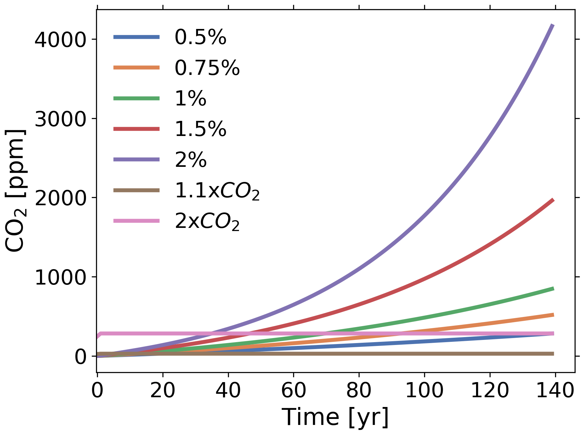
All linear response functions are identified by the RFI method taking data from C4MIP-type experiments performed with the MPI-ESM. We focus on identifying the response functions from standard 1 % experiments that are widely available in international databases. In addition, to examine the quality of the results, we also identify some response functions taking data from additional experiments. To investigate the robustness of the identified response functions, we employ them to predict the response of the MPI-ESM in several experiments not used for the identification. A summary of the experiments considered in the study is given in Table 1, with forcing scenarios shown in Fig. 1.
The variables taken for the identification of the response functions are the ones relevant for the quantification of the land carbon sensitivities γ and β, respectively:
- (a)
the change in global land carbon in response to changes in global land temperature;
- (b)
the change in global land carbon in response to changes in atmospheric CO2.
Global land carbon is computed as the sum of the total land carbon over all grid cells of the model. Global land temperature is calculated as the mean near-surface air temperature over land at 2 m height. The changes are computed as , with YPI being the mean value of observable Y from a control simulation at pre-industrial conditions. Since the main interest lies in long-term variations, annual mean data are used.
As demonstrated in Appendix C, the generalization of the β sensitivity can be shown to be monotonic. Therefore, in the following we will derive it employing the additional noise-level adjustment in the RFI algorithm (step 6 of Fig. 1 in Part 1). Since the generalization of the γ sensitivity is not known to be monotonic, for this sensitivity the RFI algorithm will be applied without the additional adjustment.
Table 1C4MIP-type experiments considered in this study. Forcings are shown in Fig. 1. Abbreviations “rad” and “bgc” refer to standard CMIP model setups used to calculate the climate-carbon cycle sensitivities. In the “rad” (radiatively coupled) setup only the radiation code of the model is affected by changes in atmospheric CO2. This setup is used to calculate γ. In the “bgc” (biogeochemically coupled) setup only the biogeochemistry of the model is affected by changes in atmospheric CO2. This setup is used to calculate β. In brackets are names of standard CMIP experiments.

2.2 Estimating the linear regime from “percent” experiments
As described in Part 1, the recovery of response functions is complicated by the presence of noise and nonlinearities. The RFI method is designed to cope with the former. In the present section we present a technique to cope with the latter, but at the expense of performing additional response experiments. This technique will serve as a complement to the RFI method in the application to the land carbon cycle in the following sections. By these additional experiments we will determine the range of forcing strengths for which the response can be considered linear – an analysis in general not possible using only the control and perturbation experiments on which the RFI method is based.
Before we introduce this technique to cope with nonlinearities, it is useful to specify more clearly what we mean by “nonlinearity”. Dynamical systems like the Earth system are crowded with nonlinearities. Our notion of “nonlinearity” is much more specific: the linear response formula (Eq. 3) can be interpreted as the linear term in a Volterra expansion of the response ΔY(t) of the system into the perturbation Δf(t) (see Sect. 2 in Part 1). This expansion is given by
where 𝒪((Δf)2) represents terms of order 2 and higher in the perturbation Δf. For small enough perturbations the term 𝒪((Δf)2) is small compared to the linear-order term and can be ignored, so that Eq. (8) yields Eq. (3). Throughout this study, nonlinearities are defined as the nonlinear terms 𝒪((Δf)2) in this expansion. Indeed, these nonlinear terms arise from the intrinsic nonlinearities of the underlying system. In the language of statistical mechanics one would call those intrinsic nonlinearities as “microscopic”. This in mind, our notions of linearity and nonlinearity should then be termed “macroscopic”. Since the idea here is to study the linear response of the system, we will be interested only in the case where perturbations are so small that the nonlinear terms 𝒪((Δf)2) can be ignored. However, the question is whether they can be ignored. It is clear that nonlinearities may gain importance with increasing forcing strength. Hence, to study only the linear response, experiment data can be used for our purpose only up to such perturbation strengths where nonlinearity start to contribute to the response; i.e., we have to identify the regime where the response is still linear. This is the purpose of the technique that we describe in the following.
To introduce our technique we use the example of simulations with the linear toy model employed in Part 1. To demonstrate the effect of nonlinearities on the recovery of χ(t), following Part 1 we artificially add a nonlinear term −aY2(t) to the linear response Y(t) of the toy model:
In this way we obtain a nonlinear response Ynonlin(t), with nonlinearity strength controlled by the parameter a, from which χ(t) is derived. In addition to including this nonlinear term in the toy model response, to introduce the technique we will need to quantify the quality of the recovery of the response function. Since in our application to the land carbon the “true” response function is not known a priori, following Part 1 we quantify the quality of the recovery indirectly by measuring the quality with which the recovered response function can predict the response of the model in experiments not used for the recovery itself. For this purpose we introduce the relative prediction error
where ⋆ stands for the convolution operation, ΔYk and Δfk are the response and the perturbation in experiment “k”, and χ is the response function recovered from the 1 % experiment.
We can now present our technique. Taking first a purely linear situation (a=0), we show in Fig. 2a the relative prediction error (Eq. 10) when using the response function obtained from a 1 % simulation to predict the response from two other % simulations with smaller growth rate. More precisely, performing a sequence of 1 % experiments for increasingly longer simulation periods, we calculated for each experiment the response function and used it to predict the response for a 0.5 % and 0.75 % experiment covering the same simulation period. Then we plotted in Fig. 2a the relative prediction error against the final forcing strength of the 1 % experiment. As a result, it is seen that with increasing final forcing strength the relative prediction error decreases. This happens because in this linear case the SNR is increasing with increasing simulation period, i.e., with increasing final forcing strength, so that the recovery of the response function continuously improves.
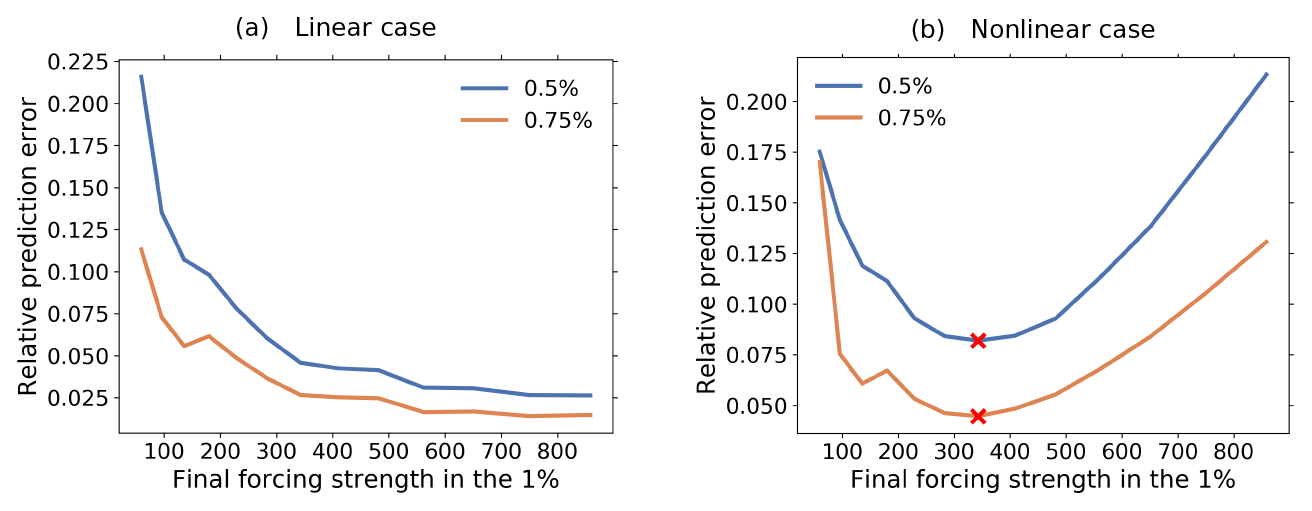
Figure 2Toy model example for the identification of the linear regime by using additional experiments. Shown is the relative prediction error (Eq. 10) for the response of 0.5 % and 0.75 % experiments as obtained from the response function calculated by the RFI method from 1 % experiments. The relative prediction errors are plotted against the final forcing strengths of a sequence of 1 % experiments with increasing time series length. The crosses at the minima indicate the final forcing strength for which the response function is optimally recovered (see text). (a) shows the behavior for the fully linear toy model (a=0) and (b) the behavior in the presence of nonlinear contributions to the response (). For the purpose of demonstrating more clearly the increase in the relative prediction error for a decrease in the forcing strength, we include in the plot cases where the forcing strength is extremely small, corresponding to very small time series lengths. To deal with such cases, we set for a number of data points N<30 the number of timescales M=N (see parameters for the RFI method in Part 1). For such small number of timescales, usually no plateau in the singular values spectrum is found (step 2 of Fig. 1 in Part 1). Therefore, for these special cases we also modify the algorithm to interpret the two smallest singular values as a plateau, since their small magnitude makes them have a similar effect to those singular values belonging to the plateau itself. In addition, to illustrate the most general case where χ(t) is not known to be monotonic, we exclude here the monotonicity check (step 6 of Fig. 1 in Part 1).
Calculating the relative prediction error only for experiments with smaller growth rate becomes important in the next case where nonlinearities are considered (Fig. 2b). This plot was obtained by the same procedure except that we took for the nonlinearity parameter a value a>0. As seen, in this nonlinear case the relative prediction error is first improving but deteriorating afterwards. For small forcing, nonlinearities are small and therefore the relative prediction error behaves as in the linear case; i.e., it decreases with final forcing strength. However, when forcing strengths become larger, nonlinearities start to contribute substantially to the response, thereby causing a deterioration of the recovery of the response function and consequently the relative prediction error once more increases. This increase of the prediction error can be unambiguously traced back to the presence of nonlinearities in the 1 % simulation because the prediction error was calculated only for experiments with smaller growth rate, i.e., smaller forcing strength throughout the whole simulation. Therefore, nonlinearities contribute already substantially to the response in the 1 % simulation before they become relevant in the other experiments. Accordingly, with this type of experiment setup we can be sure that the increase in the prediction error comes solely from the deterioration of the recovery of the response function and not from nonlinearities in the additional experiments used for calculating the prediction error.
Obviously, for forcing strengths smaller than at the minimum, nonlinearities do not hinder the recovery of the response function, so that one can consider this to be the regime of linear system behavior. In view of the trade-off between noise and nonlinearities, for the 1 % experiment the response function is thus optimally recovered when taking as final forcing strength the value at the minimum of the prediction error curve. Similarly, if the error curve has no minimum (as in the linear case shown in Fig. 2a), the optimal recovery is obtained from the experiment with the largest forcing strength.
With the presentation of this additional technique to identify the linear regime we are ready for the application to the MPI-ESM in the next sections.
In this section we identify from MPI-ESM simulations the linear response function χγ (generalized γ sensitivity), defined by
where now the response is ΔY(t):=ΔCrad(t) and the forcing is Δf(t):=ΔT(t), with ΔCrad(t) being the change in global land carbon obtained in the “rad” experiment (see Table 1) and ΔT(t) the change in global land temperature.
That χγ indeed generalizes γ can be understood by considering that γ is defined by
for a negligible noise η(t). From Eq. (12) it is clear that by knowing χγ(t) one can compute the response ΔCrad(t) and thereby γ(t) for any time-dependent perturbation ΔT(t), as long as the perturbation strength is small. Hence, χγ(t) can be seen as a property of the land carbon system and a generalization of γ(t).
3.1 Estimating the linear regime
As a first step in obtaining a proper approximation of χγ(t), we investigate what maximum forcing strength can be used to ensure that the recovered χγ(t) is not spoiled by the presence of nonlinearities. Using the technique introduced in Sect. 2.2, we show in Fig. 3 the relative prediction error (Eq. 10) for χγ(t) recovered from the 1 % rad experiment as a function of the final forcing strength in the 1 % rad experiment. There is no clear minimum, so that for the data available the recovery of χγ(t) seems not to be limited by nonlinearities. For optimal recovery we thus take the full time series, i.e., the maximum final forcing strength.
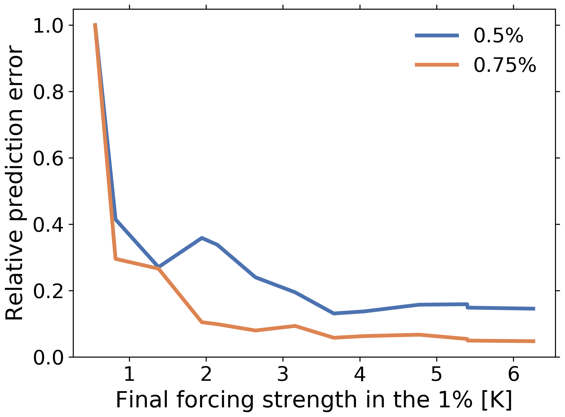
Figure 3Relative prediction error (Eq. 10) for the 0.5 % and 0.75 % rad experiments using χγ(t) recovered from the 1 % rad experiment. The error is shown as function of the final forcing strength used for the recovery of χγ(t). No clear minimum is found, so that the recovery seems not to be limited by nonlinearities.
3.2 χγ and the quality of its recovery
The quality of the recovery can in principle be improved by taking an experiment with better SNR. To investigate whether the recovery from the 1 % rad experiment can be further improved, we also applied the RFI algorithm to recover χγ from the 2×CO2 rad experiment. We chose the 2×CO2 rad experiment because as shown in Fig. 4 it has smaller forcing strengths than the maximum forcing strength for the 1 % rad experiment – therefore nonlinearities should also not limit the recovery – but is expected to carry useful information over a larger range of the response spectrum. This expectation can be justified as follows (MacMartin and Kravitz, 2016). Taking the Laplace transform of Eq. (11) gives
where the tilde denotes Laplace transformed functions. From Fig. 4 it is seen that for the 1 % rad experiment the temperature ΔT behaves approximately as a linear function, which gives a Laplace transform proportional to . For the 2×CO2 rad experiment, the temperature behaves approximately as a step function (ignoring the transient in the first 20 years), which gives a Laplace transform proportional to . This means that for the same χγ, the first term on the right-hand side of Eq. (13) – the “clean” response – decays to zero faster for the 1 % rad experiment than for the 2×CO2 rad experiment. Hence, assuming the same noise η for both cases, the response from the 2×CO2 rad experiment is buried in the noise only at larger p, meaning that this experiment carries useful information until higher rate values p than the response from the 1 % rad experiment.

The response function χγ(t) recovered from the two types of experiments is shown in Fig. 5a. As expected, the different experiments indeed result in different recoveries. Because we know from the analysis of Fig. 3 that nonlinearities do not limit the recovery, the difference between the two response functions probably results from the difference in the quality of the data from the two types of experiments. To compare the robustness of each recovery, we analyze how well they predict the response from other experiments (Fig. 5b and c). If the response function is correctly recovered, it should be able to predict not only experiments with smaller, but also experiments with higher forcing rates. Therefore, we also include in the analysis 1.5 % and 2 % rad experiments. To exclude errors that may be caused by nonlinearity, we take as a conservative estimate of the linear regime forcing strengths smaller than the final forcing strength at the end of the 1 % rad experiment (which is approximately the maximum forcing strength; see temperature value at t=140 years for the 1 % rad experiment in Fig. 4). We take these values as an estimate of the linear regime because the 1 % rad experiment has only 140 years, so that no estimate for higher forcing strengths is available. Hence, for the 1.5 % and 2 % rad experiments the responses are expected to be reasonably predictable at least until the values marked with circles, where their respective forcing strengths reach this maximum forcing strength. All other experiments have forcing strengths smaller or equal to this maximum forcing strength, so that they should be predictable for the whole time series.
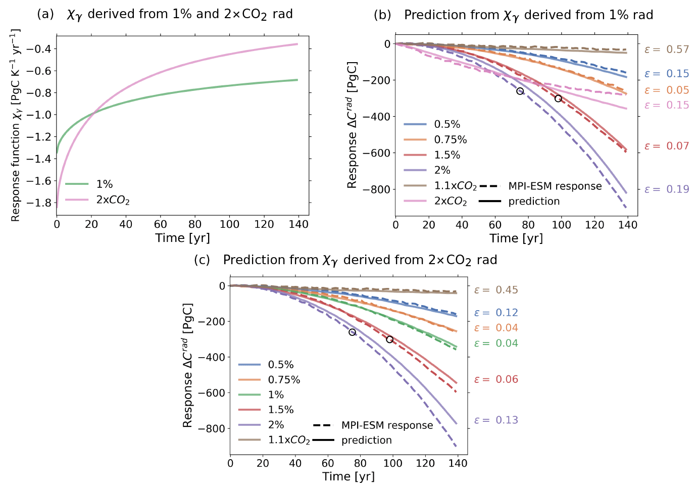
Figure 5χγ recovered from 1 % and 2×CO2 rad experiments (a) and prediction of model responses using these recoveries of χγ. Circles indicate the maximum value for which 1.5 % and 2 % responses are predictable according to the estimate of the linear regime (see text). At the right of (b, c) the relative prediction error (see Eq. 10) is indicated for the different experiments, calculated for the 1.5 % and 2 % rad experiments by considering only values preceding the circles.
Figure 5b shows the quality of the prediction using χγ(t) recovered from the 1 % rad experiment. Visually, model response and prediction seem to have a comparable quality of agreement across the 1.1×CO2, 0.5 %, 0.75 % and 1.5 % rad experiments, while for the 2 % and 2×CO2 rad experiments there are larger discrepancies. For a quantitative analysis, we compute for the estimated linear regime the relative prediction error (Eq. 10) for each experiment (right side of the plot). It is seen that the error varies from less than 10 % for the 0.75 % and 1.5 % rad experiments to values between 10 % and 20 % for the 0.5 %, 2 % and 2×CO2 rad experiments, and a significantly larger value of 57 % for the 1.1×CO2 rad experiment. To better understand these differences, it is important to note that as long as nonlinearities are small, experiments with higher forcing strength are expected to have smaller prediction error because they have higher SNR. This can be made plausible by considering that a perfectly recovered response function predicts a “clean” linear response (infinite SNR) with zero error, whereas the same response function can predict a noisy response only with some finite error. Therefore, if χγ(t) is well recovered, we expect large prediction errors for experiments with small forcing strengths such as the 1.1×CO2 rad – which is indeed the case – but small errors for experiments with large forcing strengths but still well within the linear regime such as the 2×CO2 rad (compare the forcing strengths for the 2×CO2 rad experiment and the maximum forcing strength for the 1 % rad experiment in Fig. 4). Since contrarily to the expectation the prediction error is not particularly small for the 2×CO2 rad experiment, probably the recovery of χγ(t) derived from the 1 % rad experiment is not completely accurate and may still be further improved. As suggested above, such improvement may be achieved by taking data with better quality from the 2×CO2 rad experiment.
Figure 5c shows the quality of the prediction using χγ(t) recovered from the 2×CO2 rad experiment. As expected, results indicate an improvement in the recovery (compare to Fig. 5b). The prediction error decreases for all experiments present in both plots. In addition, it also decreases if we compare the prediction of the 1 % rad response in Fig. 5c with that of the 2×CO2 rad response in Fig. 5b.
This section therefore suggests two main conclusions: first, for χγ(t) the response seems to be approximately linear for temperature perturbations up to at least 6 K. Second, the overall improvement of the prediction in Fig. 5c compared to Fig. 5b confirms the expectation from the Laplace transform analysis that the step-like 2×CO2 rad experiment indeed carries more information on the response function than the 1 % rad experiment. This suggests that step-like experiments may be more appropriate than the standard 1 % experiment for the identification of linear response functions.
In this section we identify the linear response function χβ (generalized β sensitivity), defined by
where now the response is ΔY(t):=ΔCbgc(t) and the forcing is Δf(t):=ΔCatm(t), with ΔCbgc(t) being the change in global land carbon found in the “bgc” experiment and ΔCatm(t) the change in atmospheric CO2 (and not atmospheric carbon content, as might be expected from the notation).
That χβ indeed generalizes β can be understood analogously to Sect. 3 by considering that β is defined by
for a negligible noise η(t). Hence, χβ(t) can be seen as a generalization of β(t) and a property of the land carbon cycle that characterizes the response ΔCbgc(t) to any time-dependent perturbation ΔCatm(t), as long as the perturbation strength is small.
4.1 Approaches to identify χβ
Similarly to the last section, we identify χβ(t) by several approaches to find the one that gives results with the best quality. For this purpose, we also consider in addition to Eq. (14) alternative formulas to derive χβ(t), each taking a different forcing. The identification is performed in three different ways:
-
Using CO2 as forcing (see Eq. 14);
-
Using the logarithm of CO2 as forcing:
where now the forcing is
with being the pre-industrial value for atmospheric CO2;
-
Using net primary production (NPP) as forcing:
The first approach is the same used throughout the paper: χβ(t) is identified using the ΔCatm(t) forcing from Eq. (14).
The second and third approaches are motivated as follows. In the “bgc” setup, changes of atmospheric CO2 affect land carbon exclusively via the resulting changes in primary productivity1. Therefore, the reaction of land carbon to CO2 perturbations may be understood as a two-step process: first, CO2 affects primary productivity (carbon assimilation); second, the assimilated carbon adds to land carbon storage. This second step is in models typically described by an almost linear system of storage compartment forced by NPP (see, e.g., Xia et al., 2013; Huang et al., 2018). Thus, presumably the response of land carbon to NPP is well described by a linear response function. These considerations underlie the second and third approaches but are more explicitly realized in the latter: there we first derive the linear response function χNPP(t) describing the response of land carbon to changes in NPP, and then use the data of the simulated dependence of NPP on CO2 to derive the desired response function χβ(t) (see Eq. 21). In this way we try to keep the most critical step in the identification of the response function, namely the inversion of the response integral, largely free from nonlinearities, and indeed, for this reduced problem, without much interference from nonlinearity we can recover the response function from experiment data obtained for much higher perturbation strengths than in the first approach, and because of the higher SNR the quality of recovery is thereby largely improved (see below). Instead of NPP one could also try to split off the nonlinear part by taking GPP (gross primary production), which differs from NPP only by the autotrophic respiration. However, autotrophic respiration is lost to the atmosphere, so that it is NPP and not GPP that adds to land carbon storage. Thus, by taking NPP instead of GPP the linear part is arguably splitted off more completely. The second approach is motivated in the same way, except that the nonlinear part is guessed to be a logarithmic function of CO2 as suggested by the Keeling formula (see, e.g., Alexandrov et al., 2003), so that here no additional NPP data are needed from simulations.
Mathematically, our procedure in each approach is the following. In the second approach (see Eq. 16), we employ as forcing a logarithmic expression because it is known that a large part of the nonlinear relation between CO2 and carbon storage comes from the approximately logarithmic dependence of NPP on CO2 (e.g., Alexandrov et al., 2003). Such formula has the advantage that the expansion of the forcing in Catm gives
Taking ΔCatm sufficiently small and comparing the result to Eq. (14) thus yields
Accordingly, the response function from Eq. (16) also gives the desired χβ(t).
In the third approach, we take directly the response to NPP (see Eq. 17). Expanding the forcing ΔNPP(Catm) in Catm gives
Taking ΔCatm sufficiently small and comparing the result to Eq. (14) yields
Accordingly, by this approach we compute χβ(t) in three steps: first, we identify the response function χNPP(t) using Eq. (17); second, we take the first derivative of NPP with respect to CO2 at ; third, we apply Eq. (21) to obtain χβ(t) from χNPP(t).
4.2 Checking nonlinearities with the three approaches
Before analyzing the recovery of χβ(t) employing the three approaches, one must verify that these two additional approaches indeed account for some of the nonlinearities in the response. If this is true, response formulas (Eqs. 16 and 17) should be able to predict the response to larger perturbation strengths than Eq. (14). To verify this expectation, in the following we compare the relative prediction error (Eq. 10) by applying Eqs. (14), (16) and (17).
Figure 6a shows the relative prediction error for χβ(t) recovered from the 1 % bgc experiment with the first approach (Eq. 14). The prediction is also computed via Eq. (14). The clear minima indicate the presence of strong nonlinearities for forcing strengths above around 100 ppm (94 ppm for the 0.5 % and 133 ppm for the 0.75 %). Therefore, in contrast to the case of χγ discussed in the last section, we see here that one indeed has to cope with the additional difficulty of nonlinearities.
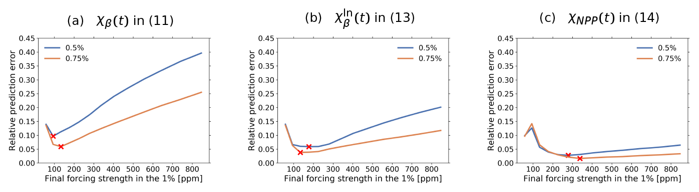
Figure 6Relative prediction error (Eq. 10) for the 0.5 % and 0.75 % bgc experiments obtained when using χβ(t), and χNPP(t) obtained from the 1 % bgc experiment to predict the response. The error is shown as a function of the CO2 final forcing strength.
Figure 6b shows the prediction error when using recovered from the 1 % bgc experiment with the second approach (Eq. 16). To check how well nonlinearities are accounted for by taking the logarithmic forcing, the prediction is also computed via Eq. (16). Compared to Fig. 6a, we see a slight improvement in the results: the minima have smaller prediction errors and the prediction errors increase at a slower rate for increasing final forcing strength. This indicates that using the logarithm of CO2 as forcing indeed accounts for some of the nonlinearities in the response. Accordingly, one can make predictions with smaller error for larger forcing strengths using Eq. (16) instead of Eq. (14).
Figure 6c shows the prediction error for χNPP(t) recovered via Eq. (17) from the 1 % bgc experiment (first step of the third approach). To check how well nonlinearities are accounted for by taking the NPP forcing, we also employ Eq. (17) for the prediction. Here, we see a substantial improvement in the results. The response is almost completely linear, with very “flat” minima. This indicates that a large part of the nonlinearity encountered in the response of the land carbon to changes in CO2 can indeed be explained by the nonlinear relationship between NPP and CO2. Accordingly, by employing Eq. (17) instead of Eq. (14) one can predict the response of the land carbon until forcing strengths as high as 800 ppm with an error smaller than 10 %.
4.3 χβ and the quality of its recovery
So far, we have only considered the ability of Eqs. (14), (16) and (17) to predict the land carbon response. Now, we analyze how well the generalized sensitivity χβ(t) can be identified by the three approaches. For the identification we took data from the 1 % bgc experiment until the CO2 forcing strength reaches the first minimum for each case in Fig. 6: ΔCatm=94 ppm for the first approach (30 years); ΔCatm=133 ppm for the second approach (40 years); and ΔCatm=279 ppm for the third approach (70 years). Since ΔCatm=279 ppm is approximately the forcing strength for the 2×CO2 bgc experiment and results from last section suggested that this type of experiment may carry more information for the identification, we employ the third approach, also taking the 2×CO2 bgc experiment. For the present application where the recovery is limited by nonlinearities, taking the 2×CO2 bgc experiment has the additional advantage that because its forcing strength has a constant value throughout the whole experiment, we can use the full time series (140 years). To compute the first derivative of NPP with respect to CO2 (second step of the third approach), we fitted the function NPP=NPP(Catm) to polynomials of order 4, 5, and 6 and then took the first derivative from the fits.
The results from the three approaches are shown in Fig. 7a. At short timescales there is an overall agreement among all recoveries with only small discrepancies. To be able to compare the results also for longer timescales, we extend the response functions recovered from the 1 % bgc experiment – obtained from time series with 30, 40, and 70 years, respectively, for the first, second, and third approaches – until 140 years (extensions are indicated by dotted lines). This can be done because with the RFI method we derive the response function from the ansatz (5), which formally gives the values of the response function for all times. The result is that all response functions recovered from the 1 % bgc experiment present relatively small discrepancies even at long timescales. Response functions derived from the 2×CO2 bgc experiment with the third approach show a similar behavior among themselves but differ from the recoveries using the 1 % bgc experiment. The reason for this difference will be investigated below.
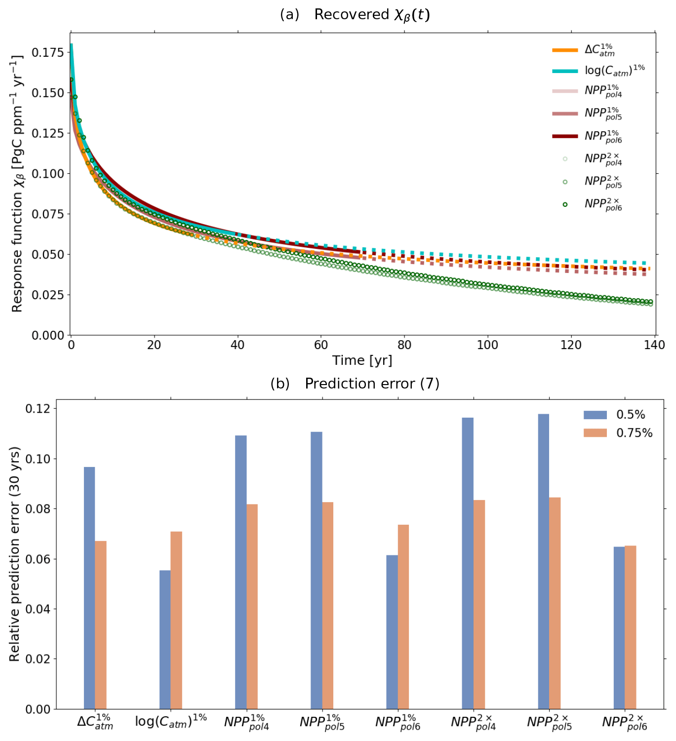
Figure 7Response function χβ(t) derived by the three approaches (a) and the respective prediction errors for the first 30 years of the response (b). : recovery with first approach from 1 % bgc experiment; log (Catm)1 %: recovery with second approach from the 1 % bgc experiment; : recovery with third approach from the 1 % bgc experiment using for the derivative a polynomial fit of order x; : recovery with third approach from the 2×CO2 bgc experiment using for the derivative a polynomial fit of order x. Continuous lines denote values of χ(t) that are within the time series length used for the recovery (30 years for , 40 years for log (Catm)1 % and 70 years for ). Dotted lines denote extended parts of the response function, i.e., values not covered by the time series used for the recovery but obtained from the recovered spectrum using Eq. (5). Circles denote the response functions derived taking the full time series (). For more details, see text.
To quantitatively compare the quality of the recoveries, we plotted in Fig. 7b the relative prediction error (Eq. 10). Since the response functions were derived using different time series lengths, for a fair comparison we compute the error only at the minimal time series length of 30 years (the time series length used for the first approach). Results show no large discrepancies among the different approaches. For the third approach, there seems to be a small advantage in using a polynomial of order 6 for the computation of the derivative.
However, results from Fig. 7b reflect only the quality of the recoveries at short timescales, for which anyway no large discrepancies were encountered in Fig. 7a. To evaluate the quality of the recovery also at long timescales, one must take the extended version of the response functions that were derived from shorter time series. Since the only substantial difference at long timescales in Fig. 7a is found between the response functions recovered from the 1 % and 2×CO2 bgc experiments, we take for this analysis exemplarily only the response functions recovered with the first approach (1 % bgc experiment) and the third approach (2×CO2 bgc experiment). By choosing the response function recovered with the first approach, we evaluate for the worst case scenario (where only 30 years are used for the recovery) how reliable predictions are for timescales longer than the time series used for recovery. In contrast, by choosing the response function recovered with the third approach from the 2×CO2 bgc experiment, we check whether the different values at long timescales are actually an improvement in the recovery. As mentioned above, such improvement is expected because this response function was recovered taking the full time series (140 years).
Following the same procedure as in the last section, in Fig. 8 we show the quality of the prediction for different experiments using the aforementioned recoveries of χβ(t). Figure 8a shows the results for the predictions calculated via Eq. (14) using χβ(t) recovered with the first approach. We take as an estimate of the linear regime forcing strengths smaller than the forcing strength at the first minimum in Fig. 6a. The response values corresponding to this forcing strength are marked in Fig. 8a with circles. It is seen that although χβ(t) was recovered using a time series of only 30 years, it predicts the 1.1×CO2 bgc experiment with only 3 % error over 140 years. Other experiments are predicted within the linear regime with error smaller than 10 % with exception of the 2 % bgc experiment, for which the error is around 14 %. Since the 2×CO2 has a constant forcing strength outside the linear regime already from the beginning, its prediction fails as expected for the whole time series.
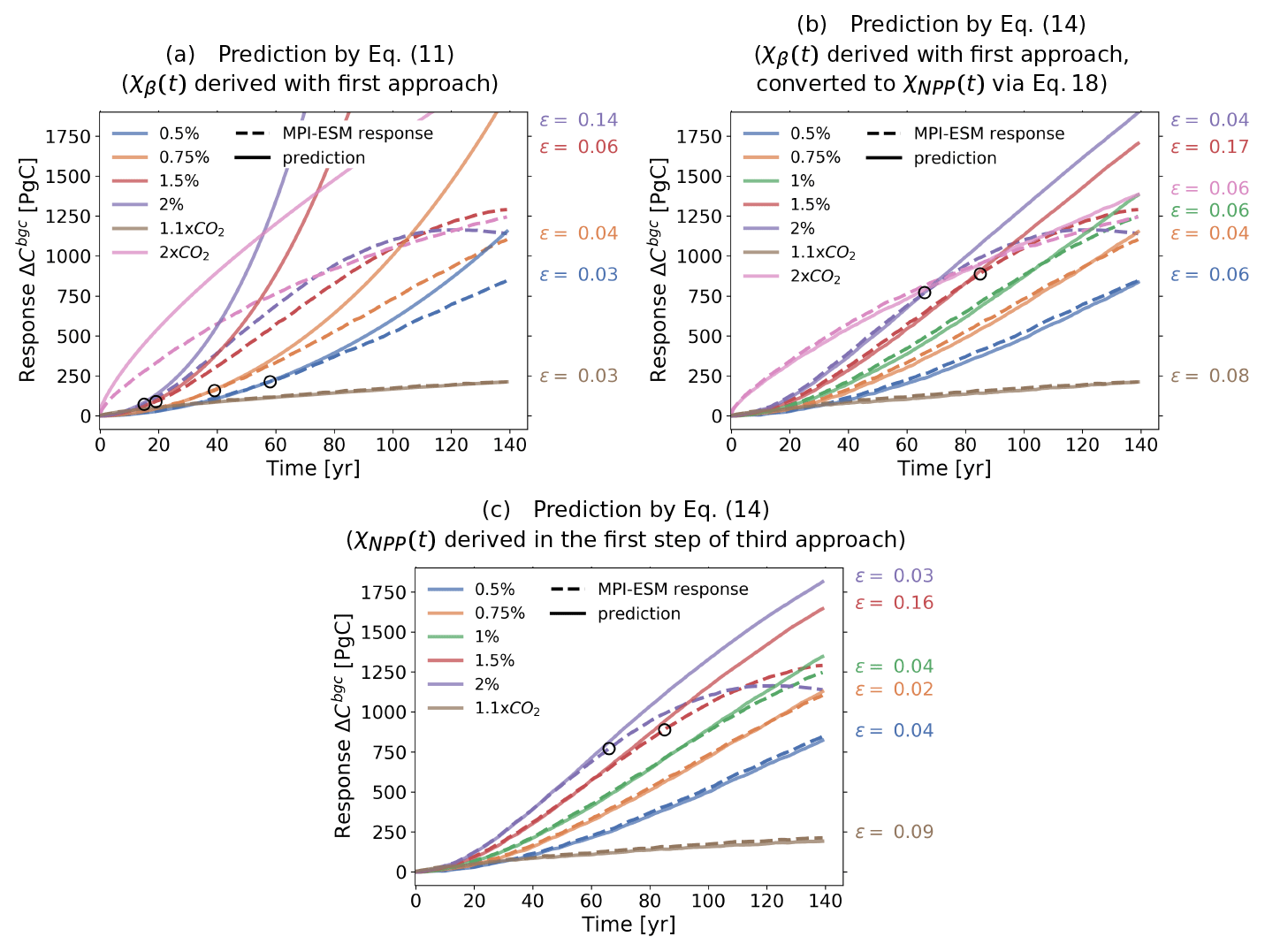
Figure 8Prediction of model responses employing response functions derived with the first approach from the 1 % bgc experiment (derived from data with 30 years length, but extended to 140 years) and with the third approach from the 2×CO2 bgc experiment (derived from data with 140 years length). (a) Prediction by Eq. (14) taking the response function χβ(t) derived from the 1 % bgc experiment with the first approach. (b) Prediction by Eq. (17) taking the response function χβ(t) derived from the 1 % bgc experiment with the first approach and converted to χNPP(t) by Eq. (21). (c) Prediction by Eq. (17) taking the response function χNPP(t) derived in the first step of the third approach (see explanation after Eq. 21) taking data from the 2×CO2 bgc experiment. Continuous lines are predictions and dashed lines are responses from the MPI-ESM. Circles indicate the maximum value for which responses are predictable according to our estimate of the linear regime (see text). The values printed to the right of the plots are the relative prediction errors (see Eq. 10) calculated for each experiment, considering when applicable only values preceding the circles.
In Fig. 8a we could only evaluate the quality of the long timescales of χβ(t) by the prediction of the 1.1×CO2 bgc experiment, because this is the only experiment which has forcing strengths within the linear regime over the whole time series. To check the ability of χβ(t) to predict also other experiments at long timescales, we account for some of the nonlinearity in the response by taking NPP instead of CO2 as forcing (see discussion of Fig. 6). Therefore, we perform the prediction by employing Eq. (17) instead of Eq. (14). Since for employing Eq. (17) one needs χNPP(t) and not χβ(t), we take the χβ(t) derived with the first approach and compute χNPP(t) from it via Eq. (21). Because the conversion from χβ(t) to χNPP(t) is a simple scaling, the timescales structure is maintained. Hence, we can evaluate the quality of the recovered χβ(t) from the results given by the obtained χNPP(t). The prediction results computed via Eq. (17) with the obtained χNPP(t) are shown in Fig. 8b. Because errors at the minima in Fig. 6c are not substantially smaller than those at the maximum final forcing strength, we take as an estimate of the linear regime all values smaller than the last value of NPP for the 1 % bgc experiment (marked with circles in the responses). Once again it is seen that although χβ(t) was recovered using a time series of 30 years, after conversion to χNPP(t) almost all experiments can be predicted with less than 10 % error for the whole time series. The 1.5 % and 2 % bgc experiments are predicted with errors of 17 % and 4 % within the linear regime. Results from Fig. 8a and b therefore suggest that although nonlinearities do restrict the recovery from Eq. (14), taking experiments with forcing strengths within the linear regime for the recovery leads to reliable prediction results even for times reasonably longer than the length of the time series from which the response function was recovered.
Finally, we investigate whether the different values seen in Fig. 7a for the χβ(t) recovered from the 2×CO2 bgc experiment indeed reflect a better quality of recovery. Following the same reasoning that led to Fig. 8b, since in the third approach χβ(t) is obtained from a scaling of χNPP(t), we evaluate the quality of χβ(t) from the results given by χNPP(t). Accordingly, in Fig. 8c we plot the prediction via Eq. (17) using the χNPP(t) recovered from the 2×CO2 bgc experiment. As expected, the overall prediction indeed improves compared to Fig. 8b. Individual relative prediction errors decrease for all experiments, with the exception of the 1.1×CO2. Since the response functions used for Fig. 8b and c differ only at long timescales, this improvement suggests that obtaining χβ(t) from the 2×CO2 bgc experiment indeed gives a better recovery over these timescales. Further, because all recoveries are similar at short timescales (see Fig. 7a), overall this recovery shows the best quality.
A response function obtained with high quality not only results in more accurate predictions, but may also provide valuable information about the internal dynamics of the system. For the case of χβ(t), we find that the recovery with best quality gives a relatively detailed description of the spectrum of land carbon timescales (see Eq. 5). In this section, we investigate (i) the robustness of this result and (ii) the explanation for the structure of the obtained spectrum. The robustness of this detailed spectrum must be analyzed because, as explained in Part 1, the problem of recovering the spectrum of timescales from data is ill-posed, so that in principle it is not clear to what extent the recovered spectrum can be trusted. To investigate this robustness, we check whether the main characteristics of the spectrum recovered by our RFI algorithm can also be obtained by two independent methods: a Gregory-plot approach (Gregory et al., 2004) and an approach that combines regional responses for the tropics and extra-tropics. Since the best recovery of χβ(t) was obtained from the response to NPP for the 2×CO2 bgc experiment, in our investigations we will study only this case.
5.1 Obtaining the detailed spectrum
However, before we investigate the recovered spectrum, we demonstrate how such a detailed structure may arise from a better recovery of the response function. In Fig. 9a we plot the spectrum q(τ) of the response function used for Fig. 8b, i.e., χβ(t) recovered with the first approach (see beginning of Sect. 4) and converted to χNPP(t) via Eq. (21). Because the data used for the recovery have a relatively low quality – the response function was recovered from the 1 % bgc experiment taken for only 30 years – regularization filters out most of the SVD components of the spectrum in Eq. (6). Since the low-index SVD components that are not filtered out tend to be smooth (Hansen, 1989, 1990, see also Part 1), the final result of this filtering is the smooth spectrum seen in Fig. 9a. Obviously, although this smooth spectrum is a sufficiently good approximation to make the predictions shown in Fig. 8b, it is not very informative about the internal timescale structure. Instead, the spectrum of the response function χNPP(t) used for Fig. 8c has a more detailed structure (Fig. 9b). In this case, the higher quality of the data used for the identification (2×CO2 bgc experiment taken for 140 years) results in less filtering by regularization, thereby revealing more details of the underlying spectrum. The result is a spectrum with two peak timescales, at around 4 and 100 years2.
5.2 Checking the robustness of the spectrum via a Gregory-type approach
Some trust in this result may be gained via a linear-regression procedure following the same logic underlying a “Gregory plot” (Gregory et al., 2004) but applied here not to radiative forcing but to land carbon. As for a Gregory plot, we look here at how the nonequilibrium fluxes relax to equilibrium after a step-type perturbation. In our case this is the 2×CO2 bgc experiment. The idea here is to try to identify from an independent method important timescales in the response, so that they can be compared against the spectrum in Fig. 9b. For this analysis, we plot the global land carbon against its first time derivative (this is the net land–atmosphere carbon flux). Using the 2×CO2 bgc experiment where the forcing is constant, the first time derivative vanishes as the land carbon approaches a new equilibrium value. The rate at which the derivative changes can be associated with a timescale τi, which should show up with a large weight value qi in the spectrum. Interestingly, the plot shows that the transient behavior towards equilibrium develops approximately at two different rates: a higher rate from the starting point until around 3520 Pg C, and a lower rate from 3520 Pg C onwards. To determine these rate values, we fitted a linear function for each of these two ranges of the land carbon. Then, from each rate value b we computed a timescale by . The computed timescales taking 1 standard deviation into account are shown by the two ranges highlighted in Fig. 9b. As seen, this linear-regression procedure also reveals a timescale structure dominated by two timescales. While the shortest timescale peak of the spectrum partially overlaps with the corresponding timescale range from the linear-regression plot, the longest timescale peak is almost perfectly matched3. This result suggests that the recovered spectrum indeed reflects internal characteristics of the global response of the land carbon cycle.
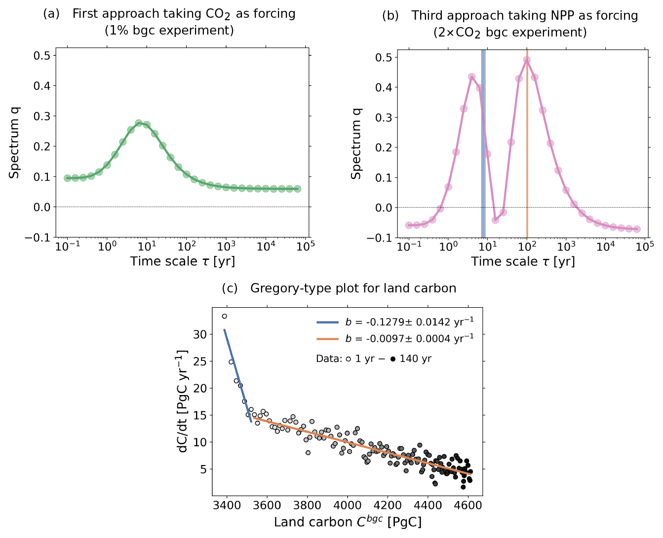
Figure 9Spectra associated with χNPP derived with different resolutions and a Gregory-type plot to identify the timescale structure of land carbon. (a) Spectrum derived with the first approach (taking CO2 as forcing) from the 1 % bgc experiment; (b) spectrum derived with the third approach (taking NPP as forcing) from the 2×CO2 bgc experiment; (c) Gregory-type plot of global land carbon against land–atmosphere carbon flux. Dots are the data, with the color scale from white to black indicating the evolution from 1 to 140 years. Values of b indicate the rate at which the time derivative of land carbon changes with respect to the land carbon itself. Ranges of timescales corresponding to each rate accounting for 1 standard deviation are shown in (b).
5.3 Checking the robustness of the spectrum via regional response functions
The robustness of this detailed spectrum can be further checked by a different method. In the following, we test this robustness by checking the consistency between the timescales of global and regional carbon responses.
To study regional carbon responses, we considered two regions: tropics and extra-tropics. Tropics were defined as the region between latitudes 30∘ S and 30∘ N, and extra-tropics as the remaining part of the globe. We then determined separately the linear response functions that characterize the land carbon response to NPP in the tropics and extra-tropics, defined, respectively, by
The data were taken once more from the 2×CO2 bgc experiment.
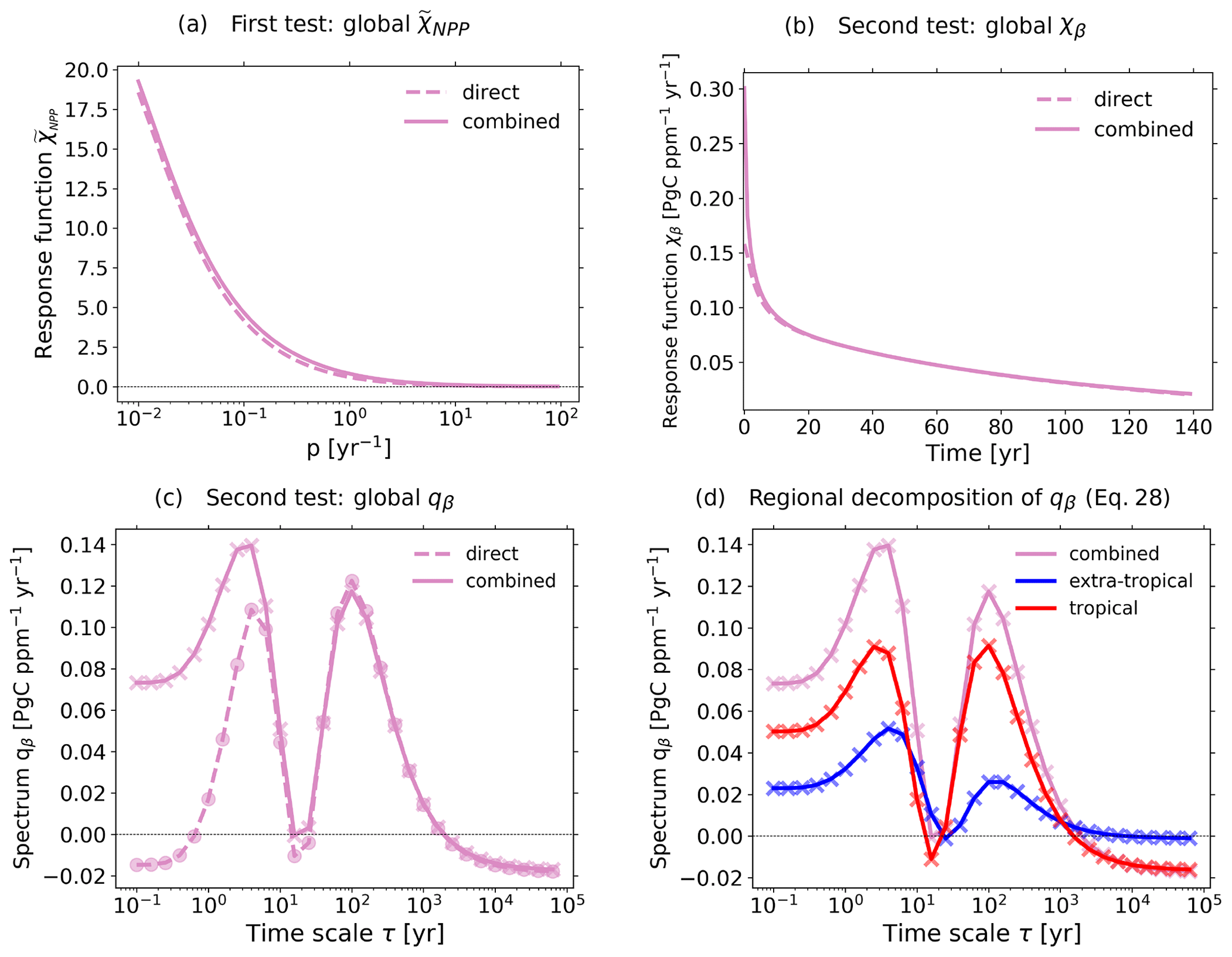
Figure 10Investigation of the land carbon response in the tropics and extra-tropics and how the regional response functions combine to the global response functions. The analysis is based on the 2×CO2 bgc experiment. (a) Laplace transform of global χNPP(t) obtained directly from the global carbon response and from combining the tropical and extra-tropical response functions; (b) χβ(t) obtained directly from the global carbon response and from combining the tropical and extra-tropical response functions; (c) as (b) but for qβ(τ); (d) decomposition of qβ(τ) into tropical and extra-tropical spectra (Eq. 31). In (c, d) the dots and crosses indicate the computed values, while the connecting lines are only inserted to guide the eye. For more details, see text.
Before assessing the robustness of the spectrum, we check the consistency between the regional and global response functions. In this test, we show that the global response function χNPP can be reconstructed by combining and . For this purpose, we write the global land carbon as the sum of the land carbon in the tropics and extra-tropics:
Plugging Eqs. (17), (22) and (23) in Eq. (24) and recognizing that gives
Applying a Laplace transform to both sides of Eq. (25) and reorganizing the resulting equation gives
Therefore, the Laplace transformed can be obtained from combining the NPP forcings and the response functions for the tropics and extra-tropics. Hence, if the response functions are correctly recovered by the RFI algorithm, Eq. (26) should hold at least approximately. In order to check this, we computed the Laplace transforms analytically by approximating the NPP forcings by step functions (since we take the 2×CO2 bgc experiment), and using Eq. (5) for the response functions. Figure 10a shows the quality of the result. The small discrepancy between obtained from the global carbon response and from combining the regional responses can be at least partially explained by the approximation error made to represent the forcings by a step function.
We now check the robustness of the land carbon spectrum by combining and to obtain χβ(t) and thereby qβ(τ). To this end, we first obtain the tropical and extra-tropical by applying Eq. (21):
Note that because CO2 is well mixed, , so that, by characterizing the tropical and the extra-tropical response to CO2, and are describing the response to a regionally correct perturbation. Using the response functions obtained from Eqs. (27) and (28), one can now write Eq. (14) for global, tropical and extra-tropical carbon. Plugging the result into Eq. (24) gives
Hence, one can infer that
Therefore, the global response function χβ(t) can be obtained from and . However, in addition, since χ(t) is given by Eq. (5), Eq. (30) implies that one can also obtain the global spectrum qβ(τ) by combining the regional spectra:
Therefore, using the recovered response functions for tropical and extra-tropical carbon one can obtain the global response function χβ and its associated spectrum qβ. Accordingly, in this test we check Eqs. (30) and (31). For the calculation of the derivatives in Eqs. (27) and (28) we fitted NPPtr=NPPtr(Catm) and NPPet=NPPet(Catm) once again by a polynomial of order 6 (which obtained the best results for global NPP in Fig. 7b) and took the derivatives from the fits. For χβ(t) we used the recovery with best quality from Fig. 7 (“NPP”). The spectra qβ(τ), and are obtained by scaling the spectra from χNPP(t), and by the respective derivatives , and Results are shown for χβ in Fig. 10b and for qβ in Fig. 10c. As seen in Fig. 10b, the reconstruction matches almost perfectly the values of χβ for times beyond about 20 years. Likewise, the spectrum qβ is almost perfectly reconstructed for timescales above 6 years, with a slight discrepancy between 15 and 25 years (see Fig. 10c). A larger disagreement is seen below 20 years for χβ and below 6 years for qβ. One of the reasons is that only little information is available for timescales smaller than 1 year because this is the time step taken for the data. However, Appendix D shows that timescales much shorter than the time step affect only χ(0). The main reason for the disagreement is that high frequencies (and thus small timescales) are the most problematic to recover due to the ill-posedness of the problem that obscures the signal particularly at high frequencies.
Despite the disagreement at small timescales, Fig. 10b and c add confidence that (1) the response functions for global, tropical and extra-tropical carbon can be trusted over mid to long timescales (Fig. 10b) and that (2) the two-peak spectrum obtained for global land carbon indeed characterizes the response, since its computation from two independent approaches (combining regional spectra in Fig. 10c and the Gregory-type plot in Fig. 9c) yield similar results with characteristic timescales matching the peaks of the spectrum.
5.4 Investigating the two-peak structure of the spectrum
The reasons for the two-peak structure of the land carbon spectrum are conceivable. In principle, one possibility could be that the short timescales reflect the carbon dynamics in the tropics, a region with higher temperatures and thus larger heterotrophic respiration rates (see, e.g., Raich and Potter, 1995), while the long timescales may originate from the carbon dynamics in the extra-tropics, where respiration rates are smaller due to lower temperatures. This hypothesis may be checked by examining Fig. 10d, which shows the contribution from the tropics and the extra-tropics to the land carbon spectrum (Eq. 31). However, as seen, the two peaks arise both in the tropical and in the extra-tropical spectrum, so that one cannot attribute each peak to a particular region. Therefore, this cannot be the explanation.
An alternative hypothesis is that the different peak timescales originate from the very different characteristic timescales of functionally different elements in the land carbon cycle such as leaves, wood, litter and soil. In the following we investigate whether this hypothesis can explain the two-peak structure.
For this purpose, we split the land carbon pools of the MPI-ESM into two groups (see Fig. 11). In the first group are the pools whose dynamics is governed by fast processes such as shedding and decomposition of leaves, thus the pools that respond at short timescales. These are the pools representing non-woody tissues in living vegetation (leaves, fine roots, sugars, and starches) and the associated litter. In the second group are the pools with dynamics determined by slow processes such as the decomposition of woody plant parts, hence the pools that respond at long timescales. These are the pools representing the wood in stems and coarse roots, the associated litter pools, and the soil carbon (humus).
Now, we separate the land carbon spectrum into contributions arising from each of these two groups. The land carbon response can be described as the sum of the collective responses from the pools with fast and those with slow dynamics:
In the linear response framework, the response of each term to NPP is given by
which implies
Finally, assuming that each response function in Eq. (34) is described by Eq. (5), we obtain the separation of the land carbon spectrum in terms of the contribution from each pool group:
Hence, if our hypothesis is correct, then the peak at short timescales should be explained by and the peak at long timescales should be explained by .
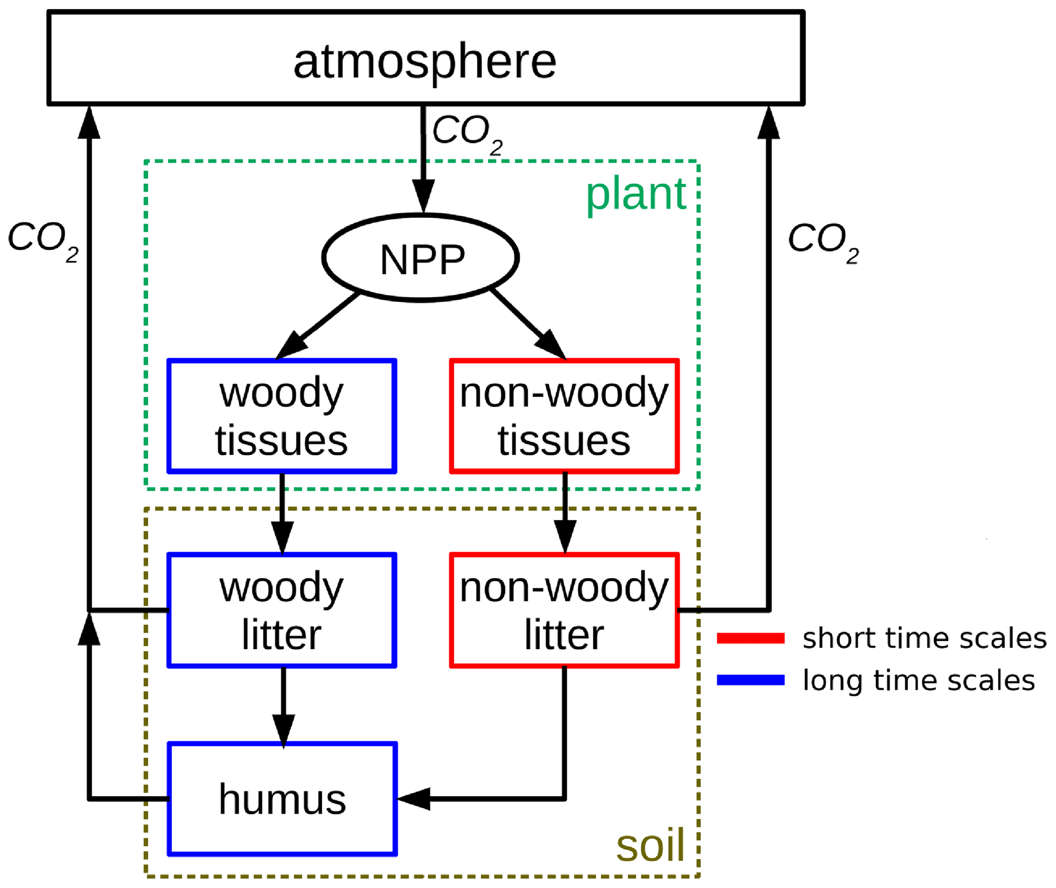
Figure 11Simplified pool scheme of the land carbon cycle in the MPI-ESM (see Appendix A) with pools split into two groups according to the characteristic timescales underlying their dynamics.
To proceed with the analysis we now need to obtain the spectra and . When investigating the tropical and extra-tropical land carbon, we obtained each regional spectrum individually by applying the RFI algorithm to the data from the tropical and extra-tropical responses. In principle one could proceed in the same way to separate contributions from the two pool groups, but, as will become clear below, this approach introduces slight inconsistencies between the separate recoveries that makes a quantitative comparison of the two contributions less reliable than the alternative method that we use in the following to separate the fast and slow components of qNPP.
The idea of this alternative approach is the following. Numerically the land carbon spectrum is given by the regularized solution (Eq. 6), i.e.,
where the regularization parameter λ is determined by the RFI algorithm. The land carbon response ΔCbgc is given by the sum (32) of the responses from the pools with fast and those with slow dynamics. Entering Eq. (32) into Eq. (36) yields
Therefore, by deriving the spectra and using the same regularization parameter λ employed for the land carbon spectrum qNPP,λ, we can in principle accurately reconstruct qNPP,λ from and .
By obtaining and in this way and combining them via Eq. (35) we show that qNPP,λ can indeed be very accurately reconstructed (Fig. 12a). This approach also leads to an almost perfect reconstruction of the response function χNPP via Eq. (34), as shown in Fig. 12b. Compared to our previous approach employed to reconstruct the global spectrum from the regional spectra (Eq. 31), this alternative approach gives a more accurate reconstruction because it takes the same regularization parameter λ for all qNPP,λ, , and , in contrast to the previous approach where λ was separately calculated by the RFI algorithm for each spectrum in Eq. (31).
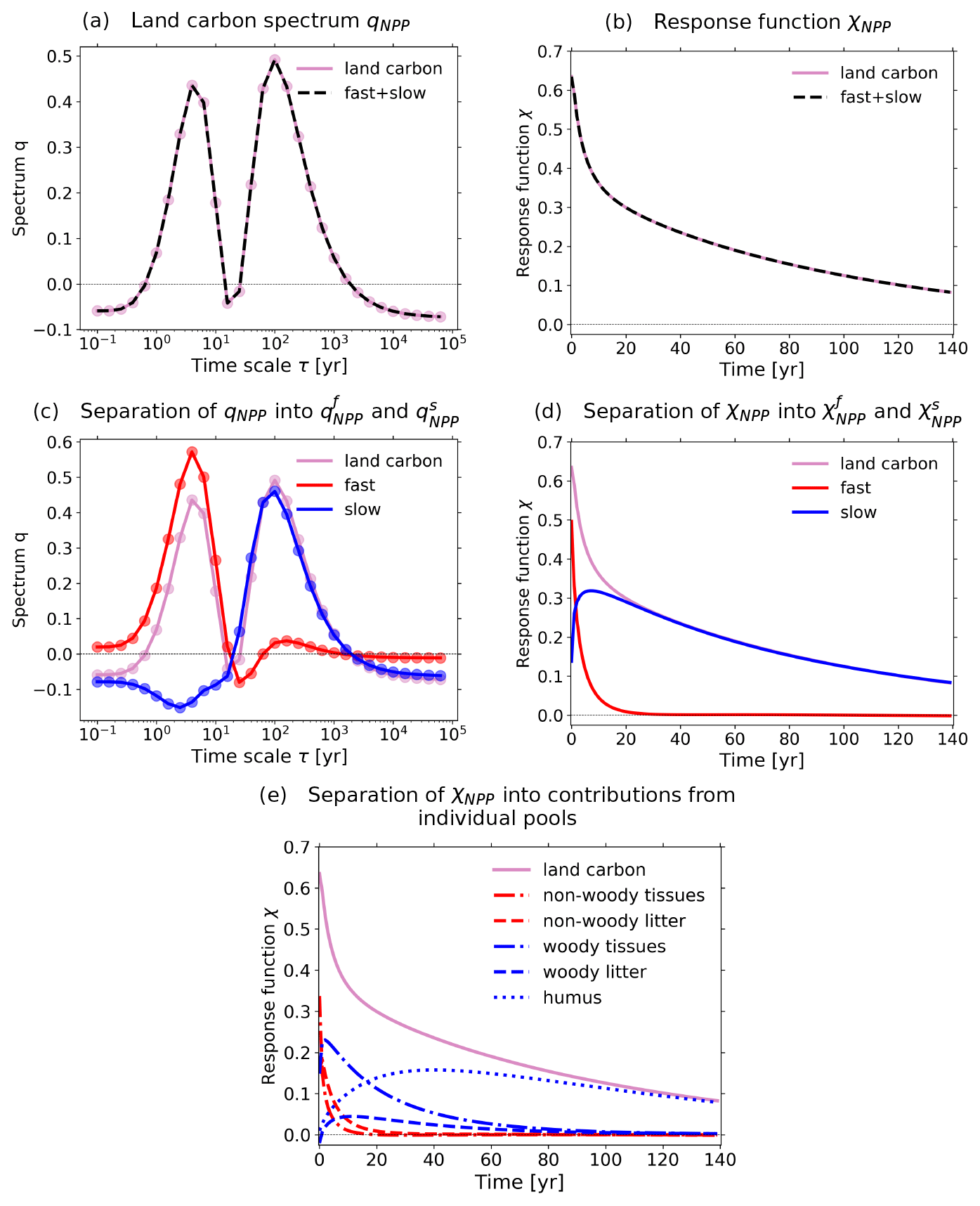
Figure 12Investigation of the contribution from the pools with fast dynamics (non-woody pools) and those with slow dynamics (woody and humus pools) to the land carbon spectrum. The analysis is based on the 2×CO2 bgc experiment. (a) Land carbon spectrum qNPP and its reconstruction via Eq. (35) from the fast and slow components; (b) response function χNPP and its reconstruction via Eq. (34) from the response functions for the fast and slow components; (c) separation of spectrum qNPP into and ; (d) separation of response function χNPP into and ; (e) separation of χNPP into contributions from the individual pools. For more details, see the text.
Now, the question is whether the spectra and can indeed explain each peak in the land carbon spectrum qNPP. To check this, in Fig. 12c we plot the three spectra. As seen, clearly the peak at short timescales of the land carbon spectrum arises mostly from the large peak in the fast-dynamics spectrum, while the peak at long timescales follows closely the large peak in the slow-dynamics spectrum. This result thus indicates that our hypothesis is correct, so that the two-peak spectrum indeed originates from the different characteristic timescales of functionally different elements in the land carbon cycle.
More insight into the dynamics of the land carbon can be gained by analyzing the different contributions to the response function χNPP shown in Fig. 12d and e. Figure 12d shows the contribution of the pools with fast dynamics and that of the pools with slow dynamics . We see that only dominates the response at times smaller than about 2 years. Further, for times larger than 25 years only contributes to the response. In Fig. 12e we further separate the response functions into the contributions from the individual pools, i.e.,
where is the response function for the non-woody tissues in living vegetation, for non-woody litter, for woody tissues in living vegetation, for woody litter, and for the humus pool. This more detailed separation shows that for long times the humus pool starts to dominate the response, so that at times larger than 100 years it gives the only contribution.
Although the γ and β values introduced by Friedlingstein et al. (2003) provide a useful framework for model intercomparison, they only characterize the sensitivity of a model for a particular perturbation scenario. Instead, one would like to characterize the sensitivity as an independent property of the carbon cycle. The dependence of γ and β on the considered scenario arises because of the internal memory of the system, i.e., because of the dependence of the response on past values of the perturbation. When the memory is taken into account, linear response functions arise as natural generalization of the γ and β sensitivities. However, a fundamental step for applying this generalized framework is to identify the appropriate linear response functions. In Part 1, we developed a method to identify linear response functions from data using only information from an arbitrary perturbation experiment and a control simulation. In that study, the robustness of the method in the presence of noise and nonlinearity was demonstrated in applications to data from perturbation experiments performed with a toy model.
6.1 Generalized land carbon sensitivities in the MPI-ESM
In the present study, we demonstrated that our RFI method can also be employed to derive response functions from C4MIP data. Here, we identified for the MPI-ESM, using data from standard 1 % experiments, the land carbon generalized sensitivities χγ and χβ, i.e., the linear response functions that generalize the γ and β sensitivities for land carbon. The robustness of the identified generalized sensitivities was demonstrated by their ability to predict the response from experiments not used for the identification (Sects. 3 and 4). With the aid of additional experiments, we estimated the linear regime that gives the range of forcing strengths for which each generalized sensitivity can predict model responses. For χγ, results indicate a linear response at least until the end of the 1 % experiment, corresponding to temperature perturbations of around 6 K. For χβ, the estimate is for CO2 perturbation strengths up to 100 ppm. In addition, we analyzed different approaches that may be employed to improve the quality of the recovery of the response functions. For χγ, taking the response from a 2×CO2 experiment demonstrated to give smaller prediction errors for every response evaluated, suggesting that this type of experiment also gives a better recovery. For χβ, the estimated linear regime of only 100 ppm indicates that for larger forcing strengths nonlinearities are present in the response that deteriorate the recovery of χβ. To circumvent such nonlinearities and thus improve the recovery, we identified χβ by using NPP instead of CO2 as forcing. We found that by this approach an approximately linear response is found over the whole 1 % experiment, i.e., until CO2 perturbations of about 850 ppm. This result suggests that nonlinearities in the biogeochemical response of land carbon can to a large extent be explained by the nonlinear relationship between NPP and CO2. This approach of using NPP as forcing instead of CO2 yielded the best recovery for χβ. Evidences for this conclusion are the quality of its prediction and the detailed spectrum it yields for the response.
6.2 Spectrum of land carbon timescales
Obtaining the spectrum of the response is an additional advantage of the RFI method. Most methods in the literature either recover χ(t) pointwise – and therefore do not give the spectrum – or try to fit it with few exponents without accounting for ill-posedness, which does not give reliable results for the spectrum (see, e.g., the famous example from Lanczos, 1956, p. 272). In the application to the MPI-ESM, obtaining the spectrum has proven advantageous for two reasons. First, it allows one to formally extend the recovery of the response function beyond the time range of the length of the underlying time series. Results from such an extension (Fig. 8a and b) demonstrated that the recovered response function contains information on times reasonably longer than the time series length used for the recovery.
Second, the spectrum gives valuable insight into the internal dynamics of the system. In particular, for our application the spectrum gives the most relevant timescales for the land carbon response on a global or regional level. The spectrum associated with the best recovery of χβ showed two peak timescales for the global response: one around 4 and another around 100 years (Sect. 5).
To obtain evidence for the robustness of this result, we showed that it is possible to reconstruct the global spectrum from the recovered tropical and extra-tropical spectra (see Fig. 10c), and that similar timescale ranges can be obtained via a Gregory-type approach (see Fig. 9b and c). Further, we demonstrated that the recovered tropical and extra-tropical response functions combine to the identified global response functions, indicating consistency between regional and global recovery (see Fig. 10a and b).
We then proceeded to investigate the reason for the two-peak structure of the spectrum. To this end, we separated the land carbon response into the response from pools with fast dynamics (non-woody vegetation tissues and associated litter) and the response from pools with slow dynamics (woody vegetation tissues, woody litter, and humus). By analyzing the spectrum for each of these responses we showed that the peak at short timescales of the land carbon spectrum arises mostly from the contribution of the pools with fast dynamics, while the peak at long timescales follows closely the contribution from the pools with slow dynamics. This investigation therefore suggests that the two-peak spectrum results from the different contributions of functionally different elements of the land carbon cycle. Analysis of the response functions showed that the pools with fast dynamics dominate the land carbon response only for times below 2 years. Further, for times larger than 25 years only the pools with slow dynamics contribute to the response, and from 100 years onwards the contribution comes solely from the humus pool.
We remark that results for the spectrum should be always interpreted with care, since deriving the spectrum may be a more complicated problem than deriving the response function. This is partially explained by the degree of ill-posedness of each problem. In deriving the response function from Eq. (3), one is solving a deconvolution problem, which is known to be ill-posed because of the smoothing property of the convolution operator (e.g., Landl et al., 1991; Bertero et al., 1995; Hansen, 2002). On the other hand, by deriving the spectrum from Eqs. (3) and (5), one is solving not only a deconvolution (Eq. 3), but also a type of inverse Laplace transform (to obtain the spectrum from the response function 5), which is known to be extremely ill-posed because of the smoothing property of the Laplace operator (e.g., McWhirter and Pike, 1978; Istratov and Vyvenko, 1999). As a result, deriving q(τ) from the data ΔY(t) involves two smoothing operations, namely the Laplace transform and convolution, whereas deriving χ(t) from ΔY(t) involves only convolution, so that the problem of finding q(τ) may be more ill-posed than that of finding χ(t). This difficulty was exemplified by results from Appendices D and E, which discuss cases where the response function can be perfectly recovered but the recovered spectrum is relatively poor.
Another worthwhile comment is that, in comparison to the widely used assumption that the spectrum can be described by only a few exponents (Maier-Reimer and Hasselmann, 1987; Enting and Mansbridge, 1987; Enting, 1990; Joos et al., 1996, 2013; Pongratz et al., 2011; Colbourn et al., 2015; Lord et al., 2016), our assumption of a continuous spectrum (ansatz 5) has some advantages. First, by our approach one circumvents the complication of determining the number of exponents. This leads to a linear problem and thereby to a more transparent method (see Part 1, Sect. 3.1). Second, our ansatz better describes the expectation that variables integrated over many different climate zones are composed by a large range of timescales. If, in contrast to these expectations, the underlying spectrum has only few timescales, results in Appendix E show that our approach may still yield a reasonable recovery.
6.3 Outlook
In this study we investigated the generalized γ and β sensitivities that solve the scenario dependence problem noted, e.g., by Gregory et al. (2009) and Arora et al. (2013) to linear order in the perturbation – an approach that can in principle be extended to higher orders (Ruelle, 1998; Lucarini, 2009). By demonstrating how to successfully recover generalized sensitivities, this study paves the way for their future application in studying the dynamics of the combined carbon climate system in different Earth system models. Applying our RFI method, we showed for the MPI-ESM that one can obtain these sensitivities from standard C4MIP 1 % simulations. In addition, the estimates for the linear regime obtained by employing the recovered sensitivities to predict additional experiments give a hint at the range of perturbation strengths for which this generalized framework might be valid for other models as well for which data from additional experiments necessary to determine this linear regime are not available. Since the process descriptions of the land carbon cycle are quite similar in different models, it may be assumed that the linear range estimates obtained for MPI-ESM in the present study also apply to other models. Considering the radiative land carbon response, for other models their χγ should thereby also fully characterize the response to temperature up to at least 6 K. As a consequence, in models with temperature responses similar to or weaker than the MPI-ESM, χγ can as for the MPI-ESM be recovered taking the full time series from the 1 % experiment. Analogously, considering the generalized sensitivity χβ, the experience presented in the present study for the MPI-ESM suggests that also for other models the response to CO2 perturbations is linear up to 100 ppm. As a consequence, χβ can be recovered taking data from the 1 % experiment for the first 30 years. Alternatively, as discussed in Sect. 4, the time range for the recovery of χβ can be extended if one takes as forcing NPP instead of CO2 (third approach investigated in Sect. 4). For models with NPP responses similar to or weaker than the MPI-ESM, by this approach χβ can be recovered taking the full time series from the 1 % experiment. Still, as the relatively successful predictions in Fig. 8b suggest, even if χβ is recovered by taking CO2 as forcing for only 30 years of the 1 % experiment (first approach investigated in Sect. 4), it may still contain sufficient information to predict responses of the model for a time range of 140 years.
In the present investigation we have studied rather idealized simulations where only perturbations in atmospheric CO2 are acting on the climate system. A possible next step towards the application of our sensitivity analysis to more realistic scenarios could be to consider historical experiments where other perturbations such as land-use change and non-CO2 greenhouse gases are also applied. To this end, a combination of different response functions should be considered to take separately into account the response of the system to each perturbation (as, e.g., in Bódai et al., 2020). Another possible extension of our study could be to employ response functions to study the spatial dynamics of the carbon cycle. We have shown a simple example of this type of application by looking at the responses for tropics and extra-tropics, but in the literature one also finds applications to study the response latitudinally resolved and even globally at grid-cell level (Thompson and Randerson, 1999; Lucarini et al., 2017).
However, in addition to the carbon cycle sensitivities considered here, our RFI method may be applied to investigate different aspects of climate and the carbon cycle. Ragone et al. (2016) have shown how the linear response framework generalizes the concept of equilibrium climate sensitivity (ECS) and transient climate response (TCR). Originally, ECS is defined as the response of global temperature to an instantaneous doubling of atmospheric CO2 from its pre-industrial value, while TCR is the temperature response to a doubling of CO2 after a 1 % per year increase. Within the generalized framework, the ECS and TCR are shown to be only particular values encoded in a linear response function.
Linear response functions can also be useful in studying “committed changes” (Wigley, 2005; Plattner et al., 2008; Jones et al., 2009; Mauritsen and Pincus, 2017). As shown by Ragone et al. (2016), the concept of climate inertia (closely related to committed changes) can be explicitly described within the linear response framework. Since the linear response function describes the delayed response of the system to a perturbation, by deriving this function one also has at hand the information of how the system reacts once the perturbation – for instance CO2 emissions – ceases.
Further, linear response functions can help understanding the concept of “emergent constraints” (Nijsse and Dijkstra, 2018). Recent studies have shown how to obtain from response functions derived from conceptual models emergent constraints for the real Earth system (Cox et al., 2018; Williamson et al., 2019). With the method developed here, in principle such types of analyses may be carried out employing instead response functions derived from Earth system models.
As a result of accounting for the memory of the system, the linear response function gives information on the strength of the response at all internal timescales covered by the time series underlying its recovery and probably even slightly longer (see Fig. 8b). Using our method, in principle one can even compare the spectra of timescales from models to those from observations (e.g., Forney and Rothman, 2012b). The method presented here may also be applied to analyze changes in age and transit time distributions of carbon in different models, since these distributions can be derived directly from linear response functions (Thompson and Randerson, 1999).
In all of the mentioned examples, the generality of the RFI method allows for the derivation of the appropriate linear response functions for any model by taking only data from an arbitrary perturbation experiment and a control experiment. Such generality opens the possibility of combining the linear response framework, which has been gaining increasing attention due its wide applicability in climate science (e.g., Lucarini, 2009; Lucarini and Sarno, 2011; Lucarini et al., 2014, 2017; Ragone et al., 2016; Aengenheyster et al., 2018; Ghil and Lucarini, 2020; Lembo et al., 2020; Bódai et al., 2020), with model intercomparison studies, hopefully leading to a deeper understanding of critical differences encountered across models.
In this Appendix we give a brief description of the model employed in this study: the Max Planck Institute for Meteorology Earth System Model (MPI-ESM; for more details see Giorgetta et al., 2013). The MPI-ESM consists of the coupled general circulation models ECHAM6 (Stevens et al., 2013) for atmosphere, at T63/1.9∘ horizontal resolution with 47 vertical levels, and MPIOM (Jungclaus et al., 2013) for ocean, with a nominal resolution of 1.5∘ with 40 vertical levels. In addition, the MPI-ESM includes the subsystems JSBACH (Reick et al., 2013; Schneck et al., 2013), a land and vegetation model, and the marine biogeochemistry model HAMOCC (Ilyina et al., 2013). JSBACH and HAMOCC describe, respectively, the land and ocean carbon cycle in the MPI-ESM. Thus, of particular interest for our study is the subsystem JSBACH. JSBACH simulates fluxes of energy, water, momentum and CO2 between the land surface and atmosphere. To represent subgrid scale heterogeneity, each grid cell of the land surface is divided into tiles, each tile being associated with a vegetation type (or “plant functional type”). The photosynthesis scheme follows Farquhar et al. (1980) and Collatz et al. (1992). The land carbon structure is divided into three vegetation pools (living tissues, carbohydrate and starch storage, and wood), four aboveground and belowground pools for litter from woody and non-woody parts and a pool for soil carbon (humus). In addition, JSBACH includes a dynamic vegetation scheme that allows for simulating changes in vegetation cover driven by climate.
In this Appendix we show that linear response functions indeed generalize Friedlingstein α–β–γ sensitivities. We explain this by taking the β sensitivity of land carbon uptake as an example. The calculation of β is based on an experiment where the CO2 rise acts only biogeochemically, i.e., concerning the land carbon via the photosynthesis of plants. Calling ΔCbgc(t) the difference in land carbon between the perturbed and the control simulation, β is defined as
where t is the time in years elapsed since the perturbation was switched on, and ΔCatm(t) is the change in CO2 concentration when increasing atmospheric CO2 each year by 1 % starting from its pre-industrial value of the control simulation. In the framework of linear response, one can understand ΔCatm(t) as perturbation and ΔCbgc(t) as response, so that the response formula reads
This equation defines χβ(t) as the linear response function describing the biogeochemical response of land carbon to any type of CO2 perturbation ΔCatm(t), as long as the perturbation is sufficiently weak. Employing in particular the percent perturbation from Eq. (B1), β(t) is thus obtained from the linear response function χβ(t) as
In this way, χβ(t) can be understood as a generalization of β(t) that gives not only the response to percent-type perturbations, but also to other perturbations. Accordingly, χβ(t) characterizes system properties independent of the type of perturbation, in contrast to β(t).
In this Appendix it is shown that the response function χβ(t) is monotonic, as claimed in Sect. 2.1. The argument here is actually more general, namely that the response function to changes in the input of the system (for land carbon, the net primary production) is monotonic. Since χβ(t) is related to χNPP(t) by Eq. (21), the monotonicity property transfers to χβ(t).
Let the linear response of land carbon be described by Eq. (17):
where for simplicity we assume that η(t) is small, so that it can be neglected. If NPP is a Dirac delta function ΔNPP(t)=δ(t), then the response is given by ΔCbgc(t)=χNPP(t). Therefore we can interpret the response function χNPP(t) as follows: if a certain number of carbon atoms enter the biosphere at time t=0, the response function χNPP(t) gives the fraction of these atoms still left in the biosphere at time t.
Let p(t)dt be the probability that an atom that entered the system at time t=0 will leave it at time t. Then
is the probability that an atom that entered the system at time t=0 will leave the system until time t. Hence from the interpretation of χNPP(t) above,
From Eqs. (C2) and (C3) it follows that
However, since the probability density function , then , i.e., χNPP(t) decays monotonically towards zero. Therefore, because χβ(t) is simply a scaling of χNPP(t) given by Eq. (21), χβ(t) also decays monotonically towards zero.
Timescales much longer or much shorter than the timescales covered by data cannot be correctly recovered in the spectrum. Nevertheless, in this Appendix we show that the wrong recovery of these extreme timescales does not strongly affect the recovery of χ(t). These considerations add to the footnote remark in Sect. 5 where we claim that such extreme timescales can be safely ignored.
First, we consider the case where the response has timescales much longer than those covered by data. Let χ at time T be given by
Let T be the time series length and assume that q(τ) has significant contributions at timescales τ≥τL with τL≫T. Then (D1) can be written as
where was used in the second integral because τL≫T. Thereby the second term in the right-hand side of (D2) is just a constant offset
Hence, for internal timescales much longer than the time series length T, the correct recovery of the individual q(τ) values is not relevant for the derivation of χ(t), as long as those values combine to the correct offset in Eq. (D3). Note that because this argument is based on the condition τL≫T, it applies not only to χ(T), but also to all χ(t), t<T.
Now, we consider the case where the response has timescales much smaller than those covered by data. Let , where Δt is the time step and i∈IN. If q(τ) has significant contributions at timescales τ≤τS with τS≪Δt, then for i>0 Eq. (5) can be written as
where was used for τ<τS because τS≪Δt. As a result, values of q(τ) are irrelevant to χ(t) for almost every i. The only exception is i=0, where one has
Hence, for timescales much shorter than the time step Δt, the correct recovery of the individual q(τ) values is not relevant for the derivation of χ(t) as long as those values combine with the other recovered values of q(τ) to the correct χ(0) in Eq. (D5). As shown by Eq. (D4), if they combine to the wrong value, only the recovery of χ(0) is affected.
Therefore, in principle χ(t) can also be correctly recovered when the response contains much longer and much shorter timescales than those covered by data, as long as the recovered q(τ) values at these extreme timescales combine to the correct values of the offset in Eq. (D3) and χ(0) in Eq. (D5). In Fig. D1 we show an example of recovery of the spectrum and response function in such a case. For the recovery we took data with from the 1 % experiment with our toy model (see Part 1). As seen, the spectrum can only be partially recovered (Fig. D1a). The recovery wrongly estimates spectral contributions at timescales longer and shorter than those covered by data, i.e., timescales larger than the time series length T=140 and smaller than the time step Δt=1. In addition, the existence of such spectral contributions at timescales not covered by data seems to also deteriorate the recovery of the spectrum at the timescales actually covered by data: in the region , despite the high SNR the recovered spectrum matches the true spectrum only partially. This is probably a compensation effect where wrong information shows up in the recovered spectrum to compensate missing information on the response function. For instance, to obtain the correct χ(0), only Eq. (D5) is needed but not the correct recovery of all timescales. The same goes for obtaining the correct offset: only Eq. (D3) is needed but not the correct recovery of all timescales from τL onwards.
Figure D1b shows the quality of the recovery of the response function χ(t). The recovered q(τ) values at long timescales, although individually wrong, combine to the correct offset in Eq. (D3): the “height” of the recovered response function matches almost perfectly that of the true response function (compare, e.g., the value at t=140 for the true and recovered response function). On the other hand, χ(0) is not perfectly recovered (compare the difference at t=0 between the true and recovered response functions), meaning that the sum in Eq. (D5) is incorrect. Nevertheless, the recovered value is still reasonably close to the true value. Except for this small error at χ(0), the overall recovery of the response function is almost perfect.
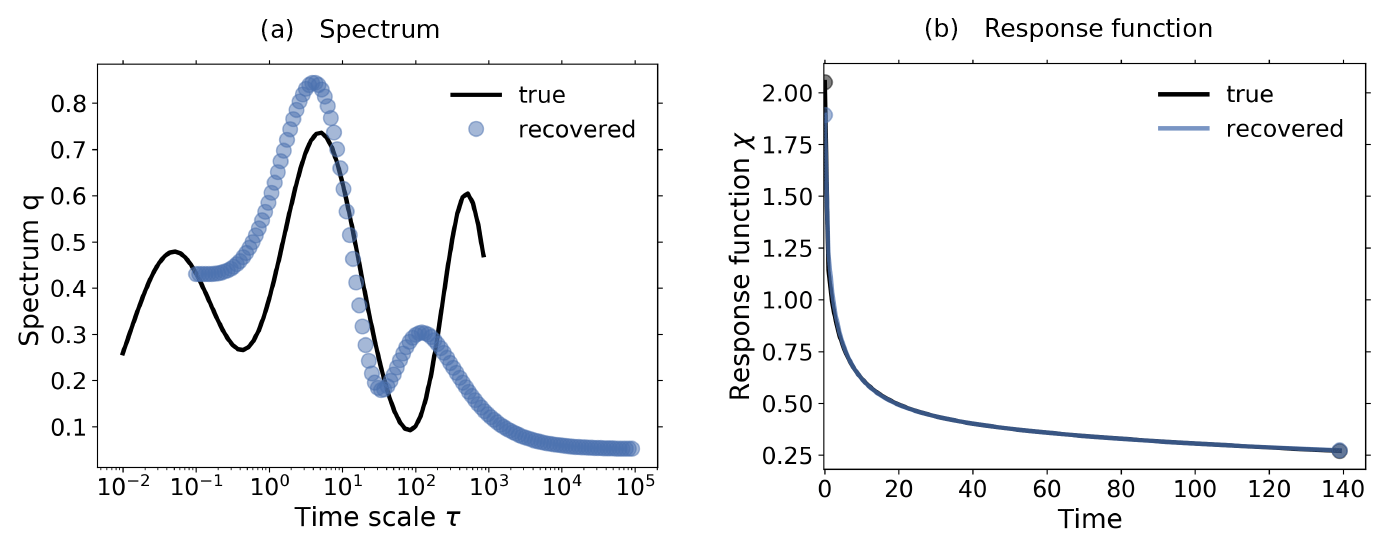
Figure D1Recovery of spectrum and χ(t) taking a true spectrum with contributions at timescales much longer and much shorter than the timescales covered by data. For the recovery, data with from the 1 % experiment with the toy model (see Part 1) was taken (time series length T=140 and time step Δt=1). RFI parameters are taken as in Part 1 except for M=140. The recovered spectrum matches only partially the true spectrum. Nevertheless, the response function χ(t) is almost perfectly recovered.
Therefore, as claimed in Sect. 5, this numerical example shows that even though very long and very short timescales cannot be correctly recovered in the spectrum, they do not strongly influence the recovery of χ(t). This is because they only influence the offset in Eq. (D3) and χ(0) in Eq. (D5), and those two values seem to be reasonably well recovered numerically.
This Appendix gives numerical evidence for the claim in Sect. 6 that although the RFI method assumes that the response has a continuous spectrum of many timescales, for sufficiently good signal-to-noise ratio the recovered continuous spectrum may also give a reasonable approximation to an underlying discrete spectrum of only few timescales.
Before we give numerical examples, one must first understand the limitations of the recovery of the spectrum. As explained in Part 1, the spectrum q(τ) can only be completely recovered (for sufficiently high SNR) if it is dominated by the first components of expansion (Eq. 6). By Hansen's observation (Hansen, 1989, 1990, see Part 1), this means that the spectrum must be dominated by low frequencies; i.e., it must be to some extent smooth. However, an underlying discrete spectrum implies a spectrum that is instead given by “spikes” in the timescale domain. Such “spikes” can only be described by high-frequency components of Eq. (6). Therefore, a discrete spectrum can be only partially recovered. To obtain a sufficiently good recovery, the solution (Eq. 6) must contain many components. Hence, the data must have a sufficiently high signal-to-noise ratio. The explanation for this conclusion is the following: if many components in Eq. (6) must be recovered, the regularization parameter must be small; but a small regularization parameter requires a small noise level (see Theorem 3.3.1 in Groetsch, 1984).
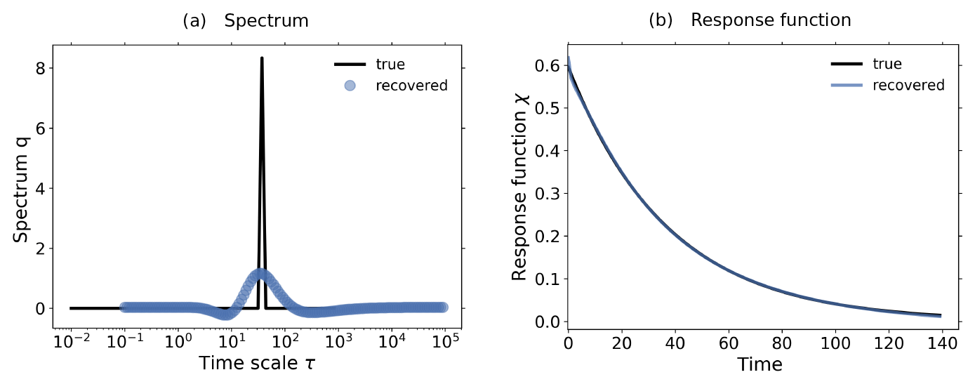
Figure E1Spectrum qλ and response function χ(t) recovered from a 1 % experiment performed with the toy model described in Part 1 taking an underlying discrete spectrum with one timescale τ=37. The data were taken with .

Figure E2Spectrum qλ and response function χ(t) recovered from a 1 % experiment performed with the toy model described in Part I taking an underlying discrete spectrum with two timescales τ=7 and τ=100. The data were taken with .
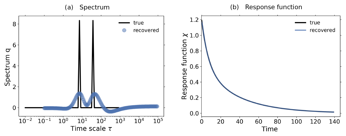
Figure E3Spectrum qλ and response function χ(t) recovered from a 1 % experiment performed with the toy model described in Part 1 taking an underlying discrete spectrum with two timescales τ=7 and τ=37. The data were taken with .

Figure E4Spectrum qλ and response function χ(t) recovered from a 1 % experiment performed with the toy model described in Part 1 taking an underlying discrete spectrum with two timescales τ=37 and τ=100. The data were taken with .
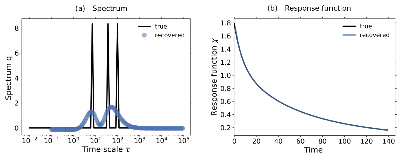
Figure E5Spectrum qλ and response function χ(t) recovered from a 1 % experiment performed with the toy model described in Part 1 taking an underlying discrete spectrum with three timescales τ=7, τ=37, and τ=100. The data were taken with .
With this in mind, we show in Figs. E1–E9 that at least smooth approximations to an underlying discrete spectrum can be obtained. For the results we took data with from different experiments performed with the toy model described in Part 1. Since the aim is to recover discrete spectra, a larger number of timescales M gives a better resolution. Therefore, we take M=140. All other RFI parameters are taken according to Part 1. Also, monotonicity needed not to be taken into account (step 6 of Fig. 1 in Part 1).
Figures E1–E6 show results for taking data from a 1 % experiment and Figs. E7–E9 from a 2×f0 experiment. We start with one timescale τ=37 (Fig. E1). As expected, the spike cannot be perfectly recovered, but the recovery gives a smooth approximation to it, with the peak coinciding approximately with the “true” value. On the other hand, the response function is almost perfectly recovered. This is a result of the ill-posedness of Eq. (5): in the same way that high frequencies of the spectrum are suppressed in the data by Eq. (3), they are also suppressed in the response function by Eq. (5) (see Groetsch, 1984, Sect. 1.1). Therefore, both the true spectrum and its smooth recovery result in practically the same response function.
In Fig. E2, the true spectrum has two timescales, this time at τ=7 and τ=100. Similarly to Fig. E1, the timescales are recovered by a smooth approximation with peaks approximately at the true values. Also similarly to Fig. E1, the response function is almost perfectly recovered. A similar result is obtained if we take timescales that are a bit closer together, as seen in Fig. E3 (τ=7 and τ=37). Nevertheless, now the peak for the longer timescale is a worse approximation, and there is a slightly pronounced negative peak that does not reflect the true spectrum.
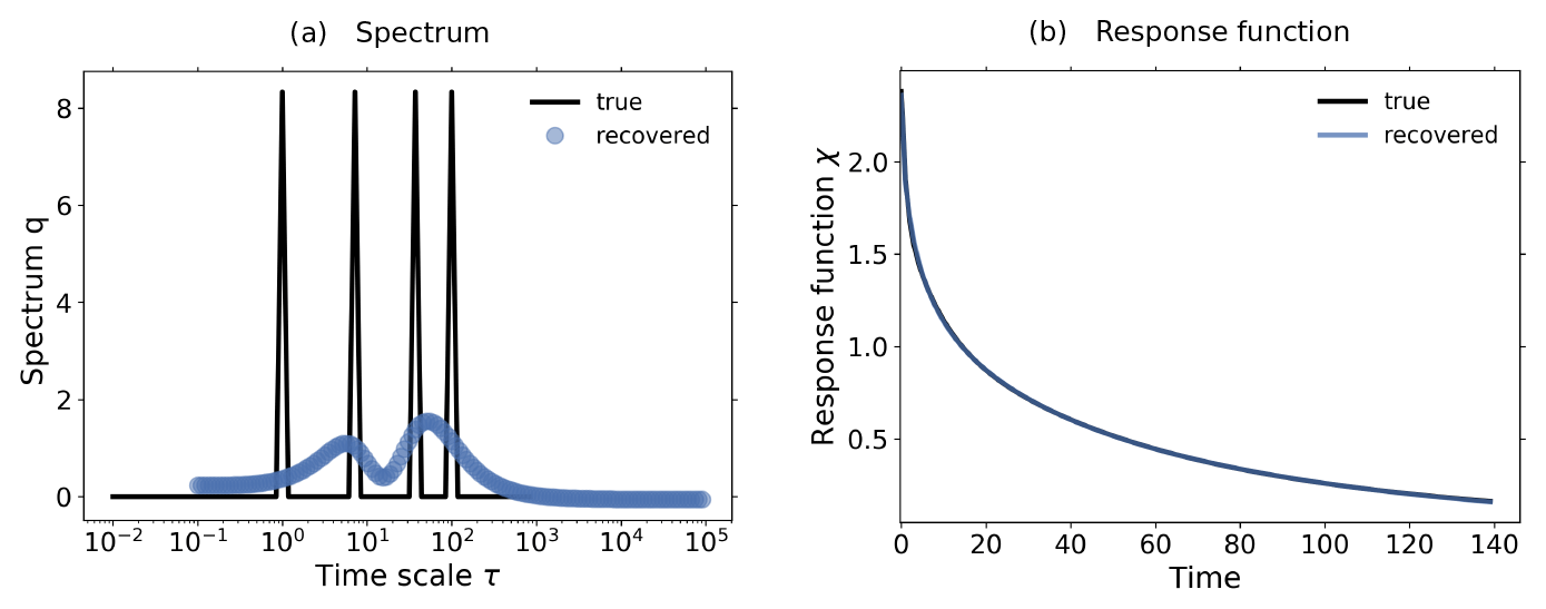
Figure E6Spectrum qλ and response function χ(t) recovered from a 1 % experiment performed with the toy model described in Part 1 taking an underlying discrete spectrum with four timescales τ=1, τ=7, τ=37, and τ=100. The data were taken with .
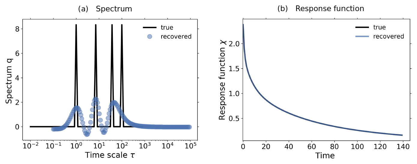
Figure E7Spectrum qλ and response function χ(t) recovered from a 2×f0 experiment performed with the toy model described in Part 1 taking an underlying discrete spectrum with four timescales τ=1, τ=7, τ=37, and τ=100. The data were taken with .
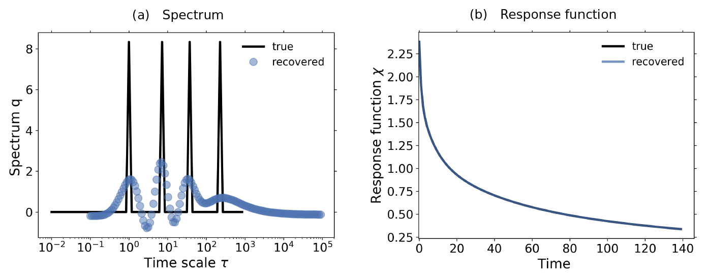
Figure E8Spectrum qλ and response function χ(t) recovered from a 2×f0 experiment performed with the toy model described in Part 1 taking an underlying discrete spectrum with four timescales τ=1, τ=7, τ=37, and τ=228. The data were taken with .
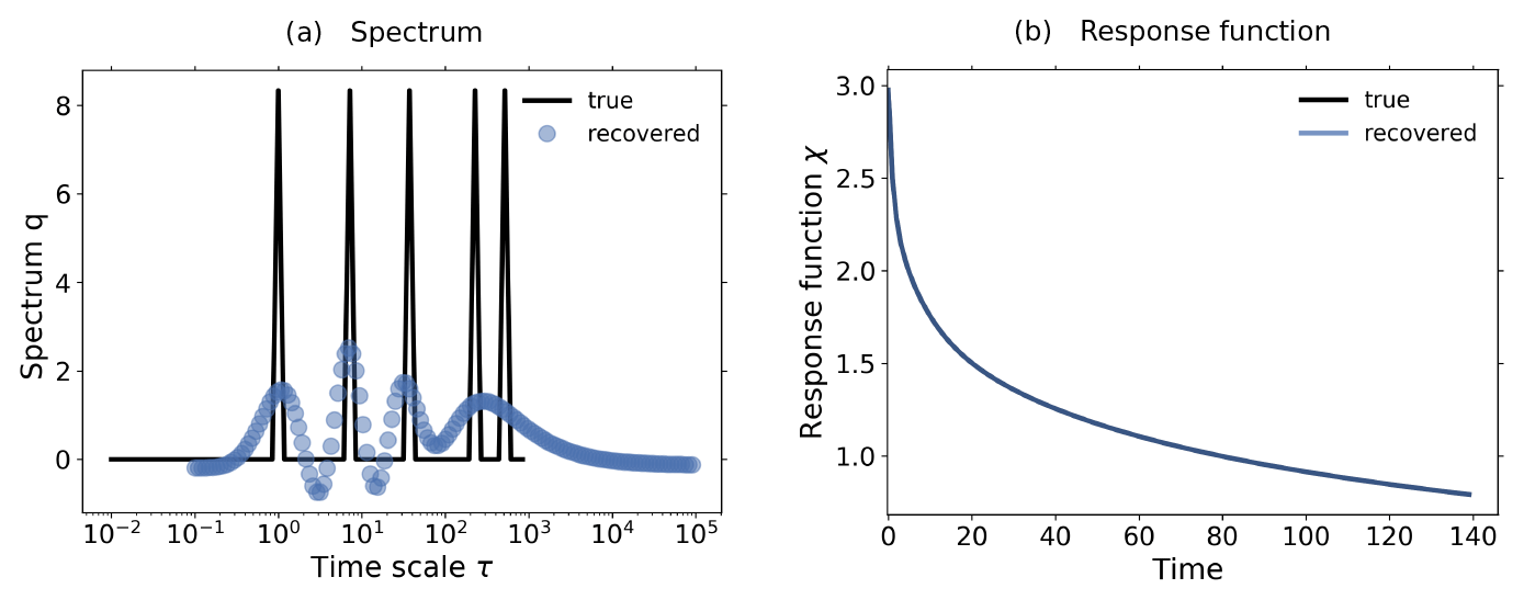
Figure E9Spectrum qλ and response function χ(t) recovered from a 2×f0 experiment performed with the toy model described in Part 1 taking an underlying discrete spectrum with five timescales τ=1, τ=7, τ=37, τ=228, and τ=518. The data were taken with .
In Fig. E4, we take instead timescales τ=37 and τ=100. Here, the resolution is not sufficiently high for a recovery of each timescale separately. Instead, the recovered spectrum shows only one mode that spans both spikes. Once more the response function can be almost perfectly recovered. Taking the three timescales τ=7, τ=37, and τ=100 (Fig. E5), the smooth recovery shows only two modes: one at τ=7 with peak almost coinciding with the true value, and another with peak in between τ=37 and τ=100. If one in addition considers a fourth timescale τ=1 (Fig. E6), once more the recovery shows only two modes. However, now the mode at shorter timescales displays a longer tail that spans both τ=7 and τ=1.
The situation changes when we take for the recovery the 2×CO2 experiment. According to the Laplace transform analysis in Sect. 3, data from this experiment should give more information on small timescales. Figure E7 shows that this is indeed the case: in contrast to the recovery from Fig. E6, now the timescale τ=1 is also recovered. On the other hand, now there are two small negative peaks that do not reflect information from the true spectrum. Also, the resolution is not sufficiently good to recover separately the two peaks at long timescales. However, if the longest timescale is increased from τ=100 to τ=228 (Fig. E8), a small peak can be seen around this timescale. In addition, now the peak at τ=37 matches slightly better the true value. In Fig. E9 we add another timescale, now at τ=518. We see that although this timescale cannot be recovered separately from τ=228, the peak at long timescales is more pronounced. This is in contrast with the fact that the time series used for the recovery reaches only t=140, indicating that the method can recover information on timescales even longer than the time series length. This is in agreement with the conclusions from Sect. 4, where in one case χβ(t) was recovered from a time series with only 30 years but could recover responses for t=140 years (see Fig. 8b).
The software code and information on how to obtain the data used in this study can be found at http://hdl.handle.net/21.11116/0000-0008-0F06-2 (last access: 6 October 2021; Torres Mendonca et al., 2021b).
The ideas for this study were jointly developed by all the authors. GTM conducted the study and wrote the first draft. All the authors contributed to the final manuscript.
The authors declare that they have no conflict of interest.
Publisher's note: Copernicus Publications remains neutral with regard to jurisdictional claims in published maps and institutional affiliations.
We would like to thank Andreas Chlond and also two anonymous referees for proposing revisions that considerably improved the quality of the manuscript.
The article processing charges for this open-access publication were covered by the Max Planck Society.
This paper was edited by Ilya Zaliapin and reviewed by two anonymous referees.
Adloff, M., Reick, C. H., and Claussen, M.: Earth system model simulations show different feedback strengths of the terrestrial carbon cycle under glacial and interglacial conditions, Earth Syst. Dynam., 9, 413–425, https://doi.org/10.5194/esd-9-413-2018, 2018. a, b
Aengenheyster, M., Feng, Q. Y., van der Ploeg, F., and Dijkstra, H. A.: The point of no return for climate action: effects of climate uncertainty and risk tolerance, Earth Syst. Dynam., 9, 1085–1095, https://doi.org/10.5194/esd-9-1085-2018, 2018. a
Alexandrov, G., Oikawa, T., and Yamagata, Y.: Climate dependence of the CO2 fertilization effect on terrestrial net primary production, Tellus B, 55, 669–675, 2003. a, b
Anav, A., Friedlingstein, P., Kidston, M., Bopp, L., Ciais, P., Cox, P., Jones, C., Jung, M., Myneni, R., and Zhu, Z.: Evaluating the land and ocean components of the global carbon cycle in the CMIP5 earth system models, J. Climate, 26, 6801–6843, 2013. a
Arora, V. K., Boer, G. J., Friedlingstein, P., Eby, M., Jones, C. D., Christian, J. R., Bonan, G., Bopp, L., Brovkin, V., Cadule, P., Hajima, T., Ilyina, T., Lindsay, K., Tjiputra, J. F., and Wu, T.: Carbon–concentration and carbon–climate feedbacks in CMIP5 Earth system models, J. Climate, 26, 5289–5314, 2013. a, b, c, d, e, f
Arora, V. K., Katavouta, A., Williams, R. G., Jones, C. D., Brovkin, V., Friedlingstein, P., Schwinger, J., Bopp, L., Boucher, O., Cadule, P., Chamberlain, M. A., Christian, J. R., Delire, C., Fisher, R. A., Hajima, T., Ilyina, T., Joetzjer, E., Kawamiya, M., Koven, C. D., Krasting, J. P., Law, R. M., Lawrence, D. M., Lenton, A., Lindsay, K., Pongratz, J., Raddatz, T., Séférian, R., Tachiiri, K., Tjiputra, J. F., Wiltshire, A., Wu, T., and Ziehn, T.: Carbon–concentration and carbon–climate feedbacks in CMIP6 models and their comparison to CMIP5 models, Biogeosciences, 17, 4173–4222, https://doi.org/10.5194/bg-17-4173-2020, 2020. a, b, c, d, e
Bertero, M.: Linear Inverse and Ill-Posed Problems, in: Advances in Electronics and Electron Physics, vol. 75, Academic Press, New York, NY, 1–120, https://doi.org/10.1016/S0065-2539(08)60946-4, 1989. a
Bertero, M., Boccacci, P., and Maggio, F.: Regularization methods in image restoration: an application to HST images, Int. J. Imag. Syst. Tech., 6, 376–386, 1995. a
Bódai, T., Lucarini, V., and Lunkeit, F.: Can we use linear response theory to assess geoengineering strategies?, Chaos: An Interdisciplinary Journal of Nonlinear Science, 30, 023124, https://doi.org/10.1063/1.5122255, 2020. a, b
Bolin, B., Björkström, A., Keeling, C. D., Bacastow, R., and Siegenthaler, U.: Carbon cycle modelling, SCOPE, 16, 1–28, 1981. a, b
Caldeira, K. and Kasting, J. F.: Insensitivity of global warming potentials to carbon dioxide emission scenarios, Nature, 366, 251–253, 1993. a
Caldeira, K. and Myhrvold, N.: Projections of the pace of warming following an abrupt increase in atmospheric carbon dioxide concentration, Environ. Res. Lett., 8, 034039, https://doi.org/10.1088/1748-9326/8/3/034039, 2013. a
Ciais, P., Sabine, C., Bala, G., Bopp, L., Brovkin, V., Canadell, J., Chhabra, A., DeFries, R., Galloway, J., Heimann, M., Jones, C., Le Quéré, C., Myneni, R., Piao, S., and Thornton, P.: Carbon and Other Biogeochemical Cycles, in: Climate Change 2013: The Physical Science Basis. Contribution of Working Group I to the Fifth Assessment Report of the Intergovernmental Panel on Climate Change, edited by: Stocker, T., Qin, D., Plattner, G.-K., Tignor, M., Allen, S., Boschung, J., Nauels, A., Xia, Y., Bex, V., and Midgley, P., Cambridge University Press, Cambridge, United Kingdom and New York, NY, USA, 465–570, 2013. a, b
Colbourn, G., Ridgwell, A., and Lenton, T.: The time scale of the silicate weathering negative feedback on atmospheric CO2, Global Biogeochem. Cy., 29, 583–596, 2015. a, b
Collatz, G. J., Ribas-Carbo, M., and Berry, J.: Coupled photosynthesis-stomatal conductance model for leaves of C4 plants, Funct. Plant Biol., 19, 519–538, 1992. a
Cox, P. M., Huntingford, C., and Williamson, M. S.: Emergent constraint on equilibrium climate sensitivity from global temperature variability, Nature, 553, 319–322, 2018. a
Emanuel, W. R., Killough, G. E., and Olson, J. S.: Modelling the Circulation of Carbon in the World's Terrestrial Ecosystems, SCOPE, 16, 335–353, 1981. a
Engl, H. W., Hanke, M., and Neubauer, A.: Regularization of inverse problems, vol. 375, Springer Science & Business Media, Dordrecht, The Netherlands, 1996. a
Enting, I.: Ambiguities in the calibration of carbon cycle models, Inverse Probl., 6, L39-L46, 1990. a, b, c
Enting, I. and Clisby, N.: Estimates of climatic influence on the carbon cycle, Earth Syst. Dynam. Discuss. [preprint], https://doi.org/10.5194/esd-2019-41, 2019. a
Enting, I. and Mansbridge, J.: Inversion relations for the deconvolution of CO2 data from ice cores, Inverse Probl., 3, L63–L69, 1987. a, b
Eyring, V., Bony, S., Meehl, G. A., Senior, C. A., Stevens, B., Stouffer, R. J., and Taylor, K. E.: Overview of the Coupled Model Intercomparison Project Phase 6 (CMIP6) experimental design and organization, Geosci. Model Dev., 9, 1937–1958, https://doi.org/10.5194/gmd-9-1937-2016, 2016. a
Farquhar, G. D., von Caemmerer, S., and Berry, J. A.: A biochemical model of photosynthetic CO2 assimilation in leaves of C3 species, Planta, 149, 78–90, 1980. a
Forney, D. C. and Rothman, D. H.: Inverse method for estimating respiration rates from decay time series, Biogeosciences, 9, 3601–3612, https://doi.org/10.5194/bg-9-3601-2012, 2012a. a, b
Forney, D. C. and Rothman, D. H.: Common structure in the heterogeneity of plant-matter decay, J. R. Soc. Interface, 9, 2255–2267, 2012b. a
Friedlingstein, P., Dufresne, J.-L., Cox, P., and Rayner, P.: How positive is the feedback between climate change and the carbon cycle?, Tellus B, 55, 692–700, 2003. a, b, c
Friedlingstein, P., Cox, P., Betts, R., Bopp, L., von Bloh, W., Brovkin, V., Cadule, P., Doney, S., Eby, M., Fung, I., Bala, G., John, J., Jones, C., Joos, F., Kato, T., Kawamiya, M., Knorr, W., Lindsay, K., Matthews, H. D., Raddatz, T., Rayner, P., Reick, C., Roeckner, E., Schnitzler, K.-G., Schnur, R., Strassmann, K., Weaver, A. J., Yoshikawa, C., and Zeng, N. : Climate–carbon cycle feedback analysis: results from the C4MIP model intercomparison, J. Climate, 19, 3337–3353, 2006. a, b
Friedlingstein, P., O'Sullivan, M., Jones, M. W., Andrew, R. M., Hauck, J., Olsen, A., Peters, G. P., Peters, W., Pongratz, J., Sitch, S., Le Quéré, C., Canadell, J. G., Ciais, P., Jackson, R. B., Alin, S., Aragão, L. E. O. C., Arneth, A., Arora, V., Bates, N. R., Becker, M., Benoit-Cattin, A., Bittig, H. C., Bopp, L., Bultan, S., Chandra, N., Chevallier, F., Chini, L. P., Evans, W., Florentie, L., Forster, P. M., Gasser, T., Gehlen, M., Gilfillan, D., Gkritzalis, T., Gregor, L., Gruber, N., Harris, I., Hartung, K., Haverd, V., Houghton, R. A., Ilyina, T., Jain, A. K., Joetzjer, E., Kadono, K., Kato, E., Kitidis, V., Korsbakken, J. I., Landschützer, P., Lefèvre, N., Lenton, A., Lienert, S., Liu, Z., Lombardozzi, D., Marland, G., Metzl, N., Munro, D. R., Nabel, J. E. M. S., Nakaoka, S.-I., Niwa, Y., O'Brien, K., Ono, T., Palmer, P. I., Pierrot, D., Poulter, B., Resplandy, L., Robertson, E., Rödenbeck, C., Schwinger, J., Séférian, R., Skjelvan, I., Smith, A. J. P., Sutton, A. J., Tanhua, T., Tans, P. P., Tian, H., Tilbrook, B., van der Werf, G., Vuichard, N., Walker, A. P., Wanninkhof, R., Watson, A. J., Willis, D., Wiltshire, A. J., Yuan, W., Yue, X., and Zaehle, S.: Global Carbon Budget 2020, Earth Syst. Sci. Data, 12, 3269–3340, https://doi.org/10.5194/essd-12-3269-2020, 2020. a
Friend, A. D., Lucht, W., Rademacher, T. T., Keribin, R., Betts, R., Cadule, P., Ciais, P., Clark, D. B., Dankers, R., Falloon, P. D., Ito, A., Kahana, R., Kleidon, A., Lomas, M. R., Nishina, K., Ostberg, S., Pavlick, R., Peylin, P., Schaphoff, S., Vuichard, N., Warszawski, L., Wiltshire, A., and Woodward, F. I.: Carbon residence time dominates uncertainty in terrestrial vegetation responses to future climate and atmospheric CO2, P. Natl. Acad. Sci. USA, 111, 3280–3285, 2014. a
Fung, I., Rayner, P., Friedlingstein, P., and Sahagian, D.: Full-form Earth System models: coupled carbon-climate interaction experiment (the “Flying Leap”), IGBP Global Change Newsletter, Stockholm, Sweden, 2000. a
Gasser, T., Peters, G. P., Fuglestvedt, J. S., Collins, W. J., Shindell, D. T., and Ciais, P.: Accounting for the climate–carbon feedback in emission metrics, Earth Syst. Dynam., 8, 235–253, https://doi.org/10.5194/esd-8-235-2017, 2017. a
Ghil, M. and Lucarini, V.: The physics of climate variability and climate change, Rev. Mod. Phys., 92, 035002, https://doi.org/10.1103/RevModPhys.92.035002, 2020. a
Giorgetta, M. A., Jungclaus, J., Reick, C. H., Legutke, S., Bader, J., Böttinger, M., Brovkin, V., Crueger, T., Esch, M., Fieg, K., Glushak, K., Gayler, V., Haak, H., Hollweg, H.-D., Ilyina, T., Kinne, S., Kornblueh, L., Matei, D., Mauritsen, T., Mikolajewicz, U., Mueller, W., Notz, D., Pithan, F., Raddatz, T., Rast, S., Redler, R., Roeckner, E., Schmidt, H., Schnur, R., Segschneider, J., Six, K. D., Stockhause, M., Timmreck, C., Wegner, J., Widmann, H., Wieners, Karl-H. and Claussen, M., Marotzke, J., and Stevens, B.:: Climate and carbon cycle changes from 1850 to 2100 in MPI-ESM simulations for the Coupled Model Intercomparison Project phase 5, J. Adv. Model. Earth Sy., 5, 572–597, 2013. a
Gregory, J. M., Ingram, W., Palmer, M., Jones, G., Stott, P., Thorpe, R., Lowe, J., Johns, T., and Williams, K.: A new method for diagnosing radiative forcing and climate sensitivity, Geophys. Res. Lett., 31, L03205, https://doi.org/10.1029/2003GL018747, 2004. a, b
Gregory, J. M., Jones, C., Cadule, P., and Friedlingstein, P.: Quantifying carbon cycle feedbacks, J. Climate, 22, 5232–5250, 2009. a, b, c
Groetsch, C.: The theory of Tikhonov regularization for Fredholm equations, Boston Pitman Publication, Boston, MA, 1984. a, b, c
Hansen, P. C.: Regularization, GSVD and truncated GSVD, BIT, 29, 491–504, 1989. a, b
Hansen, P. C.: The discrete Picard condition for discrete ill-posed problems, BIT, 30, 658–672, 1990. a, b
Hansen, P. C.: Deconvolution and regularization with Toeplitz matrices, Numer. Algorithms, 29, 323–378, 2002. a
Hansen, P. C.: Discrete inverse problems: insight and algorithms, vol. 7, Siam, Philadelphia, USA, 2010. a
He, Y., Trumbore, S. E., Torn, M. S., Harden, J. W., Vaughn, L. J., Allison, S. D., and Randerson, J. T.: Radiocarbon constraints imply reduced carbon uptake by soils during the 21st century, Science, 353, 1419–1424, 2016. a
Huang, Y., Lu, X., Shi, Z., Lawrence, D., Koven, C. D., Xia, J., Du, Z., Kluzek, E., and Luo, Y.: Matrix approach to land carbon cycle modeling: A case study with the Community Land Model, Global Change Biol., 24, 1394–1404, 2018. a
Ilyina, T. and Friedlingstein, P.: Biogeochemical cycles and climate change, White paper on WCRP Grand Challenge (World Climate Research Programme), available at: https://www.wcrp-climate.org/JSC37/Documents/BGCGC_whitepaper_submission.pdf (last access: 6 October 2021), 2016. a
Ilyina, T., Six, K. D., Segschneider, J., Maier-Reimer, E., Li, H., and Núñez-Riboni, I.: Global ocean biogeochemistry model HAMOCC: Model architecture and performance as component of the MPI-Earth system model in different CMIP5 experimental realizations, J. Adv. Model. Earth Sy., 5, 287–315, 2013. a
Istratov, A. A. and Vyvenko, O. F.: Exponential analysis in physical phenomena, Rev. Sci. Instrum., 70, 1233–1257, 1999. a, b
Jones, C., Lowe, J., Liddicoat, S., and Betts, R.: Committed terrestrial ecosystem changes due to climate change, Nat. Geosci., 2, 484–487, 2009. a
Joos, F. and Bruno, M.: Pulse response functions are cost-efficient tools to model the link between carbon emissions, atmospheric CO2 and global warming, Phys. Chem. Earth, 21, 471–476, 1996. a
Joos, F. and Bruno, M.: Long-term variability of the terrestrial and oceanic carbon sinks and the budgets of the carbon isotopes 13C and 14C, Global Biogeochem. Cy., 12, 277–295, 1998. a
Joos, F., Bruno, M., Fink, R., Siegenthaler, U., Stocker, T. F., Le Quere, C., and Sarmiento, J. L.: An efficient and accurate representation of complex oceanic and biospheric models of anthropogenic carbon uptake, Tellus B, 48, 397–417, 1996. a, b, c
Joos, F., Roth, R., Fuglestvedt, J. S., Peters, G. P., Enting, I. G., von Bloh, W., Brovkin, V., Burke, E. J., Eby, M., Edwards, N. R., Friedrich, T., Frölicher, T. L., Halloran, P. R., Holden, P. B., Jones, C., Kleinen, T., Mackenzie, F. T., Matsumoto, K., Meinshausen, M., Plattner, G.-K., Reisinger, A., Segschneider, J., Shaffer, G., Steinacher, M., Strassmann, K., Tanaka, K., Timmermann, A., and Weaver, A. J.: Carbon dioxide and climate impulse response functions for the computation of greenhouse gas metrics: a multi-model analysis, Atmos. Chem. Phys., 13, 2793–2825, https://doi.org/10.5194/acp-13-2793-2013, 2013. a, b, c
Jungclaus, J., Fischer, N., Haak, H., Lohmann, K., Marotzke, J., Matei, D., Mikolajewicz, U., Notz, D., and Von Storch, J.: Characteristics of the ocean simulations in the Max Planck Institute Ocean Model (MPIOM) the ocean component of the MPI-Earth system model, J. Adv. Model. Earth Sy., 5, 422–446, 2013. a
Koven, C. D., Chambers, J. Q., Georgiou, K., Knox, R., Negron-Juarez, R., Riley, W. J., Arora, V. K., Brovkin, V., Friedlingstein, P., and Jones, C. D.: Controls on terrestrial carbon feedbacks by productivity versus turnover in the CMIP5 Earth System Models, Biogeosciences, 12, 5211–5228, https://doi.org/10.5194/bg-12-5211-2015, 2015. a
Lanczos, C.: Applied Analysis, Mathematics series, Prentice-Hall, Upper Saddle River, NJ, 1956. a
Landl, G., Langthaler, T., Englt, H. W., and Kauffmann, H. F.: Distribution of event times in time-resolved fluorescence: the exponential series approach–algorithm, regularization, analysis, J. Comput. Phys., 95, 1–28, 1991. a
Le Quéré, C., Raupach, M. R., Canadell, J. G., Marland, G., Bopp, L., Ciais, P., Conway, T. J., Doney, S. C., Feely, R. A., Foster, P., Friedlingstein, P., Gurney, K., Houghton, R. A., House, Joanna I., Huntingford, C., Levy, P. E., Lomas, M. R., Majkut, J., Metzl, N., Ometto, J. P., Peters, G. P., Prentice, I. C., Randerson, J. T., Running, S. W., Sarmiento, J. L., Schuster, U., Sitch, S., Takahashi, T., Viovy, N., van der Werf, G. R., and Woodward, F. I.: Trends in the sources and sinks of carbon dioxide, Nat. Geosci., 2, 831–836, 2009. a
Lembo, V., Lucarini, V., and Ragone, F.: Beyond forcing scenarios: predicting climate change through response operators in a coupled general circulation model, Sci. Rep., 10, 1–13, 2020. a
Lord, N. S., Ridgwell, A., Thorne, M., and Lunt, D.: An impulse response function for the “long tail” of excess atmospheric CO2 in an Earth system model, Global Biogeochem. Cy., 30, 2–17, 2016. a, b
Lucarini, V.: Evidence of dispersion relations for the nonlinear response of the Lorenz 63 system, J. Stat. Phys., 134, 381–400, 2009. a, b
Lucarini, V. and Sarno, S.: A statistical mechanical approach for the computation of the climatic response to general forcings, Nonlin. Processes Geophys., 18, 7–28, https://doi.org/10.5194/npg-18-7-2011, 2011. a
Lucarini, V., Blender, R., Herbert, C., Ragone, F., Pascale, S., and Wouters, J.: Mathematical and physical ideas for climate science, Rev. Geophys., 52, 809–859, https://doi.org/10.1002/2013RG000446, 2014. a
Lucarini, V., Ragone, F., and Lunkeit, F.: Predicting climate change using response theory: Global averages and spatial patterns, J. Stat. Phys., 166, 1036–1064, 2017. a, b
MacMartin, D. G. and Kravitz, B.: Dynamic climate emulators for solar geoengineering, Atmos. Chem. Phys., 16, 15789–15799, https://doi.org/10.5194/acp-16-15789-2016, 2016. a
Maier-Reimer, E. and Hasselmann, K.: Transport and storage of CO2 in the ocean – an inorganic ocean-circulation carbon cycle model, Clim. Dynam., 2, 63–90, 1987. a, b, c
Marotzke, J., Jakob, C., Bony, S., Dirmeyer, P. A., O'Gorman, P. A., Hawkins, E., Perkins-Kirkpatrick, S., Le Quere, C., Nowicki, S., Paulavets, K., Seneviratne, S. I., Stevens, B., and Tuma, M.: Climate research must sharpen its view, Nat. Clim. Change, 7, 89–91, 2017. a
Mauritsen, T. and Pincus, R.: Committed warming inferred from observations, Nat. Clim. Change, 7, 652, 2017. a
McWhirter, J. and Pike, E. R.: On the numerical inversion of the Laplace transform and similar Fredholm integral equations of the first kind, J. Phys. A, 11, 1729, 1978. a
Morozov, V. A.: On the solution of functional equations by the method of regularization, Doklady Akademii Nauk, Russian Academy of Sciences, Moscow, 167, 510–512, 1966. a
Nijsse, F. J. M. M. and Dijkstra, H. A.: A mathematical approach to understanding emergent constraints, Earth Syst. Dynam., 9, 999–1012, https://doi.org/10.5194/esd-9-999-2018, 2018. a
Oeschger, H. and Heimann, M.: Uncertainties of predictions of future atmospheric CO2 concentrations, J. Geophys. Res.-Oceans, 88, 1258–1262, 1983. a
Phillips, D. L.: A technique for the numerical solution of certain integral equations of the first kind, J. ACM, 9, 84–97, 1962. a
Plattner, G.-K., Knutti, R., Joos, F., Stocker, T., Von Bloh, W., Brovkin, V., Cameron, D., Driesschaert, E., Dutkiewicz, S., Eby, M., Edwards, N. R., Fichefet, T., Hargreaves, J. C., Jones, C. D., Loutre, M. F., Matthews, H. D., Mouchet, A., Müller, S. A., Nawrath, S., Price, A., Sokolov, A., Strassmann, K. M., and Weaver, A. J.: Long-term climate commitments projected with climate–carbon cycle models, J. Climate, 21, 2721–2751, 2008. a
Pongratz, J., Caldeira, K., Reick, C. H., and Claussen, M.: Coupled climate–carbon simulations indicate minor global effects of wars and epidemics on atmospheric CO2 between ad 800 and 1850, The Holocene, 21, 843–851, 2011. a, b
Ragone, F., Lucarini, V., and Lunkeit, F.: A new framework for climate sensitivity and prediction: a modelling perspective, Clim. Dynam., 46, 1459–1471, 2016. a, b, c, d
Raich, J. W. and Potter, C. S.: Global patterns of carbon dioxide emissions from soils, Global Biogeochem. Cy., 9, 23–36, 1995. a
Raupach, M. R.: The exponential eigenmodes of the carbon-climate system, and their implications for ratios of responses to forcings, Earth Syst. Dynam., 4, 31–49, https://doi.org/10.5194/esd-4-31-2013, 2013. a
Reick, C., Raddatz, T., Brovkin, V., and Gayler, V.: Representation of natural and anthropogenic land cover change in MPI-ESM, J. Adv. Model. Earth Sy., 5, 459–482, 2013. a
Ricke, K. L. and Caldeira, K.: Maximum warming occurs about one decade after a carbon dioxide emission, Environ. Res. Lett., 9, 124002, https://doi.org/10.1088/1748-9326/9/12/124002, 2014. a
Rubino, M., Etheridge, D., Trudinger, C., Allison, C., Rayner, P., Enting, I., Mulvaney, R., Steele, L., Langenfelds, R., Sturges, W., Curran, M. A. J., and Smith, A. M.: Low atmospheric CO2 levels during the Little Ice Age due to cooling-induced terrestrial uptake, Nat. Geosci., 9, 691–694, 2016. a
Ruelle, D.: Nonequilibrium statistical mechanics near equilibrium: computing higher-order terms, Nonlinearity, 11, 5, 1998. a
Schneck, R., Reick, C. H., and Raddatz, T.: Land contribution to natural CO2 variability on time scales of centuries, J. Adv. Model. Earth Sy., 5, 354–365, 2013. a
Schwinger, J., Tjiputra, J. F., Heinze, C., Bopp, L., Christian, J. R., Gehlen, M., Ilyina, T., Jones, C. D., Salas-Mélia, D., Segschneider, J., Séférian, R., and Totterdell, I.: Nonlinearity of ocean carbon cycle feedbacks in CMIP5 earth system models, J. Climate, 27, 3869–3888, 2014. a, b
Siegenthaler, U. and Oeschger, H.: Predicting future atmospheric carbon dioxide levels, Science, 199, 388–395, 1978. a
Stevens, B., Giorgetta, M., Esch, M., Mauritsen, T., Crueger, T., Rast, S., Salzmann, M., Schmidt, H., Bader, J., Block, K., Brokopf, R., Fast, I., Kinne, S., Kornblueh, L., Lohmann, U., Pincus, R., Reichler, T., and Roeckner, E.: Atmospheric component of the MPI-M Earth system model: ECHAM6, J. Adv. Model. Earth Sy., 5, 146–172, 2013. a
Taylor, K. E., Stouffer, R. J., and Meehl, G. A.: An overview of CMIP5 and the experiment design, B. Am. Meteorol. Soc., 93, 485–498, 2012. a, b
Tebaldi, C., Debeire, K., Eyring, V., Fischer, E., Fyfe, J., Friedlingstein, P., Knutti, R., Lowe, J., O'Neill, B., Sanderson, B., van Vuuren, D., Riahi, K., Meinshausen, M., Nicholls, Z., Tokarska, K. B., Hurtt, G., Kriegler, E., Lamarque, J.-F., Meehl, G., Moss, R., Bauer, S. E., Boucher, O., Brovkin, V., Byun, Y.-H., Dix, M., Gualdi, S., Guo, H., John, J. G., Kharin, S., Kim, Y., Koshiro, T., Ma, L., Olivié, D., Panickal, S., Qiao, F., Rong, X., Rosenbloom, N., Schupfner, M., Séférian, R., Sellar, A., Semmler, T., Shi, X., Song, Z., Steger, C., Stouffer, R., Swart, N., Tachiiri, K., Tang, Q., Tatebe, H., Voldoire, A., Volodin, E., Wyser, K., Xin, X., Yang, S., Yu, Y., and Ziehn, T.: Climate model projections from the Scenario Model Intercomparison Project (ScenarioMIP) of CMIP6, Earth Syst. Dynam., 12, 253–293, https://doi.org/10.5194/esd-12-253-2021, 2021. a
Thompson, M. V. and Randerson, J. T.: Impulse response functions of terrestrial carbon cycle models: method and application, Global Change Biol., 5, 371–394, 1999. a, b, c
Tikhonov, A. N.: Solution of incorrectly formulated problems and the regularization method, Dokl. Akad. Nauk, 151, 1035–1038, 1963. a
Todd-Brown, K. E. O., Randerson, J. T., Post, W. M., Hoffman, F. M., Tarnocai, C., Schuur, E. A. G., and Allison, S. D.: Causes of variation in soil carbon simulations from CMIP5 Earth system models and comparison with observations, Biogeosciences, 10, 1717–1736, https://doi.org/10.5194/bg-10-1717-2013, 2013. a
Torres Mendonça, G. L., Pongratz, J., and Reick, C. H.: Identification of linear response functions from arbitrary perturbation experiments in the presence of noise – Part 1: Method development and toy model demonstration, Nonlin. Processes Geophys., 28, 501–532, https://doi.org/10.5194/npg-28-501-2021, 2021a. a
Torres Mendonca, G., Pongratz, J., and Reick, C. H.: Supplementary material for “Identification of linear response functions from arbitrary perturbation experiments in the presence of noise – Part II. Application to the land carbon cycle in the MPI Earth System Model”, MPG Publication Repository – MPG.PuRe [code], available at: http://hdl.handle.net/21.11116/0000-0008-0F06-2, last access: 6 October 2021b. a
Walker, A. P., De Kauwe, M. G., Bastos, A., et al.: Integrating the evidence for a terrestrial carbon sink caused by increasing atmospheric CO2, New Phytol., 229, 2413–2445, 2020. a
Wigley, T. M.: The climate change commitment, Science, 307, 1766–1769, 2005. a
Williams, R. G., Katavouta, A., and Goodwin, P.: Carbon-cycle feedbacks operating in the climate system, Current Climate Change Reports, 5, 282–295, 2019. a
Williamson, M. S., Cox, P. M., and Nijsse, F. J.: Theoretical foundations of emergent constraints: relationships between climate sensitivity and global temperature variability in conceptual models, Dynamics and Statistics of the Climate System, 3, dzy006, https://doi.org/10.1093/climsys/dzy006, 2019. a
Xia, J., Luo, Y., Wang, Y.-P., and Hararuk, O.: Traceable components of terrestrial carbon storage capacity in biogeochemical models, Global Change Biol., 19, 2104–2116, 2013. a
These changes in primary productivity may arise both from the increase in CO2 concentrations at the leaf level that leads via reduced photorespiration to enhanced carbon assimilation and from increased soil water savings caused by a reduction of stomatal conductance (e.g., Walker et al., 2020). This reduction leads to decreased transpiration and thereby to climatic changes, but these changes are expected to be small (e.g., Arora et al., 2013, 2020).
We ignore the negative values obtained for timescales smaller than 1 year (data time step) and larger than 140 years (time series length) because spectral contributions at timescales much longer or much shorter than the timescales covered by data cannot be correctly recovered. Yet, as demonstrated in Appendix D, their wrong recovery does not strongly affect the recovered response function, so that they can be safely ignored. Other slightly negative values between the two peaks are probably small recovery errors that inevitably appear as a consequence of ill-posedness and the filtering by regularization (such slightly negative values have also been observed in recovered spectra shown in Appendix E).
A possible reason for the better matching at long timescales is that these timescales contribute to the response at short and long times, while contributions at short timescales decay rapidly and therefore contribute only at short times. This becomes clear by considering for example a response function , τ2≫τ1. While contributes to χ(t) at small and long times, contributes only at small times.
- Abstract
- Introduction
- Methodology
- Generalized sensitivity χγ
- Generalized sensitivity χβ
- Spectrum of land carbon timescales
- Summary, discussion, and outlook
- Appendix A: The Max Planck Institute for Meteorology Earth System Model
- Appendix B: Generalization of climate-carbon cycle sensitivities
- Appendix C: Monotonicity of χβ(t)
- Appendix D: Derivation of spectrum and χ(t) when the response contains timescales much longer or much shorter than the timescales covered by data
- Appendix E: Recovering a discrete spectrum q(τ)
- Code and data availability
- Author contributions
- Competing interests
- Disclaimer
- Acknowledgements
- Financial support
- Review statement
- References