A study of capturing Atlantic meridional overturning circulation (AMOC) regime transition through observation-constrained model parameters

The multiple equilibria are an outstanding characteristic of the Atlantic meridional overturning circulation (AMOC) that has important impacts on the Earth climate system appearing as regime transitions. The AMOC can be simulated in different models, but the behavior deviates from the real world due to the existence of model errors. Here, we first combine a general AMOC model with an ensemble Kalman filter to form an ensemble coupled model data assimilation and parameter estimation (CDAPE) system and derive the general methodology to capture the observed AMOC regime transitions through utilization of observational information. Then we apply this methodology designed within a “twin” experiment framework with a simple conceptual model that simulates the transition phenomenon of AMOC multiple equilibria as well as a more physics-based MOC box model to reconstruct the “observed” AMOC multiple equilibria. The results show that the coupled model parameter estimation with observations can significantly mitigate the model deviations, thus capturing regime transitions of the AMOC. This simple model study serves as a guideline when a coupled general circulation model is used to incorporate observations to reconstruct the AMOC historical states and make multi-decadal climate predictions.

1 Introduction

The Atlantic meridional overturning circulation (AMOC), the core of the thermohaline circulation, is an essential component of the World Ocean circulations (e.g., Delworth and Greatbatch, 2000). One of its important characteristics is the existence of multiple equilibria (Mu et al., 2004). The research addressing this characteristic originates from Stommel (1961), who used two boxes with uniform temperature and salinity to simulate the equatorial ocean and the polar ocean, respectively. This box model simulates multiple equilibria of thermohaline circulation, including three steady solutions: a stable thermal mode, an unstable thermal mode (mainly driven by heat), and a stable haline mode (mainly controlled by salinity). Using an idealized box model has since become one of the most efficient approaches in the studies of AMOC simulations.

The idealized box model, although of limited applicability in simulating the entire Atlantic circulation or even the global circulation, provides the most basic explanation for some of the important characteristics of the AMOC (Scott et al., 1999). Besides Stommel's box model, which places two boxes side by side, Welander (1982) placed one box on top of the other to simulate the vertical structure of the real ocean. Then, the two-box model is extended to three boxes, and different three-box hemispheric models result in multiple equilibrium solutions (Birchfield, 1989; Guan and Huang, 2008; Shen et al., 2011). Also based on Stommel's box model, in some studies an additional box is added to simulate interhemispheric flows, constructing an idealized double-hemisphere model consisting of two high-latitude boxes and a low-latitude box. Multiple equilibria appear in such box models, and the transition between multiple equilibrium states is related to salt flux or freshwater flux (Rooth, 1982; Rahmstorf, 1996; Scott et al., 1999). Extending Rooth's box model, with the equatorial box and the polar box connected at depth, results in nine equilibrium solutions, four of which are stable (Welander, 1986). The double-hemisphere model is closer to the real AMOC than the hemispheric model regarding the cross-equatorial flow in the Atlantic and upwelling flows in the Southern Ocean.

The multiple equilibrium states of the AMOC have been confirmed not only in simple idealized box models, but also in comprehensive ocean general circulation models (Fürst and Levermann, 2012). In addition to the four different equilibrium states obtained in ocean circulation models with two basins representing the idealized Atlantic and Pacific oceans (Marotzke and Willebrand, 1991), it is even more encouraging that multiple equilibria are first simulated in a complex ocean general circulation model (Bryan, 1986), followed by two steady states in a global model of the coupled ocean–atmosphere system (Manabe and Stouffer, 1988). While such a phenomenon of AMOC multiple equilibria as a reverse haline mode cannot be directly simulated in general circulation models (e.g., Stouffer et al., 2006; Weijer et al., 2019), it is instead replaced by a weak positive circulation or a collapsed AMOC state (e.g., Liu et al., 2013), generally referring to regime transitions.

Constrained by the limited measurement technique and time length, the direct observation of the AMOC is in general scarce in terms of its nature of rich spectrum especially addressing low frequency (e.g., Delworth et al., 1993). The direct observation of the AMOC is mainly from the RAPID-MOC/MOCHA (Meridional Overturning Circulation and Heatflux Array) mooring array, which has been conducted at 26^∘ N since 2004 (Cunningham et al., 2007; Smeed et al., 2014). The scope of direct observation has difficult in covering the entire Atlantic Ocean, and it is difficult to achieve long-term continuous direct observation. Ocean temperature data could be used to derive a proxy index for the variability of the AMOC, so both observations from satellites and ocean temperature measurements from the ARGO program could be used to monitor the AMOC, and historical variations of the AMOC could be reconstructed from historical sea surface temperature (Zhang, 2008). Indicators representing the AMOC can be established based on the physical relationship between the AMOC and atmospheric indices or oceanic variables (e.g., Delworth et al., 2016; Caesar et al., 2018). Previous studies have compared and evaluated some of these indicators with direct observations of the AMOC, and the results indicate that this approach is feasible for AMOC reconstruction (Sun et al., 2020). However, the direct observations from RAPID or the ocean temperature measurements from the ARGO program are only available for about the last 2 decades, and the lack of multi-decadal observations makes it impossible to evaluate the multi-decadal AMOC variation. Besides, paleoclimate records from marine sediments or ice cores are often used to investigate AMOC variations (e.g., Rühlemann et al., 2004; Lynch-Stieglitz, 2017). Paleoclimate data can be used as observations of the AMOC on centurial and millennial timescales. Analyses of paleoclimate data reveal that the strength and pattern of the AMOC changed between the glacial and interglacial periods (e.g., Bryan, 1986). The two equilibrium solutions in the work of Birchfield (1989) correspond to the modern ocean and the warm saline Cretaceous ocean, respectively. In summary, direct observations of the AMOC are so scarce as to be unrepresentative in studies of multi-equilibria of the AMOC at long timescales, and paleoclimate data have considerable uncertainty, so numerical simulations using ocean circulation models and coupled climate models are the main method to study the multiple equilibria of the AMOC at present.

The transition between different equilibrium states is related to many factors, one of which is freshwater, the most commonly considered, starting with Stommel's box model that illustrates the effect of freshwater input on thermohaline circulation (Lambert et al., 2016). Changes in freshwater over a range of parameters may trigger shifts between different equilibrium states (e.g., Bryan, 1986; Marotzke and Willebrand, 1991; Nilsson and Walin, 2001; Stouffer et al., 2006; Nilsson and Walin, 2010). In addition to freshwater fluxes, the multiple equilibria may also be influenced by a wind-driven gyre. The multiple equilibrium solutions in both Stommel's box model and Rooth's box model will be eliminated by a strong enough wind-driven ocean gyre (Longworth et al., 2005), and the same result can be obtained by replacing the buoyancy constraint with an energy constraint (Guan and Huang, 2008). AMOC transitions can occur due to external forcing or internal feedback (Klockmann et al., 2020). The external forcing applied in systems may include freshwater forcing (e.g., Cessi, 1994; Castellana et al., 2019), wind forcing (e.g., Ashkenazy and Tziperman, 2007; Kleppin et al., 2015), ice sheet forcing (e.g., Zhang et al., 2014; Mitsui and Crucifix, 2017), and CO₂ forcing (e.g., Zhang et al., 2017). The physical processes in the model are changed by external forcing, resulting in the transition between different states of the AMOC. For the AMOC model without external forcing, the transition is triggered by complex internal interactions within the model, such as salt oscillations (Peltier and Vettoretti, 2014), internal oceanic processes (Sévellec and Fedorov, 2014), thermohaline oscillations (Brown and Galbraith, 2016), and intermittencies in the sea-ice cover (Gottwald, 2021). Regardless of whether it is due to external forcing or internal feedback, AMOC transitions could be influenced by complex physical processes in models, and the parameters involved in these physical processes are usually fixed. However, due to an incomplete understanding of the physical processes and the error of the default parameter values, the numerical model is problematic in simulating AMOC multiple equilibria. This study addresses the problem that for long-timescale AMOC reanalysis data, the AMOC multiple equilibrium states simulated by different models are different and do not fully represent the “real” AMOC multi-equilibrium transition path. How to simulate the regime transition of AMOC with a model where influencing factors such as freshwater and wind-driven gyre change over time. Then the next key is how to make the simulation results closer to “reality” on the feature of regime transitions by constraining the parameter values with observation. Observation-constrained model parameters are no longer kept at fixed values but are constantly varying over time. The purpose of this paper is to explore whether the variations of observation-constrained parameters that allow the physical processes of the model to evolve over time can bring the simulation results closer to the “observed” feature of regime transitions. The models in this paper are obtained by coupling the AMOC box model with Lorenz's model, similarly to the work by Roebber (1995) or Gottwald (2021), where the variation of the AMOC is driven by the chaotic dynamical system. The thermal mode and the reverse haline mode correspond to different equilibrium states of the AMOC. For simplicity, we will refer to these different states as the stronger AMOC (on-state) and weaker AMOC (off-state) in simple conceptual models (e.g., Weijer et al., 2019).

Data assimilation that combines a model with observed data is a feasible approach to study the multi-equilibria of the AMOC given the situation described above. A popular data assimilation scheme is the Kalman filter (Kalman, 1960; Kalman and Bucy, 1961). The main idea is to adjust the model predictions according to the observational data to obtain an optimal estimation of model states. Combining the Kalman filter with the idea of ensemble prediction, the ensemble Kalman filter (EnKF) uses ensemble samples of system states to estimate the background error covariance (e.g., Evensen, 1994). As a variant of EnKF, the ensemble adjustment Kalman filter (EAKF) derives a linear operator from the product of the observational distribution and the prior distribution of the model state to update the model ensemble (Anderson, 2001). EAKF has been applied to climate models to have developed fully coupled data assimilation systems (e.g., Zhang et al., 2007; Liu et al., 2014b). Tardif et al. (2014) implement data assimilation with EnKF to recover the AMOC with observations in a low-order coupled atmosphere–ocean climate model. They mainly explore the value of data assimilation for the initialization of the AMOC, while the effect of parameter errors in AMOC simulations needs further discussion. As another class of ensemble-based assimilation methods, particle filters, unlike the EnKF, are applicable to non-Gaussian probability distributions (e.g., Gordon et al., 1993; van Leeuwen, 2009). A mixture-based implicit particle method is presented and could detect transitions in an example with multiple attracting states (Weir et al., 2013a). However, the particle filter is plagued by the curse of dimensionality as the system dimension increases (Snyder et al., 2008; Carrassi et al., 2018).

The method of parameter estimation is based on the theory of data assimilation, i.e., information estimation theory or filtering theory (e.g., Jazwinski, 1970). Research on the use of observations to estimate model parameters has attracted extensive attention and has produced encouraging results in the literature (Annan et al., 2005; Aksoy et al., 2006a, b; Hansen and Penland, 2007; Kondrashov et al., 2008; Hu et al., 2010). Based on EAKF, a data assimilation scheme for enhanced parameter correction is designed to improve parameter estimation using observations (Zhang et al., 2012). Zhao et al. (2019) perform this scheme in a simple AMOC box model, and the model parameters are successfully optimized when the model errors are caused by only erroneously set parameters. Although the AMOC regime transition is not addressed in their study, their exploration of model sensitivities regarding parameters serves as a guideline for our research. Many efforts have been made to advance the application of data assimilation and parameter estimation in nonlinear systems with multiple equilibrium states (e.g., Miller et al., 1994, 1999; Khalil et al., 2009; Weir et al., 2013b; Bisaillon et al., 2015). Although numerical simulations of the AMOC eventually exhibit multiple equilibria, the AMOC is not an explicit model variable; rather, it is derived from model variables such as atmospheric wind, ocean temperature and salinity. Instead of adjusting AMOC directly, the model states are adjusted through data assimilation. When constraining model parameters by observational information, the parameters that constantly vary with observations may provide more diversity in the physical processes involved with AMOC regime transition, so that the model can simulate more AMOC transition paths.

Here we present a method for improving the modeling of AMOC multi-equilibria. The new method is shown to simulate the AMOC transition between different equilibrium states accurately in two simple coupled models, the first combining a three-box overturning simulation model with a five-variable simple climate model and the second with clearer physical meaning. Then, we apply EAKF to both AMOC models to establish an ensemble coupled model data assimilation and parameter estimation (CDAPE) system, respectively. Within a “twin” experiment framework, the “observation” information, which is from the assimilation model simulation, is used to adjust the parameters of the model, thereby constraining the paths of transition between different AMOC equilibrium states, so that the path simulated by the model is close to the “real” path.

This paper is organized as follows. After the introduction, the methodology is described in Sect. 2, including a general proposition of optimizing the multi-equilibrium transition path of the AMOC, the EAKF algorithm, and the design of twin experiments used throughout this study. Section 3 begins with a description of the three-box and five-variable models and their combination to simulate regime transitions of the AMOC and then describes the optimization of the trajectory for the multi-equilibrium transition by CDAPE. In Sect. 4, the method of capturing regime transitions by CDAPE is applied to a similar simple model with a more explicit physical meaning. Finally, the summary and discussions are given in Sect. 5.

2 Methodology

2.1 Simulation and optimization of AMOC regime transitions

The AMOC, as part of the thermohaline circulation, consists mainly of warmer and saltier water flowing from low to high latitudes in the upper ocean of the Atlantic, colder North Atlantic Deep Water (NADW) flowing southward in the deep ocean, and the corresponding upwelling and downwelling currents (Fig. 1a). Multiple equilibria exist in the system, for example, including the thermal mode (active AMOC or on-state) and the reverse haline mode (weak AMOC or off-state). The regime transitions of the AMOC are simulated in simple idealized box models and complex ocean general circulation models. There are many influencing factors involved in the model, such as wind-driven gyre and freshwater flux, and their variations will result in different states for the AMOC. Their specific values and parameterization schemes are often designed with respect to the model states x.

Figure 1 A schematic illustration of capturing AMOC regime transitions by projecting observational information to model states and parameters, by (a) the illustration of the AMOC consisting mainly of upper warmer and saltier northward flow (red) and deep cold southward flow (blue), and (b) the time series of the “observations” (“+” signs) of the ocean, the values of model control simulation (blue line) and observation-constrained simulation by coupled data assimilation and parameter estimation (CDAPE). The red arrow denotes that the “observations” sampled from the truth (dashed red line) are projected onto the model states x and parameters β at nearly step 30. The purple line represents the model simulation results after CDAPE. The blue arrow represents the process of capturing regime transitions. The backgrounds with color of light gray correspond to the “observed” multi-equilibrium transition path. The dashed black line is a division line between different equilibrium states of the AMOC.

Generally, an ocean–atmosphere coupled model which contains complex physical processes can be generally expressed as $\frac{\partial \mathit{x}}{\partial t}=F(\mathit{x},\mathit{\beta })$, where the model states (vector x) include the atmospheric and oceanic states. The model contains a set of fixed standard parameters β, and the values of β might be subject to errors, limited by incomplete understanding of physical processes and inadequate modeling experience and measurements, etc. The state of the AMOC can be derived from the model state as MOC=f(x). Fixed-value parameters in a single model may result in simulations that do not cover multiple equilibria in the real system. On the other hand, errors in the model parameters can result in an inconsistent AMOC regime transition between the model simulation and reality. Focusing on these issues, our study explores whether it is possible to project observational information onto model states and parameters so that model simulation behavior fits to realistic multiple equilibrium states and capture regime transitions by data assimilation and parameter estimation.

As shown in Fig. 1b, the blue line is the time series of MOC, representing the AMOC from the model control simulation, computed from the model states x by the relation f, and the dashed red line represents the “real” multi-equilibrium transition path. The dashed black line is a division line between two equilibrium states. The multi-equilibrium transition path (blue line) from the simulation control model with fixed parameters β is restricted to one equilibrium state, while the “real” transition path is more flexible in transforming between two states. For shorter timescales (at most multi-decadal timescales), limited by the scarcity of direct observations of the AMOC, information on the AMOC variations can only be obtained indirectly, through direct observations y in the real Earth system, such as atmospheric wind, ocean temperature and salinity. For longer timescales (centurial and millennial timescales), the observations of the AMOC can be derived from the paleoclimate records y. The red “+” signs in Fig. 1b, derived from the direct observations y, represent the indirect “observations” of the AMOC sampled from reality. The observations y are projected onto the model parameters β by CDAPE (the red arrow in Fig. 1b) so that β evolves over time with observation-dependent trend. Since the varying parameters allow the physical process of the model to be more flexible and the parameters β constrained by observation y gradually approach their true values, the model CDAPE simulation (purple line) results in more realistic AMOC multi-equilibria (the blue arrow). To explore how likely this idea is to be realized, we attempt to capture AMOC regime transitions in a conceptual model reflecting the characteristic of multi-equilibria and a more complex model with simple physical processes and even planned in a more complex ocean–atmosphere coupled model representing the real Earth system.

2.2 CDAPE

The ensemble adjustment Kalman filter (Anderson, 2001) is used for data assimilation and parameter estimation in this study. The basic process of the two-step EAKF (Anderson, 2003; Zhang and Anderson, 2003; Zhang et al., 2007) is to project the observational increment onto model states (relevant parameters) by calculating the error covariance between the prior ensemble of the model variable (parameter) and the model-estimated ensemble. The core of the two-step EAKF is to calculate the increment of each state variable by a local least squares fit (linear regression), and the calculation of the observational increment is related to the scalar application of the equations of EAKF (Anderson, 2003). All observations at time t have the observation value y^o (in N_obs dimensions). For a single observation $y_k^{\mathrm{o}}$ at the kth observation location ($k=\mathrm{1}\sim N_{\mathrm{obs}}$), the standard deviation of observational error is σ^o (assumed to be Gaussian). The model states are mapped onto the observational space by applying a linear interpolation, and then the prior (model-estimated) ensemble of the kth observation ${\mathit{y}}_k^{\mathrm{p}}$ (in N_ens dimensions) can be obtained. $y_{k,i}^{\mathrm{p}}$ is the ith prior ensemble member of the kth observation. The ensemble mean and standard deviation are ${\stackrel{\mathrm{‾}}{y}}_k^{\mathrm{p}}$ and ${\mathit{\sigma }}_k^{\mathrm{p}}$, respectively.

The first step is to compute the observational increment of the kth observation ($k=\mathrm{1}\sim N_{\mathrm{obs}}$). The observational increment $\mathrm{\Delta }{y}_{k,i}^{\mathrm{o}}$ for the ith ensemble member ($i=\mathrm{1}\sim N_{\mathrm{ens}}$) is formulated by

$$\begin{array}{}\text{(1)}& \mathrm{\Delta }{y}_{k,i}^{\mathrm{o}}={\stackrel{\mathrm{‾}}{y}}_k^u+\mathrm{\Delta }{y}_{k,i}^{\prime }-y_{k,i}^{\mathrm{p}},\end{array}$$

where ${\stackrel{\mathrm{‾}}{y}}_k^u$ is the posterior ensemble mean of the kth observation, representing the shift of the ensemble mean induced by this observation, and $\mathrm{\Delta }{y}_{k,i}^{\prime }$ is the updated ensemble spread of the kth observation, representing the reshaping of the model ensemble. They are, respectively, computed by

$${\stackrel{\mathrm{‾}}{y}}_k^u={\displaystyle \frac{{\left({\mathit{\sigma }}^{\mathrm{o}}\right)}^{\mathrm{2}}}{{\left({\mathit{\sigma }}^{\mathrm{o}}\right)}^{\mathrm{2}}+{\left({\mathit{\sigma }}_k^{\mathrm{p}}\right)}^{\mathrm{2}}}}{\stackrel{\mathrm{‾}}{y}}_k^{\mathrm{p}}+{\displaystyle \frac{{\left({\mathit{\sigma }}_k^{\mathrm{p}}\right)}^{\mathrm{2}}}{{\left({\mathit{\sigma }}^{\mathrm{o}}\right)}^{\mathrm{2}}+{\left({\mathit{\sigma }}_k^{\mathrm{p}}\right)}^{\mathrm{2}}}}{y}_k^{\mathrm{o}}$$

and

$$\begin{array}{}\text{(2)}& \mathrm{\Delta }{y}_{k,i}^{\prime }=\sqrt{{\displaystyle \frac{{\left({\mathit{\sigma }}^{\mathrm{o}}\right)}^{\mathrm{2}}}{{\left({\mathit{\sigma }}^{\mathrm{o}}\right)}^{\mathrm{2}}+{\left({\mathit{\sigma }}_k^{\mathrm{p}}\right)}^{\mathrm{2}}}}}\left(y_{k,i}^{\mathrm{p}}-{\stackrel{\mathrm{‾}}{y}}_k^{\mathrm{p}}\right),\end{array}$$

where the first equation shows whether the ensemble mean shifts closer to the prior model ensemble mean ${\stackrel{\mathrm{‾}}{y}}_k^{\mathrm{p}}$ or the observation value $y_k^{\mathrm{o}}$, and whether it is ${\stackrel{\mathrm{‾}}{y}}_k^{\mathrm{p}}$ or $y_k^{\mathrm{o}}$ depends on which has the smaller variance. The second equation denotes that the prior probability density function is squashed by a new observation.

The second step is to distribute the observational increments $\mathrm{\Delta }{y}_{k,i}^{\mathrm{o}}$ onto the related model states x (a matrix of size N_ens×N_state), and this assimilation process can be expressed as

$$\begin{array}{}\text{(3)}& \mathrm{\Delta }{x}_{j,i}={\displaystyle \frac{\mathrm{cov}\left({\mathit{x}}_j,{\mathit{y}}_k^{\mathrm{p}}\right)}{{\left({\mathit{\sigma }}_k^{\mathrm{p}}\right)}^{\mathrm{2}}}}\mathrm{\Delta }{y}_{k,i}^{\mathrm{o}},\end{array}$$

where Δx_j,i is the contribution of the kth observation to the ith ensemble member of the jth model variable x_j,i ($j=\mathrm{1}\sim N_{\mathrm{state}}$). $\mathrm{cov}\left({\mathit{x}}_j,{\mathit{y}}_k^{\mathrm{p}}\right)$ is the error covariance between the prior ensemble of the jth model variable x_j (in N_ens dimensions) and the prior (model-estimated) ensemble of the kth observation ${\mathit{y}}_k^{\mathrm{p}}$ (in N_ens dimensions) and is calculated as $\mathrm{cov}\left({\mathit{x}}_j,{\mathit{y}}_k^{\mathrm{p}}\right)=\frac{\sum _{i=\mathrm{1}}^{N_{\mathrm{ens}}}\left(x_{j,i}-{\stackrel{\mathrm{‾}}{x}}_j\right)\left(y_{k,i}^{\mathrm{p}}-{\stackrel{\mathrm{‾}}{y}}_k^{\mathrm{p}}\right)}{N_{\mathrm{ens}}}$, where ${\stackrel{\mathrm{‾}}{x}}_j$ is the ensemble mean of the jth model variable.

The model parameters are fixed when parameter estimation is not performed. The parameters vary with observational information by parameter estimation. The core of the parameter estimation is to obtain the increment of the estimated parameter by a linear regression that is based on the error covariance between the prior parameter ensemble and the state ensemble (Anderson, 2001, 2003). The error covariance used in regression is flow dependent and temporally varying (Zhang and Anderson, 2003). Therefore, for the model parameter estimation, the observational increments are distributed onto a relevant parameter and the equation is

$$\begin{array}{}\text{(4)}& \mathrm{\Delta }{\mathit{\beta }}_{j,i}={\displaystyle \frac{\mathrm{cov}\left({\mathit{\beta }}_j,{\mathit{y}}_k^{\mathrm{p}}\right)}{{\left({\mathit{\sigma }}_k^{\mathrm{p}}\right)}^{\mathrm{2}}}}\mathrm{\Delta }{y}_{k,i}^{\mathrm{o}},\end{array}$$

where Δβ_j,i is the contribution of the kth observation to the ith ensemble member of the jth parameter being estimated, called β_j,i ($j=\mathrm{1}\sim N_{\mathrm{para}}$). $\mathrm{cov}\left({\mathit{\beta }}_j,{\mathit{y}}_k^{\mathrm{p}}\right)$ is the error covariance between the prior ensemble of the jth model parameter β_j (in N_ens dimensions) and the prior (model-estimated) ensemble of the kth observation ${\mathit{y}}_k^{\mathrm{p}}$ (in N_ens dimensions) and is calculated as $\mathrm{cov}\left({\mathit{\beta }}_j,{\mathit{y}}_k^{\mathrm{p}}\right)=\frac{\sum _{i=\mathrm{1}}^{N_{\mathrm{ens}}}\left({\mathit{\beta }}_{j,i}-{\stackrel{\mathrm{‾}}{\mathit{\beta }}}_j\right)\left(y_{k,i}^{\mathrm{p}}-{\stackrel{\mathrm{‾}}{y}}_k^{\mathrm{p}}\right)}{N_{\mathrm{ens}}}$, where ${\stackrel{\mathrm{‾}}{\mathit{\beta }}}_j$ is the ensemble mean of the jth model parameter being optimized.

Since the model parameters do not have dynamically supported internal variability, the ensemble spread of an estimated parameter will decrease rapidly after several time steps of parameter estimation. In other words, the model parameters are not dynamical variables, which leads to a progressively decreasing ensemble variance of a parameter being estimated. The parameter ensemble will not be adjusted by new observations if the ensemble spread is too small, so the inflation scheme of the prior parameter ensemble is necessary for the parameter estimation. A typical inflation scheme is the “conditional covariance inflation” method (Aksoy et al., 2006a). A predefined standard deviation is first chosen empirically as a critical value in this scheme. Then the parameter spread is adjusted back to it when the standard deviation of the parameter ensemble is smaller than this critical value. To further improve the signal-to-noise ratio of parameter estimation, Zhang (2011a) introduced an inflation scheme based on model sensitivity with respect to the parameter being estimated. In this inflation scheme, the inflation amplitude of a parameter ensemble is inversely proportional to the sensitivity. It is formulated as ${\stackrel{\mathrm{̃}}{\mathit{\beta }}}_{j,i}={\stackrel{\mathrm{‾}}{\mathit{\beta }}}_j+max\left(\mathrm{1},\frac{{\mathit{\alpha }}_{\mathrm{0}}{\mathit{\sigma }}_{\mathrm{0}}}{{\mathit{\sigma }}_j{\mathit{\sigma }}_t}\right)\left({\mathit{\beta }}_{j,i}-{\stackrel{\mathrm{‾}}{\mathit{\beta }}}_j\right)$, where ${\stackrel{\mathrm{̃}}{\mathit{\beta }}}_{j,i}$ denotes the inflated version of the ith ensemble member of the jth parameter being estimated, σ₀ and σ_t are the prior ensemble spreads of this parameter at the initial time and time t, α₀ is a constant tuned by a trial-and-error procedure (e.g., Wu et al., 2016), and σ_j is the sensitivity of the model state with regard to the jth parameter. This indicates that if the prior ensemble spread of the jth parameter is smaller than $\frac{{\mathit{\alpha }}_{\mathrm{0}}}{{\mathit{\sigma }}_j}$ times the initial spread, it will be enlarged to this amount (e.g., Wu et al., 2012; Han et al., 2014; Zhao et al., 2019). In this study, considering that the inflated parameter ensemble will influence state variables, for the simplicity and convenience of computation and comparison, no inflation is applied to the model state ensemble, as in Han et al. (2014), Yu et al. (2017) and Zhao et al. (2019). The inflation scheme is only used for parameter estimation.

2.3 Experimental design

To show the contribution of data assimilation and parameter estimation to capturing AMOC regime transitions, a twin experiment containing a truth model and assimilation models is designed. Since this study focuses on the effect of parameters on multiple equilibria, it is assumed that the model bias originates only from the incorrectly set parameter. The parameter in the truth model is set to the truth value β₀, and the simulation results represent the real state of the AMOC in reality. Similarly to the observation process in reality, the observations y are obtained by superimposing white noise on the real state and sampling at a certain frequency. The assimilation models differ from the truth model only in the parameter values, with the same initial conditions and other aspects such as the differencing scheme. The parameter in the ith assimilation model is assumed to be incorrectly guessed as β_i, and all β_i in the assimilation models have the mean of β_m (β_m≠β₀) and the variance of β_v. The role of data assimilation is shown by the model states constrained by the observations y, and furthermore, the role of parameter estimation is shown by the model states obtained after the parameters are constrained by the observations y.

3 Capturing regime transitions by observation-constrained model parameters in a conceptual MOC model

3.1 The MOC3B-5V model

3.1.1 A three-box MOC model

In the classic two-box model of Stommel (1961), a buoyancy constraint on the thermohaline circulation was present. Following the energy-constraint approach, the thermohaline circulation is driven and maintained by mechanical energy so that a buoyancy constraint is replaced by an energy constraint (Guan and Huang, 2008). On this basis, considering the effect of a wind-driven gyre, a three-box model is formulated (Shen et al., 2011).

The three-box model used in this study has an upper box representing the mid- and low-latitude surface ocean, a pole box representing the high-latitude ocean, and a lower box representing the mid- and low-latitude deep ocean, as illustrated in Fig. 2. The three-box model is designed with two different modes, which are the thermal mode (driven by temperature) and the haline mode (driven by salinity). In the thermal mode, water flows from the pole box, passing the lower box, then flowing into the upper box by upwelling, and finally returning to the pole box (solid arrows in the boxes), while the circulation is reversed in the haline mode (dotted arrows). The horizontal and vertical water flow are represented by the terms u and v, respectively (more details are given in Shen et al., 2011).

Figure 2 Schematic illustration of a three-box model for the thermohaline circulation. The volume of the upper box is the same as the volume of the pole box, and their volumes are both a multiplication of a⁻¹ and the volume of the lower box. L and H are the width and depth of the upper box, and T_i and S_i represent the temperature and salinity in box i. The upper boundary conditions are a temperature relaxation toward the specified reference temperature $T_{\mathrm{1}}^{\ast }=T_{\mathrm{0}}^{\ast }$, $T_{\mathrm{2}}^{\ast }=\mathrm{0}$ and a freshwater flux p. ω represents the wind-driven gyre between the upper box and pole box. u is the horizontal water flow and v is the overturning rate. The red terms represent the main influencing factors of v and multiple equilibria and which variables in the five-variable model they will be combined with. The solid (dotted) arrows in the three boxes indicate the thermal (haline) mode, with circulation flowing clockwise (counterclockwise).

The heat balance equations and the salinity balance equations in each box are established firstly. By introducing the nondimensional variables, after derivation, the simple non-dimensional ordinary differential equations are finally obtained as follows:

$$\begin{array}{}\text{(5)}& \begin{array}{rl}& {\dot{T}}_{\mathrm{1}}=v_{\mathrm{t}}{T}_{\mathrm{3}}-u_{\mathrm{t}}{T}_{\mathrm{1}}+T_{\mathrm{0}}^{\ast }-T_{\mathrm{1}}+\mathit{\omega }(T_{\mathrm{2}}-T_{\mathrm{1}}),\\ & {\dot{T}}_{\mathrm{2}}=u_{\mathrm{t}}{T}_{\mathrm{1}}-v_{\mathrm{t}}{T}_{\mathrm{2}}-{\displaystyle \frac{\mathrm{1}}{a+\mathrm{1}}}{T}_{\mathrm{2}}+\mathit{\omega }(T_{\mathrm{1}}-T_{\mathrm{2}}),\\ & a{\dot{T}}_{\mathrm{3}}=v_{\mathrm{t}}(T_{\mathrm{2}}-T_{\mathrm{3}}),\\ & {\dot{S}}_{\mathrm{1}}=v_{\mathrm{t}}{S}_{\mathrm{3}}-u_{\mathrm{t}}{S}_{\mathrm{1}}+\mathit{\omega }(S_{\mathrm{2}}-S_{\mathrm{1}}),\\ & {\dot{S}}_{\mathrm{2}}=u_{\mathrm{t}}{S}_{\mathrm{1}}-v_{\mathrm{t}}{S}_{\mathrm{2}}+\mathit{\omega }(S_{\mathrm{1}}-S_{\mathrm{2}}),\\ & a{\dot{S}}_{\mathrm{3}}=v_{\mathrm{t}}\left[(a+\mathrm{2})S_{\mathrm{0}}^{\ast }-(a+\mathrm{1})S_{\mathrm{3}}-S_{\mathrm{1}}\right],\end{array}\end{array}$$

where T_i and S_i represent the temperature and salinity in box i, an overdot denotes time tendency, $T_{\mathrm{0}}^{\ast }$ and $S_{\mathrm{0}}^{\ast }$ are the mean temperature and mean salinity of the box model ocean, the subscript t stands for the thermal mode, ω represents the wind-driven gyre, and p represents the freshwater flux. The non-dimensional continuity equation is

$$\begin{array}{}\text{(6)}& u_{\mathrm{t}}=v_{\mathrm{t}}-p.\end{array}$$

Under the energy constraint, the scale of the overturning rate in the three-box model satisfies

$$\begin{array}{}\text{(7)}& v_{\mathrm{t}}={\displaystyle \frac{e}{{\mathit{\rho }}_{\mathrm{0}}\mathit{\alpha }(T_{\mathrm{1}}-T_{\mathrm{2}})-{\mathit{\rho }}_{\mathrm{0}}\mathit{\beta }(S_{\mathrm{1}}-S_{\mathrm{2}})}},\end{array}$$

where e represents the strength of the external source of mechanical energy sustaining mixing, ρ₀ is the mean density of the model ocean, α is the thermal expansion coefficient, and β is the saline expansion coefficient.

In the haline mode, the influence of a wind-driven gyre is the same as it is in the thermal mode, but the circulation in three boxes is reversed. The governing equations for the haline mode also follow the study of Shen et al. (2011). They did not show those equations but only described them briefly. In this paper, to describe the construction of MOC3B-5V more clearly later, those equations are shown here. Accordingly, the non-dimensional equations in each box are

$$\begin{array}{}\text{(8)}& \begin{array}{rl}& {\dot{T}}_{\mathrm{1}}=u_{\mathrm{s}}{T}_{\mathrm{2}}-v_{\mathrm{s}}{T}_{\mathrm{1}}+T_{\mathrm{0}}^{\ast }-T_{\mathrm{1}}+\mathit{\omega }\left(T_{\mathrm{2}}-T_{\mathrm{1}}\right),\\ & {\dot{T}}_{\mathrm{2}}=v_{\mathrm{s}}{T}_{\mathrm{3}}-u_{\mathrm{s}}{T}_{\mathrm{2}}-{\displaystyle \frac{\mathrm{1}}{a+\mathrm{1}}}{T}_{\mathrm{2}}+\mathit{\omega }\left(T_{\mathrm{1}}-T_{\mathrm{2}}\right),\\ & a{\dot{T}}_{\mathrm{3}}=v_{\mathrm{s}}\left(T_{\mathrm{1}}-T_{\mathrm{3}}\right),\\ & {\dot{S}}_{\mathrm{1}}=u_{\mathrm{s}}{S}_{\mathrm{2}}-v_{\mathrm{s}}{S}_{\mathrm{1}}+\mathit{\omega }\left(S_{\mathrm{2}}-S_{\mathrm{1}}\right),\\ & {\dot{S}}_{\mathrm{2}}=v_{\mathrm{s}}{S}_{\mathrm{3}}-u_{\mathrm{s}}{S}_{\mathrm{2}}+\mathit{\omega }\left(S_{\mathrm{1}}-S_{\mathrm{2}}\right),\\ & a{\dot{S}}_{\mathrm{3}}=v_{\mathrm{s}}\left[(a+\mathrm{2})S_{\mathrm{0}}^{\ast }-(a+\mathrm{1})S_{\mathrm{3}}-S_{\mathrm{2}}\right],\end{array}\end{array}$$

where the subscript s stands for the haline mode. The non-dimensional continuity equation is

$$\begin{array}{}\text{(9)}& u_{\mathrm{s}}=v_{\mathrm{s}}+p.\end{array}$$

The overturning rate's v_s is formulated by

$$\begin{array}{}\text{(10)}& v_{\mathrm{s}}={\displaystyle \frac{e}{{\mathit{\rho }}_{\mathrm{0}}\mathit{\beta }(S_{\mathrm{1}}-S_{\mathrm{2}})-{\mathit{\rho }}_{\mathrm{0}}\mathit{\alpha }(T_{\mathrm{1}}-T_{\mathrm{2}})}}.\end{array}$$

Equations (5)–(7) are governing equations for the thermal mode, and Eqs. (8)–(10) are governing equations for the haline mode of the thermohaline circulation in a hemisphere three-box model. The time tendencies in Eqs. (5) and (8) are set to be 0, and then the governing equations for the thermal mode or the haline mode are solved, respectively. Equations (5)–(7) have one stable solution, and Eqs. (8)–(10) have one stable solution and one unstable solution. Hence, the three-box model has a total of three mathematical solutions. This result obtained by solving the equations could be found in Shen et al. (2011). Similar equations for the thermal and haline modes could be found in Guan and Huang (2008) for Eq. (1) (thermal mode) and Eq. (2) (haline mode) and in Shen and Guan (2015) for Eqs. (1)–(6) (thermal mode) and Eqs. (7)–(9) (haline mode). The overturning rate (v) and multiple equilibria are affected by the energy constraint e, freshwater flux p, and wind-driven gyre ω. The haline mode will switch to the thermal mode when e or ω is increased or p is decreased beyond the critical value (Shen and Guan, 2015).

3.1.2 A five-variable conceptual climate model

Lorenz (1963) proposed a simple model with only three variables to simulate the chaotic characteristics of the atmosphere, where x₁ is proportional to the intensity of the convective motion, x₂ is proportional to the temperature difference between the ascending and descending currents, and x₃ is proportional to the distortion of the vertical temperature profile from linearity. However, its three variables only reflect the process of atmospheric convection, and they cannot represent the interaction of the atmosphere and ocean as well as the low-frequency nature of climate evolution. On this basis, two ocean variables that represent the slab ocean variable and the deep ocean pycnocline anomaly are added and coupled with the chaotic “atmosphere” to simulate the interactions between the atmosphere and the ocean (Zhang et al., 2012) as well as the upper and deep oceans (Zhang, 2011a, b). The model equations are

$$\begin{array}{}\text{(11)}& \begin{array}{rl}& {\dot{x}}_{\mathrm{1}}=-\mathit{\sigma }{x}_{\mathrm{1}}+\mathit{\sigma }{x}_{\mathrm{2}},\\ & {\dot{x}}_{\mathrm{2}}=-x_{\mathrm{1}}{x}_{\mathrm{3}}+\left(\mathrm{1}+c_{\mathrm{1}}w\right)\mathit{\kappa }{x}_{\mathrm{1}}-x_{\mathrm{2}},\\ & {\dot{x}}_{\mathrm{3}}=x_{\mathrm{1}}{x}_{\mathrm{2}}-b{x}_{\mathrm{3}},\\ & \begin{array}{rl}{O}_{\mathrm{m}}\dot{w}& =c_{\mathrm{2}}{x}_{\mathrm{2}}+c_{\mathrm{3}}\mathit{\eta }+c_{\mathrm{4}}w\mathit{\eta }-O_{\mathrm{d}}w+S_{\mathrm{m}},\\ & +S_{\mathrm{s}}\cos \left(\mathrm{2}\mathit{\pi }t/S_{\mathrm{pd}}\right),\end{array}\\ & \mathrm{\Gamma }\dot{\mathit{\eta }}=c_{\mathrm{5}}w+c_{\mathrm{6}}w\mathit{\eta }-O_{\mathrm{d}}\mathit{\eta },\end{array}\end{array}$$

where x₁, x₂, and x₃ are the high-frequency variables that represent the atmosphere; w and η are the low-frequency variables that conceptually simulate the simple variation characteristics of the upper ocean and the deep ocean, respectively.

The original σ, κ, and b sustain the chaotic nature of the atmosphere. The coupling between the fast atmosphere and the slow ocean is reflected by c₁ and c₂. The coefficient c₁ represents the oceanic forcing on the atmosphere and c₂ represents the atmospheric forcing on the ocean. To ensure that the timescale of the ocean is slower than the atmosphere, the heat capacity O_m must be much larger than the damping rate O_d. For w, the parameters S_m and S_s define the magnitudes of the annual mean and seasonal cycle of the imposed external forcing, and the period of the seasonal cycle is defined by S_pd. The interactions and nonlinear interactions of the upper ocean and deep ocean are represented by coefficients c₃, c₄, c₅, and c₆. The terms c₃η and c₄wη (c₅w and c₆wη) represent the linear exchange flux and the nonlinear role from the deep (upper) ocean to the upper (deep) ocean. The ratio of the constant of proportionality Γ and O_d determines the timescale of variation of η. The standard values of these parameters in the model are set to (σ, κ, b, c₁, c₂, O_m, O_d, S_m, S_s, S_pd, Γ, c₃, c₄, c₅, c₆) = (9.95, 28, $\mathrm{8}/\mathrm{3}$, 10⁻¹, 1, 1, 10, 10, 1, 10, 100, 10⁻², 10⁻², 1, 10⁻³).

3.1.3 The three-box MOC model coupled with the five-variable model (MOC3B-5V)

The construction of the MOC3B-5V model starts with the three-box model of the previous study of Shen and Guan (2015), including the non-dimensional temperature and salinity differential equations, the continuity equations, and the equation for the overturning rate (Eqs. 5–10). The first aim of this study is to simulate the AMOC transition between different equilibrium states in the time series. However, a time series of overturning rate cannot be obtained by solving the governing equations after setting the time tendency in Eqs. (5) and (8) to 0. Therefore, without setting the time tendency to 0, we use a leapfrog time-differencing scheme to forward the temperature and salinity to obtain the time series. For an unstable solution obtained by setting the time tendency to 0, a small perturbation on the solution will grow exponentially (Shen et al., 2011), so it cannot be obtained by using the time-differencing scheme. Thus, the equilibrium states resolved by integrating time tendency equations in this study do not include the unstable solution described by Shen et al. (2011).

To test the feasibility of the time-differencing scheme, the values of e, p, and ω in the three-box model are changed, respectively, from small to large, and the overturning rate is calculated when the temperature and salinity in the three boxes are almost steady, which means that the AMOC reaches a quasi-equilibrium state. By using a leapfrog time differencing, the three-box model is first spun up for 10⁵ TUs (time units, 1 TUs = 100 steps) starting from (T₁, T₂, T₃, S₁, S₂, S₃) = (20.0, 0.0, 15.0, 35.5, 35.0, 34.5) with the values of relevant parameters described in the previous study (Shen and Guan, 2015). The initial values of temperature and salinity at the equilibrium state are obtained. Then the value of e (from 0.0 to 3.0 × 10⁻⁷ kg m⁻² s⁻¹), p (from 1.0 to 0.0 m yr⁻¹) or ω (from 0.0 to 5.0 Sv, 1 Sv = 10⁶ m³ s⁻¹) is changed within a certain range. Each time it changes, the three-box model is integrated for another 500 TUs for spin-up to reach an equilibrium state, and the overturning rate corresponding to different values of e, p, and ω is calculated. To distinguish the overturning rate in the haline mode from that in the thermal mode, the overturning rate in the haline mode can be represented by −v_s, which means that the circulation is reversed.

The results are consistent with previous results from the research on model stability in Shen et al. (2011). Figure 3a shows the effects of e on the circulation in the three-box model. The corresponding threshold of e exists in the haline mode. When e is less than the critical value, the overturning rate is less than 0. When the value of e is increased beyond the threshold, the haline mode switches to the thermal mode. Similarly, when p is decreased beyond the corresponding critical value (in Fig. 3b) or when ω is increased beyond the corresponding critical value (in Fig. 3c), the AMOC transitions from the haline mode to the thermal mode.

Figure 3 Variations of overturning rates in the space of (a) energy constraint parameter e, (b) freshwater flux p and (c) wind-driven circulation ω in the three-box model with (a) p=0.5 m yr⁻¹ and ω=1.5 Sv, (b) e=2.5 × 10⁻⁷ kg m⁻² s⁻¹ and ω=0.0 Sv, and (c) e=2.5 × 10⁻⁷ kg m⁻² s⁻¹ and p=1.0 m yr⁻¹. The red line indicates the stable thermal mode and the blue line indicates the stable haline mode. The dashed black line is a division line between the thermal-mode equilibrium state and the haline-mode equilibrium state.

To simulate the transition between different states of the AMOC and achieve the shift from the thermal mode to the haline mode, the non-dimensional differential equations for temperature and salinity balance are adjusted by adding a term Q_a which represents an additional freshwater flux from the atmosphere to the upper box and the pole box. Similarly to the parameterization scheme in Roebber (1995), a simple and more idealized parameterization scheme for Q_a is devised, which assumes that the additional freshwater flux from the atmosphere to the ocean is divided into mean transport components and transient components. The transient components are assumed to be linearly related to x₂. Then, the term Q_a can be defined as $Q_{\mathrm{a}}=Q_{\mathrm{0}}+{\mathit{\alpha }}_{\mathrm{0}}{x}_{\mathrm{2}}$, where Q₀ and α₀ are constants. Since the additional freshwater flux Q_a should be much smaller than the freshwater flux p, the values of Q₀ and α₀ are set to 0.02 and 0.000125 considering the magnitude and variation of p and x₂. The calculation result of the overturning rate in the thermal mode (denoted by v_t) is different from that in the haline mode (denoted by v_s). To unify Eqs. (5)–(7) for the thermal mode and Eqs. (8)–(10) for the haline mode, “−v_s” and “−u_s” are introduced in the haline mode. Thus, v or u greater (less) than 0 represents the thermal (haline) mode, with circulation flowing clockwise (counterclockwise) in the three boxes in Fig. 2.

Hence, the non-dimensional differential equations are

$$\begin{array}{}\text{(12)}& \begin{array}{rl}& \begin{array}{rl}{\dot{T}}_{\mathrm{1}}& =v\left[\mathit{\theta }\left(v\right)T_{\mathrm{3}}+\mathit{\theta }(-v)T_{\mathrm{1}}\right]-u\left[\mathit{\theta }\left(v\right)T_{\mathrm{1}}+\mathit{\theta }(-v)T_{\mathrm{2}}\right]\\ & +T_{\mathrm{0}}^{\ast }-T_{\mathrm{1}}+\mathit{\omega }\left(T_{\mathrm{2}}-T_{\mathrm{1}}\right),\end{array}\\ & \begin{array}{rl}{\dot{T}}_{\mathrm{2}}& =u\left[\mathit{\theta }\left(v\right)T_{\mathrm{1}}+\mathit{\theta }(-v)T_{\mathrm{2}}\right]-v\left[\mathit{\theta }\left(v\right)T_{\mathrm{2}}+\mathit{\theta }(-v)T_{\mathrm{3}}\right]\\ & -{\displaystyle \frac{\mathrm{1}}{a+\mathrm{1}}}{T}_{\mathrm{2}}+\mathit{\omega }\left(T_{\mathrm{1}}-T_{\mathrm{2}}\right),\end{array}\\ & a{\dot{T}}_{\mathrm{3}}=v\left[\mathit{\theta }\left(v\right)T_{\mathrm{2}}+\mathit{\theta }(-v)T_{\mathrm{3}}\right]-v\left[\mathit{\theta }\left(v\right)T_{\mathrm{3}}+\mathit{\theta }(-v)T_{\mathrm{1}}\right],\\ & \begin{array}{rl}{\dot{S}}_{\mathrm{1}}& =v\left[\mathit{\theta }\left(v\right)S_{\mathrm{3}}+\mathit{\theta }(-v)S_{\mathrm{1}}\right]-u\left[\mathit{\theta }\left(v\right)S_{\mathrm{1}}+\mathit{\theta }(-v)S_{\mathrm{2}}\right]\\ & +\mathit{\omega }\left(S_{\mathrm{2}}-S_{\mathrm{1}}\right)+Q_{\mathrm{a}},\end{array}\\ & \begin{array}{rl}{\dot{S}}_{\mathrm{2}}& =u\left[\mathit{\theta }\left(v\right)S_{\mathrm{1}}+\mathit{\theta }(-v)S_{\mathrm{2}}\right]-v\left[\mathit{\theta }\left(v\right)S_{\mathrm{2}}+\mathit{\theta }(-v)S_{\mathrm{3}}\right]\\ & +\mathit{\omega }\left(S_{\mathrm{1}}-S_{\mathrm{2}}\right)+Q_{\mathrm{a}},\end{array}\\ & \begin{array}{rl}a{\dot{S}}_{\mathrm{3}}& =v\left[\mathit{\theta }\left(v\right)-\mathit{\theta }(-v)\right]\left[(a+\mathrm{2})S_{\mathrm{0}}^{\ast }-(a+\mathrm{1})S_{\mathrm{3}}\right]\\ & -v\mathit{\theta }\left(v\right)S_{\mathrm{1}}+v\mathit{\theta }(-v)S_{\mathrm{2}},\end{array}\end{array}\end{array}$$

where the function θ(x) is a step function, which has the value 1 for a positive argument and the value 0 otherwise. Through this function, we can represent the different circulation given by a different sign of v. The continuity equation is

$$\begin{array}{}\text{(13)}& u=v-p,\end{array}$$

and the overturning rate can take a form as

$$\begin{array}{}\text{(14)}& v={\displaystyle \frac{e}{{\mathit{\rho }}_{\mathrm{0}}\mathit{\alpha }(T_{\mathrm{1}}-T_{\mathrm{2}})-{\mathit{\rho }}_{\mathrm{0}}\mathit{\beta }(S_{\mathrm{1}}-S_{\mathrm{2}})}},\end{array}$$

so that the sign of v will represent where the equilibrium state of the AMOC is. The intensity of the overturning rate and the state of the AMOC are mainly affected by e, p, and ω in the circulation control equations. A similar AMOC box model with many switches could be found in Castellana et al. (2019).

In reality, the circulation intensity and the AMOC state are affected by many factors, such as mechanical energy, which is directly used to sustain the vertical mixing in stratification, freshwater flux, and wind-driven circulation. These factors change irregularly in the Earth system. To make the variations of e, p, and ω in the model have chaotic characteristics, which is similar to reality, these three influencing factors and the five-variable model are combined. Since the energy constraint e is related to the upper ocean and the deep ocean, the freshwater flux p is related to the atmosphere and the upper ocean, and the wind-driven circulation ω is directly related to the atmosphere, it is possible to conceptually idealize a simple equation for the relationship between e, p, and ω with x₂, w, and η.

The energy constraint e reflects the strength of the external mechanical energy that sustains mixing, the main sources of which are the energy provided by the wind and tidal dissipation. In this process, kinetic energy is converted to potential energy through turbulence and internal waves (Huang, 2004). Such external mechanical energy is estimated to be about 2 TW (terawatts), with about 1.2 TW as the contribution of wind to mixing, including the generation of internal waves in the surface ocean (Munk and Wunsch, 1998), and the energy from the wind can radiate throughout the ocean (Wunsch and Ferrari, 2004). Besides, a previous study has estimated the energy provided by wind at 1 TW, which is also about half of the total external energy to sustain mixing (Wunsch, 1998). The other half of the total energy comes mainly from the tidal dissipation in the deep ocean and to a lesser extent from the interactions of the eddy with the ocean bottom topography (Wunsch and Ferrari, 2004; Kuhlbrodt et al., 2007). The energy parameter e varies continuously with climate conditions, but it is difficult to establish the connection between them accurately due to the large uncertainty in the estimation of these energy sources (Guan and Huang, 2008).

For the idealized three-box model coupled with the simple conceptual climate model, the energy constraint e can only be conceptually constructed by approximate estimation. However, this paper focuses primarily on capturing regime transitions of the AMOC, so it will not be affected by the inaccurate energy constraint e that is conceptually established. The main sources of external energy to sustain mixing are tide and wind, so e is defined as $e=E_{\mathrm{t}}+E_{\mathrm{w}}$, where E_t represents the kinetic energy originating from the abyssal tidal flow and E_w represents the energy from wind contribution to the ocean. E_t is primarily associated with the deep ocean, so the equation is simply established as $E_{\mathrm{t}}=a_{\mathrm{1}}(\mathit{\eta }+b_{\mathrm{1}})$. Since the wind affects the upper ocean directly and radiates throughout the ocean through the interaction of the upper ocean with the deep ocean, the equation is established as $E_{\mathrm{w}}=a_{\mathrm{2}}(w+b_{\mathrm{2}})+a_{\mathrm{3}}(w+b_{\mathrm{2}})(\mathit{\eta }+b_{\mathrm{1}})$, where a₁, a₂, a₃, b₁, and b₂ are constants to be determined. The range of e has been estimated to be roughly 1 × 10⁻⁷ to 3 × 10⁻⁷ kg m⁻² s⁻¹ (Guan and Huang, 2008), and considering that the threshold for the equilibrium state transition is near 1.0 × 10⁻⁷ kg m⁻² s⁻¹ (in Fig. 3a), the mean value of e is taken to be about 1.5 × 10⁻⁷ kg m⁻² s⁻¹, with wind and tide contributing half of the total, respectively. Scaling w and η based on the mean and range of variation of them, the values for a₁, a₂, a₃, b₁, and b₂ can be readily derived.

The freshwater flux mainly consists of river runoff (denoted by P_r), evaporation, and precipitation (jointly denoted by P_ep), so p is formulated by $p=P_{\mathrm{r}}+P_{\mathrm{ep}}$. Since P_r is primarily associated with the upper ocean, establishing the equation $P_{\mathrm{r}}=a_{\mathrm{4}}(w+b_{\mathrm{2}})$. P_ep are related to the interaction of the upper ocean with the atmosphere, so the equation $P_{\mathrm{ep}}=a_{\mathrm{5}}(x_{\mathrm{2}}+b_{\mathrm{3}})+a_{\mathrm{6}}(x_{\mathrm{2}}+b_{\mathrm{3}})(w+b_{\mathrm{2}})$ is established. The river runoff accounts for a major portion of the total freshwater flux in the northern part of the Atlantic (Broecker et al., 1990), and concerning Fig. 3b, where the threshold for the equilibrium state transition is approximately 0.5 m yr⁻¹, the values of a₄, a₅, a₆ and b₃ can be readily derived. The wind-driven circulation is mainly related to the atmospheric forcing, and the equation is simply established as $\mathit{\omega }=a_{\mathrm{7}}(x_{\mathrm{2}}+b_{\mathrm{3}})$. Based on the fact that the equilibrium state transition point is near 2.5 Sv (in Fig. 3c) and scaling is performed on x₂, the values of a₇ can be estimated. Then, the relationships between e, p, and ω from the three-box model and x₂, w, and η (red terms in Fig. 2) are established as follows:

$$\begin{array}{}\text{(15)}& \begin{array}{rl}& e=a_{\mathrm{1}}\left(\mathit{\eta }+b_{\mathrm{1}}\right)+a_{\mathrm{2}}\left(w+b_{\mathrm{2}}\right)+a_{\mathrm{3}}\left(w+b_{\mathrm{2}}\right)\left(\mathit{\eta }+b_{\mathrm{1}}\right),\\ & p=a_{\mathrm{4}}\left(w+b_{\mathrm{2}}\right)+a_{\mathrm{5}}\left(x_{\mathrm{2}}+b_{\mathrm{3}}\right)+a_{\mathrm{6}}\left(x_{\mathrm{2}}+b_{\mathrm{3}}\right)\left(w+b_{\mathrm{2}}\right),\\ & \mathit{\omega }=a_{\mathrm{7}}(x_{\mathrm{2}}+b_{\mathrm{3}}).\end{array}\end{array}$$

A set of parameter values (a₁, a₂, a₃, a₄, a₅, a₆, a₇, b₁, b₂, b₃) = (3⁻¹, 10⁻¹, 30⁻¹, 9⁻¹, 800⁻¹, 7200⁻¹, 16⁻¹, −11, −7, 40) is used to simulate the variation of e, p and ω in the air–sea system. Therefore, the three-box model and the five-variable model are combined. The time series of the overturning rate can be calculated, which can simulate the transition between different states of the AMOC.

3.2 Experimental design

For the MOC3B-5V model, the model states (vector x) are the five variables, the ocean temperature variables, and the ocean salinity variables. The physical processes $\frac{\partial \mathit{x}}{\partial t}=F(\mathit{x},\mathit{\beta }$) are represented by Eqs. (11) and (12), where the influencing factors e, p, and ω are calculated by Eq. (15). The AMOC states are obtained by Eq. (14). Assuming that there is an error between the true value of a parameter and the value in the model, a twin experiment framework is set. The MOC3B-5V model is set with standard parameter values, where the standard value of the original κ in Eq. (11) is 28. Starting from the conditions (x₁, x₂, x₃, w, η) = (0, 1, 0, 0, 0), the model is integrated for 300 TUs to obtain the initial values of the five variables. The initial values of temperature and salinity at the equilibrium state in the three boxes are obtained as described in Sect. 3.1.3. When using observations of x₁, x₂, x₃, and w for estimation, κ=28 is the “true” solution of the parameter. The truth model is run forward for 5000 TUs to establish the “truth” (see the dashed line in Fig. 4 with x₂ as a case). To simulate the observation errors, white noise is added to the true value, and the standard deviations of these observation errors are set to 2 for x₁, x₂, and x₃ and 0.5 for w. Then, the true value with white noise is sampled at a certain frequency (5 time steps for x₁, x₂, and x_3, and 20 time steps for w) as observations. The “+” signs in Fig. 4 show an example of observations (x₂).

Figure 4 Time series of the observations (“+” signs) of x₂ and the x₂ values of the control model simulation (solid line) with κ=32 without data assimilation and parameter estimation. The “observations” are taken from the “truth” simulation (dashed line as the reference) at an interval of 0.05 TU and superimposed by a white noise with a standard deviation of 2.

For the assimilation model, the initial conditions are the same as the above “observation”. Twenty model ensembles are set with different κ to simulate the transitions of the AMOC in different models. Twenty Gaussian random numbers are drawn for the parameter κ to be estimated, with the mean (${\stackrel{\mathrm{‾}}{\mathit{\kappa }}}_i=\mathrm{32}$) and the guessed standard deviation (${\mathit{\sigma }}_{\mathrm{0}}^{\mathrm{2}}=\mathrm{0.1}$). The 20 models are spun up from the same initial conditions for another 5000 TUs with different values of κ and standard values for other model parameters.

3.3 Sensitivity of model parameters

Several numerical models have shown that multiple equilibria exist in the thermohaline circulation, but the AMOC regime transitions obtained in different models are different. Changes in freshwater flux, energy constraint, wind-driven circulation, and other factors will cause the AMOC to switch between different equilibrium states. By combining the three-box model with the five-variable model, it is simulated so that the AMOC switches between different equilibrium states in the time series.

As described in Sect. 3.2, the parameter κ, which affects the variation of e, p, and ω in the model, is erroneously guessed as 32. The errors of AMOC transitions caused by model parameters grow rapidly. For the 20 different ensemble members in the free model control ensemble simulations, although the values of κ are all close to 32 with a small difference and their variance is only 0.1, the simulation results (orange lines in Fig. 5a) are quite different, which means that the equilibrium states of AMOC are different. Meanwhile, the path of transition between different equilibrium states is also different and does not converge to the truth (red lines). The overturning rate greater than 0 means that the AMOC is in the thermal mode. By contrast, the value of the overturning rate is negative because of the reversed direction of water flow in the three boxes.

Figure 5 Time series of the overturning rate in the “truth” simulation with κ=28 (red) and the individual ensemble members (orange) in the free model control ensemble simulations (a) without data assimilation and parameter estimation, (b) with data assimilation or (c) with data assimilation and parameter estimation using erroneously guessed κ values with a Gaussian perturbation that has a mean value of 32 and a standard deviation of 0.1. The dashed black line denoting v=0 is a division line between the thermal-mode equilibrium state and the haline-mode equilibrium state. The dotted-dashed black line denoting the 300th unit marks the start of parameter estimation.

3.4 Data assimilation and parameter estimation

AMOC simulation results in 20 ensemble members along different transition paths, which are different from the “observations”. To adjust the model to make the simulation results closer to the truth, the “observations” are assimilated into the model. Based on the method in Sect. 2.2, the observational increment and the covariance between the prior ensemble of the model variable and the model-estimated ensemble are calculated first, after which each observational increment is applied to Eq. (3) to update the model variable ensemble. Obtain an updated prior ensemble of the variable in preparation for the next cycle of data assimilation. The results show that after data assimilation, although the 20 ensemble members (orange lines in Fig. 5b) are in the same path of transition, where the AMOC switches between different equilibrium states at the same pace, their transition paths are still different from the “observational” path (red lines). This is because there is a deviation between the parameter value in the model and its best estimate.

Parameterization can approximate many physics in the model, but the values of parameters are usually estimated roughly by summing up experiences in a large number of experiments. To reduce the error caused by parameter errors between model simulation results and the truth, parameter estimation is performed next. The observational increment is applied to the error covariance between the model-estimated ensemble and the prior parameter ensemble by Eq. (4). Parameter estimation starts at the 300th unit. The result shows that after the 300th unit, the overturning rates in 20 ensemble members all follow the same transition path (orange lines in Fig. 5c), which is the same as the “observational” path (red lines). Meanwhile, the parameter κ is adjusted to around the best-estimated value 28 (Fig. 6). As an example of capturing regime transitions of the AMOC, Fig. 7 shows the results in 1 of the 20 ensemble members in the free model control ensemble simulations with or without CDAPE. From Fig. 7, we learned that although the model parameter κ is erroneously guessed, constraining κ with observational data can change the path of AMOC transition between different equilibrium states. The model deviations are mitigated significantly.

Figure 6 Time series of the estimated κ values with a Gaussian perturbation that has a mean value of 32 and a standard deviation of 0.1 in the individual ensemble members (orange) in the free model control ensemble simulations with data assimilation and parameter estimation. The solid red line denoting κ=28 marks the true value of κ being estimated. The dotted-dashed black line denoting the 300th unit marks the start of parameter estimation using x₂, w, and η observations.

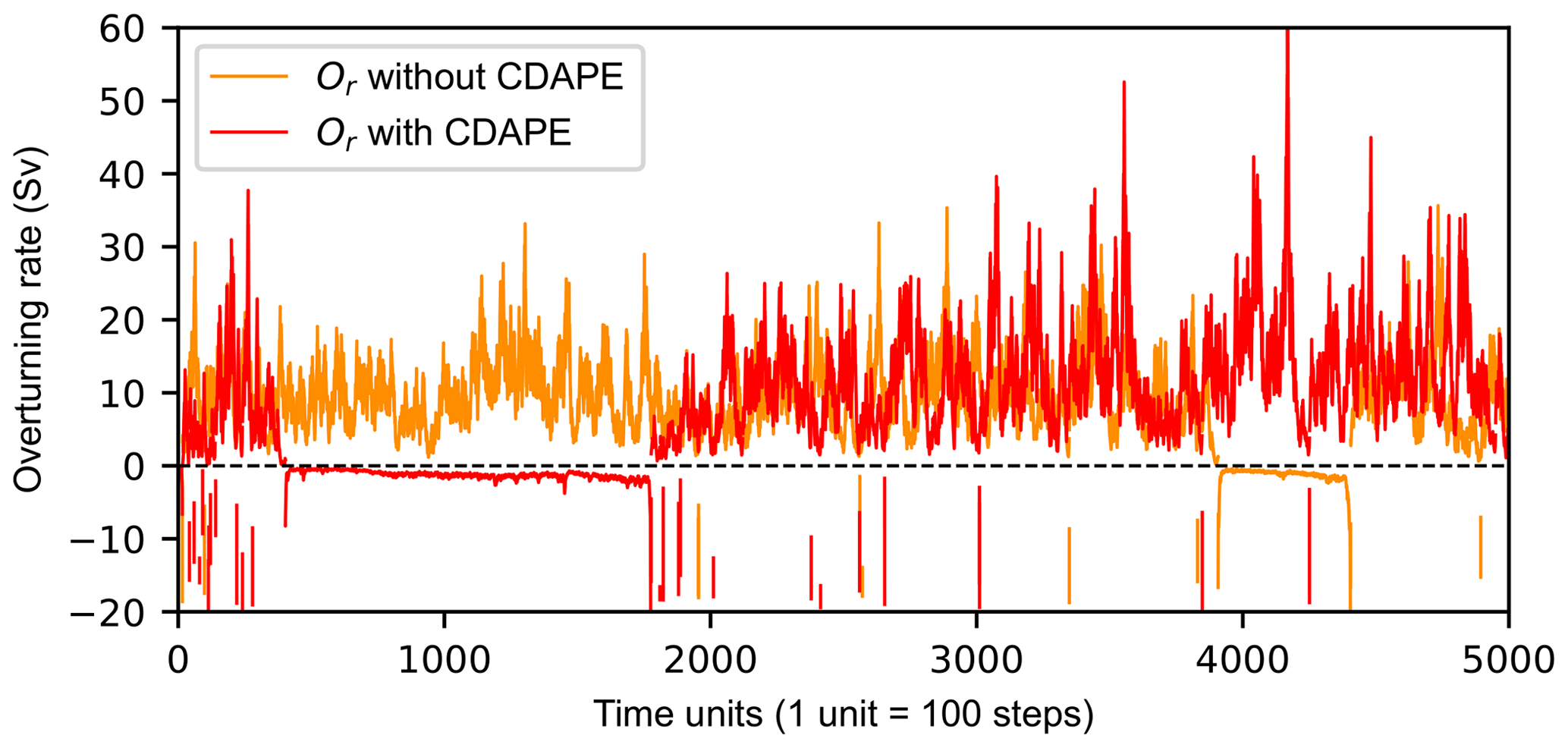
Figure 7 Time series of the overturning rate in one of the ensemble members in the free model control ensemble simulations with (red) or without (orange) data assimilation and parameter estimation, where κ is erroneously guessed as 31.87768. The dashed black line denoting v=0 is a division line between the thermal-mode equilibrium state and the haline-mode equilibrium state.

The five-variable conceptual climate model could simulate the interactions between the atmosphere and ocean, and coupling it with the three-box MOC model could accurately address the main questions in this paper. The transferring of the uncertainty of the MOC3B-5V model is particularly simple and easily understood. With the help of this model, we found that the coupled model parameter estimation with observations can significantly mitigate the model deviations, thus capturing regime transitions of the AMOC. As such, the main outcome of this paper can be more readily demonstrated with this simple model. However, The MOC3B-5V model is just a simple conceptual model, and the model states x₂, w, and η simply conceptually simulate the variation characteristics of the atmosphere and the ocean. Although the transitions of the AMOC are simulated by the MOC3B-5V model, the specific physical meaning of the model is not explicit enough. The method of capturing regime transitions in Sect. 2 is proven to be feasible in the simple model, and the next step is to apply the method to a physics-based MOC box model.

4 Capturing AMOC regime transitions by parameter estimation in a physics-based MOC box model (MOCBM)

4.1 The MOCBM

After proving that it is feasible to capture regime transitions by constraining parameters in an idealized conceptual model, we also use a MOCBM (Tardif et al., 2014; Zhao et al., 2019) with a better physical basis to study the problem of AMOC transition. The MOCBM is a coupled lower-order ocean–atmosphere climate model constructed by Roebber (1995), which reflects the chaotic variability in the atmosphere and the oscillation or multi-equilibria in the ocean (Roebber, 1995; Taboada and Lorenzo, 2005). The atmospheric part of the model is represented by the wave-mean-flow atmospheric circulation model of Lorenz (1984). In contrast to Lorenz's 1963 model describing convection, Lorenz's 1984 model simulates the general atmospheric circulation at mid-latitudes (Lorenz, 1984). The ocean part of the model is represented by another three-box model of the North Atlantic Ocean at mid-latitude (Birchfield, 1989). A schematic illustration of this MOCBM can be found in Fig. 1 of Tardif et al. (2014).

In MOCBM, the model states (vector x) include atmospheric states X, Y, and Z and oceanic states T₁, T₂, T₃, S₁, S_2, and S₃. The governing equations of the atmosphere model are

$$\begin{array}{}\text{(16)}& \begin{array}{rl}& \dot{X}=-\left(Y^{\mathrm{2}}+Z^{\mathrm{2}}\right)-aX+aF,\\ & \dot{Y}=XY-bXZ-Y+G,\\ & \dot{Z}=XZ+bXY-Z,\end{array}\end{array}$$

where X represents the intensity of the westerly wind current, and Y and Z represent the magnitudes of cosine and sine phases of large-scale eddies, respectively. The terms XY and XZ represent the amplification of the eddies through interaction with the westerly current. This amplification is at the expense of the westerly current, which is denoted by the term $-(Y^{\mathrm{2}}+Z^{\mathrm{2}})$. The terms −bXZ and bXY represent the displacement of the eddies by the westerly current, while −aX, −Y, and −Z represent mechanical damping. Finally, F represents the diabatic heating contrasts between the low- and high-latitude ocean, and G represents the longitudinal heating contrast between land and sea.

The simple non-dimensional ordinary differential equations are

$$\begin{array}{}\text{(17)}& \begin{array}{rl}& r_{\mathrm{1}}{\dot{T}}_{\mathrm{1}}={\displaystyle \frac{\mathrm{1}}{\mathrm{2}}}q(T_{\mathrm{2}}-T_{\mathrm{3}})+K_T(T_{A\mathrm{1}}-T_{\mathrm{1}})-K_Z(T_{\mathrm{1}}-T_{\mathrm{3}}),\\ & r_{\mathrm{2}}{\dot{T}}_{\mathrm{2}}={\displaystyle \frac{\mathrm{1}}{\mathrm{2}}}q(T_{\mathrm{3}}-T_{\mathrm{1}})+K_T(T_{A\mathrm{2}}-T_{\mathrm{2}})-K_Z(T_{\mathrm{2}}-T_{\mathrm{3}}),\\ & r_{\mathrm{3}}{\dot{T}}_{\mathrm{3}}={\displaystyle \frac{\mathrm{1}}{\mathrm{2}}}q(T_{\mathrm{1}}-T_{\mathrm{2}})+K_Z(T_{\mathrm{1}}-T_{\mathrm{3}})+K_Z(T_{\mathrm{2}}-T_{\mathrm{3}}),\\ & r_{\mathrm{1}}{\dot{S}}_{\mathrm{1}}={\displaystyle \frac{\mathrm{1}}{\mathrm{2}}}q(S_{\mathrm{2}}-S_{\mathrm{3}})-K_Z(S_{\mathrm{1}}-S_{\mathrm{3}})-Q_{\mathrm{S}},\\ & r_{\mathrm{2}}{\dot{S}}_{\mathrm{2}}={\displaystyle \frac{\mathrm{1}}{\mathrm{2}}}q(S_{\mathrm{3}}-S_{\mathrm{1}})-K_Z(S_{\mathrm{2}}-S_{\mathrm{3}})+Q_{\mathrm{S}},\\ & r_{\mathrm{3}}{\dot{S}}_{\mathrm{3}}={\displaystyle \frac{\mathrm{1}}{\mathrm{2}}}q(S_{\mathrm{1}}-S_{\mathrm{2}})+K_Z(S_{\mathrm{1}}-S_{\mathrm{3}})+K_Z(S_{\mathrm{2}}-S_{\mathrm{3}}),\end{array}\end{array}$$

where K_T represents the coefficient of heat exchange between the ocean and the atmosphere, K_Z represents the coefficient of vertical interaction between the upper ocean and the deep ocean, T_A1 and T_A2 are the air surface temperature, and Q_S is the volume-averaged equivalent salt flux. The non-dimensional variables r₁, r₂ and r₃ are defined as $r_j=V_j/(V_{\mathrm{1}}+V_{\mathrm{2}}+V_{\mathrm{3}}$), where V_j represents the volume of box j. The meridional overturning circulation q satisfies

$$\begin{array}{}\text{(18)}& q=\mathit{\mu }\left[\mathit{\alpha }(T_{\mathrm{2}}-T_{\mathrm{1}})-\mathit{\beta }(S_{\mathrm{2}}-S_{\mathrm{1}})\right],\end{array}$$

where α and β are the thermal and haline expansion coefficients of seawater, respectively, and μ is a proportionality constant.

The coupled interaction between the ocean box model and the atmosphere model is accomplished by the terms F, G, T_A1, T_A2, and Q_s. Superimposing the background value and the variation in a seasonal cycle as well as long-term variation associated with changes in upper ocean temperatures, F and G are defined as

$$\begin{array}{}\text{(19)}& \begin{array}{rl}& F=F_{\mathrm{0}}+F_{\mathrm{1}}\cos \mathit{\omega }t+F_{\mathrm{2}}(T_{\mathrm{2}}-T_{\mathrm{1}}),\\ & G=G_{\mathrm{0}}+G_{\mathrm{1}}\cos \mathit{\omega }t+G_{\mathrm{2}}{T}_{\mathrm{1}},\end{array}\end{array}$$

where F₀, F₁, F₂, G₀, G₁, and G₂ are constants, and ω is the annual frequency. Since X in the atmosphere model is directly related to the temperature, the temperature is defined as

$$\begin{array}{}\text{(20)}& T_{A\mathrm{1}}=T_{A\mathrm{2}}-\mathit{\gamma }X,\end{array}$$

where T_A2 and γ are constants. Finally, the equivalent salt flux is formulated by $Q_{\mathrm{S}}=Q_{\mathrm{runoff}}+{\stackrel{\mathrm{‾}}{Q}}_{\mathrm{WV}}+Q_{\mathrm{WV}}^{\prime }$, where Q_runoff is the runoff into the ocean from the rivers, and ${\stackrel{\mathrm{‾}}{Q}}_{\mathrm{WV}}$ and $Q_{\mathrm{WV}}^{\prime }$ are the mean and transient eddy components of the atmospheric water vapor transport, respectively. Q_runoff and ${\stackrel{\mathrm{‾}}{Q}}_{\mathrm{WV}}$ are assumed to be constant and $Q_{\mathrm{WV}}^{\prime }$ is postulated to be linearly related to the eddy sensible heat flux (Y²+Z²) (Stone and Yao, 1990). Finally, Q_s is obtained as follows:

$$\begin{array}{}\text{(21)}& Q_{\mathrm{S}}=c_{\mathrm{1}}+c_{\mathrm{2}}(Y^{\mathrm{2}}+Z^{\mathrm{2}}),\end{array}$$

where c₁ and c₂ are constants to be determined.

The parameters in this MOCBM are set to (a, b, r₁, r₂, r₃, K_T, K_z, T_A2, α, β, μ, F₀, F₁, F₂, G₀, G₁, G₂, γ) = (0.25, 4.00, 16.495, 5.295, 1.332, 0.35, 0.05276, 1, 9.622 × 10⁻⁵ K⁻¹, 7.755 × 10⁻⁴ psu⁻¹, 4 × 10¹⁰ m³ s⁻¹, 6.65, 2.0, 47.9, −3.60, 1.24, 3.81, 0.06364). As in Roebber (1995), the value of Q_s affects the solution of the thermohaline circulation, and Q_s above a critical value will eventually lead to a complete reversal of the flow. To obtain this critical value of Q_s, the equilibrium solution for the thermohaline circulation is calculated as the value of Q_s varies from 0.5 × 10⁻³ to 4.0 × 10⁻³. As shown in Fig. 8, this critical value is near 2.05 × 10⁻³. Considering the mean and the range of variation of (Y²+Z²), and also referring to the values taken in Roebber (1995) and Tardif et al. (2014), c₁ and c₂ are set here to 1.94 × 10⁻³ and 4.05 × 10⁻⁵, respectively.

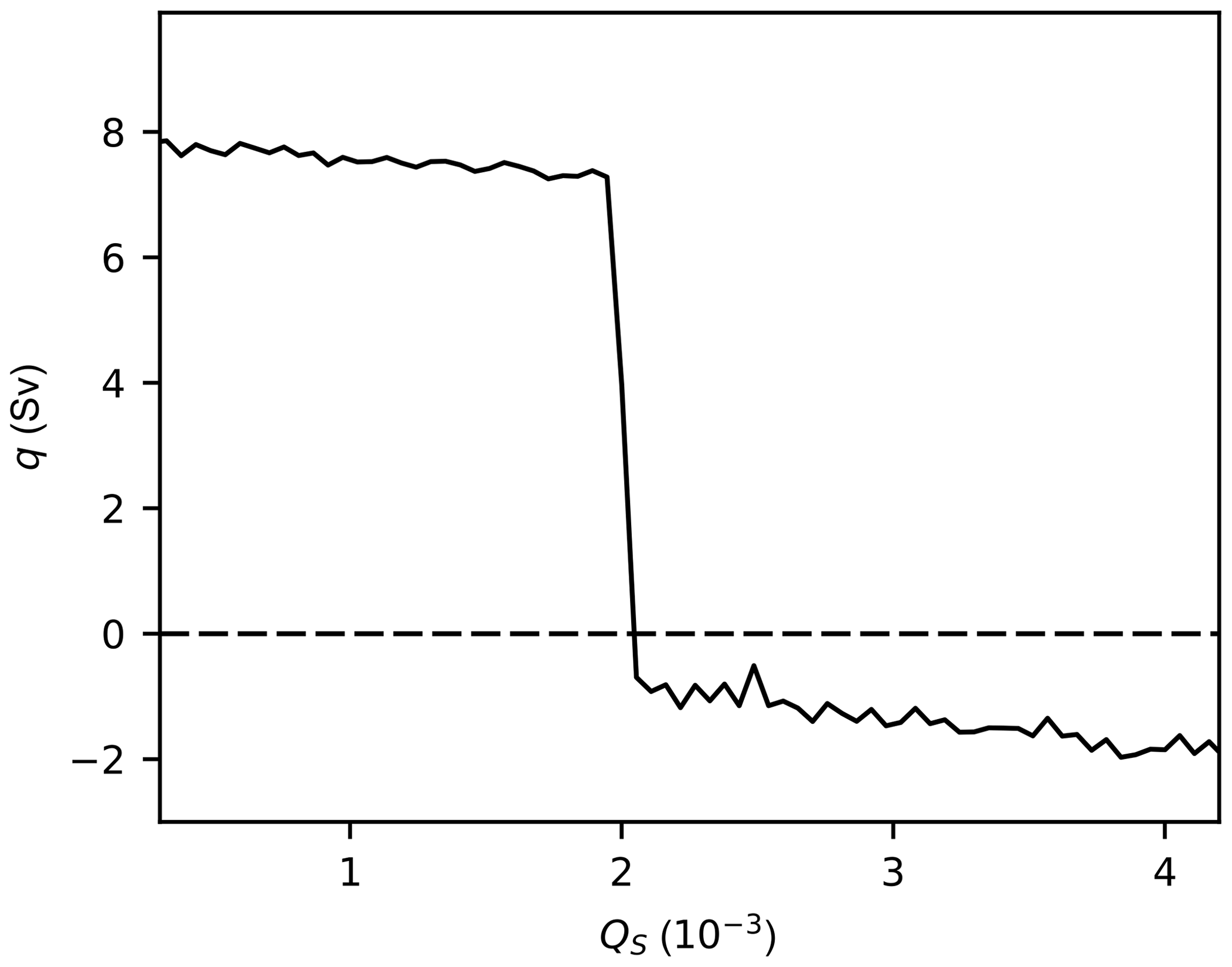
Figure 8 Variation of meridional overturning circulation q in the space of salt flux Q_s. The dashed black line denoting q=0 Sv is a division line between two equilibrium states.

4.2 Parameter estimation with observational information

A twin experimental framework is designed to perform the study of capturing regime transitions using the MOCBM. Using a fourth-order Runge–Kutta time-differencing scheme with a time step of 3 h, the MOCBM is specified with parameter values described above. The truth model is spun up for an initial 10⁵ years starting from an initial value of q equal to 15 Sv. Then, another 60 000 years are run forward to produce the “truth” states. The states of the atmosphere and the temperature and salinity of the surface ocean are considered the variables to be observed. The white noise is added to the “truth” states, and the standard deviations of the observation errors are set to 0.1 for X, Y, and Z, 0.5 K for T₁ and T₂, and 0.1 psu for S₁ and S₂. The “observations” are eventually obtained by sampling these variables at a frequency of 1 year. In the twin experimental framework, the assimilation model is similar to the truth model, except that parameter γ in the box model is assumed to be incorrectly estimated, with an error that is 10 % greater than the standard value 0.06364. Thus, the mean value of all parameters from the 20 assimilation models is 0.070004, and their standard deviation is 10 % of the standard value. The parameters in the atmosphere model or in the ocean model could be selected for parameter estimation to address the points in this paper. Given that we have experimented with the parameter in the atmosphere model before, here we show the experiment with the parameter of the ocean model. Again, the parameter being estimated is based on the model sensitivities regarding all parameters in the box model (Zhao et al., 2019).

Figure 9 shows the time series of meridional overturning circulation q, where the positive and negative aspects of q reflect the reversed circulation, which represents the transition between two different states. The simulation results of the 20 assimilation models (orange line in Fig. 9a) are different, and they all have significant errors with the results from the truth model (red line). Then, the “observations” from the truth model are used to adjust the model states (Fig. 9b) as well as to further constrain the parameter γ (Fig. 9c). Figure 9b shows the time series of the MOC value in the “truth” simulation (red lines) and in the free model control ensemble simulations with only data assimilation. Due to the existence of parameter error, inaccurate analyses are obtained when only data assimilation was performed without parameter estimation. The results of data assimilation and parameter estimation are shown in Fig. 9c, where the simulation results of the 20 assimilation models (orange lines) are constrained by “observations”, and the more accurate reconstructed transition path (red lines) is obtained. Since the behaviors of the MOCBM and MOC3B-5V models are very similar, the figures corresponding to Figs. 6 and 7 are not shown here.

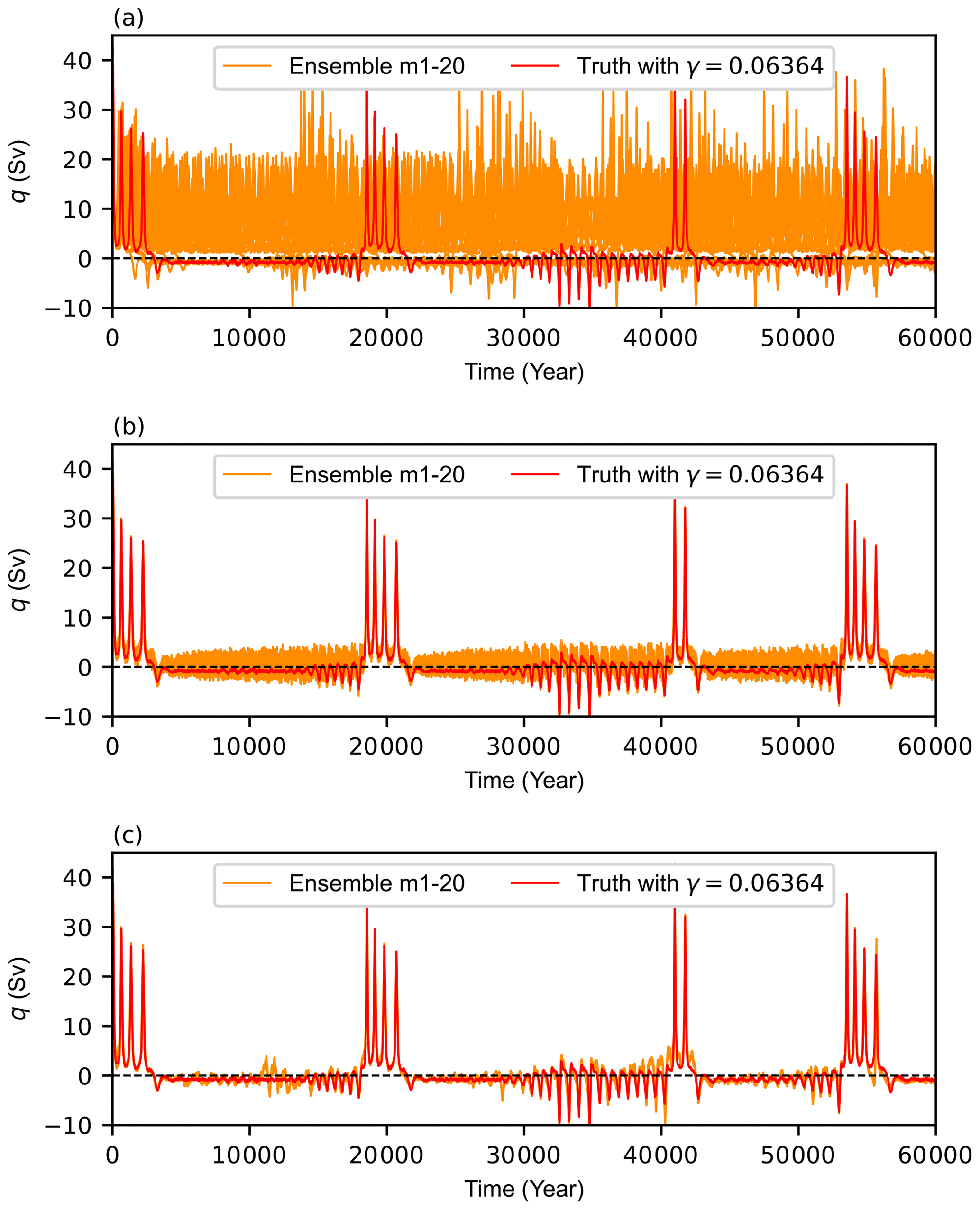
Figure 9 Time series of the meridional overturning circulation q in the “truth” simulation with γ=0.06364 (red) and the individual ensemble members (orange) in the free model control ensemble simulations (a) without data assimilation and parameter estimation, (b) with data assimilation or (c) with data assimilation and parameter estimation using erroneously guessed γ values with a Gaussian perturbation that has a mean value of 0.070004 and a standard deviation of 10 % times the standard value. The dashed black line denoting q=0 is a division line between two equilibrium states.

The box model in the MOCBM is based on the classical approach of adopting a buoyancy constraint, and the circulation is regulated by the surface buoyancy difference, implying that surface thermohaline forcing drives the AMOC (Birchfield, 1989). In contrast, for the box model in the MOC3B-5V model, the constraint is based on mechanical energy sustaining diapycnal mixing, and the circulation is maintained by mechanical energy from wind stress and tides (Shen et al., 2011). The AMOC is driven differently in the two box models. Compared with the buoyancy constraint (MOCBM), the energy constraint (MOC3B-5V) can offer a significant advantage in rational interpretations of the transitions between the thermal and haline modes (Guan and Huang, 2008). Compared to the MOC3B-5V model, the MOCBM is more explicit in physical meaning, which is mainly reflected in the meaning of the model states. The meaning of the state variables in the atmospheric part of the MOCBM is more explicit, such as X for the westerly wind current and Y and Z for large-scale eddies. The MOC3B-5V model, however, only describes the chaotic characteristic of the atmosphere starting from a simple heating disturbance problem. It further describes the basic variation characteristic of the ocean by the coupled interaction between the atmosphere and the ocean. Besides, the coupling of ocean and atmosphere in the MOCBM is sufficiently accomplished by several variables such as F, T_A1, and Q_s. The MOC3B-5V model and the MOCBM, although both are simple models, can reveal the characteristic of AMOC multi-equilibria and thus can be used to test the feasibility of the methodology in Sect. 2. By constraining the model parameters with observations, both models result in capturing regime transitions of the AMOC.

5 Summary and discussions

A method for combining the general AMOC simulation model with ensemble Kalman filtering is designed to form a CDAPE system. Given that the discrepancy exists between the influencing factors of the AMOC in the real world and the corresponding parameters of models, parameter estimation is used to estimate the model parameters. Using the CDAPE system, within a “twin” experiment framework, 20 assimilation models are set with an incorrectly estimated parameter, while a model representing the “truth” uses the parameters as the standard values. The assimilation models simulate 20 different transition paths between AMOC states with disturbing parameters. The observational information from the “truth” is assimilated into the assimilation models, and the transition path of the AMOC is optimized by parameter estimation, so that regime transitions of the AMOC are captured correctly. Our results suggest that, guided by estimation theory, appropriately constraining coupled model parameters with observed data can make a climate model capture regime transitions of the AMOC. The research methodology is applied to simple climate models that can simulate AMOC multi-equilibria. The first model in this study provides conceptual proof that the methodology is feasible, and the second model with more explicit physical meaning provides further demonstration through simulation results.

A simple model that consists of a three-box ocean model and a five-variable climate model (the MOC3B-5V model) has been developed to simulate the basic characteristic of the AMOC that transits between different equilibrium states. The parameters in the three-box model are linked to the atmospheric variables, the upper ocean variable, and the deep ocean variable in the five-variable model to construct energy constraint, wind-driven circulation, and freshwater flux, which dynamically change within a reasonable range. By projecting observational information of model states to the parameters, the AMOC regime transitions simulated by the model are much closer to reality. It has to be noted that after the change in the three-box model from the stable haline mode to the stable thermal mode, a catastrophic change occurs in the system, which results in the disappearance of the stable haline mode (Guan and Huang, 2008). It is impossible to change the state from the thermal mode to the haline mode by changing parameters. Therefore, to adjust the transition between the thermal mode and the haline mode, additional atmospheric forcing (additional freshwater flux from the atmosphere) is added to the two boxes that have contact with the atmosphere. The effect of this forcing is small and does not affect the overall balance of the model. Although we acknowledge that the effect of additional forcing still needs to be further investigated, the disappearance of the haline mode is not addressed in this study, so that we may focus on capturing regime transitions by observation-constrained model parameters. It is important to emphasize that the simple conceptual model is not attempting to simulate a specific oceanic and atmospheric physical process, but rather the opposite: our objective is to explore whether the error between models and reality in terms of the AMOC transition can be reduced by incorporating observational information into the model parameters.

The MOCBM (Roebber, 1995) with clearer physical meaning is used in this study. Since the circulation is driven only by the meridional gradients of the upper ocean temperature and salinity in the buoyancy-constraint MOCBM, AMOC regime transitions can be captured to some extent when the upper ocean temperature and salinity are directly adjusted by data assimilation only, but the simulation results are not accurate enough. In this simple model, since the data assimilation has worked well, the contribution of parameter estimation is relatively small but still indispensable. The AMOC regime transitions are captured more accurately by parameter estimation. The degree of contributions of data assimilation or parameter estimation to the optimization of simulation results is different in these two models. Compared with the MOCBM, the energy-constraint MOC3B-5V model is more representative of the role of parameter estimation because the circulation is maintained by mechanical energy. When leaving out the parameter estimation steps and constraining the model states only by data assimilation, the accuracy of state estimation is not high due to the existence of parameter errors. Given the fact that the circulation is driven in a more complex way in the real world, this simple model study only provides a conceptual understanding and guideline for more complex real systems such as a coupled general circulation model (CGCM). Although both the MOCBM and the MOC3B-5V model are simple idealized hemispheric models, our concerns can be illustrated more clearly through them. Our effort here is to make the AMOC multiple equilibrium states from model simulations better reflect the features in reality. Our focus is on adjusting the model parameters by sampling the observations so that the simulation of the model is closer to the truth in the feature of regime transitions. The conceptual model, albeit simple, has demonstrated the importance of data assimilation and parameter estimation. It is hoped that such a simple model study on AMOC transition will inspire the hypotheses and the optimization of parameters in CGCMs. Taking a study by Ashkenazy and Tziperman (2007) as an example, to understand the ocean general circulation model results, they constructed a simple three-box model to understand the behavior of the thermohaline circulation in more realistic parameter regimes (Ashkenazy and Tziperman, 2007).

We have already captured regime transitions of the AMOC in a conceptual model as well as in a simple model with clearer physical meaning and will apply this method to more complex real systems such as CGCMs. The characteristic of AMOC multi-equilibria has been simulated in box models (e.g., Stommel, 1961; Rooth, 1982; Welander, 1986; Birchfield, 1989), ocean circulation models (e.g., Marotzke and Willebrand, 1991), and coupled ocean–atmosphere models (e.g., Manabe and Stouffer, 1988). However, it should also be noted that AMOC multiple equilibria have not been directly simulated by some CGCMs. Tremendous research efforts thus have been put into tackling this issue. One focus was on the CGCM presentation of Stommel's salt advection feedback (Rahmstorf, 1996). It has been suggested that this feedback is distorted in CGCMs due to salinity biases (Huisman et al., 2010; Jackson, 2013; Liu et al., 2017). Another argument is on ocean eddies. It has also been suggested that CGCMs with an eddy-permitting ocean allow for a simulation of AMOC multiple equilibria (Jackson and Wood, 2018) since ocean eddies modify the overall freshwater balance (Mecking et al., 2016). In follow-up studies, we will explore the contribution of a CDAPE system to AMOC multi-equilibrium using different resolutions, ranging from a coarse-resolution CGCM with the ability to simulate AMOC multi-equilibrium characteristic and eventually to a high-resolution and more realistic Earth system model. In a recent study, two types of AMOC transitions were described, with a temporary cessation of the downwelling (called an F-type transition) or a full collapse of the AMOC (called an S-type transition), and the F-type transitions might have been found in the direct observation (Castellana et al., 2019; Castellana and Dijkstra, 2020). The general methodology of this study could be used for both S-type transition and F-type transition. The S-type transition with centurial and millennial timescales could use observations from paleoclimate records, and the methodology can be applied to paleoclimate models for capturing AMOC regime transitions. In the current climate system, the F-type transition with very high transition probabilities on multi-decadal timescales (Castellana et al., 2019; Castellana and Dijkstra, 2020) could use direct observations from RAPID or indirect observations from satellites or the ARGO program.

Although the observation-constrained model simulates the transition between different equilibrium states of the AMOC, this study only serves as the first step of capturing regime transitions, and many challenges still exist. First, the deviations of AMOC transition paths simulated in different models are caused by not only parameter errors, but also mismatches between real physical processes and model simulations (Zhang et al., 2012). Therefore, the performance of parameter estimation still needs further experimentation with more realistic models. Second, the mechanism of AMOC transition needs further investigation. The effect of stochastic forcing has been taken into account in previous work. Cessi (1994) studied the transition from one equilibrium to another in a modified Stommel model, and she found that the transition could occur under stochastic white-noise forcing. In our study, the transition phenomenon of the AMOC is ultimately affected by the model parameters. Usually, traditional state estimation with data assimilation has limited usage in detecting the mechanism. Here, we aim at constraining the model parameters through utilization of observational information, which eventually results in a more realistic model behavior in terms of the AMOC transitions. A future effort is needed on how the effect of the stochastic component will manifest in the AMOC system. Third, Aksoy et al. (2006b) proposed a spatial updating technique that recovers the globally uniform parameter value using a spatial average of the entire spatially varying parameter field. Wu et al. (2012, 2013) explored the impact of the geographic dependence of the observing system on the parameters. The adjustment of the parameters is based on the spatial distribution of the model state sensitivity to parameters. Liu et al. (2014a, b) proposed the adaptive spatial average method that obtains the final global uniform posterior parameter based on spatially varying posterior estimated parameter values. In this study, considering that the simple box models are used as a first step to explore AMOC transitions, it is more appropriate to use the identity model. The impact of geographic-dependent parameter optimization on climate estimation and prediction can be considered in future studies for complex systems such as CGCMs.

Besides, in the study of two simple models, the observational information, which is used for data assimilation and parameter estimation, only comes from the atmosphere and surface ocean. In the real Earth system, the flow of seawater located in the deep ocean is an important part of the AMOC, and its measurement is difficult. The changes in each component of the AMOC will affect the entire circulation. AMOC reconstruction heavily relies on comprehensive observational data. In the future, with the improvement of the Earth-observing system, the coupled climate system model will be improved continuously, and the results of numerical simulation will have a higher credibility. These could lead to significant improvement of the reanalysis and prediction of the AMOC.