the Creative Commons Attribution 4.0 License.
the Creative Commons Attribution 4.0 License.
 | 19 Jan 2021
Ordering of trajectories reveals hierarchical finite-time coherent sets in Lagrangian particle data: detecting Agulhas rings in the South Atlantic Ocean
Christian Kehl
Henk A. Dijkstra
Erik van Sebille
The detection of finite-time coherent particle sets in Lagrangian trajectory data, using data-clustering techniques, is an active research field at the moment. Yet, the clustering methods mostly employed so far have been based on graph partitioning, which assigns each trajectory to a cluster, i.e. there is no concept of noisy, incoherent trajectories. This is problematic for applications in the ocean, where many small, coherent eddies are present in a large, mostly noisy fluid flow. Here, for the first time in this context, we use the density-based clustering algorithm of OPTICS (ordering points to identify the clustering structure; Ankerst et al., 1999) to detect finite-time coherent particle sets in Lagrangian trajectory data. Different from partition-based clustering methods, derived clustering results contain a concept of noise, such that not every trajectory needs to be part of a cluster. OPTICS also has a major advantage compared to the previously used density-based spatial clustering of applications with noise (DBSCAN) method, as it can detect clusters of varying density. The resulting clusters have an intrinsically hierarchical structure, which allows one to detect coherent trajectory sets at different spatial scales at once. We apply OPTICS directly to Lagrangian trajectory data in the Bickley jet model flow and successfully detect the expected vortices and the jet. The resulting clustering separates the vortices and the jet from background noise, with an imprint of the hierarchical clustering structure of coherent, small-scale vortices in a coherent, large-scale background flow. We then apply our method to a set of virtual trajectories released in the eastern South Atlantic Ocean in an eddying ocean model and successfully detect Agulhas rings. We illustrate the difference between our approach and partition-based k-means clustering using a 2D embedding of the trajectories derived from classical multidimensional scaling. We also show how OPTICS can be applied to the spectral embedding of a trajectory-based network to overcome the problems of k-means spectral clustering in detecting Agulhas rings.
- Article
(9929 KB) - Full-text XML
- BibTeX
- EndNote


Understanding the transport of tracers in the ocean is an important topic in oceanography. Despite large-scale transport features of the mean flow, on smaller scales, mesoscale eddies and jets play an important role for tracer transport (van Sebille et al., 2020). Such eddies can capture large amounts of a tracer and, while transported in a background flow, redistribute them in the ocean. Eddies have been shown to play an important role in the accumulation of plastic (Brach et al., 2018) and the transport of heat and salt (Dong et al., 2014). To quantify the effects of eddies on tracer transport in the ocean, it is necessary to develop methods that are able to detect and track them. Many methods exist to detect such finite-time coherent sets of fluid parcels based on different mathematical or heuristic principles (Hadjighasem et al., 2017). The term finite-time coherent set is based on the work of Froyland et al. (2010) and is, in our context, defined as a set of particles that, in a sense, stay specifically close to each other along their entire trajectories. Here, for the first time in this context, we make use of the density-based clustering algorithm OPTICS (ordering points to identify the clustering structure; Ankerst et al., 1999) to detect finite-time coherent sets in Lagrangian trajectory data.
The detection of coherent Lagrangian vortices using abstract embeddings of Lagrangian trajectories together with data-clustering techniques has received significant attention in the recent literature (Froyland and Padberg-Gehle, 2015; Hadjighasem et al., 2016; Padberg-Gehle and Schneide, 2017; Banisch and Koltai, 2017; Schneide et al., 2018; Froyland and Junge, 2018; Froyland et al., 2019). Using embedded trajectories for the detection of finite-time coherent sets is interesting as it allows one to use sparse trajectory data, and it can, in principle, be applied to ocean drifter trajectories, as demonstrated by Froyland and Padberg-Gehle (2015) and Banisch and Koltai (2017) for the detection of the five ocean basins. Yet, most of these methods cluster trajectory data with graph partitioning, which does not incorporate the difference between coherent, clustered trajectories and noisy trajectories that should not belong to any cluster. Graph partitioning has been shown to work in situations where the finite-time coherent sets are not too small compared to the fluid domain (Froyland and Padberg-Gehle, 2015; Hadjighasem et al., 2016; Padberg-Gehle and Schneide, 2017; Banisch and Koltai, 2017; Froyland and Junge, 2018). For applications to Lagrangian trajectory data sets on basin-scale ocean domains, where multiple small-scale coherent sets (eddies) coexist with noisy trajectories in the background, graph partitioning is, however, likely to fail. Similar observations were made by Froyland et al. (2019) for the partition-based clustering approaches based on transfer and dynamic Laplace operators (Froyland and Junge, 2018). Although some attempts have been made to accommodate such concepts in hard partitioning, e.g. by incorporating one additional cluster corresponding to noise (Hadjighasem et al., 2016), this approach is likely to fail for large ocean domains, as discussed by Froyland et al. (2019) and shown in Sect. 4 of this paper. Froyland et al. (2019) have developed a special form of trajectory embedding, based on sparse eigenbasis decomposition, given the eigenvectors of transfer operators and dynamic Laplacians. By superposing different sparse eigenvectors, they successfully separate coherent vortices from unclustered background noise.
Motivated by the results Froyland et al. (2019) obtained by developing a new form of trajectory embedding, we here explore the potential of another clustering algorithm to overcome the inherent problems of partition-based clustering. We use the density-based clustering method of OPTICS, developed by Ankerst et al. (1999), to detect finite-time coherent sets in large ocean domains, using a very simple choice of embedding (see Sect. 3.2.1). Density-based clustering aims to detect groups of data points that are close to each other, i.e. regions with high data density. Our data points correspond to entire trajectories, and groups of trajectories staying close to each other over a certain time interval correspond to such regions of high point density. Different from partition-based methods such as k-means or fuzzy-c-means, OPTICS does not require one to fix the number of clusters beforehand. Furthermore, density-based clustering has an intrinsic notion of a noisy data point – a point does not belong to any cluster (i.e. a finite-time coherent set) if it is not part of a dense region. A more detailed comparison of the method presented here to existing related methods can be found in Sect. 3.4.
Another desirable property of the OPTICS algorithm is its ability to capture coherence hierarchies. In the ocean, coherent sets of trajectories naturally come with a notion of such a hierarchy. For example, the surface flow in the North Atlantic Ocean can be seen as approximately coherent (Froyland et al., 2014), while mesoscale eddies and jets are also finite-time coherent sets of trajectories at smaller scales within the North Atlantic Ocean. Froyland et al. (2019) show how their leading eigenvectors resolve coherent sets at large scales, while small-scale results can be obtained with a sparse eigenbasis approximation of a set of eigenvectors. Similarly, clustering results obtained from OPTICS is typically hierarchical. The main result of OPTICS, i.e. the reachability plot, provides this hierarchical information in a simple 1D graph.
In Sect. 4, we first show how OPTICS detects finite-time coherent sets at different scales for the Bickley jet model flow (also discussed, e.g., by Hadjighasem et al., 2017) and successfully detects the six coherent vortices and the jet as the steepest valleys in the reachability plot. The general structure of the reachability plot also reveals the large-scale finite-time coherent sets, i.e. the northern and southern parts of the model flow, separated by the jet. We then apply our method to Lagrangian particle trajectories released in the eastern South Atlantic Ocean, where large rings detach from the Agulhas Current (e.g. Schouten et al., 2000). We detect several Agulhas rings and, on the larger scale, also separate the eastward- and westward-moving branches of the South Atlantic subtropical gyre. While the traditional approach to studying Agulhas rings is based on sea surface height analysis (see, e.g., Dencausse et al., 2010), several methods based on virtual Lagrangian trajectories have been applied to Agulhas ring detection before (Haller and Beron-Vera, 2013; Beron-Vera et al., 2013; Froyland et al., 2015; Hadjighasem et al., 2016; Tarshish et al., 2018). Our method is different from these approaches in that it is directly applicable to a trajectory data set, i.e. without much preprocessing of the data. As the OPTICS algorithm is readily available in the scikit-learn library in Python, the detection of finite-time coherent sets can be done without much effort and with only a few lines of code. A further difference is the mentioned intrinsic notion of coherence hierarchy, which allows for simultaneous analysis of trajectory data at different scales. While we mainly focus on the direct embedding of trajectories in an abstract, high-dimensional Euclidean space, we also show in Appendix C that OPTICS can be used to overcome the limits of k-means clustering in the context of spectral clustering of the trajectory-based network of Padberg-Gehle and Schneide (2017).
2.1 Quasi-periodically perturbed Bickley jet
We apply our method to a model system that has been used frequently in studies to detect finite-time coherent sets (Hadjighasem et al., 2017; Padberg-Gehle and Schneide, 2017; Hadjighasem et al., 2016; Banisch and Koltai, 2017; Froyland and Junge, 2018). The velocity field of the quasi-periodically perturbed Bickley jet (Bickley, 1937; del Castillo-Negrete and Morrison, 1993) is defined by a stream function , i.e. and , with consisting of a stationary eastward background flow as follows:
and a time-dependent perturbation, as follows:
where Re(z) denotes the real part of the complex number z. We use the same parameter values as Hadjighasem et al. (2017), with U=62.66 m/s the characteristic velocity of the zonal background flow, and L=1770 km. The parameters in Eq. (2) are given by and , with ϵ1=0.075, ϵ2=0.4, ϵ3=0.3, c1=0.1446U, c2=0.205U and c3=0.461U. The domain of interest is , 3000 km], where r0=6371 km is the radius of the Earth, and the left and right edges of Ω are identified, i.e. the flow is periodic in the x direction with period πr0. Similar to Banisch and Koltai (2017), we seed the domain with an initial number of 12 000 particles on a uniform 200×60 grid. For this choice, the initial particle spacing is slightly above 100 km in both directions. We compute the trajectories for 40 d with a time step of 1 s using the SciPy integrate package. We output the trajectories every day, i.e. we have T=41 data points in time for each trajectory.
2.2 Agulhas rings in the South Atlantic
To test the OPTICS algorithm with a more realistic ocean flow, we simulate surface particle trajectories in a strongly eddying ocean model. Surface velocities are derived from a Nucleus for European Modelling of the Ocean (NEMO) ORCA-N006 run (Madec, 2008), which has a horizontal resolution of and velocity output for every 5 d. The model is forced by reanalysis and the observed data of wind, heat and freshwater fluxes (Dussin et al., 2016), i.e. the currents do not only contain the geostrophic component, as is the case in altimetry-derived currents (Beron-Vera et al., 2013; Froyland et al., 2019). For the advection of virtual particles, we use version 1.11 of the open source Parcels framework (Lange and van Sebille, 2017, see http://oceanparcels.org/, last access: 2 January 2021). The 2D surface current velocity is interpolated in space and time with the C-grid interpolation scheme of Delandmeter and van Sebille (2019), using a fourth-order Runge–Kutta method with a time step of 10 min. We initially distribute particles uniformly in the ocean on the vertices of a grid in the domain (30∘ W, 20∘ E) × (40∘ S, 20 ∘ S), which corresponds to a total number of 23 821 particles. At 30∘ S, a spacing of 0.2∘ corresponds to roughly 20 km. The particles start on 5 January 2000 and are advected for 2 years. We output the trajectories with a time interval of 5 d. We only use the first 100 d as data to detect the finite-time coherent sets, i.e. we have T=21 data points for each trajectory, but also look at later times to see how long the rings need to disperse. We provide the used trajectory data for the Agulhas flow as a NumPy file on Zenodo (Wichmann, 2020b).
3.1 Detecting coherent structures in Lagrangian trajectory data
For N trajectories of dimension D and length T, the trajectory information can be stored in a data matrix , where each row results from a particle trajectory by concatenating the different spatial dimensions. The analysis of the trajectory data to detect the finite-time coherent sets of trajectories (Froyland and Padberg-Gehle, 2015; Banisch and Koltai, 2017; Hadjighasem et al., 2016; Padberg-Gehle and Schneide, 2017; Schneide et al., 2018; Froyland and Junge, 2018; Wichmann et al., 2020) can be split into the following two essential steps:
-
Step 1. Embedding of the trajectories in an abstract (metric) space, i.e. , where M≤DT. If one uses a dimensionality reduction method, then M<DT.
-
Step 2. Clustering of the embedded data with a clustering algorithm.
The embedding is necessary to represent the trajectories as points in a metric space. Different options for embedding the trajectories exist, e.g. a direct embedding of the data points along the trajectories (Froyland and Padberg-Gehle, 2015) or embeddings based on the eigenvectors derived from networks that are defined by physically motivated trajectory similarities (Banisch and Koltai, 2017; Padberg-Gehle and Schneide, 2017; Banisch and Koltai, 2017; Froyland and Junge, 2018). Once an embedding of each trajectory as a point in a metric (typically Euclidean) space is established, one can apply a clustering algorithm. Roughly speaking, clustering algorithms try to identify groups of points that are close to each other as a cluster. Partition-based clustering methods divide the entire data set into a (typically fixed) number of K clusters, such that each data point belongs to a cluster. The most popular method in this category is the k-means algorithm, which tries to find a given number of K clusters such that the sum of the pairwise squared distances of points within a cluster is minimized. Other clustering algorithms contain a concept of noisy data, i.e. data points that do not belong to any cluster or belong to a cluster only with a certain probability. Examples of the former case are density-based spatial clustering of applications with noise (DBSCAN; Ester et al., 1996), as discussed by Schneide et al. (2018) in the fluid dynamics context, and the OPTICS (Ankerst et al., 1999) algorithm presented here. For the latter case, the most popular method is fuzzy-c-means clustering, as discussed by Froyland and Padberg-Gehle (2015) in the context of finite-time coherent sets.
Figure 1 shows a few possible options for trajectory embedding and clustering that have partially been explored before (see the footnotes in the figure for the combinations used in related studies). For a given trajectory data set, one can, in principle, apply an arbitrary combination of embedding and clustering methods. Only a few of the different combinations have been explored so far, and many more options for embedding and clustering (like those shown in Fig. 1) exist. It is important to note that a good choice of embedding and clustering might well depend on the specific problem at hand, and there might be no combination that performs well for all possible situations.
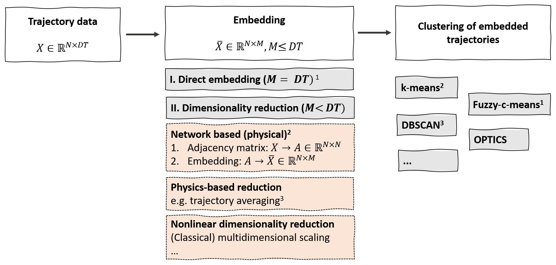
Figure 1Different steps for detecting coherent trajectories in Lagrangian data with trajectory clustering. The figure is nonexhaustive, and many more options for embedding and clustering exist. Footnotes: 1 Froyland and Padberg-Gehle (2015). 2 Hadjighasem et al. (2016), Padberg-Gehle and Schneide (2017) and Banisch and Koltai (2017) all define networks with spectral embedding and subsequent k-means clustering. Froyland et al. (2019) define spectral embeddings as being on dynamic Laplacian and transfer operators. 3 Schneide et al. (2018).
Most of the studies that use clustering techniques to detect finite-time coherent sets have focused on developing new forms of trajectory embeddings. For example, Hadjighasem et al. (2016), Padberg-Gehle and Schneide (2017), Banisch and Koltai (2017) and Froyland and Junge (2018) all use different forms of spectral embeddings together with k-means clustering. Froyland et al. (2019) have developed a powerful form of embedding based on a sparse eigenbasis approximation. Here, we focus on the clustering step in Fig. 1 and propose the OPTICS clustering algorithm in the fluid dynamics context. We test the algorithm for the following three different kinds of embeddings:
- E1.
A direct embedding of the trajectory data in a high-dimensional Euclidean space, i.e. M=DT (see Sect. 3.2.1).
- E2.
A reduction in the trajectory data to a 2D embedding space, using classical multidimensional scaling (MDS; see Sect. 3.2.2). This is mainly to visualize the difference from partition-based k-means clustering.
- E3.
A spectral embedding of the network proposed by Padberg-Gehle and Schneide (2017).
In the following sections, we explain in detail the embeddings of E1 and E2 and the OPTICS algorithm. We introduce the network embedding of E3 together with the corresponding results in Appendix C.
3.2 Trajectory embedding
3.2.1 Direct embedding
The direct embedding of each trajectory in ℝDT is the most straightforward embedding as it requires no further preprocessing of the trajectory data. For simplicity, assume we are given a set of N trajectories in a 3D space, i.e. , where and . We then simply define the embedding of trajectory i in the abstract 3T-dimensional space as follows:
and impose an Euclidean metric in ℝ3T to measure distances between the different embedded trajectories. The resulting embedded data matrix is then simply given by the vertical concatenation of the different embedding vectors. This kind of embedding was also explored by Froyland and Padberg-Gehle (2015), together with a fuzzy-c-means clustering. Intuitively, if two trajectories i and j belong to the same finite-time coherent set, the corresponding particles follow very similar pathways, i.e. the Euclidean distance of the embedding vectors is expected to be small. On the other hand, a particle i that belongs to a coherent set is expected to have a larger distance to a particle j that is not part of the set. In other words, groups of particles that form a finite-time coherent set are dense in the embedding space. This motivates the use of a density-based clustering algorithm to detect finite-time coherent sets.
To take into account the πr0 periodicity in the x direction of the Bickley jet flow, we first put the individual 2D data points on the surface of a cylinder with radius r0∕2 in ℝ3 and interpret the resulting trajectories in a 3D Euclidean space. The resulting data matrix is , with N=12 000 and T=41. For the Agulhas particles, we put the single data points on the Earth's surface in a 3D Euclidean embedding space by the standard coordinate transformation of spherical to Euclidean coordinates. The resulting data matrix is thus , with N=23 821 and T=21.
3.2.2 Dimensionality reduction with classical multidimensional scaling
To develop an intuition for what the OPTICS algorithm does, and the differences to k-means, we wish to visualize the data structure in the plane. For this visualization, it is necessary to reduce the embedding dimension of each trajectory from 3T to two in such a way that the density structure, and hence the individual Euclidean distances between embedded trajectories (see Eq. 3), are preserved. We do so through a common method of nonlinear dimensionality reduction, called classical multidimensional scaling (MDS; see, e.g., chap. 10.3 of Fouss et al., 2016). Classical MDS tries to find an embedding of the high-dimensional data points in a low-dimensional space such that the pairwise distances are approximately preserved. Similar to a principal component analysis, classical MDS makes use of the eigenvectors corresponding to the largest eigenvalues of a kernel matrix, which is, in this case, defined by the following:
where is a matrix containing all squared distances between the points, and H is the centring matrix with , where δij denotes the Kronecker delta. The matrix B in Eq. (4) is called the centred inner product matrix. If is the matrix of inner products of the embedded data points, i.e. with Euclidean scalar product, then B can be obtained by removing the mean of all rows and columns of (see chap. 10.3 of Fouss et al., 2016). An embedding of the data points using the eigenvectors corresponding to the leading nonnegative eigenvalues of B in Eq. (4) ensures that one captures the main variance of the (squared) distance structure, similar to a principal component analysis.
We compute Δ2 with the Euclidean embedding described in Sect. 3.2.1 and restrict ourselves to the first 2D to visualize the data structure in the plane, i.e. the embedding is defined by the following:
where Bwj=λjwj, and for all . This choice of embedding ensures that the main variance of the data points is captured, and we therefore also expect to capture the main structure in terms of data density. For large particle sets, however, computing the spectrum of B in Eq. (4) is computationally not feasible as the matrix B is dense and computing the spectrum scales with O(N3). We apply classical MDS to the 12 000 particles of the Bickley jet model flow and a random selection of the equal number of particles for the Agulhas flow. In our context, the method is most useful for visualization purposes as it provides a good 2D approximation of the point distances, i.e. also the density structure of the embedded trajectories.
3.3 Clustering with OPTICS
The detection of dense accumulations of points that are separated from each other by non-dense regions (noise) is the main goal of density-based clustering. We use the OPTICS algorithm by Ankerst et al. (1999) to detect these regions. The OPTICS algorithm can be seen as an extension of DBSCAN (Ester et al., 1996). As we have no prior information on the density structure of the embedded nodes, we set the generating distance of OPTICS to infinity, and our presentation here is limited to this case. The general OPTICS algorithm with finite generating distance is computationally more efficient and slightly more complicated, and we refer to Ankerst et al. (1999) for more details.
For δ∈ℝ, the δ neighbourhood of a point p∈ℝM is defined as the M-dimensional ball of radius δ around p. We define Mδ(p) as the number of points that is in the δ neighbourhood of p, including p itself. OPTICS requires one parameter, i.e. an integer smin (called MinPts by Ankerst et al., 1999), to define the core distance of a point p as follows:
The core distance is simply the minimum radius of a ball around p, such that the ball contains smin points. Note that the generating distance that we set to infinity is a maximum cut-off distance for the computation of the core distance in Eq. (6), beyond which the core distance is not defined. As we do not have an intuition for a good value of such a cut-off, we remove it by setting it to infinity.
The ordering of the points is based on the reachability distance of a point p with regards to another point q and is defined as follows:
where , in our case, denotes the Euclidean distance between p and q. The ordering of points is then constructed with the following scheme:
-
Step 1. Pick a point p1. This is the first point in the order, and it is arbitrary.
-
Step 2. Compute the core distance c(p1) of p1.
-
Step 3. Define an ordered seed list containing all other points, i.e. pl, . For each point pl, define the reachability value r(pl) as the reachability distance (Eq. 7) with regards to p1, . Order the list in ascending order of the r(pl).
-
Step 4. Pick the first point on the ordered seed list as p2 and compute the core distance c(p2). For all remaining points, i.e. pl, , update the reachability value .
-
Step 5. Update the ordered seed list according to the new reachability.
-
Step 6. Repeat steps 4–5 to obtain p3. Continue until all points are processed.
Note that the ordering of points is achieved by constantly updating the ordered seed list (see step 3). In this way, the algorithm iterates through groups of dense points, one after the other, and it only continues with other points once a dense region has been fully explored. Note also that the entire algorithm depends on the choice of the parameter smin. The value of smin should be chosen roughly as a minimum value of the expected cluster size. In the examples presented in this paper, we take values for smin that correspond to the estimated minimum size of the coherent sets.
The main result of the OPTICS algorithm is a reachability plot. This plot is the graph defined by (i,r(pi)), where r(p1)=∞ by definition. The reachability plot is a powerful presentation of the global and local distribution of a set of points at once. The valleys in this plot correspond to dense regions, which we relate to finite-time coherent sets. We show examples of reachability plots in Sect. 4. Given the reachability plot (i,r(pi)), we use the following two common ways to derive a clustering result:
-
DBSCAN clustering. Choose a cut-off parameter ϵ and define all points pi with c(pi)≤ϵ as core points. All points that are not in the ϵ neighbourhood of a core point are defined as noise. This set of noisy data points is equivalent to all points pi that are not core points and have a reachability value r(pi) with r(pi)>ϵ. A cluster of size L is then defined as a consecutive set (in the sense of the ordering) of non-noise points , with the adjacent points of pj−1 and pj+L being noise. This is similar to the clustering result of a DBSCAN run with equal values for smin and ϵ. All possible realizations of DBSCAN clusters, with the same value for smin, can therefore be derived from the reachability values, core distances and the ordering determined by OPTICS. Up to boundary points, a DBSCAN clustering result can be obtained by drawing horizontal lines in the reachability plot (see Sect. 4).
-
ξ-clustering. While the DBSCAN clustering method looks for deep valleys in the reachability plot, this method looks for valleys with steep boundaries. In short, the larger a parameter ξ with , the steeper the boundary of a valley has to be to be classified as a cluster. In more detail, a ξ-cluster is defined as a consecutive set of points that has steep boundaries in the sense that for a parameter ξ, . This leads to the following:
- a.
The start of the cluster pj is in a ξ-steep downward area. A ξ-steep downward area is a maximal set of consecutive points , , where (1) pl and pl+k are ξ-steep downward points, i.e. and , (2) for all , and (3) not more than smin consecutive points in the set are no ξ-steep downward points.
- b.
The end of the cluster is a ξ-steep upward area. The definitions are the reverse of the ξ-steep downward area, with the definition of a ξ-steep upward point being .
- c.
The cluster contains at least smin points, i.e. .
- d.
Every point in the inside the cluster is at least a factor of (1−ξ) smaller than the boundary points pj and . All points that do not belong to a cluster are classified as noise.
- a.
We refer to Ankerst et al. (1999) for a more detailed discussion of the ξ-clustering method, with illustrations for example data. Note that the full ξ-clustering method presented by Ankerst et al. (1999) contains some more details related to the choice of the start and end points which we did not mention here.
The OPTICS algorithm and functions for deriving both clustering results from an OPTICS output are available in the scikit-learn library in Python. Note that the implementation in the scikit-learn library allows for a minimum cluster size that is different from smin for the ξ-clustering method (item 2c above), but we will not make use of this additional freedom to reduce the number of parameters. Note that, different from k-means, both clustering methods do not require an a priori determination of the number of clusters. For the ξ-clustering method, a larger ξ requires steeper boundaries to form a cluster, i.e. it will typically lead to a reduction in the number of resulting clusters. For DBSCAN clustering with very large ϵ, one will detect one large global cluster. Making ϵ smaller then leads to consecutive splits of this cluster, forming (up to noise) a cluster hierarchy. We will demonstrate the properties for both clustering methods in Sect. 4 for different situations. In the following applications, we use an estimation of the minimum number of particles per finite-time coherent set for the parameter smin.
Intuitively, the two clustering methods can be understood as follows. DBSCAN detects those groups of points that have a certain minimum density defined by the minimum reachability distance ϵ. Clusters detected by DBSCAN are therefore defined by a global density criterion. This assumes no structural differences in the type of coherent sets in different regions of the fluid. Different from that, the ξ-clustering method detects clusters by finding strong changes in the density of the data points, and it is not based on absolute densities. This has an advantage in that clusters of different absolute densities can be detected. Such a situation can arise if the distribution of particles is inhomogeneous over the fluid domain or if the spatial extend of the fluid domain is very large, such that the properties of finite-time coherent sets vary significantly. It is important to note that the main result of OPTICS is the reachability plot itself. The DBSCAN- and ξ-clustering methods should be seen as useful tools for identifying the most important features of that plot.
3.4 Comparison to related methods
Our method is closely related to existing methods for detecting finite-time coherent sets with clustering techniques. Most notably, Froyland and Padberg-Gehle (2015) also use a direct embedding of individual trajectories similar to Eq. (3), together with fuzzy-c-means clustering. Hadjighasem et al. (2016), Banisch and Koltai (2017), Padberg-Gehle and Schneide (2017) and Froyland and Junge (2018) use spectral embeddings of graphs that are defined by some form of physical intuition, or by dynamical operators, together with k-means clustering. These studies show applications of their methods to example flows where the size of almost-coherent sets is not too small compared to the fluid domain. Such examples are the Bickley jet flow, which we also study in Sect. 4.1, the five major ocean basins (Froyland and Padberg-Gehle, 2015; Banisch and Koltai, 2017), a few individual eddies in an ocean or atmospheric flow (Hadjighasem et al., 2016; Padberg-Gehle and Schneide, 2017; Froyland and Junge, 2018). In such situations, noisy background trajectories can be detected as individual clusters by the partitioning method, as discussed by Hadjighasem et al. (2016). For applications in large ocean domains, where the number of eddies is not known beforehand and where there are many more noisy trajectories than coherent trajectories, such an approach is likely to fail (see also the discussion by Froyland et al., 2019). OPTICS does not require fixing the number of clusters beforehand, and it also contains an intrinsic concept of noisy trajectories that do not belong to any cluster, making OPTICS suitable for challenging flows in large domains.
As mentioned, OPTICS also contains an intrinsic notion of cluster hierarchy, i.e. coherent sets that are themselves part of coherent sets at larger scales. Ma and Bollt (2013) studied hierarchical coherent sets in the transfer operator framework of Froyland et al. (2010), in the spirit of the hierarchical clustering method proposed by Shi and Malik (2000). Their approach is also partition based, i.e. there is no concept of noisy trajectories. In addition, at each stage of the hierarchy, a fixed cut-off has to be chosen based on minimizing an objective function (Ma and Bollt, 2013). Different from that approach, the main result of OPTICS, the reachability plot, contains such hierarchical information in a smooth and intrinsic manner.
As described in Sect. 3.3, clustering results of the DBSCAN algorithm (Ester et al., 1996) can be derived from the reachability plot of OPTICS. DBSCAN has been used in the context of coherent sets before by Schneide et al. (2018), although not to identify specific clusters but to distinguish noisy from clustered trajectories. The potential of density-based clustering for applications in the ocean, and its comparison to other existing clustering methods for flow examples such as the Bickley jet (see Sect. 2.1), has not been explored so far. Different from OPTICS, DBSCAN detects clusters with a certain fixed minimum density, although clusters with varying densities might be present in a data set (Ankerst et al., 1999). More specifically, the value for the cut-off parameter ϵ (see Sect. 3.3) has to be set beforehand. Choosing a good value for the density parameter in DBSCAN is challenging if there is no underlying physical intuition for the density structure. As described in Sect. 3.3, OPTICS allows one to derive any DBSCAN clustering result, with the same value for the parameter smin, after computing the reachability plot, i.e. after one can obtain the first insights into the clustering structure of the data set to make an appropriate choice for ϵ. Furthermore, it also allows one to use the ξ-clustering method instead of DBSCAN (see Sect. 3.3).
A more recent and powerful technique for detecting finite-time coherent sets in sparse trajectory data was presented by Froyland et al. (2019), based on dynamic Laplacian and transfer operators (Froyland and Junge, 2018). Froyland et al. (2019) apply their method to a trajectory data set in the western boundary current region in the North Atlantic Ocean and successfully detect many eddies by superposing individual eigenvectors. The methods presented there are based on a form of spectral embedding derived from discretized dynamical operators. Based on this embedding, clustering results have also been derived with k-means by Froyland and Junge (2018) and with individual thresholding by Froyland et al. (2019). Froyland et al. (2019) also show how the low-order eigenvectors correspond to large-scale coherent features, while the individual eddies are derived by a sparse eigenbasis approximation of a number of eigenvectors. The latter approach is essentially a transformation of the embedding to represent the most reliable features, such that a superposition of the eigenvectors alone yields the information about the location and size of finite-time coherent sets (without a clustering step). This is essentially an optimized form of embedding, i.e. the second step in Fig. 1. Our aim here is to focus on the third step in Fig. 1, i.e. to demonstrate the potential of the density-based clustering algorithm OPTICS, together with a very simple embedding of Eq. (3).
A downside of our method compared to other approaches is the rather ad hoc choice of embedding (see Eq. 3). Different from many other methods, most notably the ones of Banisch and Koltai (2017), Froyland and Junge (2018) and Froyland et al. (2019), this type of embedding is not derived from a meaningful dynamical operator. It could be fruitful to explore a combination of these more meaningful embeddings together with OPTICS as a clustering algorithm in future research.
4.1 Bickley jet flow
We start with the direct embedding of the Bickley jet flow trajectories (see Sect. 2). The data matrix has the dimension . We apply the OPTICS algorithm to the resulting points, together with DBSCAN clustering, choosing as a minimum size of the finite-time coherent sets. In the following, all axis units are in multiples of 1000 km. Figure 2 shows the reachability plot, together with the DBSCAN clustering result of three different choices of ϵ. The six vortices and the jet are clearly visible as the major valleys in the reachability plot. The hierarchical structure of the DBSCAN clustering with decreasing ϵ is visible in the figures from top (large-scale coherence) to bottom (small-scale coherence). Note that for the DBSCAN clustering results, boundary points of the clusters can be above the horizontal line at y=ϵ. This is because of the definition of the DBSCAN clustering in Sect. 3.3.

Figure 2Result of the OPTICS algorithm applied to the direct embedding of the trajectories. (a), (d) and (f) show the reachability plot, with different DBSCAN clustering results indicated by the black horizontal line. The corresponding clustering results of each choice of DBSCAN parameter ϵ is shown on the right of the reachability plots for different times. Grey particles correspond to noise. Axis units in the centre and right column are in 1000 km.
To illustrate the difference between OPTICS and k-means, we use the embedded trajectories and apply classical MDS to obtain a 2D embedding. As described in Sect. 3.2.2, this assures the capturing of the major variance along the embedding axes. The spectrum of B in Eq. (4) is shown in Fig. A1 in the appendix, with two clearly dominant eigenvalues. The fact that there are two very dominant eigenvalues ensures that the illustration of the data in the plane captures the major variance in the data points. Figure 3a shows the corresponding embedding of the trajectories in the 2D Euclidean space. The star-shaped distribution of data points reflects the strong symmetries of the underlying idealized Bickley jet flow. Such symmetry is not expected to be present for more realistic flows. Figure 3b and c show the cluster labels for OPTICS with DBSCAN clustering at ϵ=106 km, and for a k-means clustering with K=8 clusters, respectively. K=8 corresponds to the six vortices, the jet, and one noise cluster as suggested by Hadjighasem et al. (2016).
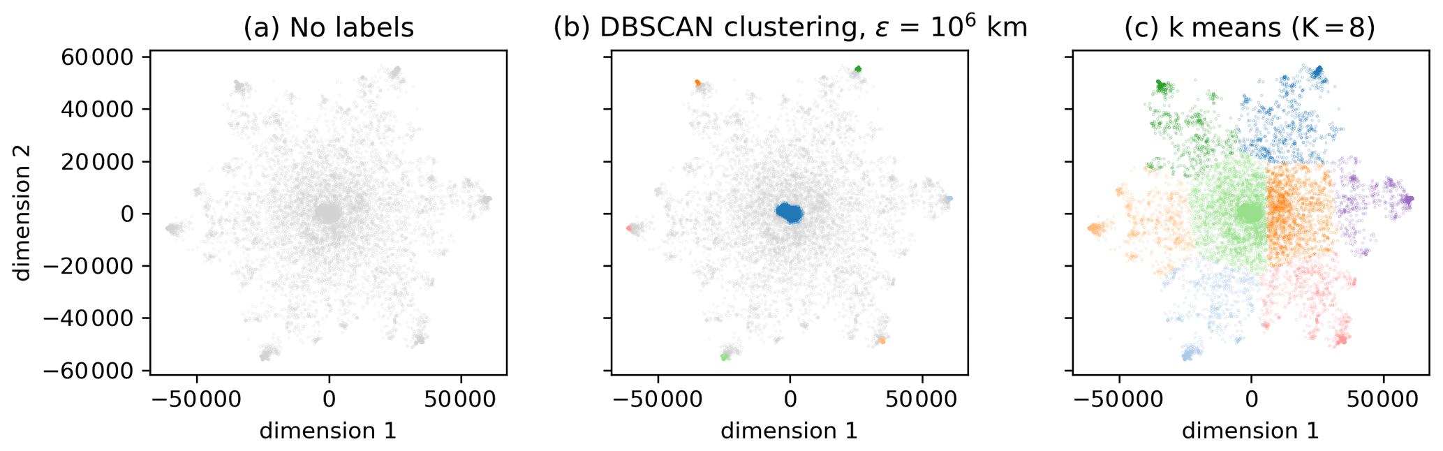
Figure 3(a) A 2D embedding of the classical MDS method (see Sect. 3.2.2) of the trajectories. (b) Labels according to the DBSCAN result of Fig. 4. The six vortices and the jet are clearly visible as dense regions. Grey particles correspond to noise. (c) The k-means clustering result for K=8; see Fig. 5 for the spatial clustering result of k-means.
The corresponding clustering results in real space are shown in Figs. 4 and 5 for OPTICS and k-means, respectively. The jet and the six vortices are clearly recognizable as dense accumulations of points in the 2D space of Fig. 3b (see Fig. 4 for the corresponding colours). The clustering result with k-means in Fig. 5 shows that the clusters corresponding to the vortices are much less focused. In addition, each of the eight clusters in Fig. 3c contains some of the noisy points of Fig. 3b, which shows that using one additional cluster for noise does not work in this situation. It is interesting to note that capturing the noisy data points of Fig. 3b with an additional cluster in k-means is geometrically impossible, simply because k-means clusters are circular. Covering all noisy points without including the centre, i.e. the jet in Fig. 3b, is not possible for k-means.
It should be noted here that the poor performance of k-means in Figs. 3c and 5 is not representative for other methods that use k-means. For example, the method of Banisch and Koltai (2017) captures the coherent structures in the Bickley jet rather well, including the jet in the middle. We emphasize again that we use classical MDS here mostly for visualization purposes as the computation of the classical MDS embedding is difficult for large particle sets. In our case, a dense 12 000×12 000 symmetric matrix has to be diagonalized, which already takes a significant amount of computation time.
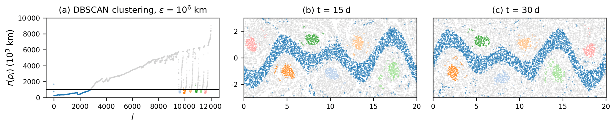
Figure 4Result of DBSCAN clustering of the 2D embedding of the classical MDS method. (a) Reachability plot, with the black line representing the DBSCAN parameter ϵ. (b–c) Corresponding clustering results at different times. Grey particles represent noise. Axis units are in 1000 km.
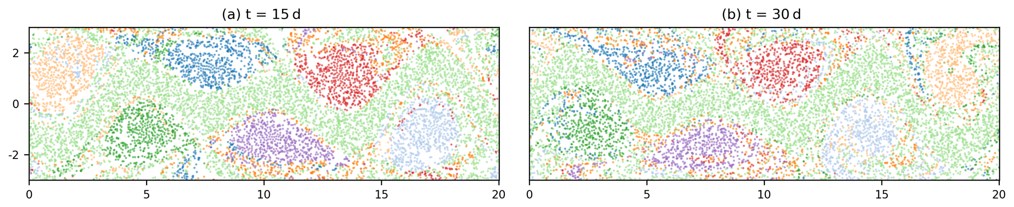
Figure 5Result of K=8 k-means clustering of the 2D embedding from classical MDS (see Fig. 4). Axis units are in 1000 km.
We finally also tested the performance of our algorithm with a random subset of 2000 particles, using data for every 5 d instead of every day (see Fig. A2 in the Appendix). OPTICS still detects the six vortices and the jet, although the cluster boundaries are less clearly defined compared to Fig. 2. Froyland and Junge (2018) detect the vortices and the jet by using the data of 3000 particles only at initial and final times (t=0 and t=40 d). Our method is not able to detect the expected finite-time coherent sets by using only initial and final particle data. This is likely to be a result of the ad hoc direct embedding; see Eq. (3) and the discussion at the end of Sect. 3.4.
4.2 Agulhas rings
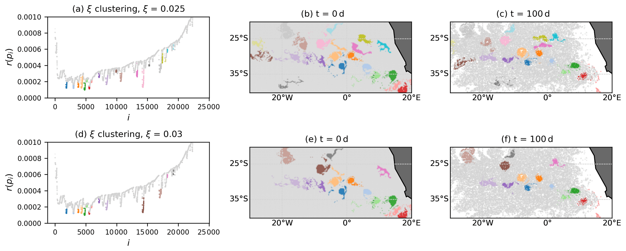
We next apply OPTICS to the Agulhas trajectories. As described in Sect. 2, we have with N=23 821. We choose in the following, which corresponds initially to a square cell of , i.e. a reasonable minimum size of an Agulhas ring. Figure 6 shows the result of the direct embedding. The reachability plot in Fig. 6a is much more jagged than for the Bickley jet model flow (see Fig. 2a). The narrow, deep valleys and the wider valleys in the reachability plot indicate the presence of large- and small-scale coherence patterns. Figure 6a–c show the DBSCAN clustering result for a relatively large value of ϵ. The main separation of fluid domains is between the red and the blue particles, with a few vortices at their boundary. These two water masses are the northern and southern parts of the subtropical gyre in the South Atlantic, with the red particles moving to the west and the blue particles moving to the east. The second and third rows of Fig. 6 show other clustering results for the DBSCAN- and the ξ-clustering method, respectively. The valleys in Fig. 6g with steepest boundaries, as detected by the ξ-clustering method, mostly correspond to eddy-like structures separated by background noise. Note that not all clusters in the figure correspond to eddies. For example, the blue cluster in Fig. 6g–i stays approximately coherent over the considered time interval, although it is certainly not an Agulhas ring. An animation of the detected finite-time coherent sets for the full 2 years of trajectory data, based on the ξ-clustering method as in the last row of Fig. 6, can be found on Zenodo (Wichmann, 2020a), showing that many of the sets stay coherent for significantly longer times than the first 100 d.

Figure 6Result of the OPTICS algorithm applied to the direct embedding of the trajectories with different clustering methods. Grey particles correspond to noise.
Figure 6 shows that, for this situation, the ξ-clustering method detects more Agulhas rings than DBSCAN. While the clustering results shown in the figure all depend on the parameter values for ξ and ϵ, it is visible in the reachability plot of Fig. 6g that the definition of some eddies includes the entire boundary of the valleys, i.e. up to very high reachability values. At the same time, the detection of the large-scale clusters, as in Fig. 6a–c, is not possible with the ξ-clustering method. These findings are in fact expected; see the discussion of the two clustering methods at the end of Sect. 3.3. DBSCAN is best for detecting global density structures, i.e. when the reachability values of all points are compared to the same cut-off ϵ. Regions that are dense locally but not necessarily globally are better detected with the ξ-clustering method. Despite these differences between the two clustering methods, we again emphasize that the main result of OPTICS is the reachability plot itself. Figure 7 shows a colour map at the initial time of the reachability values. We clearly see Agulhas rings as the dark regions corresponding to lowest values of reachability. The regions of large reachability correspond to trajectories that are relatively noisy compared to all the other trajectories.
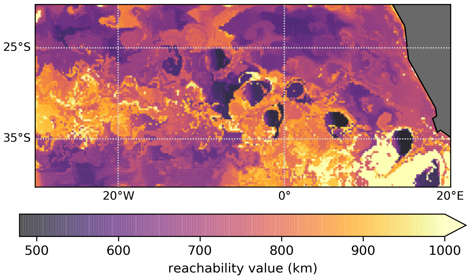
Figure 7Reachability values at the initial time that resulted from the OPTICS algorithm being applied to the direct embedding of the trajectories. The regions with lowest values clearly correspond to Agulhas rings. The colour bar is cut off at a reachability of 1000 km to show the relevant structure of the variations.
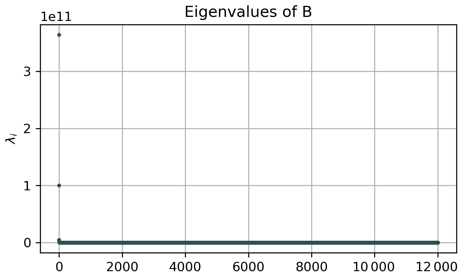
In order to illustrate again the difference between OPTICS and k-means for this example, we choose 12 000 random trajectories and again embed the trajectories in a 2D space with classical MDS (see Sect. 3.2.2). The reduction in the particle set is necessary for simplifying the eigendecomposition of the matrix B in Eq. (4), and we therefore choose . The corresponding spectrum of B is shown in Fig. B1 in the Appendix, showing that there are again two dominant eigenvectors, i.e. visualizing the network in the plane captures the main variance of the data. Figure 8 shows the embedded trajectories together with OPTICS and DBSCAN clustering (Fig. 8b) and k-means (Fig. 8c) for K=40. Figures 9 and 10 show the corresponding clustering results in the fluid domain. It is clear that k-means does not detect a single vortex but instead splits the fluid domain into regions of approximately similar size. OPTICS detects multiple Agulhas rings by finding the deepest valleys in the reachability plot.
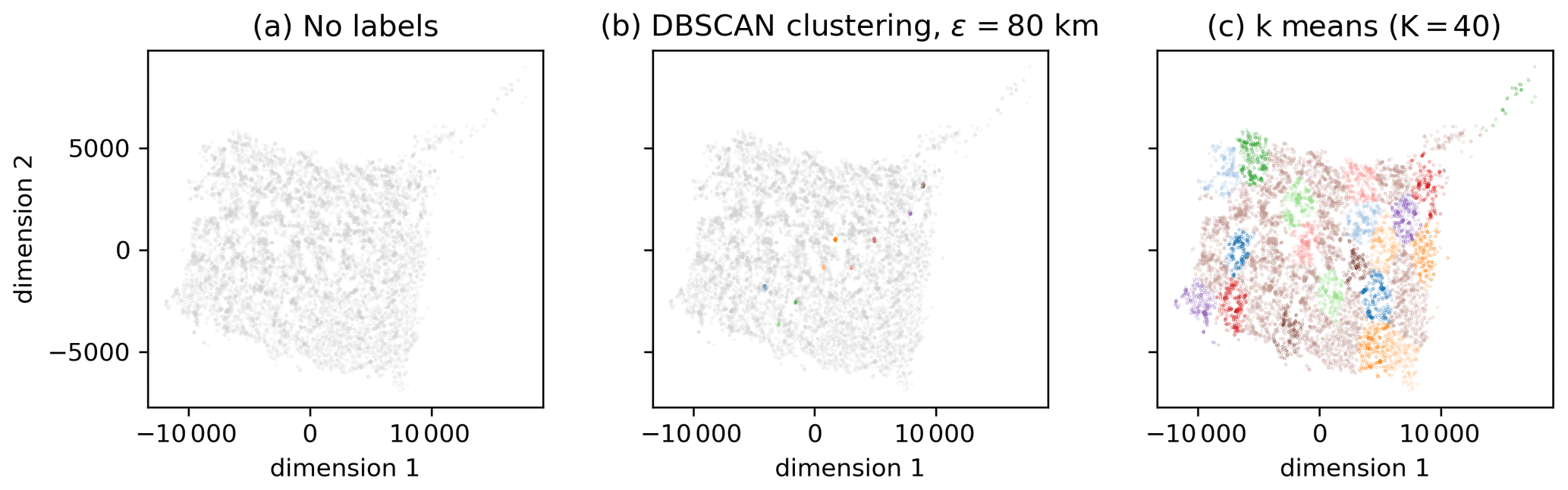
Figure 8Embedding of the Agulhas trajectories in the 2D space defined by the leading eigenvectors of the MDS kernel matrix B. (a) No labels. (b) Clustering labels of OPTICS and DBSCAN (see Fig. 9 for the corresponding plot in the Agulhas region). Grey particles represent noise. (c) The k-means with K=40 (see Fig. 10 for the corresponding plot in the Agulhas domain.)
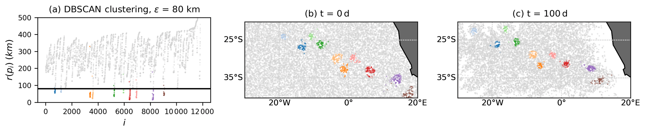
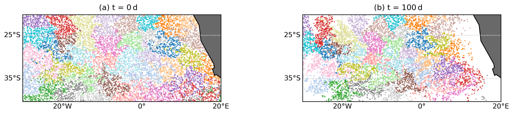
Figure 10Result of the k-means clustering, with K=40 applied to the 2D embedding with classical MDS (see Fig. 8c).
It is interesting to note that the use of classical MDS in Fig. 9 has led to the detection of many of the vortices of Fig. 6d–f with DBSCAN instead of the ξ-clustering method. The transformation to the reduced 2D space has hence led to a simplification of the reachability plot, which now represents the major variations in the distances of the embedded trajectories. At the same time, the large-scale structure of Fig. 6a is not visible any more in Fig. 9. This indicates that exploring more dimensionality-reduction techniques could be useful for future research, in particular for those that are computationally more efficient than classical MDS.
Spectral embeddings derived from networks, together with partition-based clustering, have a similar problem to the one illustrated in Figs. 8c and 10 (Froyland et al., 2019). Similar to the case discussed here, OPTICS can be used to overcome the problems of k-means. We show this in Appendix C for the network proposed by Padberg-Gehle and Schneide (2017) for the Agulhas region, together with a brief introduction to the network and how to construct spectral embeddings. In summary, k-means again fail to detect any of the vortices, while OPTICS detects many of the coherent vortices in the spectrally embedded network. Yet, other flow features are also present that result from the physical motivation of the network definition (see the results in Appendix C).
The abstract embedding of particle trajectories in a metric space with subsequent clustering is a promising field of research for the detection of finite-time coherent sets in oceanography. Yet, most of the existing methods have been based on graph partitioning, which has no concept of noisy, unclustered trajectories. This is a problem for applications in the ocean, where many eddies are transported in a noisy background flow on large domains. This study is motivated by the success of Froyland et al. (2019) in overcoming the problem of graph partitioning by a sophisticated form of trajectory embedding. Here, we show how the density-based clustering algorithm of OPTICS (Ankerst et al., 1999) can be used instead of graph partitioning in order to detect small-scale eddies in large ocean domains. Different from partition-based clustering methods such as k-means, OPTICS does not require one to fix the number of clusters beforehand. Clusters are detected by identifying dense accumulations of points, i.e. groups of trajectories that are close to each other in the embedding space. Coherent groups of particle trajectories can be identified as valleys in the reachability plot computed by the OPTICS algorithm. This plot also has a natural interpretation in terms of cluster hierarchies, i.e. finite-time coherent sets that are by themselves part of a larger-scale finite-time coherent set. Such hierarchies are present in the surface ocean flow, where the subtropical basins are approximately coherent and, at the same time, contain other finite-time coherent structures such as eddies and jets.
We apply OPTICS to Lagrangian particle trajectories directly, in the spirit of Froyland and Padberg-Gehle (2015). OPTICS successfully detects the expected coherent structures in the Bickley jet model flow, separating the six vortices and the jet from background noise. We also apply OPTICS to simulated trajectories in the eastern South Atlantic and successfully identify Agulhas rings separated by noise. We visualize the difference between OPTICS and k-means with a 2D embedding of the trajectories, based on classical multidimensional scaling. We also show how OPTICS can be applied to the spectral embedding of the particle-based network proposed by Padberg-Gehle and Schneide (2017), providing a necessary amendment to their method of detecting coherent vortices in a large ocean domain, i.e. when k-means fails. Our method is very simple to implement in Python, as OPTICS is available in the scikit-learn library in Python. While we here present the results of OPTICS with three different kinds of embeddings, it is likely that OPTICS also works for other trajectory embeddings, such as the spectral embeddings of Banisch and Koltai (2017) or Froyland and Junge (2018). Using such dynamically motivated embeddings instead of the ad hoc direct embedding presented here could be a promising direction for future research.
Extending our method to data sets with more trajectories can be made more efficient by choosing a finite generating distance for OPTICS (Ankerst et al., 1999). While this is better from a computational point of view, it requires some knowledge or intuition about the spatial distribution of the embedded trajectories. A major challenge for the method proposed here is the embedding dimension. For long trajectories, it is necessary to reduce the dimensionality of the trajectories before applying OPTICS. A complication here is the desired property of an embedding to preserve both local and global distances in order to make full use of the hierarchical properties of OPTICS. This means, for example, that the popular method of a locally linear embedding (Roweis and Saul, 2000) is not suitable, unless only the small-scale (densest) finite-time coherent sets are to be detected. Using classical multidimensional scaling (MDS), as we did here to visualize the clustering results, preserves local and global distances in principle, although our results indicate that the large-scale coherence structure in the Agulhas flow is less pronounced for the classical MDS embedding compared to the full embedding of trajectories. In any case, classical MDS is not an option for very large data sets, as it requires the diagonalization of a dense symmetric square matrix of size equal to the particle number. Spectral embeddings of derived networks, such as the ones of Hadjighasem et al. (2016), Padberg-Gehle and Schneide (2017) and Banisch and Koltai (2017), are useful for achieving lower dimensional embeddings, but they come with the introduction of additional parameters for the network construction and heuristics to truncate the embedding dimension. Further research into other nonlinear dimensionality-reduction techniques that have not been explored in the context of finite-time coherent sets can lead to more efficient and robust methods.
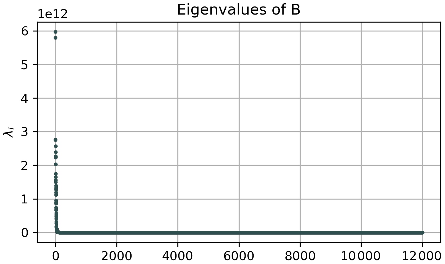
Figure A1Spectrum of the classical MDS kernel matrix B for the Bickley jet flow. It is evident that there are two dominant eigenvalues. We choose the vectors corresponding to these first two eigenvalues as embedding vectors in Sect. 4.1.
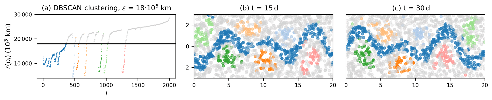
Figure A2Result of the OPTICS algorithm for a random subset of 2000 particles in the Bickley jet flow, with particle data every 5 d instead of every day. To account for the smaller number of particles, we set for this case. The six vortices and the jet are still clearly visible.
To demonstrate that OPTICS can also be applied to the spectral embedding of a particle-based network, we use the network proposed by Padberg-Gehle and Schneide (2017). If we have a set of particle trajectories xi(t), where , and with N the number of particles and T is the number of time steps, the network is defined as follows:
Here, denotes the Euclidean norm, and d>0 is a fixed predetermined cut-off parameter. See Padberg-Gehle and Schneide (2017) for a discussion on the choice of d (called ϵ in Padberg-Gehle and Schneide, 2017). Similar to Padberg-Gehle and Schneide (2017), we embed the nodes in a lower dimensional space ℝK by means of the eigenvectors of its random walk Laplacian (see, e.g., Von Luxburg, 2007) as follows:
where D is a diagonal matrix with . The embedding of node i is defined by the following:
where are the right eigenvectors corresponding to the largest eigenvalues λi of Lr. The eigenvalues are assumed to be ordered in descending order, i.e. . The classical simultaneous K-way normalized cut proceeds with applying the k-means algorithm to the embedding defined in Eq. (C3) to detect K clusters (Von Luxburg, 2007), resulting in an approximate solution to the normalized cut problem (Shi and Malik, 2000).
Figure C1 shows the spectrum of the resulting random walk Laplacian with d=200 km. No obvious spectral gap is visible that would suggest a truncation of the embedding space. Figure C2 shows the clustering result if we apply a k-means algorithm, as suggested by Padberg-Gehle and Schneide (2017), to detect K=40 clusters. It is visible that the partition-based k-means clustering method does not detect any individual Agulhas rings but instead partitions the state space into regions of approximately equal size.
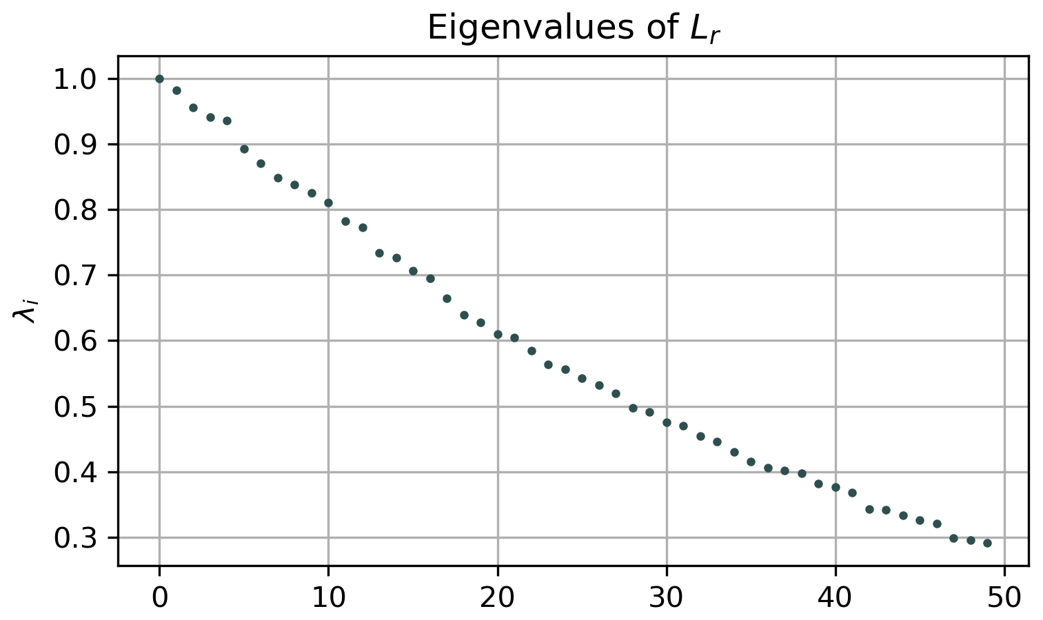
Figure C1Spectrum of the random walk Laplacian (see Eq. C2) of the network proposed by Padberg-Gehle and Schneide (2017) applied to the Agulhas trajectory data. No clear gap exists to suggest a truncation of the embedding.
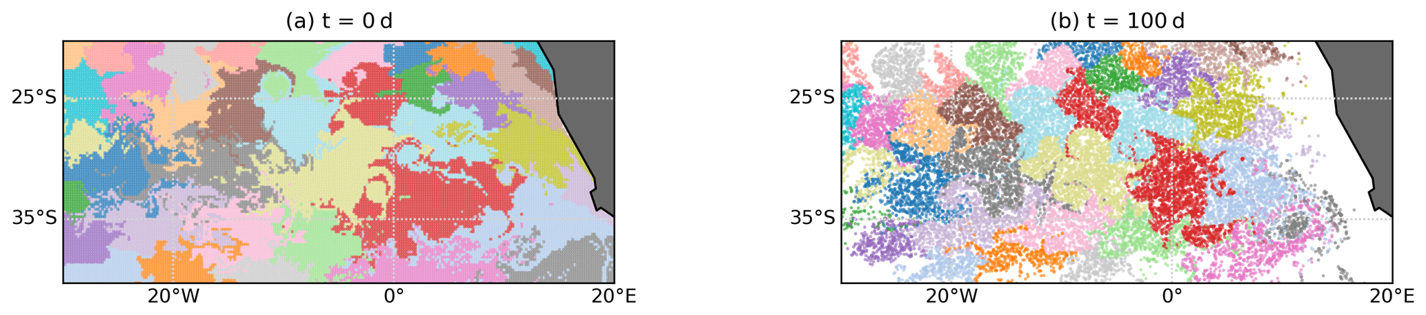
Figure C2Result of k-means clustering applied to the 40 leading eigenvectors of the random walk Laplacian (see Eq. C2), looking for 40 clusters. No individual vortices are detected.
Applying OPTICS instead of k-means with a subsequent ξ clustering detects some of the Agulhas rings (see Fig. C3), where we choose as in Sect. 4.2. Note also that structures other than typical circular eddies are detected. While this depends on the clustering parameter ξ (or ϵ for DBSCAN), this is also a consequence of the physically motivated network defined by Eq. (C3), where particles are connected equally if they are close to each other at least once at a point in time. This is different from the direct embedding, where we require particles to stay close to each other along the entire trajectory.
All code is available at https://doi.org/10.5281/zenodo.4426287 (Wichmann, 2021a), including the code to generate the Bickley jet trajectories. The data for the virtual particles in the South Atlantic are available at https://doi.org/10.5281/zenodo.3899942 (Wichmann, 2020b). Details on the Parcels simulation for the virtual trajectories in the ocean can be found at the GitHub repository of our previous paper, i.e. https://doi.org/10.5281/zenodo.4426310 (Wichmann, 2021b). The NEMO N006 data are kindly provided by Andrew Coward at NOC Southampton, UK, and can be downloaded at http://opendap4gws.jasmin.ac.uk/thredds/nemo/root/catalog.html (last access: 10 March 2019).
DW performed the analysis, with support from CK, EvS and HAD. DW wrote the paper, and all authors jointly edited and revised it.
The authors declare that they have no conflict of interest.
David Wichmann, Christian Kehl and Erik van Sebille have been supported through funding from the European Research Council (ERC) under the European Union Horizon 2020 research and innovation programme (grant no. 715386). This work was partially carried out on the Dutch national e-infrastructure, with the support of SURF Cooperative (project no. 16371). We thank Andrew Coward for providing the ORCA-N006 simulation data.
This research has been supported by the European Research Council (TOPIOS (grant no. 715386)).
This paper was edited by Juan Restrepo and reviewed by two anonymous referees.
Ankerst, M., Breunig, M. M., Kriegel, H.-P., and Sander, J.: OPTICS: Ordering Points to Identify the Clustering Structure, ACM Sigmod Record, 28, 49–60, https://doi.org/10.1145/304181.304187, 1999. a, b, c, d, e, f, g, h, i, j, k, l
Banisch, R. and Koltai, P.: Understanding the geometry of transport: Diffusion maps for Lagrangian trajectory data unravel coherent sets, Chaos: An Interdisciplinary J. Nonlinear Sci., 27, 035804, https://doi.org/10.1063/1.4971788, 2017. a, b, c, d, e, f, g, h, i, j, k, l, m, n, o
Beron-Vera, F. J., Wang, Y., Olascoaga, M. J., Goni, G. J., and Haller, G.: Objective Detection of Oceanic Eddies and the Agulhas Leakage, J. Phys. Oceanogr., 43, 1426–1438, https://doi.org/10.1175/JPO-D-12-0171.1, 2013. a, b
Bickley, W.: LXXIII. The plane jet, The London, Edinburgh, and Dublin Philosophical Magazine and Journal of Science, 23, 727–731, https://doi.org/10.1080/14786443708561847, 1937. a
Brach, L., Deixonne, P., Bernard, M. F., Durand, E., Desjean, M. C., Perez, E., van Sebille, E., and ter Halle, A.: Anticyclonic eddies increase accumulation of microplastic in the North Atlantic subtropical gyre, Marine Pollution Bulletin, 126, 191–196, https://doi.org/10.1016/j.marpolbul.2017.10.077, 2018. a
del Castillo-Negrete, D. and Morrison, P.: Chaotic transport by Rossby waves in shear flow, Phys. Fluids A, 5, 948–965, https://doi.org/10.1063/1.858639, 1993. a
Delandmeter, P. and van Sebille, E.: The Parcels v2.0 Lagrangian framework: new field interpolation schemes, Geosci. Model Dev., 12, 3571–3584, https://doi.org/10.5194/gmd-12-3571-2019, 2019. a
Dencausse, G., Arhan, M., and Speich, S.: Routes of Agulhas rings in the southeastern Cape Basin, Deep-Sea Res. Pt. I, 57, 1406–1421, https://doi.org/10.1016/j.dsr.2010.07.008, 2010. a
Dong, C., McWilliams, J. C., Liu, Y., and Chen, D.: Global heat and salt transports by eddy movement, Nature Commun., 5, 3294, https://doi.org/10.1038/ncomms4294, 2014. a
Dussin, R., Barnier, B., and Brodeau, L.: The making of Drakkar forcing set DFS5, Tech. rep., LGGE, Grenoble, France, 2016. a
Ester, M., Kriegel, H.-P., Sander, J., and Xu, X.: A Density-Based Algorithm for Discovering Clusters in Large Spatial Databases with Noise, in: Proceedings of the Second International Conference on Knowledge Discovery and Data Mining, KDD'96, 226–231, AAAI Press, 1996. a, b, c
Fouss, F., Saerens, M., and Shimbo, M.: Algorithms and models for network data and link analysis, Cambridge University Press, Cambridge, https://doi.org/10.1017/CBO9781316418321, 2016. a, b
Froyland, G. and Junge, O.: Robust FEM-based extraction of finite-time coherent sets using scattered, sparse, and incomplete trajectories, SIAM Journal on Applied Dynamical Systems, 17, 1891–1924, https://doi.org/10.1137/17M1129738, 2018. a, b, c, d, e, f, g, h, i, j, k, l, m, n
Froyland, G. and Padberg-Gehle, K.: A rough-and-ready cluster-based approach for extracting finite-time coherent sets from sparse and incomplete trajectory data, Chaos: An Interdisciplinary J. Nonlinear Sci., 25, 087406, https://doi.org/10.1063/1.4926372, 2015. a, b, c, d, e, f, g, h, i, j, k
Froyland, G., Santitissadeekorn, N., and Monahan, A.: Transport in time-dependent dynamical systems: Finite-time coherent sets, Chaos: An Interdisciplinary J. Nonlinear Sci., 20, 043116, https://doi.org/10.1063/1.3502450, 2010. a, b
Froyland, G., Stuart, R. M., and van Sebille, E.: How well-connected is the surface of the global ocean?, Chaos: An Interdisciplinary J. Nonlinear Sci., 24, 033126, https://doi.org/10.1063/1.4892530, 2014. a
Froyland, G., Horenkamp, C., Rossi, V., and van Sebille, E.: Studying an Agulhas ring's long-term pathway and decay with finite-time coherent sets, Chaos: An Interdisciplinary J. Nonlinear Sci., 25, 083119, https://doi.org/10.1063/1.4927830, 2015. a
Froyland, G., Rock, C. P., and Sakellariou, K.: Sparse eigenbasis approximation: Multiple feature extraction across spatiotemporal scales with application to coherent set identification, Communications in Nonlinear Science and Numerical Simulation, 77, 81–107, https://doi.org/10.1016/j.cnsns.2019.04.012, 2019. a, b, c, d, e, f, g, h, i, j, k, l, m, n, o, p, q
Hadjighasem, A., Karrasch, D., Teramoto, H., and Haller, G.: Spectral-clustering approach to Lagrangian vortex detection, Phys. Rev. E, 93, 063107, https://doi.org/10.1103/PhysRevE.93.063107, 2016. a, b, c, d, e, f, g, h, i, j, k, l, m
Hadjighasem, A., Farazmand, M., Blazevski, D., Froyland, G., and Haller, G.: A critical comparison of Lagrangian methods for coherent structure detection, Chaos: An Interdisciplinary J. Nonlinear Sci., 27, 053104, https://doi.org/10.1063/1.4982720, 2017. a, b, c, d
Haller, G. and Beron-Vera, F. J.: Coherent Lagrangian vortices: The black holes of turbulence, J. Fluid Mech., 731, https://doi.org/10.1017/jfm.2013.391, 2013. a
Lange, M. and van Sebille, E.: Parcels v0.9: prototyping a Lagrangian ocean analysis framework for the petascale age, Geosci. Model Dev., 10, 4175–4186, https://doi.org/10.5194/gmd-10-4175-2017, 2017. a
Ma, T. and Bollt, E. M.: Relatively Coherent Sets as a Hierarchical Partition Method, Int. J. Bifurcat.Chaos, 23, 1330026, https://doi.org/10.1142/S0218127413300267, 2013. a, b
Madec, G.: NEMO ocean engine, Note du Pôle de modélisation, No 27, 2008. a
Padberg-Gehle, K. and Schneide, C.: Network-based study of Lagrangian transport and mixing, Nonlin. Processes Geophys., 24, 661–671, https://doi.org/10.5194/npg-24-661-2017, 2017. a, b, c, d, e, f, g, h, i, j, k, l, m, n, o, p, q, r, s, t
Roweis, S. T. and Saul, L. K.: Nonlinear Dimensionality Reduction by Locally Linear Embedding, Science, 290, 2323–2326, https://doi.org/10.1126/science.290.5500.2323, 2000. a
Schneide, C., Pandey, A., Padberg-Gehle, K., and Schumacher, J.: Probing turbulent superstructures in Rayleigh-Bénard convection by Lagrangian trajectory clusters, Phys. Rev. Fluids, 3, 113501, https://doi.org/10.1103/PhysRevFluids.3.113501, 2018. a, b, c, d, e
Schouten, M. W., de Ruijter, W. P. M., van Leeuwen, P. J., and Lutjeharms, J. R. E.: Translation, decay and splitting of Agulhas rings in the southeastern Atlantic Ocean, J. Geophys. Res.-Oceans, 105, 21913–21925, https://doi.org/10.1029/1999jc000046, 2000. a
Shi, J. and Malik, J.: Normalized cuts and image segmentation, IEEE Transactions on Pattern Analysis and Machine Intelligence, 22, 888–905, https://doi.org/10.1109/34.868688, 2000. a, b
Tarshish, N., Abernathey, R., Zhang, C., Dufour, C. O., Frenger, I., and Griffies, S. M.: Identifying Lagrangian coherent vortices in a mesoscale ocean model, Ocean Model., 130, 15–28, https://doi.org/10.1016/j.ocemod.2018.07.001, 2018. a
van Sebille, E., Aliani, S., Law, K. L., Maximenko, N., Alsina, J. M., Bagaev, A., Bergmann, M., Chapron, B., Chubarenko, I., Cózar, A., Delandmeter, P., Egger, M., Fox-Kemper, B., Garaba, S. P., Goddijn-Murphy, L., Hardesty, B. D., Hoffman, M. J., Isobe, A., Jongedijk, C. E., Kaandorp, M. L., Khatmullina, L., Koelmans, A. A., Kukulka, T., Laufkötter, C., Lebreton, L., Lobelle, D., Maes, C., Martinez-Vicente, V., Morales Maqueda, M. A., Poulain-Zarcos, M., Rodríguez, E., Ryan, P. G., Shanks, A. L., Shim, W. J., Suaria, G., Thiel, M., Van Den Bremer, T. S., and Wichmann, D.: The physical oceanography of the transport of floating marine debris, Environ. Res. Lett., 15, 023003, https://doi.org/10.1088/1748-9326/ab6d7d, 2020. a
Von Luxburg, U.: A Tutorial on spectral clustering, Stat. Comput., 17, 395–416, https://doi.org/10.1007/s11222-007-9033-z, 2007. a, b
Wichmann, D.: Animation of finite-time coherent sets in the Agulhas region, Zenodo, https://doi.org/10.5281/zenodo.4103741, 2020a. a
Wichmann, D.: Lagrangian particle dataset (2 years) for Agulhas region surface flow, Zenodo, https://doi.org/10.5281/zenodo.3899942, 2020b. a, b
Wichmann, D.: OceanParcels/coherent_vortices_OPTICS: Release for publication of corresponding paper (Version v1.0), Zenodo, https://doi.org/10.5281/zenodo.4426287, 2021a. a
Wichmann, D.: OceanParcels/near_surface_microplastic: Release of code for near-surface microplastic simulations, Zenodo, https://doi.org/10.5281/zenodo.4426310, 2021b. a
Wichmann, D., Kehl, C., Dijkstra, H. A., and van Sebille, E.: Detecting flow features in scarce trajectory data using networks derived from symbolic itineraries: an application to surface drifters in the North Atlantic, Nonlin. Processes Geophys., 27, 501–518, https://doi.org/10.5194/npg-27-501-2020, 2020. a
- Abstract
- Introduction
- Trajectory data sets
- Methods
- Results
- Conclusions
- Appendix A: Additional figures for the Bickley jet flow
- Appendix B: Additional figures for the Agulhas flow
- Appendix C: Detecting Agulhas rings with a particle-based network
- Code and data availability
- Author contributions
- Competing interests
- Acknowledgements
- Financial support
- Review statement
- References